Assessment of Landslide-Prone Areas and Their Zonation Using Logistic Regression, LogitBoost, and NaïveBayes Machine-Learning Algorithms


Abstract
:1. Introduction
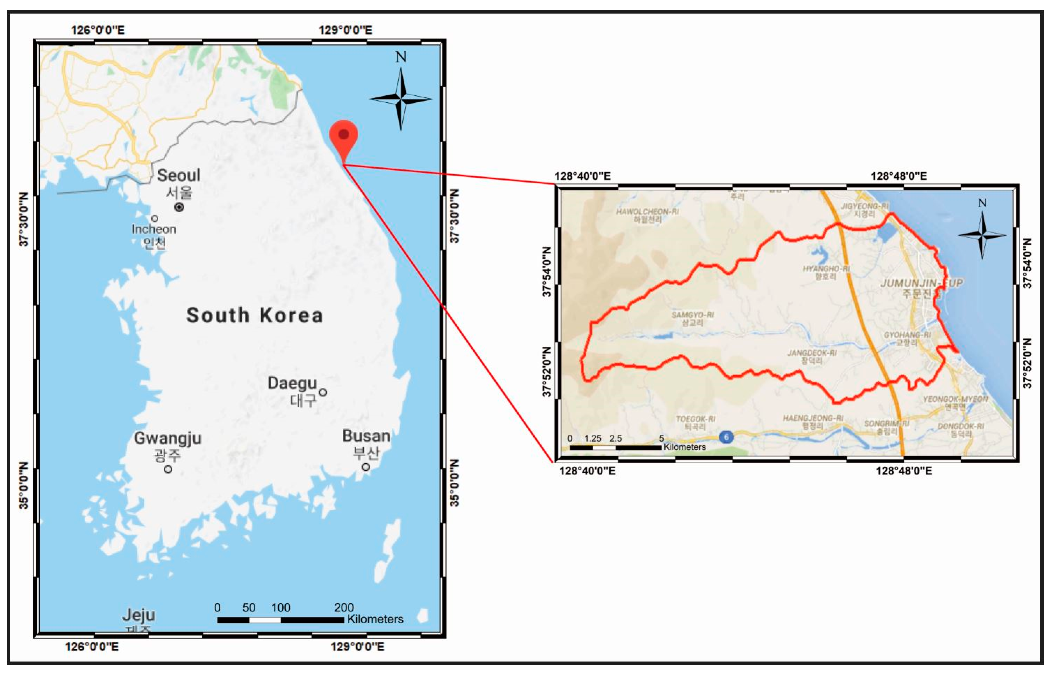
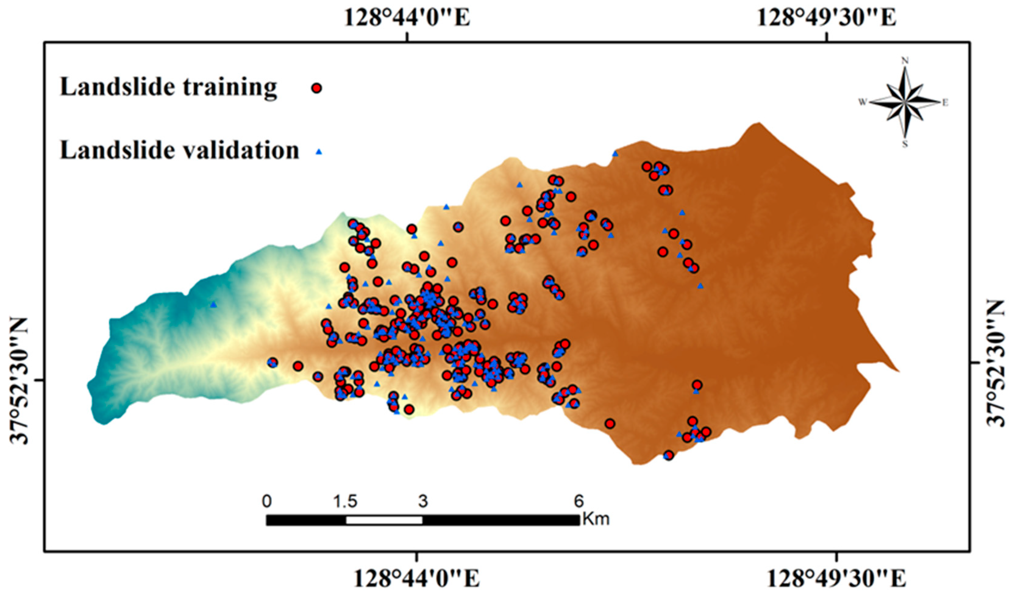
2. Study Area
3. Data Used
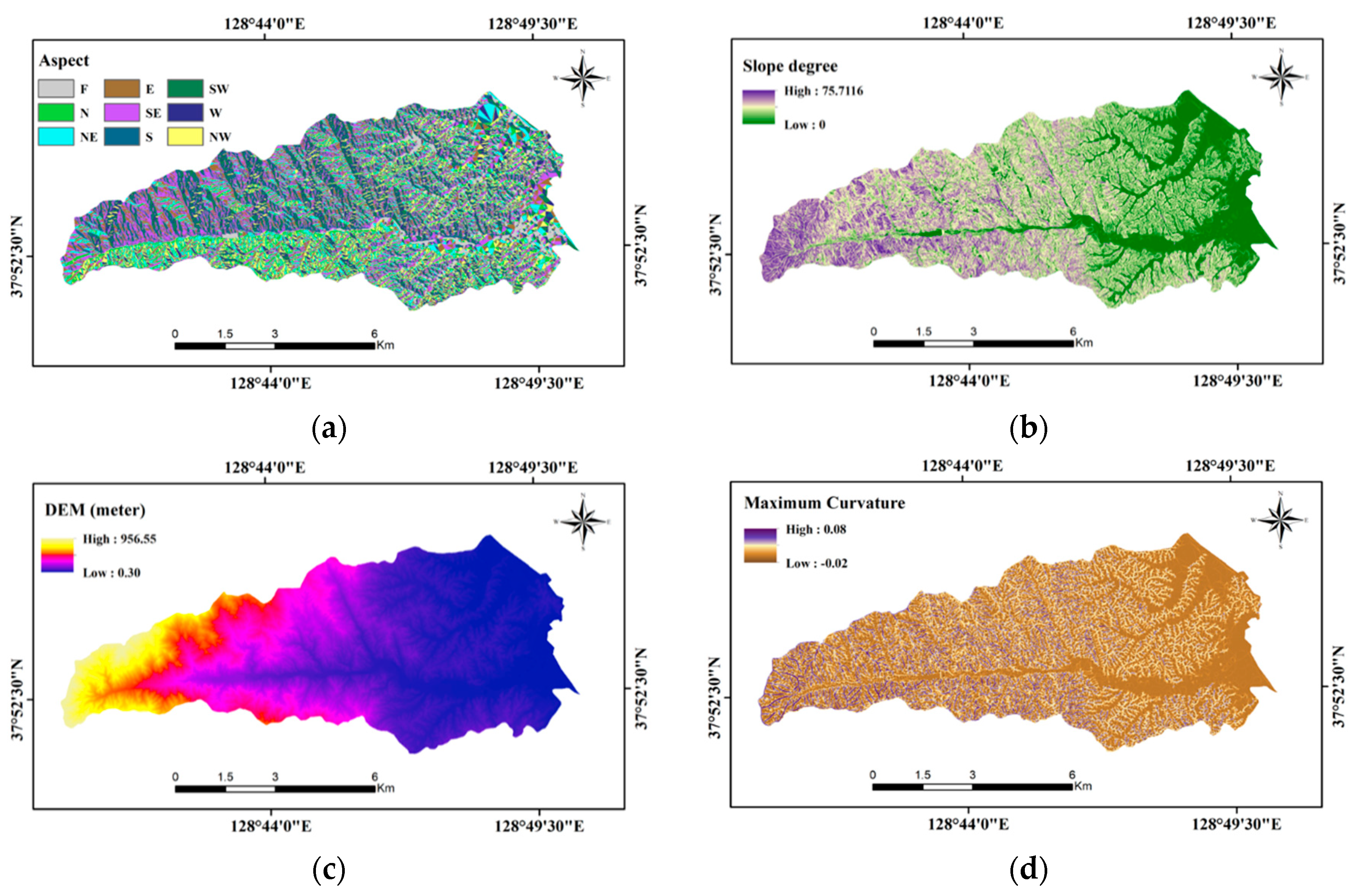
3.1. Aspect
3.2. Slope Gradient
3.3. Altitude
3.4. Curvature (Maximum and Profile)
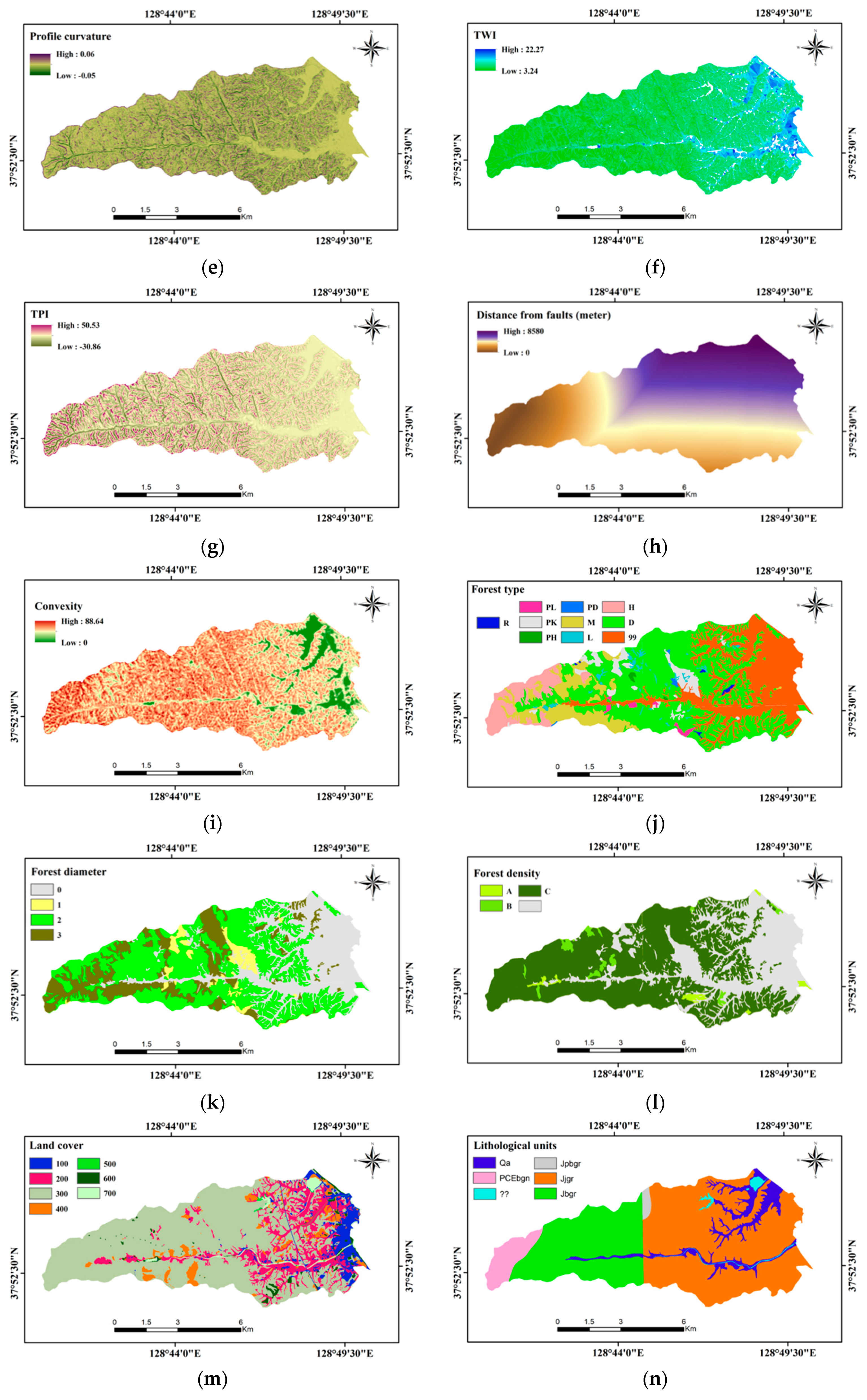
3.5. Topographic Wetness Index (TWI)
3.6. Topographic Positioning Index (TPI)
3.7. Distance from Fault
3.8. Convexity
3.9. Forest Factors (Forest Type, Forest Diameter, and Forest Density)
3.10. Land Use/Land Cover (LULC)
3.11. Lithology
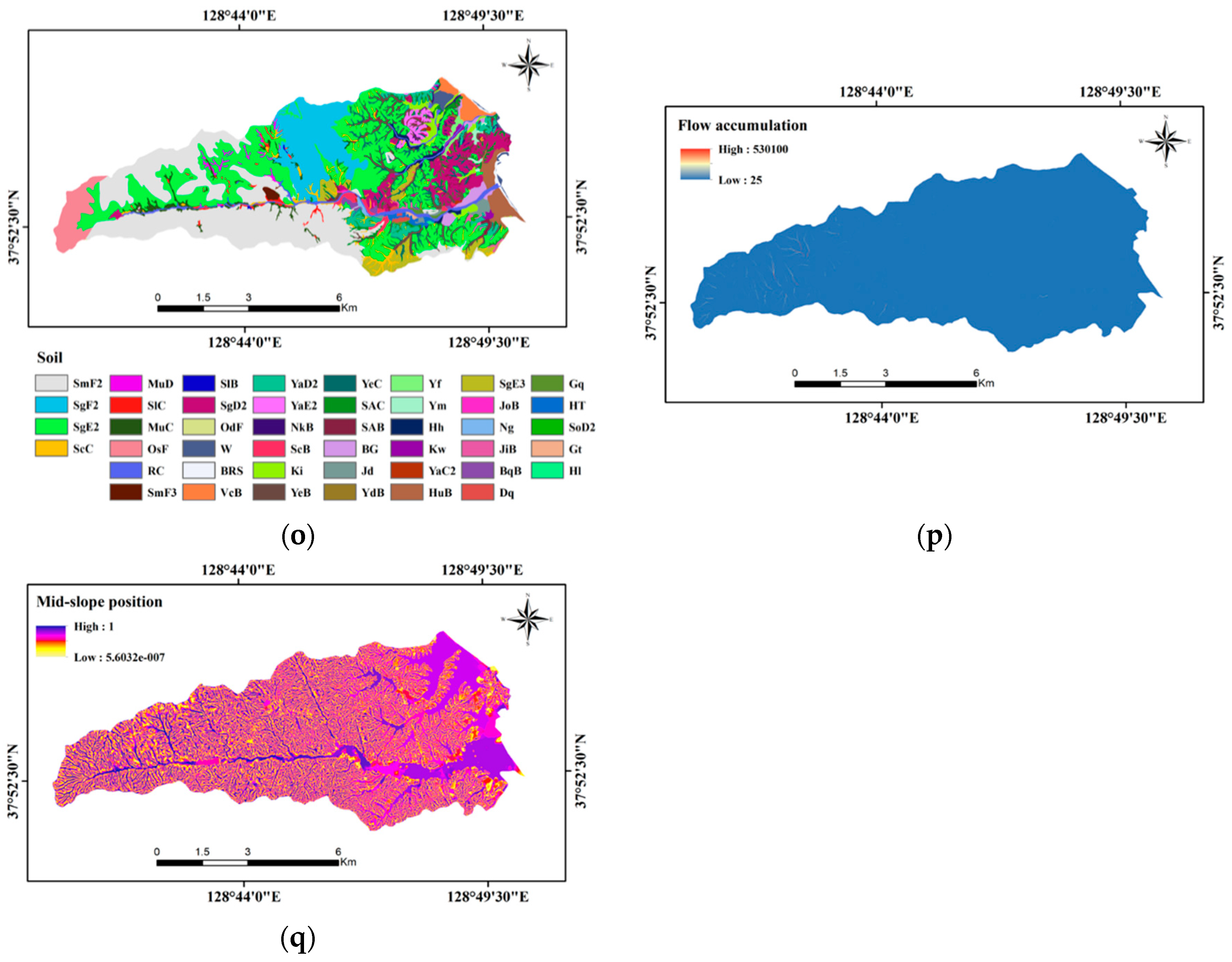
3.12. Soil
3.13. Flow Accumulation
3.14. Mid-Slope Position
4. Multicolinearity of Landslide Effective Factors
5. Modeling for Landslide Susceptibility Zonation
5.1. Logistic Regression (LR)
5.2. LogitBoost (LB)
5.3. NaïveBayes (NB)
5.4. Analysis of Spatial Relationship between Landslide Location and Effective Factors Based on Frequency Ratio (FR)
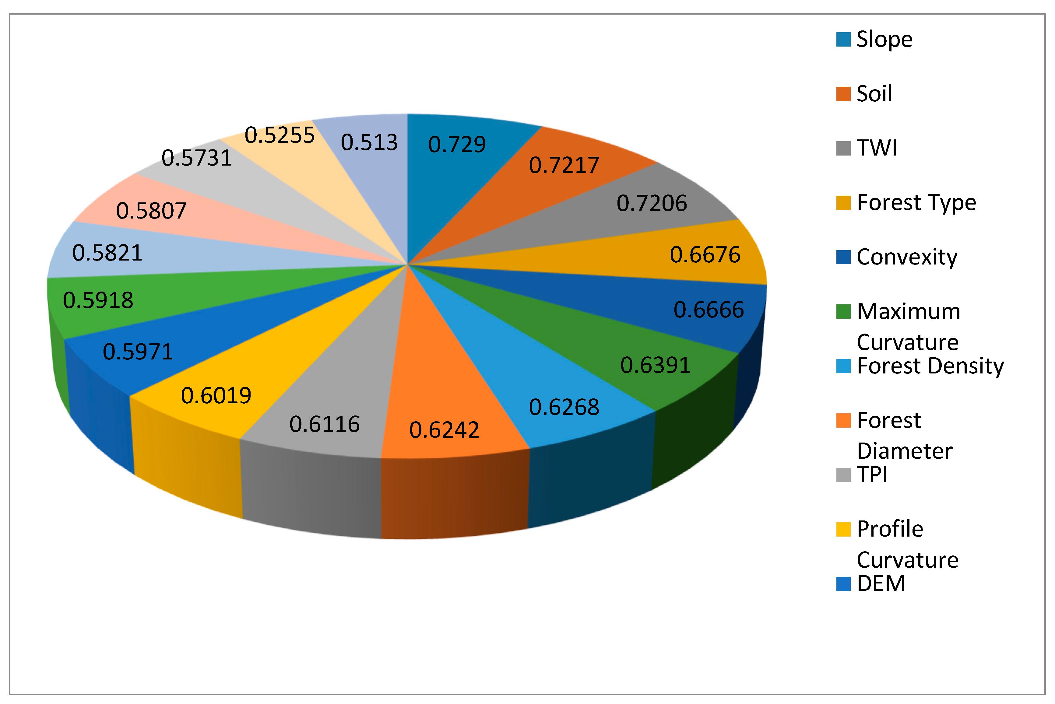
5.5. Analysis of Independent Variable’s Importance
6. Results and Discussion
6.1. Multicollinearity Analysis
6.2. Spatial Relationship between Landslide Locations and Effective Factors
6.3. Variable Contribution Analysis
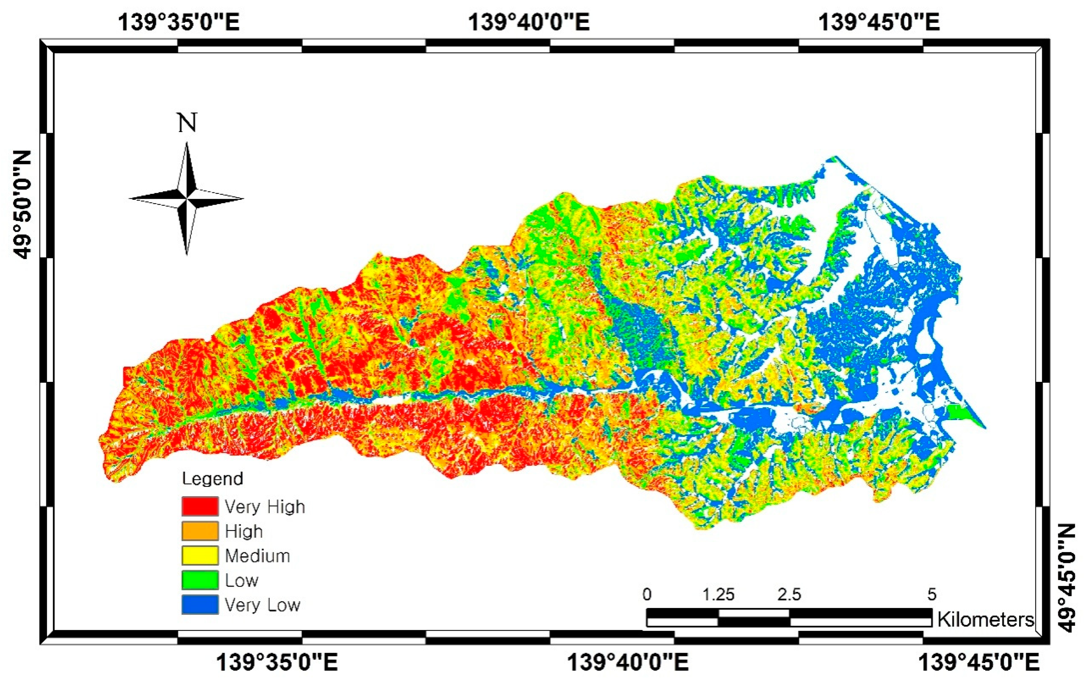
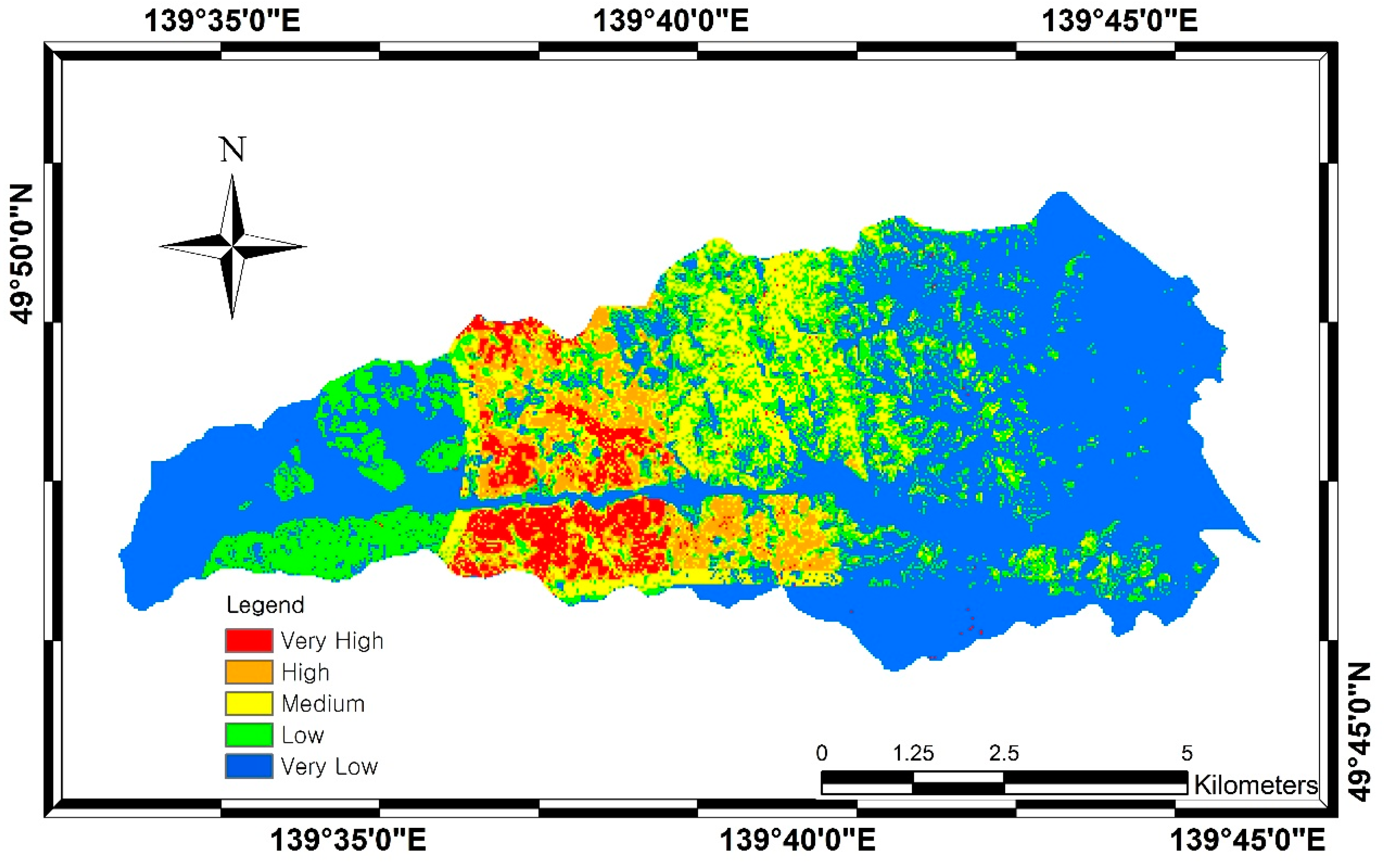
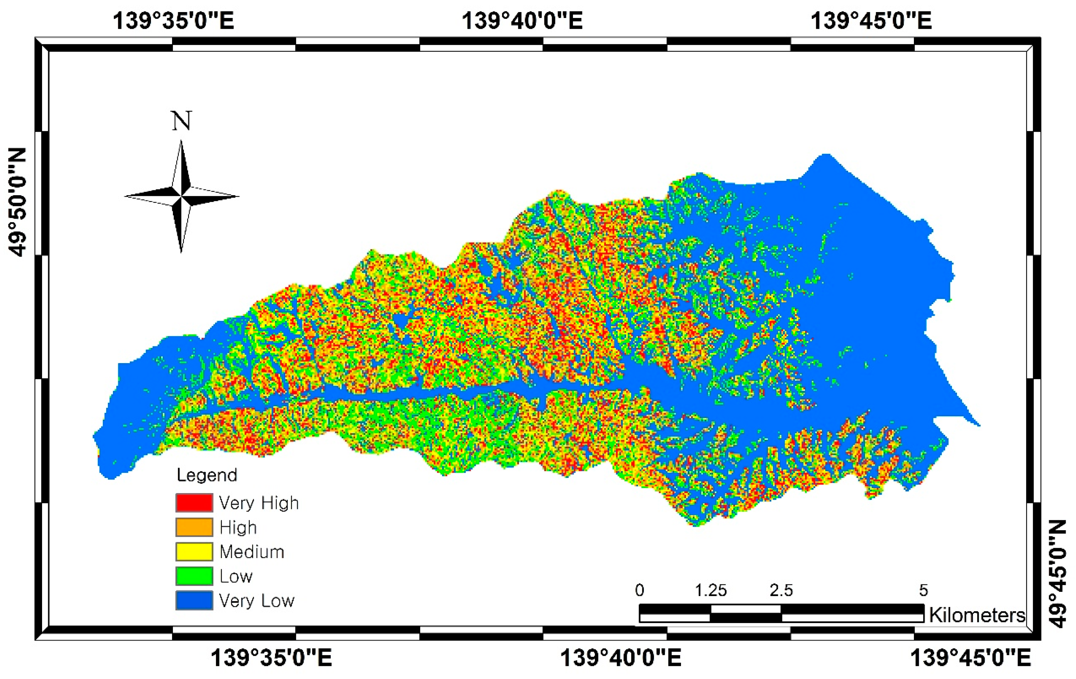
6.4. Landslide Susceptibility Models
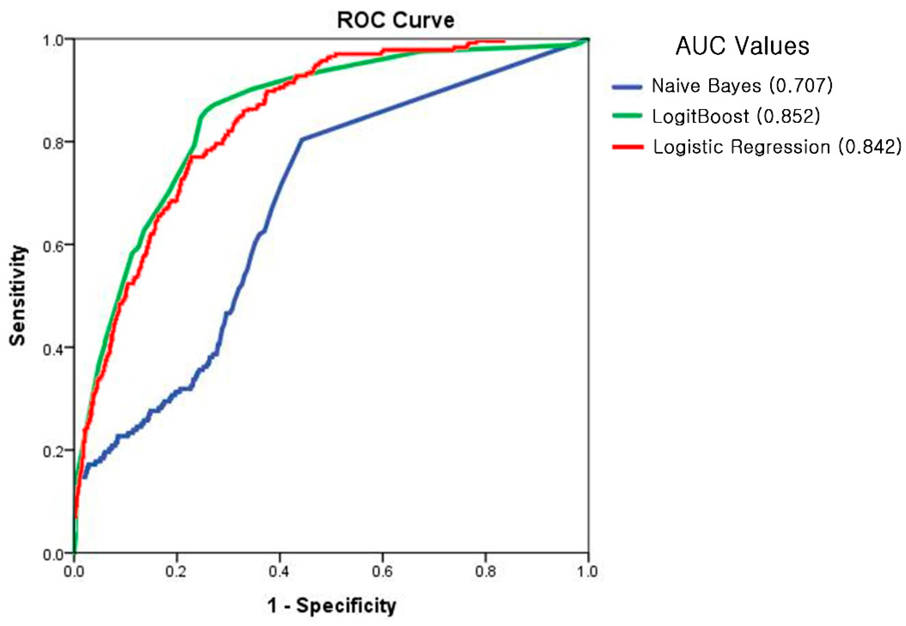
6.5. Accuracy Assessment and Their Comparison
7. Conclusions
Author Contributions
Funding
Acknowledgments
Conflicts of Interest
References
- Lee, S.; Choi, J.; Min, K. Probabilistic landslide hazard mapping using GIS and remote sensing data at Boun, Korea. Int. J. Remote Sens. 2004, 25, 2037–2052. [Google Scholar] [CrossRef]
- Lee, S.; Pradhan, B. Probabilistic Landslide Hazards and Risk Mapping on Penang Island, Malaysia. J. Earth Syst. Sci. 2006, 115, 661–672. [Google Scholar] [CrossRef]
- Varnes, D.J. Slope movement types and processes. In Landslides Analysis and Control; Schuster, R.L., Krizek, R.J., Eds.; Transportation Research Board National Academy of Sciences: Washington, DC, USA, 1978; pp. 11–33. ISBN 0-309-02804-3. [Google Scholar]
- Smith, K. Environmental Hazards: Assessing Risk and Reducing Disaster, 6th ed.; Routledge: Abingdon, UK, 2013; pp. 205–217. ISBN 978-0415681063. [Google Scholar]
- Wang, L.; Sawada, K.; Moriguchi, S. Landslide Susceptibility Mapping by Using Logistic Regression Model with Neighborhood Analysis: A Case Study in Mizunami City. Int. J. GEOMATE 2011, 1, 99–104. [Google Scholar] [CrossRef]
- Pourghasemi, H.R.; Pradhan, B.; Gokceoglu, C.; Moezzi, K.D. Landslide susceptibility mapping using a spatial multi criteria evaluation model at Haraz watershed, Iran. In Terrigenous Mass Movements; Pradhan, B., Buchroithner, M., Eds.; Springer: Berlin/Heidelberg, Germany, 2012; pp. 23–49. ISBN 978-3-642-25495-6. [Google Scholar]
- Basu, T.; Pal, S. Identification of landslide susceptibility zones in Gish River basin, West Bengal, India. Georisk Assess. Manag. Risk Eng. Syst. Geohazards 2018, 12, 14–28. [Google Scholar] [CrossRef]
- Betts, H.; Basher, L.; Dymond, J.; Herzig, A.; Marden, M.; Phillips, C. Development of a landslide component for a sediment budget model. Environ. Model. Softw. 2017, 92, 28–39. [Google Scholar] [CrossRef]
- Pourghasemi, H.R.; Rahmati, O. Prediction of the landslide susceptibility: Which algorithm, which precision? Catena 2018, 162, 177–192. [Google Scholar] [CrossRef]
- Ayalew, L.; Yamagishi, H. The application of GIS-based logistic regression for landslide susceptibility mapping in the Kakuda-Yahiko Mountains, Central Japan. Geomorphology 2005, 65, 15–31. [Google Scholar] [CrossRef]
- Zare, M.; Pourghasemi, H.R.; Vafakhah, M.; Pradhan, B. Landslide susceptibility mapping at Vaz Watershed (Iran) using an artificial neural network model: A comparison between multilayer perceptron (MLP) and radial basic function (RBF) algorithms. Arab. J. Geosci. 2013, 6, 2873–2888. [Google Scholar] [CrossRef] [Green Version]
- Lee, E.M.; Jones, D.K.C. Landslide Risk Assessment; Thomas Telford: London, UK, 2004; p. 454. ISBN 0-7277-3171-8. [Google Scholar]
- Pourghasemi, H.R.; Moradi, H.R.; Aghda, S.F.; Gokceoglu, C.; Pradhan, B. GIS-based landslide susceptibility mapping with probabilistic likelihood ratio and spatial multi-criteria evaluation models (North of Tehran, Iran). Arab. J. Geosci. 2014, 7, 1857–1878. [Google Scholar] [CrossRef]
- Hasekiogullari, G.D.; Ercanoglu, M.A. A new approach to use AHP in landslide susceptibility mapping: A case study at Yenice (Karabuk, NW Turkey). Nat. Hazards 2012, 63, 1157–1179. [Google Scholar] [CrossRef]
- Bijukchhen, S.M.; Kayastha, P.; Dhital, M.R. A Comparative Evaluation of Heuristic and Bivariate Statistical Modeling for Landslide Susceptibility Mappings in Ghurmi-Dhad Khola, East Nepal. Arab. J. Geosci. 2013, 6, 2727–2743. [Google Scholar] [CrossRef]
- Kayastha, P.; Dhital, M.R.; Smedt, F.D. Evaluation and Comparison of GIS Based Landslide Susceptibility Mapping Procedures in Kulekhani Watershed, Nepal. J. Geol. Soc. India 2013, 81, 219–231. [Google Scholar] [CrossRef]
- Pradhan, B.; Lee, S. Landslide susceptibility assessment and factor effect analysis: Backpropagation artificial neural networks and their comparison with frequency ratio and bivariate logistic regression modelling. Environ. Model. Softw. 2010, 25, 747–759. [Google Scholar] [CrossRef]
- Akgun, A. A Comparison of Landslide Susceptibility Maps Produced by Logistic Regression, Multi-criteria Decision, and Likelihood Ratio Methods: A Case Study at İzmir, Turkey. Landslides 2012, 9, 93–106. [Google Scholar] [CrossRef]
- Eker, R.; Aydın, A. Assessment of Forest Road Conditions in Terms of Landslide Susceptibility: A Case Study in Yığılca Forest Directorate (Turkey). Turk. J. Agric. For. 2014, 38, 281–290. [Google Scholar] [CrossRef]
- Nandi, A.; Shakoor, A.A. GIS-based Landslide Susceptibility Evaluation Using Bivariate and Multivariate Statistical Analyses. Eng. Geol. 2010, 110, 11–20. [Google Scholar] [CrossRef]
- Pradhan, B.; Mansor, S.; Pirasteh, S.; Buchroithner, M.F. Landslide Hazard and Risk Analyses at a Landslide Prone Catchment Area Using Statistical Based Geospatial Model. Int. J. Remote Sens. 2011, 32, 4075–4087. [Google Scholar] [CrossRef]
- Pourghasemi, H.R.; Mohammady, M.; Pradhan, B. Landslide susceptibility mapping using index of entropy and conditional probability models in GIS: Safarood Basin, Iran. Catena 2012, 97, 71–84. [Google Scholar] [CrossRef]
- Lee, S.; Ryu, J.H.; Won, J.S.; Park, H.J. Determination and application of the weights for landslide susceptibility mapping using an artificial neural network. Eng. Geol. 2004, 71, 289–302. [Google Scholar] [CrossRef]
- Yilmaz, I. The effect of the sampling strategies on the landslide susceptibility mapping by conditional probability (CP) and artificial neural network (ANN). Environ. Earth Sci. 2010, 60, 505–519. [Google Scholar] [CrossRef]
- Arnone, E.; Francipane, A.; Scarbaci, A.; Puglisi, C.; Noto, L.V. Effect of raster resolution and polygon-conversion algorithm on landslide susceptibility mapping. Environ. Model. Softw. 2016, 84, 467–481. [Google Scholar] [CrossRef]
- Tien Bui, D.; Pradhan, B.; Lofman, O.; Revhaug, I. Landslide susceptibility assessment in Vietnam using support vector machines, decision tree, and Naive Bayes models. Math. Probl. Eng. 2012, 2012, 974638. [Google Scholar] [CrossRef]
- Pradhan, B. A comparative study on the predictive ability of the decision tree, support vector machine and neuro-fuzzy models in landslide susceptibility mapping using GIS. Comput. Geosci. 2013, 51, 350–365. [Google Scholar] [CrossRef] [Green Version]
- Vorpahl, P.; Elsenbeer, H.; Märker, M.; Schröder, B. How can statistical models help to determine driving factors of landslides? Ecol. Model. 2012, 239, 27–39. [Google Scholar] [CrossRef]
- Hong, H.; Naghibi, S.A.; Pourghasemi, H.R.; Pradhan, B. GIS-based landslide spatial modeling in Ganzhou city, China. Arab. J. Geosci. 2016, 9, 1–26. [Google Scholar] [CrossRef]
- Oh, H.J.; Pradhan, B. Application of a neuro-fuzzy model to landslide-susceptibility mapping for shallow landslides in a tropical hilly area. Comput. Geosci. 2011, 37, 1264–1276. [Google Scholar] [CrossRef]
- Sezer, E.A.; Pradhan, B.; Gokceoglu, C. Manifestation of an adaptive neurofuzzy model on landslide susceptibility mapping: Klang valley, Malaysia. Expert Syst. Appl. 2011, 38, 8208–8219. [Google Scholar] [CrossRef]
- Ghorbanzadeh, O.; Rostamzadeh, H.; Blaschke, T.; Gholaminia, K.; Aryal, J. A new GIS-based data mining technique using an adaptive neuro-fuzzy inference system (ANFIS) and k-fold cross-validation approach for land subsidence susceptibility mapping. Nat. Hazards 2018, 93, 1–21. [Google Scholar] [CrossRef]
- Ghorbanzadeh, O.; Blaschke, T.; Aryal, J.; Gholaminia, K. A new GIS-based technique using an adaptive neuro-fuzzy inference system for land subsidence susceptibility mapping. J. Spat. Sci. 2018. [Google Scholar] [CrossRef]
- Elith, J.; Leathwick, J.R.; Hastie, T. A working guide to boosted regression trees. J. Anim. Ecol. 2008, 77, 802–813. [Google Scholar] [CrossRef] [PubMed] [Green Version]
- Dickson, M.E.; Perry, G.L.W. Identifying the controls on coastal cliff landslides using machine-learning approaches. Environ. Model. Softw. 2016, 76, 117–127. [Google Scholar] [CrossRef]
- Trigila, A.; Iadanza, C.; Esposito, C.; Mugnozza, G.S. Comparison of Logistic Regression and Random Forests techniques for shallow landslide susceptibility assessment in Giampilieria (NE Sicily, Italy). Geomorphology 2015, 249, 119–136. [Google Scholar] [CrossRef]
- Pham, B.T.; Pradhan, B.; Bui, D.T.; Prakash, I.; Dholakia, M.B. A comparative study of different machine learning methods for landslide susceptibility assessment: A case study of Uttarakhand area (India). Environ. Model. Softw. 2016, 84, 240–250. [Google Scholar] [CrossRef]
- Roodposhti, M.J.; Shahabi, H.; Safarrad, T. Fuzzy Shannon entropy: Ahybrid GIS-based landslide susceptibility mapping method. Entropy 2016, 18, 343. [Google Scholar] [CrossRef]
- Pourghasemi, H.R.; Moradi, H.R.; Aghda, S.F. Landslide susceptibility mapping by binary logistic regression, analytical hierarchy process, and statistical index models and assessment of their performances. Nat. Hazards 2013, 69, 749–779. [Google Scholar] [CrossRef]
- Pourghasemi, H.; Pradhan, B.; Gokceoglu, C.; Moezzi, K.D. A comparative assessment of prediction capabilities of Dempster–Shafer and weights-of-evidence models in landslide susceptibility mapping using GIS. Geomat. Nat. Hazards Risk 2013, 4, 93–118. [Google Scholar] [CrossRef] [Green Version]
- Lee, S.; Seong, W.J.; Oh, K.Y.; Lee, M.J. The spatial prediction of landslide susceptibility applying artificial neural network and logistic regression models&58; a case study of Inje, Korea. Open Geosci. 2016, 8, 117–132. [Google Scholar] [CrossRef]
- Lee, S.; Hong, S.M.; Jung, H.S. A support vector machine for landslide susceptibility mapping in Gangwon province, Korea. Sustainability 2017, 9, 48. [Google Scholar] [CrossRef]
- Kalantar, B.; Pradhan, B.; Naghibi, A.S.; Motevalli, A.; Mansor, S. Assessment of the effects of training data selection on the landslide susceptibility mapping: A comparison between support vector machine (SVM), logistic regression (LR) and artificial neural networks (ANN). Geomat. Nat. Hazards Risk 2018, 9, 49–69. [Google Scholar] [CrossRef]
- Dai, F.C.; Lee, C.F.; Li, J.; Xu, Z.W. Assessment of landslide susceptibility on the natural terrain of Lantau Island, Hong Kong. Environ. Geol. 2001, 40, 381–391. [Google Scholar] [CrossRef]
- Ercanoglu, M.; Gokceoglu, C. Use of fuzzy relations to produce landslide susceptibility map of a landslide prone area (West Black Sea Region, Turkey). Eng. Geol. 2004, 75, 229–250. [Google Scholar] [CrossRef]
- Devkota, K.C.; Regmi, A.D.; Pourghasemi, H.R.; Yoshida, K.; Pradhan, B.; Ryu, I.C.; Dhital, M.R.; Althuwaynee, O.F. Landslide susceptibility mapping using certainty factor, index of entropy and logistic regression models in GIS and their comparison at Mugling–Narayanghat road section in Nepal Himalaya. Nat. Hazards 2013, 65, 135–165. [Google Scholar] [CrossRef] [Green Version]
- Bednarik, R.G.; Khan, M. The rock art of southern Arabia reconsidered. Adumatu J. 2009, 20, 7–20. [Google Scholar]
- Dai, F.C.; Lee, C.F. Landslide characteristics and slope instability modeling using GIS, Lantau Island, Hong Kong. Geomorphology 2002, 42, 213–228. [Google Scholar] [CrossRef]
- Ayalew, L.; Yamagishi, H.; Ugawa, N. Landslide susceptibility mapping using GIS-based weighted linear combination, the case in Tsugawa area of Agano River, Niigata Prefecture, Japan. Landslides 2004, 1, 73–81. [Google Scholar] [CrossRef]
- Gritzner, M.L.; Marcus, W.A.; Aspinall, R.; Custer, S.G. Assessing landslide potential using GIS, soil wetness modelling and topographic attributes, Payette River, Idaho. Geomorphology 2001, 37, 149–165. [Google Scholar] [CrossRef]
- Haigh, M.; Rawat, J.S. Landslide Disasters: Seeking Causes—A Case Study from Uttarakhand, India. In Management of Mountain Watersheds; Springer: Dordrecht, The Netherlands, 2012; pp. 218–253. [Google Scholar] [CrossRef]
- Talebi, A.; Uijlenhoet, R.; Troch, P.A. Soil moisture storage and hillslope stability. Nat. Hazards Earth Syst. Sci. 2007, 7, 523–534. [Google Scholar] [CrossRef] [Green Version]
- Gomez, H.; Kavzoglu, T. Assessment of shallow landslide susceptibility using artificial neural networks in Jabonosa river basin, Venezuela. Eng. Geol. 2005, 78, 11–27. [Google Scholar] [CrossRef]
- Yilmaz, I. A case study from Koyulhisar (Sivas-Turkey) for landslide susceptibility mapping by artificial neural networks. Bull. Eng. Geol. Environ. 2009, 68, 297–306. [Google Scholar] [CrossRef]
- Lee, S.; Chwae, U.; Min, K. Landslide susceptibility mapping by correlation between topography and geological structure: The Janghung area, Korea. Geomorphology 2002, 46, 149–162. [Google Scholar] [CrossRef]
- Bucci, F.; Santangelo, M.; Cardinali, M.; Fiorucci, F.; Guzzetti, F. Landslide distribution and size in response to Quaternary fault activity: The Peloritani Range, NE Sicily, Italy. Earth Surf. Process. Landf. 2016, 41, 711–720. [Google Scholar] [CrossRef]
- Liu, C.; Li, W.; Wu, H.; Lu, P.; Sang, K.; Sun, W.; Chen, W.; Hong, Y.; Li, R. Susceptibility evaluation and mapping of China’s landslides based on multi-source data. Nat. Hazards 2013, 69, 1477–1495. [Google Scholar] [CrossRef]
- Restrepo, C.; Vitousek, P.; Neville, P. Landslides significantly alter land cover and the distribution of biomass: An example from the Ninole ridges of Hawaii. Plant Ecol. 2003, 166, 131–143. [Google Scholar] [CrossRef]
- Rahmati, O.; Haghizadeh, A.; Pourghasemi, H.R.; Noormohamadi, F. Gully erosion susceptibility mapping: The role of GIS-based bivariate statistical models and their comparison. Nat. Hazards 2016, 82, 1231–1258. [Google Scholar] [CrossRef]
- Kavzoglu, T.; Sahin, E.K.; Colkesen, I. Landslide susceptibility mapping using GIS-based multi-criteria decision analysis, support vector machines, and logistic regression. Landslides 2014, 11, 425–439. [Google Scholar] [CrossRef]
- Henriques, C.; Zêzere, J.L.; Marques, F. The role of the lithological setting on the landslide pattern and distribution. Eng. Geol. 2015, 189, 17–31. [Google Scholar] [CrossRef]
- Sharma, L.P.; Patel, N.; Debnath, P.; Ghose, M.K. Assessing Landslide Vulnerability from Soil Characteristics—A GIS-based Analysis. Arab. J. Geosci. 2012, 5, 789–796. [Google Scholar] [CrossRef]
- Kazakis, N.; Kougias, I.; Patsilis, T. Assessment of flood hazard areas at a regional scale using an index-based approche and Analytical Hierarchy Process: Application in Rhodope-Evros region, Greece. Sci. Total Environ. 2015, 538, 555–563. [Google Scholar] [CrossRef] [PubMed]
- Dahal, R.K.; Hasegawa, S.; Nonomura, A.; Yamanaka, M.; Masuda, T.; Nishino, K. GIS-based weights-of-evidence modelling of rainfall-induced landslides in small catchments for landslide susceptibility mapping. Environ. Geol. 2008, 54, 311–324. [Google Scholar] [CrossRef]
- Böhner, J.; Antonić, O. Land-surface parameters specific to topo-climatology. In Geomorphometry: Concepts, Software, Applications. Development Sin Soil Science; Hengl, T., Reuter, H.I., Eds.; Elsevier Science & Technology: Oxford, UK, 2008; Volume 33, pp. 195–226. ISBN 978-0-12-374345-9. [Google Scholar]
- Häring, T.; Dietz, E.; Osenstetter, S.; Koschitzki, T.; Schröder, B. Spatial disaggregation of complex soil map units: A decision-tree based approach in Bavarian forest soils. Geoderma 2012, 185, 37–47. [Google Scholar] [CrossRef]
- Saha, S. Groundwater potential mapping using analytical hierarchical process: A study on Md. Bazar Block of Birbhum District, West Bengal. Spat. Inf. Res. 2017, 25, 615–626. [Google Scholar] [CrossRef]
- Pourghasemi, H.R.; Yousefi, S.; Kornejady, A.; Cerdà, A. Performance assessment of individual and ensemble data-mining techniques for gully erosion modeling. Sci. Total Environ. 2017, 609, 764–775. [Google Scholar] [CrossRef] [PubMed] [Green Version]
- Hosmer, D.W.; Lemeshow, S. Applied Regression Analysis; John Wiley and Sons: New York, NY, USA, 1989; ISBN 978-0-470-58247-3. [Google Scholar]
- Menard, S. Applied Logistic Regression Analysis, 2nd ed.; Sage Publication: Thousand Oaks, CA, USA, 2001; pp. 1–101. ISBN 0-7619-2208-3. [Google Scholar]
- Atkinson, P.M.; Massari, R. Generalised linear modelling of susceptibility to landsliding in the central Apennines, Italy. Comput. Geosci. 1998, 24, 373–385. [Google Scholar] [CrossRef]
- Gayen, A.; Saha, S. Deforestation probable area predicted by logistic regression in Pathro river basin: A tributary of Ajay River. Spat. Inf. Res. 2018, 26, 1–9. [Google Scholar] [CrossRef]
- Landwehr, N.; Hall, M.; Frank, E. Logistic model trees. Mach. Learn. 2005, 59, 161–205. [Google Scholar] [CrossRef] [Green Version]
- Tien Bui, D.; Tuan, T.A.; Klempe, H.; Pradhan, B.; Revhaug, I. Spatial prediction models for shallow landslide hazards: A comparative assessment of the efficacy of support vector machines, artificial neural networks, kernel logistic regression, and logistic model tree. Landslides 2015, 13, 361–378. [Google Scholar] [CrossRef]
- Breiman, L.; Friedman, J.H.; Olshen, R.A.; Stone, C.J. Classificationand Regression Trees; Chapman and Hall: New York, NY, USA, 1984; p. 337. ISBN 978-0-412-04841-8. [Google Scholar]
- Doetsch, P.; Buck, C.; Golik, P.; Hoppe, N.; Kramp, M.; Laudenberg, J.; Oberdörfer, C.; Steingrube, P.; Forster, J.; Mauser, A. Logistic model trees with AUC split criterion for the KDD Cup 2009 Small Challenge. In Proceedings of the 2009 International Conference on KDD-Cup 2009, Paris, France, 28 June–1 July 2009; pp. 77–88. [Google Scholar]
- Soria, D.; Garibaldi, J.M.; Ambrogi, F.; Biganzoli, E.M.; Ellis, I.O. A “non-parametric” version of the naive Bayes classifier. Knowl. Based Syst. 2011, 24, 775–784. [Google Scholar] [CrossRef]
- Wu, X.; Kumar, V.; Ross, Q.J. Top 10 algorithms in data mining. Knowl. Inf. Syst. 2008, 14, 1–37. [Google Scholar] [CrossRef]
- Tsangaratos, P.; Ilia, I. Comparison of a logistic regression and Naïve Bayes classifier in landslide susceptibility assessments: The influence of models complexity and training dataset size. Catena 2016, 145, 164–179. [Google Scholar] [CrossRef]
- Cortez, P. Package ‘Rminer’; Teaching Report; Department of Information System, ALGORITMI Research Centre, Engineering School: Guimares, Portugal, 2016; p. 59. [Google Scholar]
- Termeh, S.V.; Kornejady, A.; Pourghasemi, H.R.; Keesstra, S. Flood susceptibility mapping using novel ensembles of adaptive neuro fuzzy inference system and metaheuristic algorithms. Sci. Total Environ. 2018, 615, 438–451. [Google Scholar] [CrossRef] [PubMed]
- Pavel, M.E.; Hainsworth, J.D.; Baudin, E.; Peeters, M.; Hörsch, D.; Winkler, R.E.; Klimovsky, J.; Lebwohl, D.; Jehl, V.; Wolin, E.M.; et al. Everolimus plus octreotide long-acting repeatable for the treatment of advanced neuroendocrine tumours associated with carcinoid syndrome (RADIANT-2): A randomised, placebo-controlled, phase 3 study. Lancet 2011, 378, 2005–2012. [Google Scholar] [CrossRef]
- Naghibi, S.A.; Pourghasemi, H.R.; Dixon, B. GIS-based groundwater potential mapping using boosted regression tree, classification and regression tree, and randomforest machine learning models in Iran. Environ. Monit. Assess. 2016, 188, 44. [Google Scholar] [CrossRef] [PubMed]
- Tayebi, M.H.; Tangestani, M.H. Sub pixel mapping of alteration minerals using SOM neural network model and Hyperion data. Earth Sci. Inform. 2015, 8, 279–291. [Google Scholar] [CrossRef]
- Williams, R.N.; de Souza, P.A., Jr.; Jones, E.M. Analysing coastal ocean model outputs using competitive-learning pattern recognition techniques. Environ. Model. Softw. 2014, 57, 165–176. [Google Scholar] [CrossRef]
- Kohonen, T.; Hynninen, J.; Kangas, J.; Laaksonen, J.; Torkkola, K. LVQPAK: The Learning Vector Quantization Program Package; Technical Report; Laboratory of Computer and Information Science Rakentajanaukio 2 C: Espoo, Finland, 1996; pp. 1991–1992. ISBN 951-22-2948-X. [Google Scholar]
- Kohonen, T. Learning Vector Quantization. In Self-Organizing Maps Springer Series in Information Sciences; Huang, T.S., Kohonen, T., Schroeder, M.R., Eds.; Springer: Berlin, Germany, 1995; pp. 175–189. ISBN 978-3-642-97610-0. [Google Scholar]
- Foumelis, M.; Lekkas, E.; Parcharidis, I. Landslide susceptibility mapping by GIS-based qualitative weighting procedure in Corinth area. In Proceedings of the 10th International Congress, Thessaloniki, Greece, 14–20 April 2004; pp. 904–912. [Google Scholar]
- Yalcin, A. GIS-based landslide susceptibility mapping using analytical hierarchy process and bivariate statistics in Ardesen (Turkey): Comparisons of results and confirmations. Catena 2008, 72, 1–12. [Google Scholar] [CrossRef]
- Pourghasemi, H.R.; Kerle, N. Random forests and evidential belief function-based landslide susceptibility assessment in Western Mazandaran Province, Iran. Environ. Earth Sci. 2016, 75, 1–17. [Google Scholar] [CrossRef]
- Goetz, J.N.; Brenning, A.; Petschko, H.; Leopold, P. Evaluating machine learning and statistical prediction techniques for landslide susceptibility modelling. Comput. Geosci. 2015, 81, 1–11. [Google Scholar] [CrossRef]
- Brenning, A. Statistical geocomputing combining R and SAGA: The example of landslide susceptibility analysis with generalized additive models. In SAGA—Seconds Out; Böhner, J., Blaschke, T., Montanarella, L., Eds.; Hamburger Beiträgezur Physischen Geographie und Landschaftsökologie 19: Hamburg, Germany, 2008; pp. 23–32. [Google Scholar]
- Chen, W.; Peng, J.; Hong, H.; Shahabi, H.; Pradhan, B.; Liu, J.; Zhu, X.; Pei, X.; Duan, Z. Landslide susceptibility modelling using GIS-based machine learning techniques for Chongren County, Jiangxi Province, China. Sci. Total Environ. 2018, 626, 1121–1135. [Google Scholar] [CrossRef] [PubMed]


| Data | Sources | Scale/Resolution |
|---|---|---|
| Digital elevation model | National Geographic Information Institute (NGII) | 1:5000 |
| Satellite image | Daum map | 0.5 × 0.5 m |
| Soil map | National Academy of Agricultural Science (NAAS) | 1:5000 |
| Lithology map | Korean Institute of Geoscience and Mineral Resources (KIGAM) | 1:25,000 |
| Fault line | Korean Institute of Geoscience and Mineral Resources (KIGAM) | 1:25,000 |
| Code | Formation | Lithology | Geological Age |
|---|---|---|---|
| Qa | Alluvium | Quaternary | |
| PCEbgn | Banded gneiss | Quartzite and hornblende | Precambrian |
| Null | - | - | - |
| Jpbgr | Porphyritic biotite granite | Porphyritic biotite granite | Jurassic |
| Jjgr | Jumunjin granite | Jumunjin granite | Jurassic |
| Factors | Collinearity Statistics | |
|---|---|---|
| Tolerance | VIF | |
| Aspect | 0.962 | 1.039 |
| Convexity | 0.409 | 2.445 |
| Altitude | 0.280 | 3.572 |
| Distance from fault | 0.482 | 2.076 |
| Flow accumulation | 0.736 | 1.358 |
| Forest density | 0.420 | 2.382 |
| Forest diameter | 0.293 | 3.417 |
| Forest type | 0.539 | 1.857 |
| Land use/land cover (LU/LC) | 0.817 | 1.224 |
| Lithology | 0.479 | 2.089 |
| Maximum curvature | 0.369 | 2.706 |
| Mid slope position | 0.621 | 1.612 |
| Profile curvature | 0.479 | 2.089 |
| Slope | 0.239 | 4.182 |
| Soil types | 0.567 | 1.764 |
| TPI | 0.323 | 3.096 |
| TWI | 0.259 | 3.862 |
| Factor | Class or Type | Landslide | %Landslide | Domain | %Domain | FR |
|---|---|---|---|---|---|---|
| Aspect | F | 34 | 12.41 | 261,192 | 10.87 | 1.14 |
| N | 39 | 14.23 | 252,216 | 10.50 | 1.36 | |
| NE | 39 | 14.23 | 284,988 | 11.86 | 1.20 | |
| E | 19 | 6.93 | 264,632 | 11.02 | 0.63 | |
| SE | 13 | 4.74 | 272,460 | 11.34 | 0.42 | |
| S | 23 | 8.39 | 269,289 | 11.21 | 0.75 | |
| SW | 21 | 7.66 | 265,477 | 11.05 | 0.69 | |
| W | 48 | 17.52 | 260,769 | 10.86 | 1.61 | |
| Slope angle | 1 | 5 | 1.82 | 478,026 | 19.90 | 0.09 |
| 2 | 22 | 8.03 | 478,284 | 19.91 | 0.40 | |
| 3 | 40 | 14.60 | 492,094 | 20.48 | 0.71 | |
| 4 | 77 | 28.10 | 475,589 | 19.80 | 1.42 | |
| 5 | 130 | 47.45 | 478,282 | 19.91 | 2.38 | |
| Surface area | 1 | 2 | 0.73 | 308,094 | 12.83 | 0.06 |
| 2 | 46 | 16.79 | 897,345 | 37.35 | 0.45 | |
| 3 | 48 | 17.52 | 468,400 | 19.50 | 0.90 | |
| 4 | 86 | 31.39 | 396,462 | 16.50 | 1.90 | |
| 5 | 92 | 33.58 | 331,974 | 13.82 | 2.43 | |
| Maximum curvature | concave | 51 | 18.61 | 726,645 | 30.25 | 0.62 |
| flat | 89 | 32.48 | 889,637 | 37.03 | 0.88 | |
| convex | 134 | 48.91 | 785,993 | 32.72 | 1.49 | |
| Profile curvature | concave | 88 | 32.12 | 736,127 | 30.64 | 1.05 |
| flat | 44 | 16.06 | 751,387 | 31.28 | 0.51 | |
| convex | 142 | 51.82 | 914,761 | 38.08 | 1.36 | |
| TWI | 1 | 123 | 44.89 | 457,389 | 19.04 | 2.36 |
| 2 | 66 | 24.09 | 508,138 | 21.15 | 1.14 | |
| 3 | 52 | 18.98 | 503,008 | 20.94 | 0.91 | |
| 4 | 32 | 11.68 | 482,196 | 20.07 | 0.58 | |
| 5 | 1 | 0.36 | 451,544 | 18.80 | 0.02 | |
| TPI | 1 | 34 | 12.41 | 459,382 | 19.12 | 0.65 |
| 2 | 41 | 14.96 | 459,818 | 19.14 | 0.78 | |
| 3 | 28 | 10.22 | 482,381 | 20.08 | 0.51 | |
| 4 | 83 | 30.29 | 503,713 | 20.97 | 1.44 | |
| 5 | 88 | 32.12 | 496,981 | 20.69 | 1.55 | |
| Distance of Fault (m) | 1 | 9 | 3.28 | 470,732 | 19.60 | 0.17 |
| 2 | 83 | 30.29 | 476,084 | 19.82 | 1.53 | |
| 3 | 114 | 41.61 | 481,862 | 20.06 | 2.07 | |
| 4 | 39 | 14.23 | 485,262 | 20.20 | 0.70 | |
| 5 | 29 | 10.58 | 488,335 | 20.33 | 0.52 | |
| Convexity | 1 | 2 | 0.73 | 472,798 | 19.68 | 0.04 |
| 2 | 30 | 10.95 | 462,403 | 19.25 | 0.57 | |
| 3 | 56 | 20.44 | 473,777 | 19.72 | 1.04 | |
| 4 | 83 | 30.29 | 501,251 | 20.87 | 1.45 | |
| Forest type | PK | 18 | 6.57 | 109,781 | 4.57 | 1.44 |
| D | 204 | 74.45 | 1,121,961 | 46.70 | 1.59 | |
| R | 0 | 0.00 | 7279 | 0.30 | 0.00 | |
| L | 0 | 0.00 | 35,535 | 1.48 | 0.00 | |
| PL | 15 | 5.47 | 17,874 | 0.74 | 7.36 | |
| 99 | 2 | 0.73 | 684,994 | 28.51 | 0.03 | |
| PH | 0 | 0.00 | 5390 | 0.22 | 0.00 | |
| PD | 3 | 1.09 | 5038 | 0.21 | 5.22 | |
| M | 32 | 11.68 | 235,676 | 9.81 | 1.19 | |
| H | 0 | 0.00 | 178,747 | 7.44 | 0.00 | |
| Forest density | 0 | 23 | 8.39 | 838,044 | 34.89 | 0.24 |
| C | 245 | 89.42 | 1,488,114 | 61.95 | 1.44 | |
| B | 6 | 2.19 | 49,407 | 2.06 | 1.06 | |
| A | 0 | 0.00 | 26,710 | 1.11 | 0.00 | |
| Forest diameter | 0 | 7 | 1.08 | 727,808 | 30.30 | 0.04 |
| 1 | 63 | 9.71 | 110,236 | 4.59 | 2.12 | |
| 2 | 440 | 67.80 | 1,126,519 | 46.89 | 1.45 | |
| 3 | 139 | 21.42 | 437,712 | 18.22 | 1.18 | |
| Land cover | 100 | 0 | 0.00 | 155,472 | 6.47 | 0.00 |
| 200 | 1 | 0.36 | 402,248 | 16.74 | 0.02 | |
| 300 | 229 | 83.58 | 1,626,301 | 67.70 | 1.23 | |
| 400 | 44 | 16.06 | 125,540 | 5.23 | 3.07 | |
| 500 | 0 | 0.00 | 5324 | 0.22 | 0.00 | |
| 600 | 0 | 0.00 | 42,429 | 1.77 | 0.00 | |
| 700 | 0 | 0.00 | 44,961 | 1.87 | 0.00 | |
| Geology | Biotite porphyry | 0 | 0.00 | 21,258 | 0.88 | 0.00 |
| Jumunjin granite | 107 | 39.05 | 1,319,764 | 54.94 | 0.71 | |
| Alluvium | 0 | 0.00 | 205,364 | 8.55 | 0.00 | |
| Banded gneiss | 0 | 0.00 | 131,399 | 5.47 | 0.00 | |
| Biotite granite | 167 | 60.95 | 695,831 | 28.97 | 2.10 | |
| Noname | 0 | 0.00 | 28,659 | 1.19 | 0.00 | |
| Soil | SmF2 | 163 | 59.49 | 615,013 | 25.60 | 2.32 |
| SgF2 | 31 | 11.31 | 221,518 | 9.22 | 1.23 | |
| SgE2 | 58 | 21.17 | 575,574 | 23.96 | 0.88 | |
| ScC | 0 | 0.00 | 49,114 | 2.04 | 0.00 | |
| MuD | 1 | 0.36 | 14,197 | 0.59 | 0.62 | |
| SlC | 1 | 0.36 | 14,200 | 0.59 | 0.62 | |
| MuC | 6 | 2.19 | 34,360 | 1.43 | 1.53 | |
| OsF | 0 | 0.00 | 75,573 | 3.15 | 0.00 | |
| RC | 1 | 0.36 | 49,918 | 2.08 | 0.18 | |
| SmF3 | 3 | 1.09 | 6315 | 0.26 | 4.17 | |
| SlB | 0 | 0.00 | 1023 | 0.04 | 0.00 | |
| SgD2 | 1 | 0.36 | 129,163 | 5.38 | 0.07 | |
| OdF | 0 | 0.00 | 91 | 0.00 | 0.00 | |
| W | 0 | 0.00 | 16,686 | 0.69 | 0.00 | |
| BRS | 0 | 0.00 | 9403 | 0.39 | 0.00 | |
| VcB | 0 | 0.00 | 26,155 | 1.09 | 0.00 | |
| YaD2 | 1 | 0.36 | 54,643 | 2.27 | 0.16 | |
| YaE2 | 0 | 0.00 | 22,274 | 0.93 | 0.00 | |
| NkB | 0 | 0.00 | 9570 | 0.40 | 0.00 | |
| ScB | 0 | 0.00 | 16,263 | 0.68 | 0.00 | |
| Ki | 0 | 0.00 | 35,943 | 1.50 | 0.00 | |
| YeB | 2 | 0.73 | 78,790 | 3.28 | 0.22 | |
| YeC | 1 | 0.36 | 37,489 | 1.56 | 0.23 | |
| SAC | 0 | 0.00 | 54,763 | 2.28 | 0.00 | |
| SAB | 0 | 0.00 | 23,182 | 0.97 | 0.00 | |
| BG | 0 | 0.00 | 24,473 | 1.02 | 0.00 | |
| Jd | 0 | 0.00 | 13,064 | 0.54 | 0.00 | |
| YdB | 0 | 0.00 | 2227 | 0.09 | 0.00 | |
| Yf | 0 | 0.00 | 8782 | 0.37 | 0.00 | |
| Ym | 0 | 0.00 | 6584 | 0.27 | 0.00 | |
| Hh | 0 | 0.00 | 14,957 | 0.62 | 0.00 | |
| Kw | 0 | 0.00 | 6810 | 0.28 | 0.00 | |
| YaC2 | 0 | 0.00 | 2310 | 0.10 | 0.00 | |
| HuB | 0 | 0.00 | 42,744 | 1.78 | 0.00 | |
| SgE3 | 5 | 1.82 | 64,836 | 2.70 | 0.68 | |
| JoB | 0 | 0.00 | 1068 | 0.04 | 0.00 | |
| Ng | 0 | 0.00 | 3245 | 0.14 | 0.00 | |
| JiB | 0 | 0.00 | 8284 | 0.34 | 0.00 | |
| BqB | 0 | 0.00 | 8370 | 0.35 | 0.00 | |
| Dq | 0 | 0.00 | 4438 | 0.18 | 0.00 | |
| Gq | 0 | 0.00 | 5517 | 0.23 | 0.00 | |
| HT | 0 | 0.00 | 9881 | 0.41 | 0.00 | |
| SoD2 | 0 | 0.00 | 1299 | 0.05 | 0.00 | |
| Gt | 0 | 0.00 | 1458 | 0.06 | 0.00 | |
| Hl | 0 | 0.00 | 708 | 0.03 | 0.00 | |
| Flow accumulation | 1 | 53 | 19.34 | 483,922 | 20.14 | 0.96 |
| 2 | 92 | 33.58 | 549,109 | 22.86 | 1.47 | |
| 3 | 63 | 22.99 | 517,391 | 21.54 | 1.07 | |
| 4 | 38 | 13.87 | 432,821 | 18.02 | 0.77 | |
| 5 | 28 | 10.22 | 419,032 | 17.44 | 0.59 | |
| Mid slope position | 1 | 81 | 29.56 | 474,165 | 19.74 | 1.50 |
| 2 | 69 | 25.18 | 476,110 | 19.82 | 1.27 | |
| 3 | 57 | 20.80 | 465,025 | 19.36 | 1.07 | |
| 4 | 27 | 9.85 | 498,482 | 20.75 | 0.47 | |
| 5 | 40 | 14.60 | 488,493 | 20.33 | 0.72 |
© 2018 by the authors. Licensee MDPI, Basel, Switzerland. This article is an open access article distributed under the terms and conditions of the Creative Commons Attribution (CC BY) license (http://creativecommons.org/licenses/by/4.0/).
Share and Cite
Pourghasemi, H.R.; Gayen, A.; Park, S.; Lee, C.-W.; Lee, S. Assessment of Landslide-Prone Areas and Their Zonation Using Logistic Regression, LogitBoost, and NaïveBayes Machine-Learning Algorithms. Sustainability 2018, 10, 3697. https://0-doi-org.brum.beds.ac.uk/10.3390/su10103697
Pourghasemi HR, Gayen A, Park S, Lee C-W, Lee S. Assessment of Landslide-Prone Areas and Their Zonation Using Logistic Regression, LogitBoost, and NaïveBayes Machine-Learning Algorithms. Sustainability. 2018; 10(10):3697. https://0-doi-org.brum.beds.ac.uk/10.3390/su10103697
Chicago/Turabian StylePourghasemi, Hamid Reza, Amiya Gayen, Sungjae Park, Chang-Wook Lee, and Saro Lee. 2018. "Assessment of Landslide-Prone Areas and Their Zonation Using Logistic Regression, LogitBoost, and NaïveBayes Machine-Learning Algorithms" Sustainability 10, no. 10: 3697. https://0-doi-org.brum.beds.ac.uk/10.3390/su10103697