Hybrid Neural Fuzzy Design-Based Rotational Speed Control of a Tidal Stream Generator Plant

 , ,
, ,
Abstract
:1. Introduction
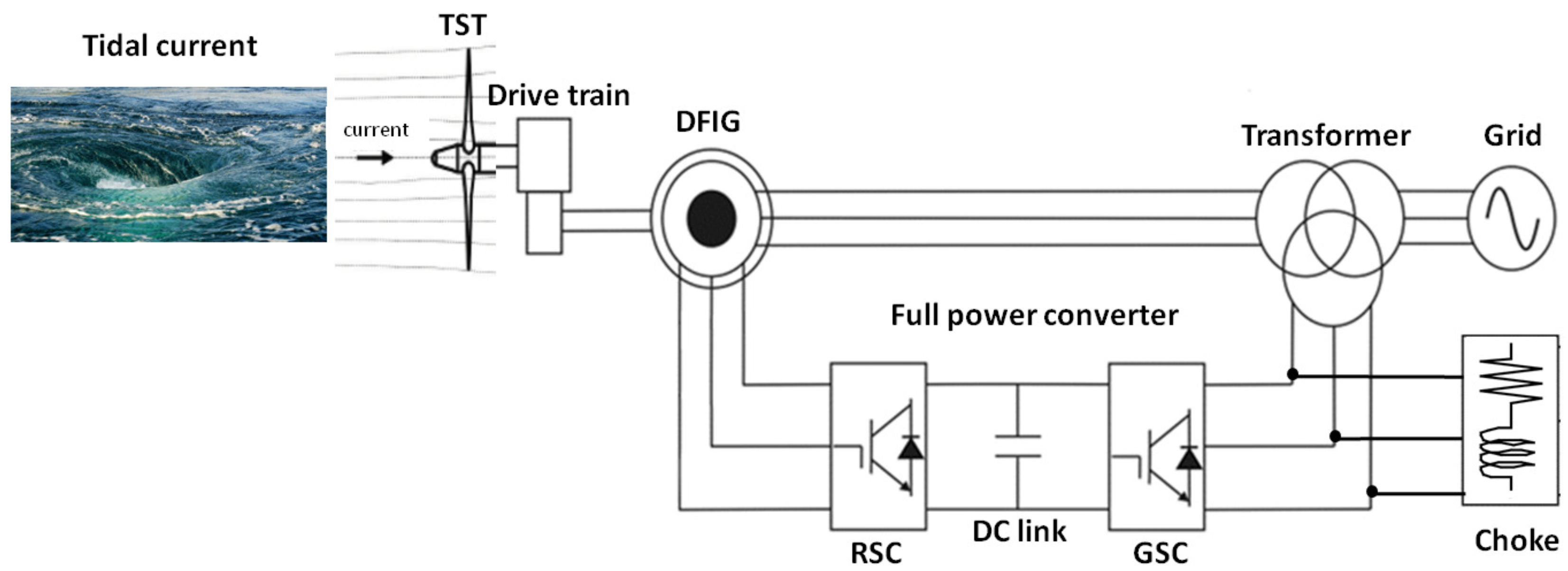
2. Model Statement
2.1. Tidal Turbine Model
2.2. Shaft Model
2.3. DFIG Model
2.4. Back-to-Back Converter Model
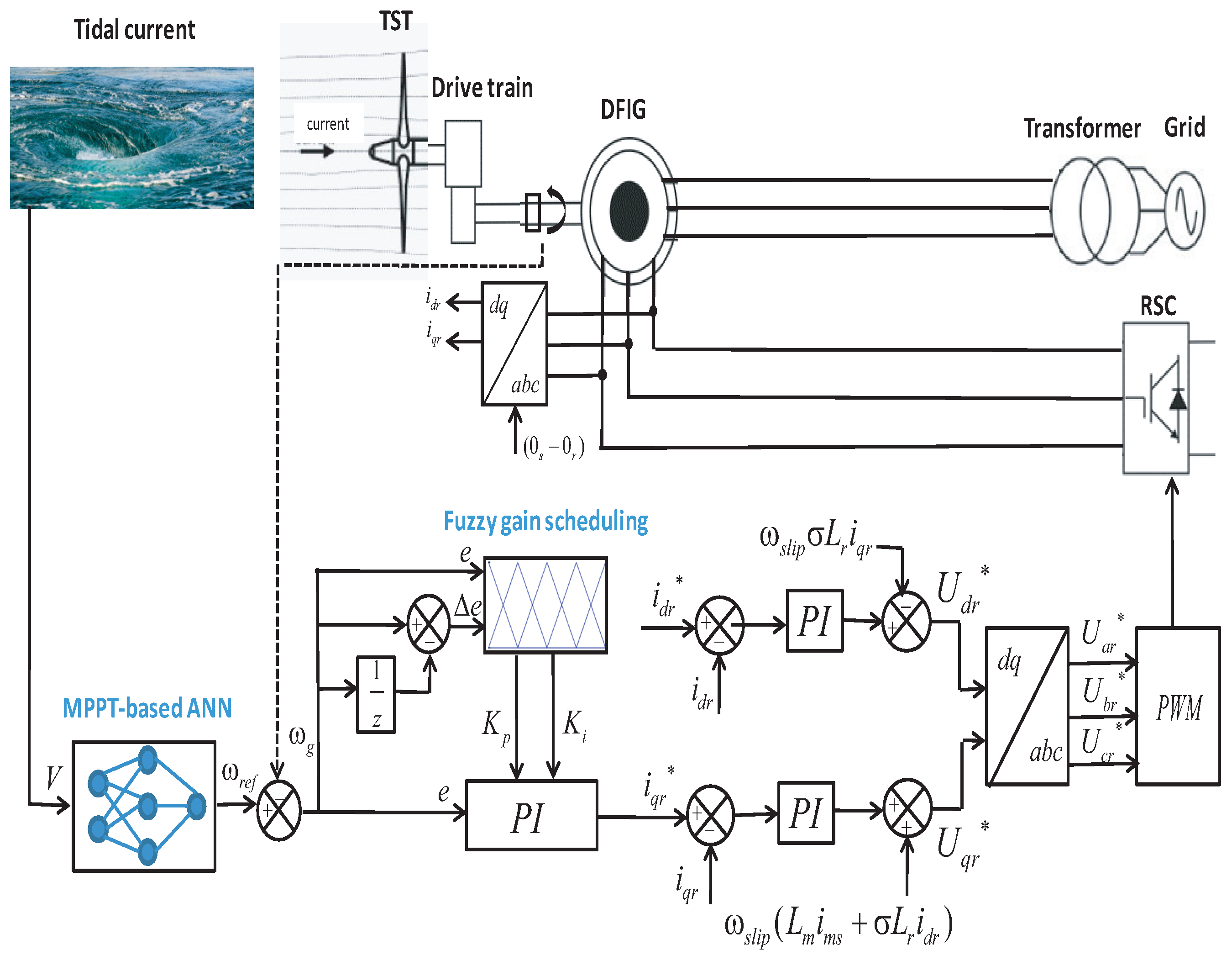
3. Control Statement
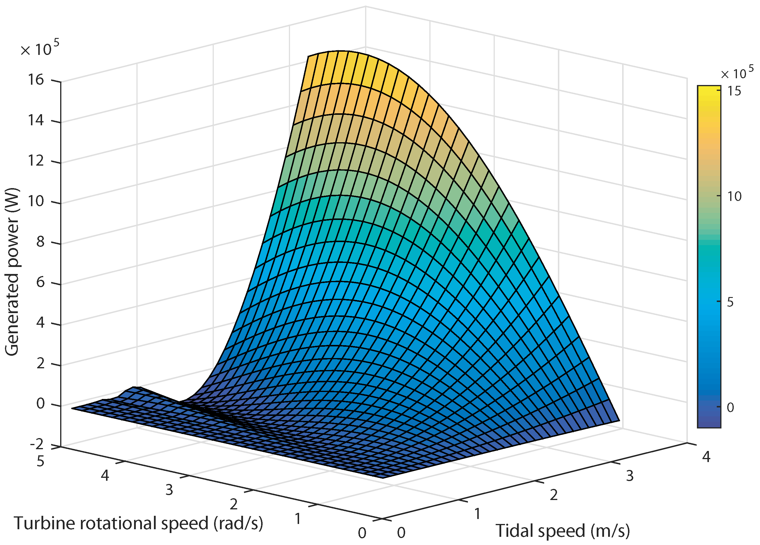
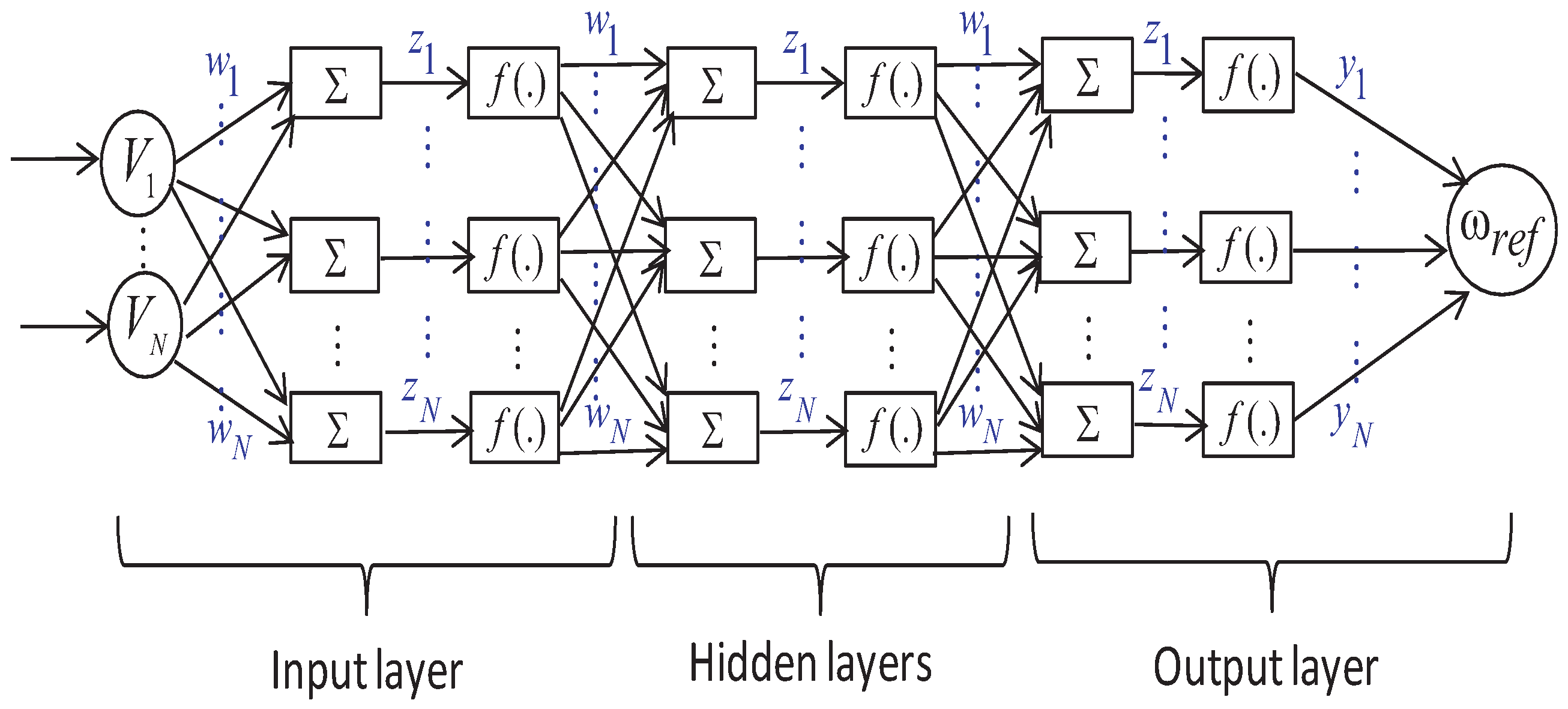
3.1. ANN-Based Maximum Power Point Tracking Approach
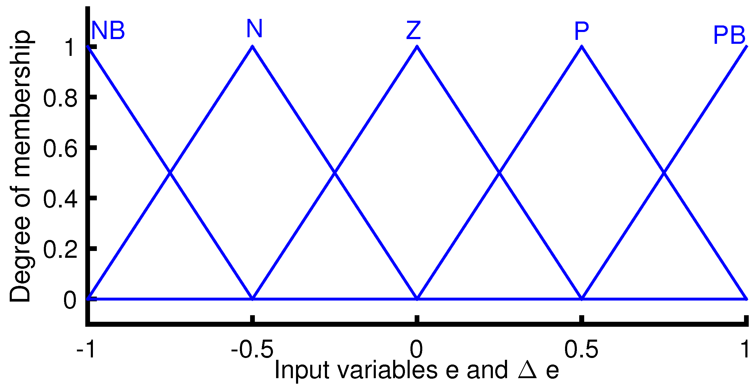
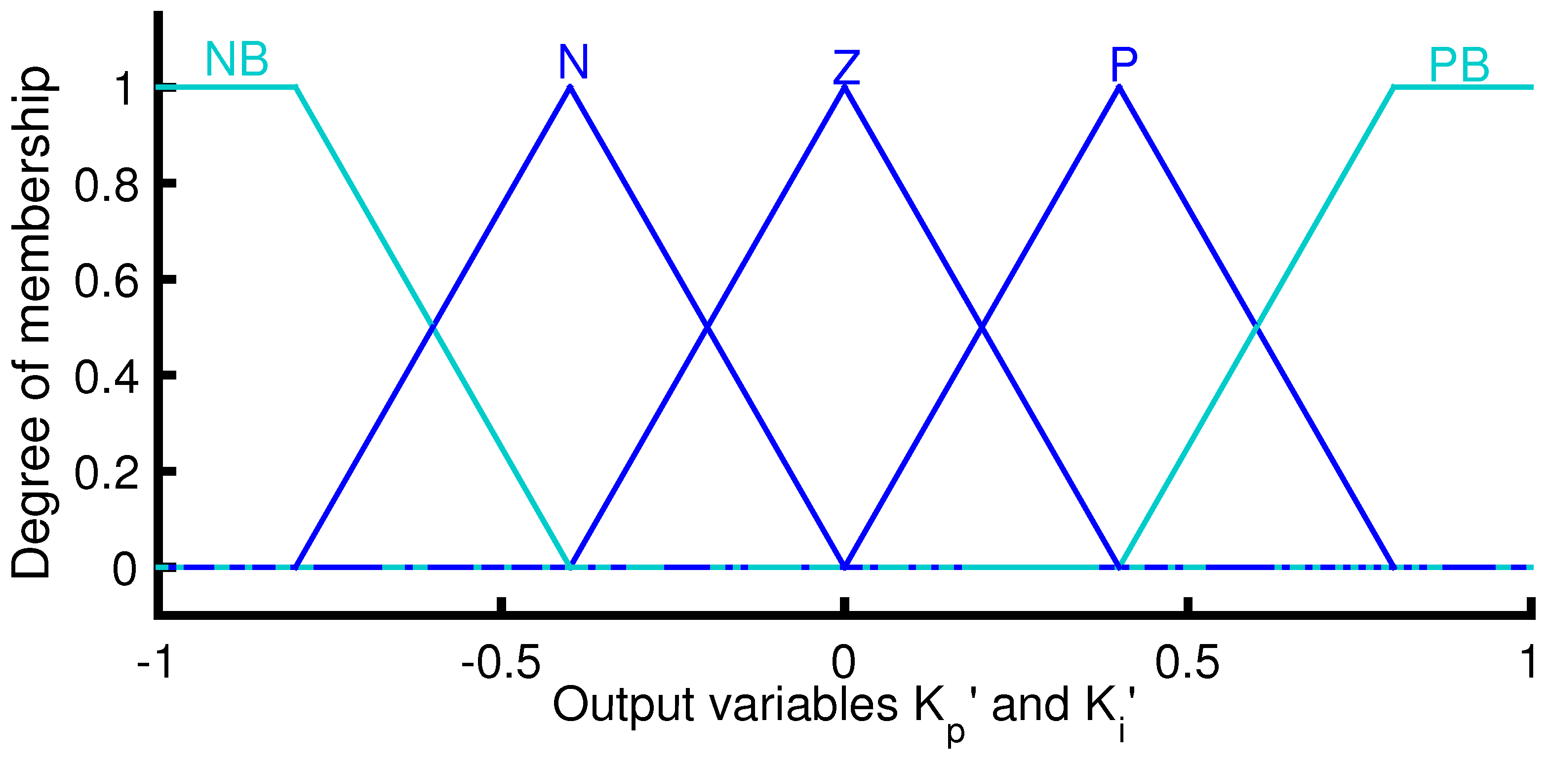
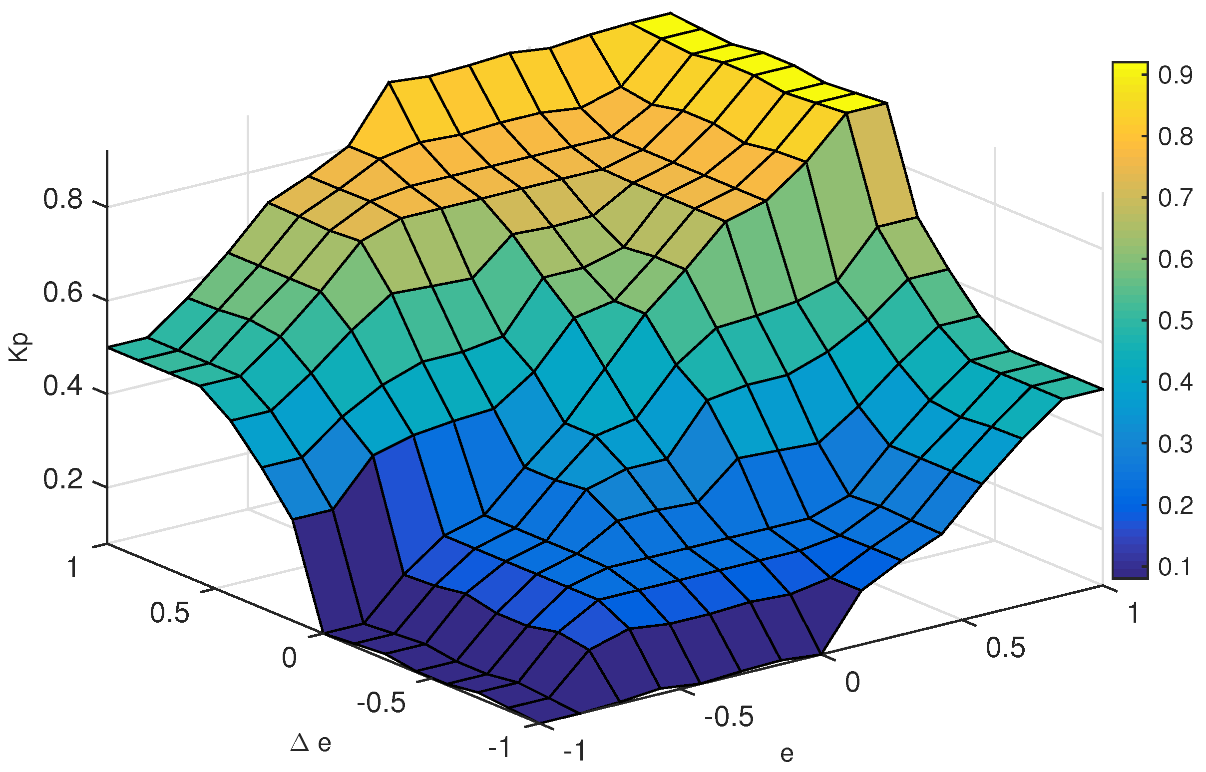
3.2. FGS-PI Based-Rotational Speed Control
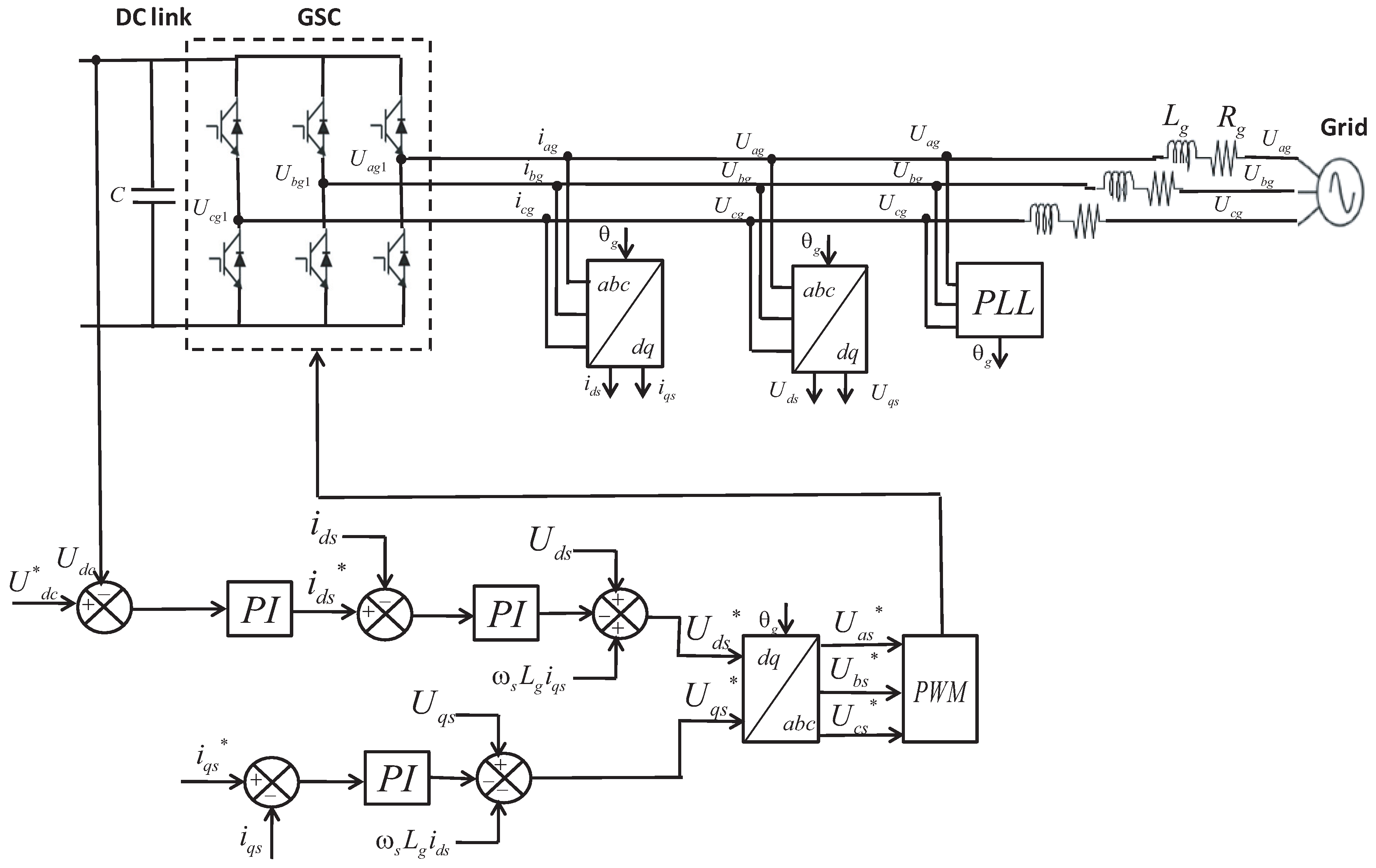
3.3. GSC Control
4. Validation Tests and Discussion
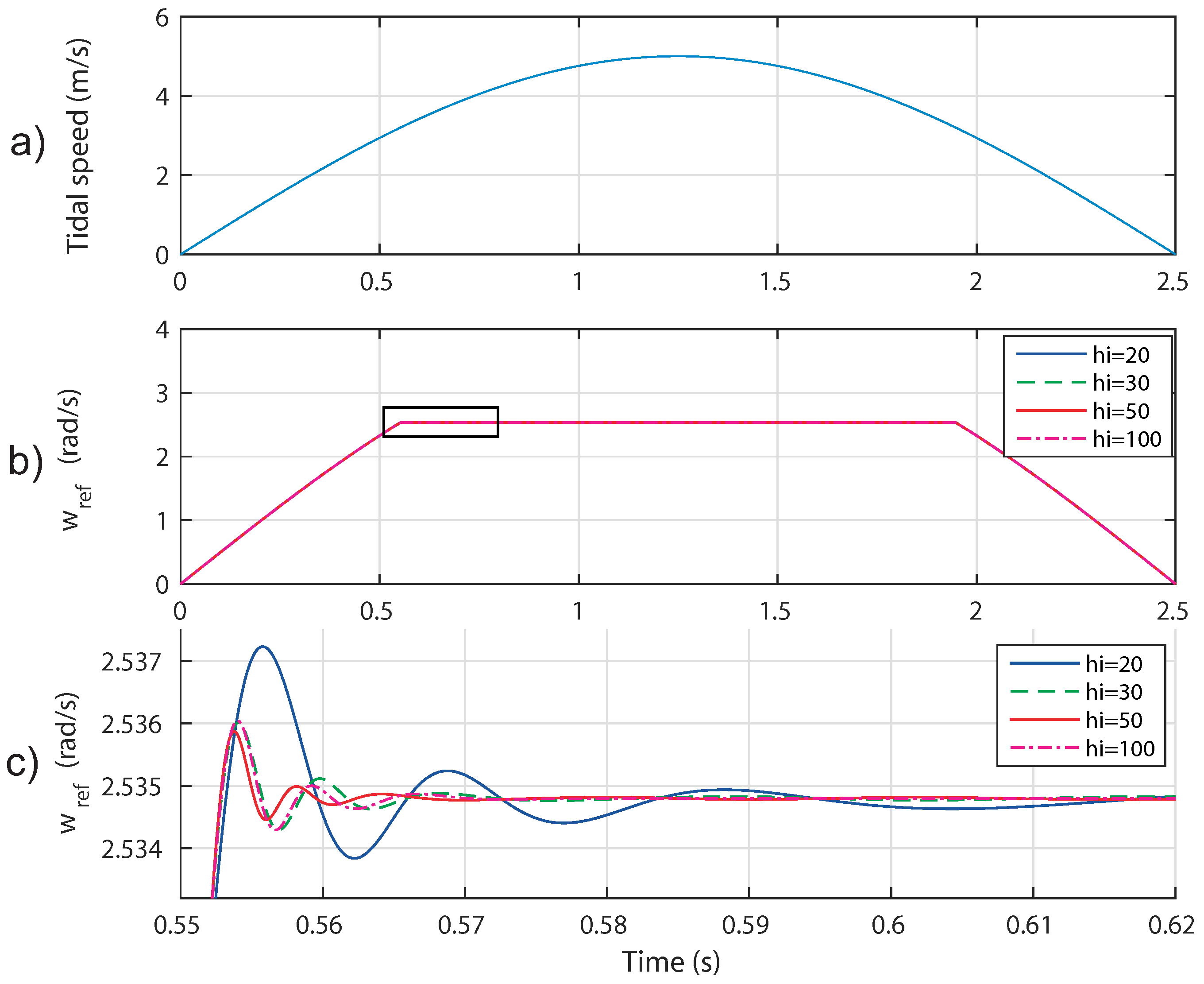
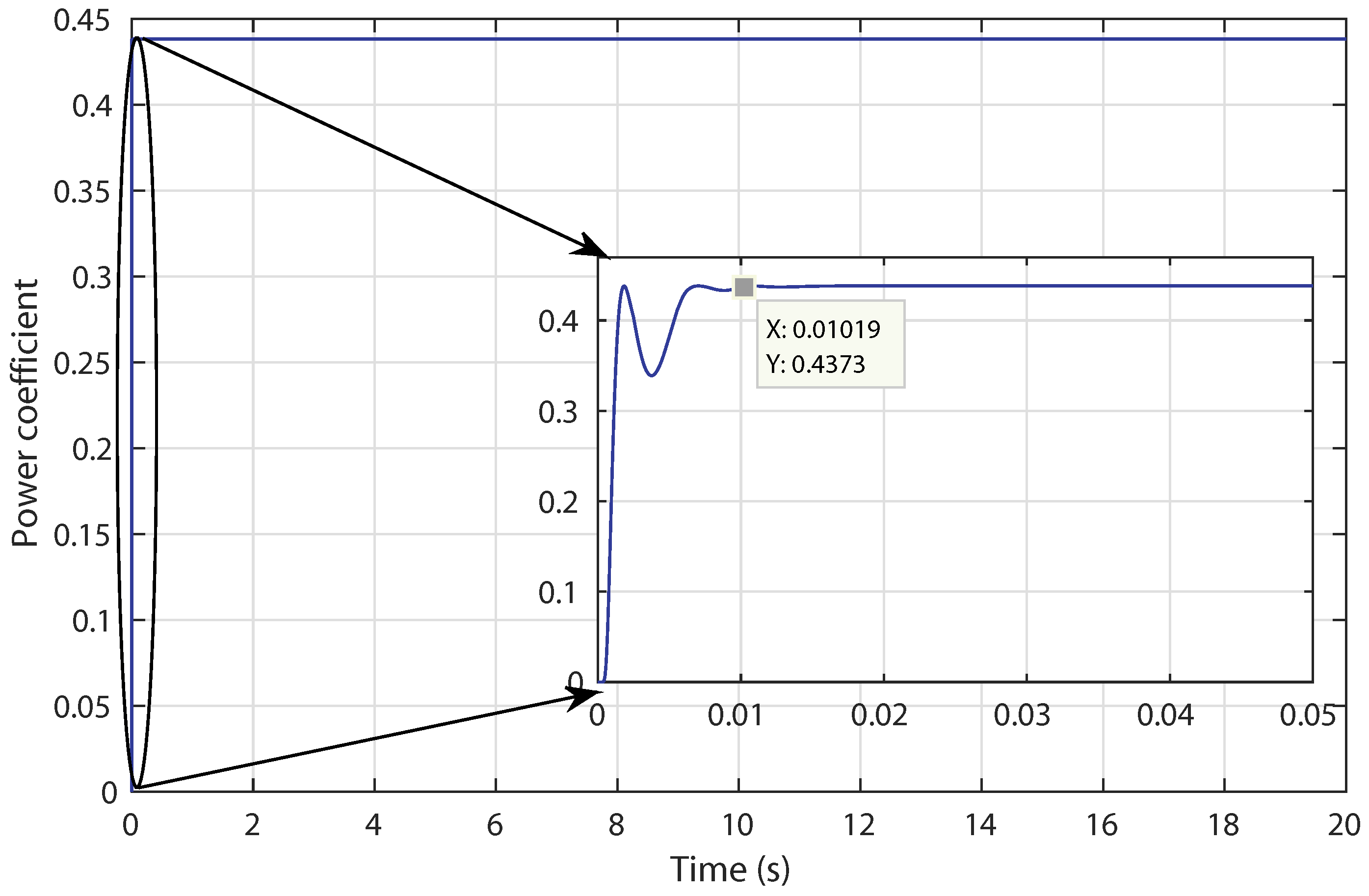
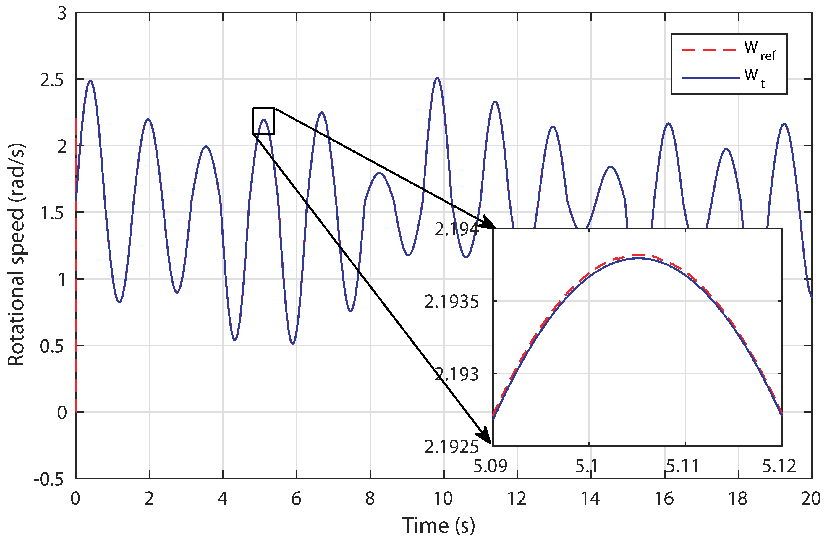
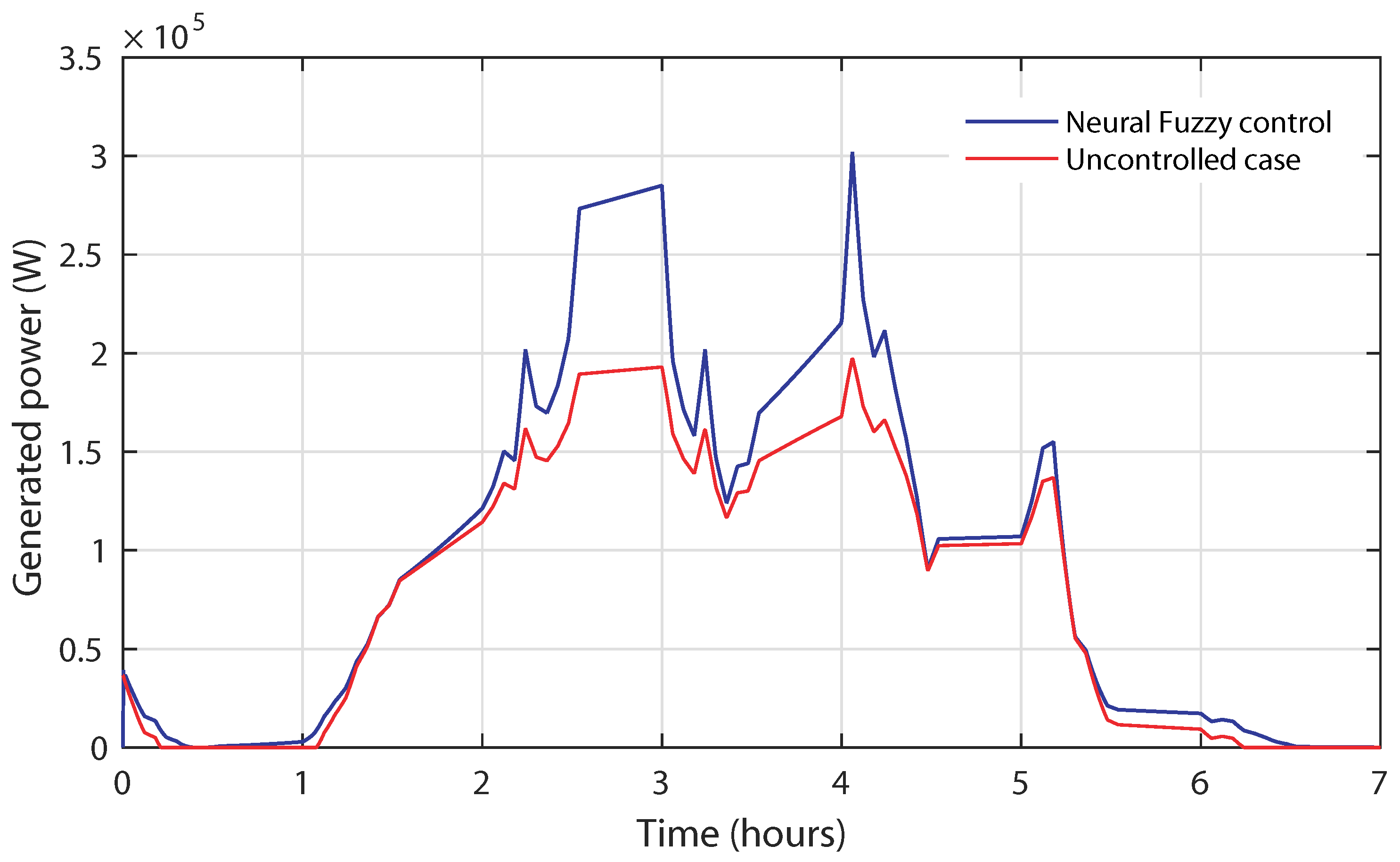
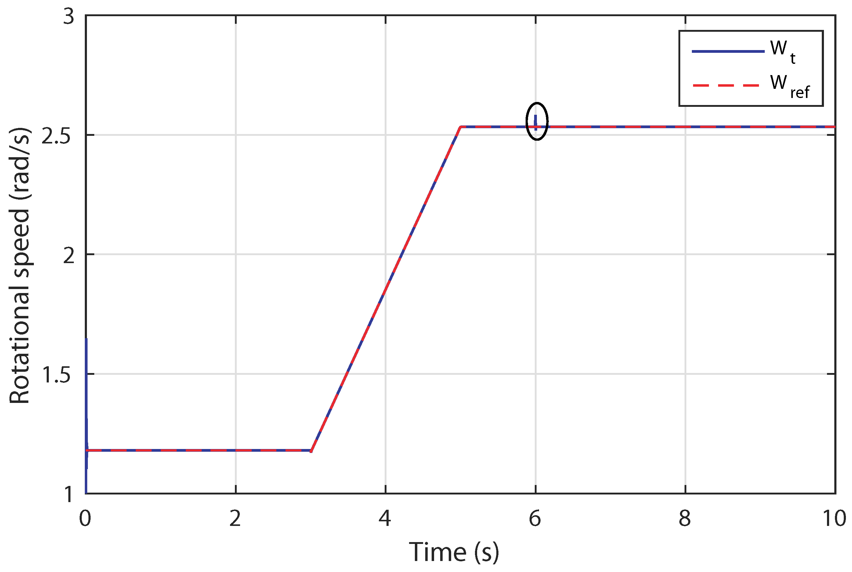
4.1. Control Robustness against Irregular Tidal Speed with Numerical Input
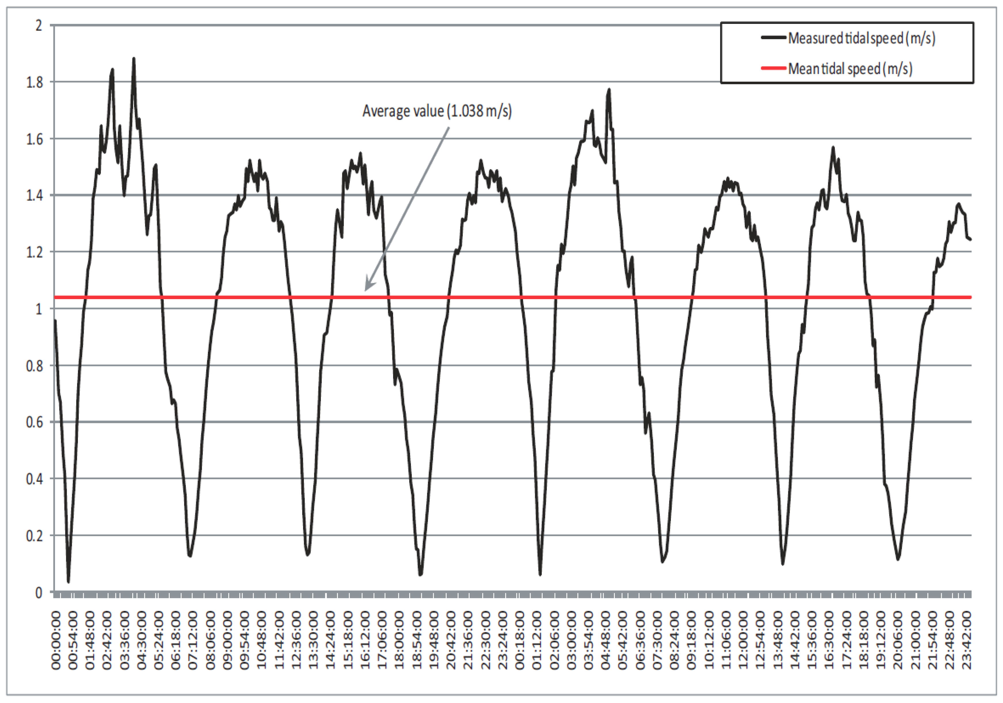
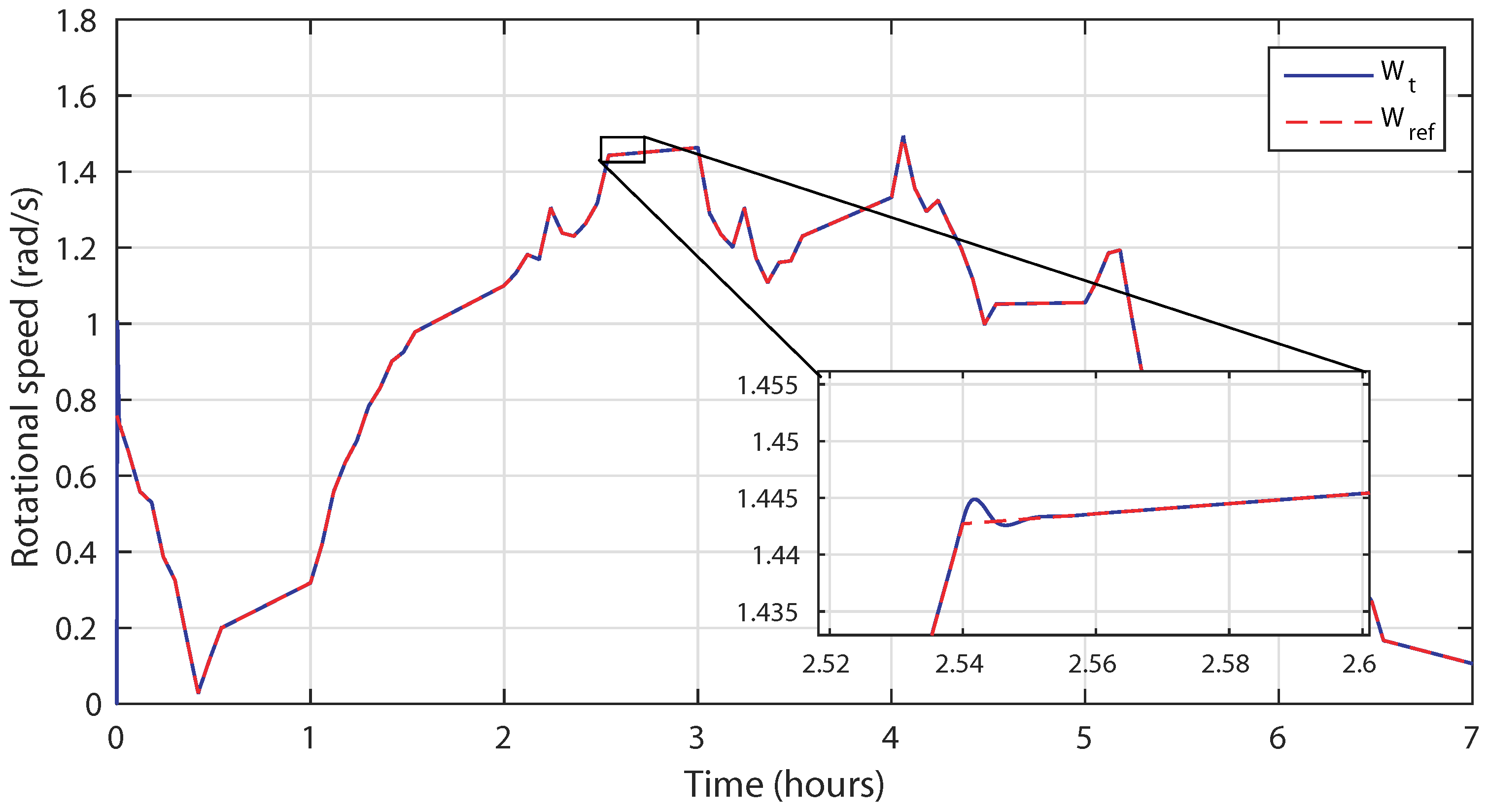
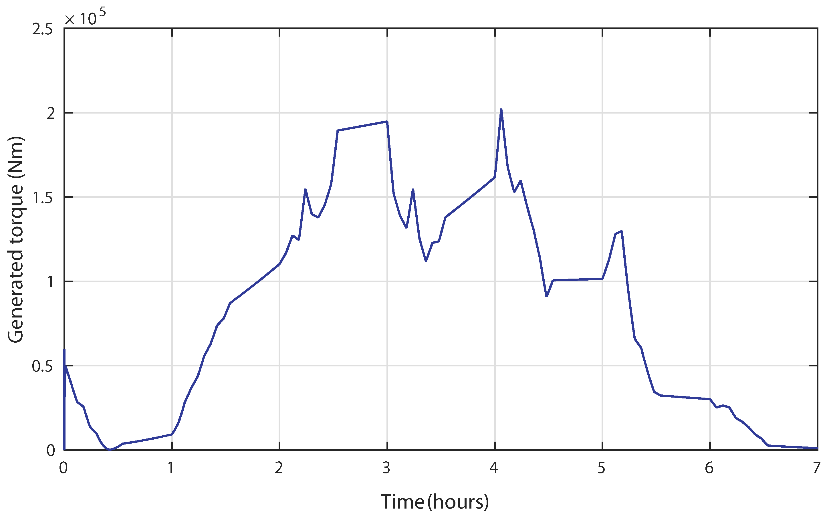
4.2. Control Robustness against Irregular Tidal Speed with Real Measured Input
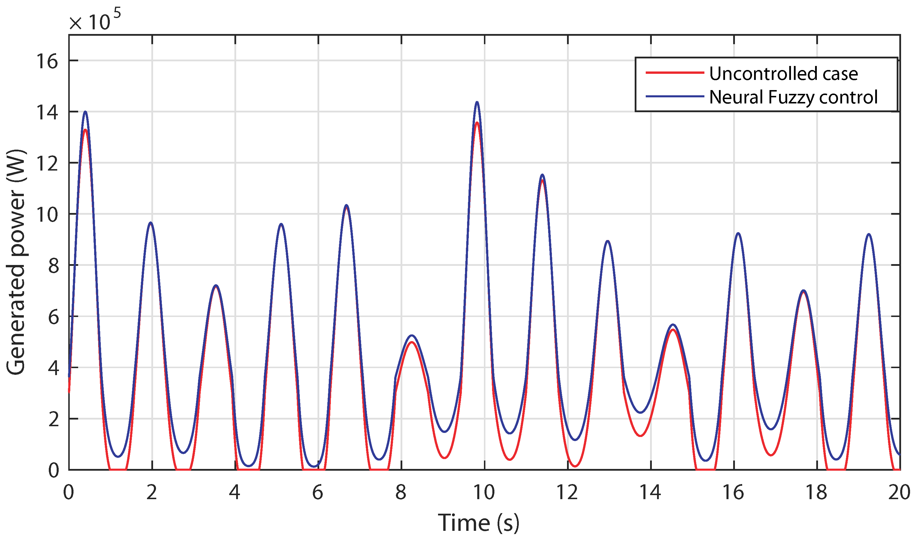
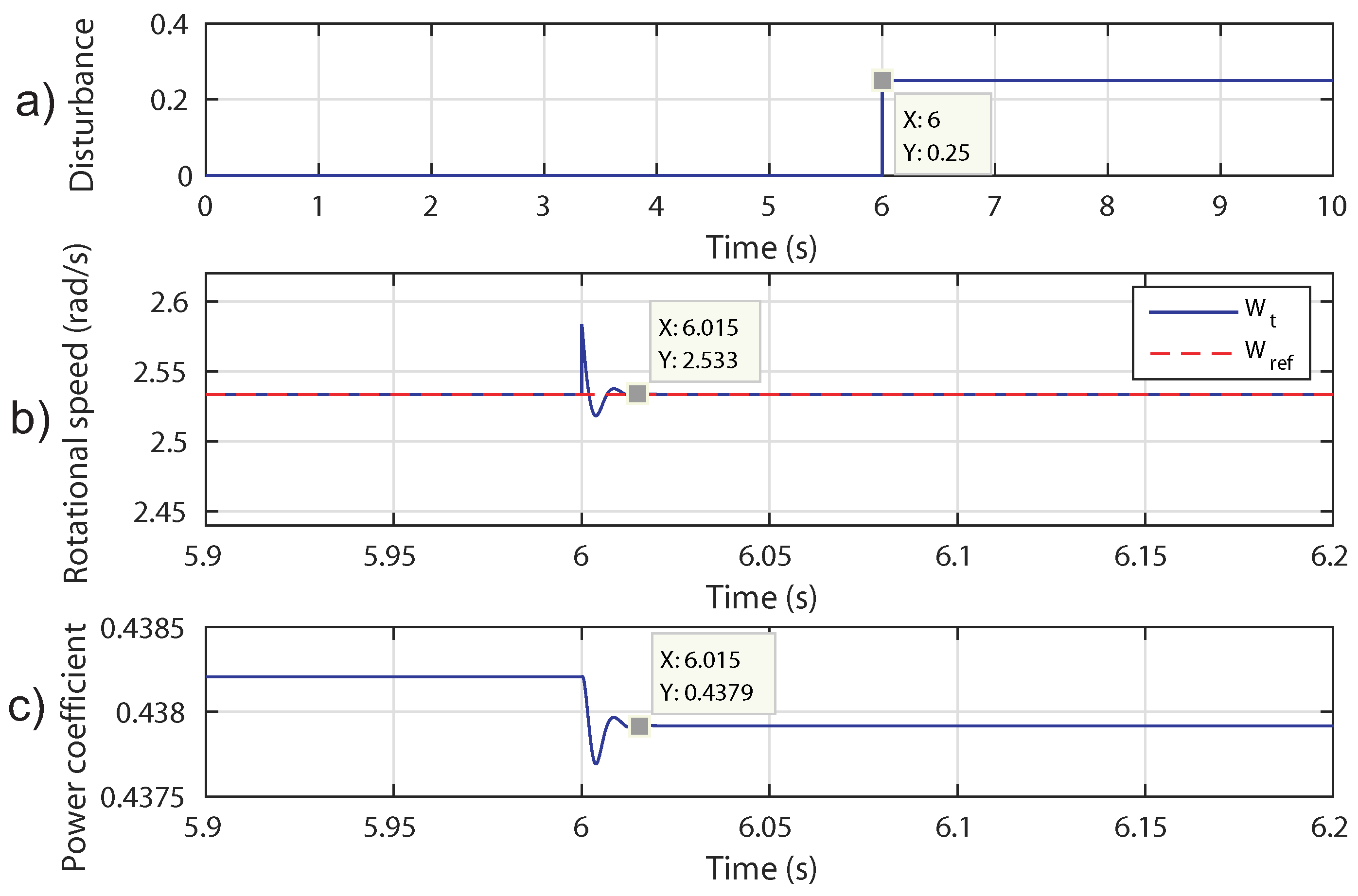
4.3. Disturbance Rejection
5. Conclusions
Author Contributions
Funding
Acknowledgments
Conflicts of Interest
Abbreviations
| ANN | Artificial Neural Network |
| DFIG | Doubly Fed Induction Generator |
| GSC | Grid Side Converter |
| IEA | International Energy Agency |
| FGS | Fuzzy Gain Scheduling |
| IEO | International Energy Outlook |
| MPPT | Maximum Power Point Tracking |
| MSE | Mean Square Error |
| NOAA | National Oceanic and Atmospheric Administration |
| ORC | Optimal Regime Characteristic |
| PI | Proportional Integral |
| PLL | Phase Locked Loop |
| PTO | Power Take Off |
| PWM | Pulse Width Modulation |
| RSC | Rotor Side Converter |
| TSG | Tidal Stream Generator |
| TST | Tidal Stream Turbine |
| NB | Negative Big |
| N | Negative |
| Z | Zero |
| P | Positive |
| PB | Positive Big |
Notations
| Turbine, generator and nominal powers (W). | |
| , | Power coefficient and its maximum. |
| , | Optimal speed ratio and its optimal value. |
| , , R | Blade pitch angle (deg), fluid density (kg/m) and blade radius (m). |
| V, | Tidal current speed and its nominal value (m/s). |
| , | Rotational speed of turbine and generator, pulsations of the stator and rotor (rad/s). |
| Reference rotational speed (rad/s). | |
| , , | Turbine, rotor shaft and electromagnetic torques (Nm). |
| , | Turbine and generator inertia constants, sampling time (s). |
| , , p, | Stiffness coefficient (Nm/rad), damping coefficient (Nms/rad), leakage factor. |
| , p | Angular frequency of slip (rad/s), pole pair numbers. |
| , | Stator and rotor voltages in frame (V). |
| , , | Stator and rotor currents in frame, stator magnetizing current (A). |
| , | Stator and rotor flux in frame (Wb). |
| , , | Stator and rotor inductances, magnetizing inductance, grid coupling inductance (H). |
| , | Stator and rotor resistances, grid coupling resistance . |
| , | Grid voltages and terminal voltages of the converter in frame (V). |
| , | Grid currents in and DC-link current (A). |
| , c | DC-link voltage (V), DC-link capacitor (F). |
| , , | Output neurons, input neurons, threshold terms of the hidden layer. |
| , | synaptic weights, number of neurons in the hidden layer. |
| Fuzzy control law. | |
| , | The error and the error change. |
| , | Fuzzy PI gains. |
| , | Normalized fuzzy PI gains. |
| Grades of the membership functions. |
References
- Segura, E.; Morales, R.; Somolinos, J.A.; Lopez, A. Techno-economic challenges of tidal energy conversion systems: Current status and trends. Renew. Sustain. Energy Rev. 2017, 77, 536–550. [Google Scholar] [CrossRef]
- World Energy Council. World Energy Resource Marine Energy 2016; Technical Report; World Energy Council: London, UK, 2016; pp. 1–76. [Google Scholar]
- Zhang, Y.L.; Lin, Z.; Liu, Q.L. Marine renewable energy in China: Current status and perspectives. Water Sci. Eng. 2014, 7, 288–305. [Google Scholar]
- Grabbe, M.; Lalander, E.; Lundin, S.; Leijon, M. A review of the tidal current energy resource in Norway. Renew. Sustain. Energy Rev. 2009, 13, 1898–1909. [Google Scholar] [CrossRef] [Green Version]
- Kadiri, M.; Ahmadian, R.; Bockelmann-Evans, B.; Rauen, W.; Falconer, R. A review of the potential water quality impacts of tidal renewable energy systems. Renew. Sustain. Energy Rev. 2012, 16, 329–341. [Google Scholar] [CrossRef]
- Stern, N.; Calderon, F. Better Growth, Better Climate: The New Climate Economy Report; The Global Commission on the Economy and Climate: New York, NY, USA, 2014; Available online: http://newclimateeconomy.report/ (accessed on 12 October 2018).
- EIA, U. International Energy Outlook 2016 with Projections to 2040; Energy Department, Energy Information Administration, Office of Energy Analysis: Washington, DC, USA, 2016. [Google Scholar]
- International Energy Agency OECD/IEA. World Energy Outlook 2013, Chapter 6: Renewable Energy Outlook; International Energy Agency OECD/IEA: Paris, France, 2013. [Google Scholar]
- IRENA. REmap 2030: A Renewable Energy Roadmap; IRENA: Dhabi, United Arab Emirates, 2014; Available online: www.irena.org/remap (accessed on 12 October 2018).
- Uihlein, A.; Magagna, D. Wave and tidal current energy—A review of the current state of research beyond technology. Renew. Sustain. Energy Rev. 2016, 58, 1070–1081. [Google Scholar] [CrossRef]
- Borthwick, A.G. Marine renewable energy seascape. Engineering 2016, 2, 69–78. [Google Scholar] [CrossRef]
- Garrido, A.J.; Garrido, I.; Otaola, E.; Lekube, J.; MZoughi, F.; Ghefiri, K.; Mundackamattam, D.G.; Oleagordia, I. Capture chamber modelling and validation in OWC on-shore devices. In Proceedings of the Region 10 Conference (TENCON), Singapore, 22–25 November 2016; pp. 1682–1685. [Google Scholar]
- El Tawil, T.; Charpentier, J.F.; Benbouzid, M. Tidal energy site characterization for marine turbine optimal installation: Case of the Ouessant Island in France. Int. J. Mar. Energy 2017, 18, 57–64. [Google Scholar] [CrossRef]
- Bryden, I.G.; Couch, S.J. ME1-marine energy extraction: Tidal resource analysis. Renew. Energy 2006, 31, 133–139. [Google Scholar] [CrossRef]
- Myers, L.; Bahaj, A.S. Simulated electrical power potential harnessed by marine current turbine arrays in the Alderney Race. Renew. Energy 2005, 30, 1713–1731. [Google Scholar] [CrossRef]
- Winter, A.I. Differences in fundamental design drivers for wind and tidal turbines. In Proceedings of the 2011 IEEE-Spain OCEANS, Santander, Spain, 6–9 June 2011; pp. 1–10. [Google Scholar]
- Whitby, B.; Ugalde-Loo, C.E. Performance of pitch and stall regulated tidal stream turbines. IEEE Trans. Sustain. Energy 2014, 5, 64–72. [Google Scholar] [CrossRef]
- Hammons, T.J. Tidal power. Proc. IEEE 1993, 81, 419–433. [Google Scholar] [CrossRef]
- Choi, J.S.; Jeong, R.G.; Shin, J.H.; Kim, C.K.; Kim, Y.S. New Control Method of Maximum Power Point Tracking for Tidal Energy Generation System. In Proceedings of the International Conference on Electrical Machines and Systems, Seoul, Korea, 8–11 October 2007; pp. 165–168. [Google Scholar]
- Rahman, M.L.; Oka, S.; Shirai, Y. Hybrid power generation system using offshore-wind turbine and tidal turbine for power fluctuation compensation (HOT-PC). IEEE Trans. Sustain. Energy 2010, 1, 92–98. [Google Scholar] [CrossRef]
- Xiang, D.; Ran, L.; Tavner, P.J.; Yang, S. Control of a doubly fed induction generator in a wind turbine during grid fault ride-through. IEEE Trans. Energy Convers. 2006, 21, 652–662. [Google Scholar] [CrossRef]
- Sousounis, M.C.; Shek, J.K.H.; Mueller, M.A. Modelling and control of tidal energy conversion systems with long distance converters. In Proceedings of the 7th IET International Conference on Power Electronics, Machines and Drives (PEMD 2014), Manchester, UK, 8–10 April 2014; pp. 1–6. [Google Scholar]
- Munteanu, I.; Bratcu, A.L.; Cutululis, N.A.; Ceanga, E. Optimal Control of Wind Energy Systems: Towards a Global Approach; Springer: Berlin, Germany, 2008. [Google Scholar]
- Marzband, M.; Azarinejadian, F.; Savaghebi, M.; Pouresmaeil, E.; Guerrero, J.M.; Lightbody, G. Smart transactive energy framework in grid-connected multiple home microgrids under independent and coalition operations. Renew. Energy 2018, 126, 95–106. [Google Scholar] [CrossRef]
- Tavakoli, M.; Shokridehaki, F.; Marzband, M.; Godina, R.; Pouresmaeil, E. A Two Stage Hierarchical Control Approach for the Optimal Energy Management in Commercial Building Microgrids Based on Local Wind Power and PEVs. Sustain. Cities Soc. 2018, 41, 332–340. [Google Scholar] [CrossRef]
- Utkin, V.I. Sliding Modes in Control and Optimization; Springer: Berlin, Germany, 1992. [Google Scholar]
- Elghali, S.E.B.; Benbouzid, M.E.H.; Charpentier, J.F.; Ahmed-Ali, T.; Munteanu, I. Experimental Validation of a Marine Current Turbine Simulator: Application to a Permanent Magnet Synchronous Generator-Based System Second-Order Sliding Mode Control. IEEE Trans. Ind. Electron. 2011, 58, 118–126. [Google Scholar] [Green Version]
- Feng, Y.; Han, F.; Yu, X. Chattering free full-order sliding-mode control. Automatica 2014, 50, 1310–1314. [Google Scholar] [CrossRef]
- Kalogirou, S.A. Artificial neural networks in renewable energy systems applications: A review. Renew. Sustain. Energy Rev. 2001, 5, 373–401. [Google Scholar] [CrossRef]
- Morgan, N.; Bourlard, H.A. Neural networks for statistical recognition of continuous speech. Proc. IEEE 1995, 83, 742–772. [Google Scholar] [CrossRef]
- Bilgili, M.; Sahin, B.; Yasar, A. Application of artificial neural networks for the wind speed prediction of target station using reference stations data. Renew. Energy 2007, 32, 2350–2360. [Google Scholar] [CrossRef]
- Castro, A.; Carballo, R.; Iglesias, G.; Rabunal, J.R. Performance of artificial neural networks in nearshore wave power prediction. Appl. Soft Comput. 2014, 23, 194–201. [Google Scholar] [CrossRef]
- Dounis, A.I.; Kofinas, P.; Alafodimos, C.; Tseles, D. Adaptive fuzzy gain scheduling PID controller for maximum power point tracking of photovoltaic system. Renew. Energy 2013, 60, 202–214. [Google Scholar] [CrossRef]
- Chaiyatham, T.; Ngamroo, I. Optimal fuzzy gain scheduling of PID controller of superconducting magnetic energy storage for power system stabilization. Int. J. Innov. Comput. Inf. Control 2013, 9, 651–666. [Google Scholar]
- Bahaj, A.S.; Molland, A.F.; Chaplin, J.R.; Batten, W.M.J. Power and thrust measurements of marine current turbines under various hydrodynamic flow conditions in a cavitation tunnel and a towing tank. Renew. Energy 2007, 32, 407–426. [Google Scholar] [CrossRef]
- Ghefiri, K.; Bouallègue, S.; Garrido, I.; Garrido, A.J.; Haggège, J. Complementary Power Control for Doubly Fed Induction Generator-Based Tidal Stream Turbine Generation Plants. Energies 2017, 10, 862. [Google Scholar] [CrossRef]
- Ghefiri, K.; Bouallègue, S.; Haggège, J. Modeling and SIL simulation of a Tidal Stream device for marine energy conversion. In Proceedings of the 2015 6th International Renewable Energy Congress (IREC), Sousse, Tunisia, 24–26 March 2015; pp. 1–6. [Google Scholar]
- Muljadi, E.; Gevorgian, V.; Wright, A.; Donegan, J.; Marnagh, C.; McEntee, J. Turbine Control of a Tidal and River Power Generator: Preprint (No. NREL/CP-5D00-66867); National Renewable Energy Lab.(NREL): Golden, CO, USA, 2016. [Google Scholar]
- Fernandez, L.M.; Jurado, F.; Saenz, J.R. Aggregated dynamic model for wind farms with doubly fed induction generator wind turbines. Renew. Energy 2008, 33, 129–140. [Google Scholar] [CrossRef]
- Benelghali, S.; Benbouzid, M.E.H.; Charpentier, J.F. Generator systems for marine current turbine applications: A comparative study. IEEE J. Ocean. Eng. 2012, 37, 554–563. [Google Scholar] [CrossRef] [Green Version]
- Amundarain, M.; Alberdi, M.; Garrido, A.J.; Garrido, I. Modeling and simulation of wave energy generation plants: Output power control. IEEE Trans. Ind. Electron. 2011, 58, 105–117. [Google Scholar] [CrossRef]
- Fan, L.; Kavasseri, R.; Miao, Z.L.; Zhu, C. Modeling of DFIG-based wind farms for SSR analysis. IEEE Trans. Power Deliv. 2010, 25, 2073–2082. [Google Scholar] [CrossRef]
- Pena, R.; Clare, J.C.; Asher, G.M. Doubly fed induction generator using back-to-back PWM converters and its application to variable-speed wind-energy generation. IEE Proc.-Electr. Power Appl. 1996, 143, 231–241. [Google Scholar] [CrossRef]
- Zhou, D.; Blaabjerg, F.; Lau, M.; Tonnes, M. Optimized reactive power flow of DFIG power converters for better reliability performance considering grid codes. IEEE Trans. Ind. Electron. 2015, 62, 1552–1562. [Google Scholar] [CrossRef]
- Muller, S.; Deicke, M.; De Doncker, R.W. Doubly fed induction generator systems for wind turbines. IEEE Ind. Appl. Mag. 2002, 8, 26–33. [Google Scholar] [CrossRef]
- Alberdi, M.; Amundarain, M.; Garrido, A.J.; Garrido, I.; Casquero, O.; De la Sen, M. Complementary control of oscillating water column-based wave energy conversion plants to improve the instantaneous power output. IEEE Trans. Energy Convers. 2011, 26, 1021–1032. [Google Scholar] [CrossRef]
- Rizzo, S.A.; Scelba, G. ANN based MPPT method for rapidly variable shading conditions. Appl. Energy 2015, 145, 124–132. [Google Scholar] [CrossRef]
- Makarynskyy, O.; Makarynska, D.; Rusu, E.; Gavrilov, A. Filling gaps in wave records with artificial neural networks. Marit. Transp. Exploit. Ocean Coast. Resour. 2005, 2, 1085–1091. [Google Scholar]
- Ghefiri, K.; Bouallègue, S.; Garrido, I.; Garrido, A.J.; Haggège, J. Modeling and MPPT control of a Tidal Stream Generator. In Proceedings of the 2017 4th International Conference on Control, Decision and Information Technologies (CoDIT’17), Barcelona, Spain, 5–7 April 2017; pp. 1003–1008. [Google Scholar]
- Hagan, M.T.; Menhaj, M.B. Training feedforward networks with the Marquardt algorithm. IEEE Trans. Neural Netw. 1994, 5, 989–993. [Google Scholar] [CrossRef] [PubMed]
- Wilamowski, B.M.; Yu, H. Improved computation for Levenberg-Marquardt training. IEEE Trans. Neural Netw. 2010, 21, 930–937. [Google Scholar] [CrossRef] [PubMed]
- Lewis, M.J.; Neill, S.P.; Hashemi, M.R.; Reza, M. Realistic wave conditions and their influence on quantifying the tidal stream energy resource. Appl. Energy 2014, 136, 495–508. [Google Scholar] [CrossRef]
- Zhao, Z.Y.; Tomizuka, M.; Isaka, S. Fuzzy gain scheduling of PID controllers. IEEE Trans. Syst. Man Cybern. 1993, 23, 1392–1398. [Google Scholar] [CrossRef]
- Tursini, M.; Parasiliti, F.; Zhang, D. Real-time gain tuning of PI controllers for high-performance PMSM drives. IEEE Trans. Ind. Appl. 2002, 38, 1018–1026. [Google Scholar] [CrossRef]
- Bouallègue, S.; Haggège, J.; Ayadi, M.; Benrejeb, M. PID-type fuzzy logic controller tuning based on particle swarm optimization. Eng. Appl. Artif. Intell. 2012, 25, 484–493. [Google Scholar] [CrossRef]
- Chen, Y.Y.; Perng, C.F. Input scaling factors in fuzzy control systems. In Proceedings of the 1994 3rd International Fuzzy Systems Conference, Orlando, FL, USA, 26–29 June 1994; pp. 1666–1670. [Google Scholar]
- Bedoud, K.; Ali-rachedi, M.; Bahi, T.; Lakel, R. Adaptive fuzzy gain scheduling of PI controller for control of the wind energy conversion systems. Energy Procedia 2015, 74, 211–225. [Google Scholar] [CrossRef]
- Qu, L.; Qiao, W. Constant power control of DFIG wind turbines with supercapacitor energy storage. IEEE Trans. Ind. Appl. 2011, 47, 359–367. [Google Scholar] [CrossRef]
- Astrom, K.J.; Hagglund, T. Advanced Pid Control; ISA-The Instrumentation, Systems, and Automation Society: Research Triangle Park, NC, USA, 2006. [Google Scholar]
- Vilanova, R.; Visioli, A. PID Control in the Third Millennium; Springer: London, UK, 2012. [Google Scholar]
- Blaabjerg, F.; Teodorescu, R.; Liserre, M.; Timbus, A.V. Overview of control and grid synchronization for distributed power generation systems. IEEE Trans. Ind. Electron. 2006, 53, 1398–1409. [Google Scholar] [CrossRef]
- Zhou, Z.; Benbouzid, M.; Charpentier, J.F.; Scuiller, F.; Tang, T. A review of energy storage technologies for marine current energy systems. Renew. Sustain. Energy Rev. 2013, 18, 390–400. [Google Scholar] [CrossRef] [Green Version]
- Alves, J.H.G. Numerical modeling of ocean swell contributions to the global wind-wave climate. Ocean Model. 2006, 11, 98–122. [Google Scholar] [CrossRef]
- National Oceanic and Atmospheric Administration (NOAA). Available online: https://tidesandcurrents.noaa.gov/ (accessed on 30 March 2018).[Green Version]
- Kostaschuk, R.; Best, J.; Villard, P.; Peakall, J.; Franklin, M. Measuring flow velocity and sediment transport with an acoustic Doppler current profiler. Geomorphology 2005, 68, 25–37. [Google Scholar] [CrossRef]


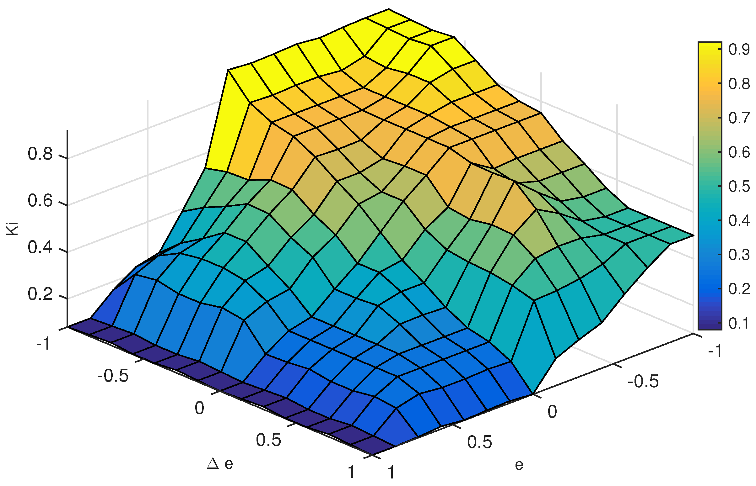
| NB | N | Z | P | PB | |
|---|---|---|---|---|---|
| NB | NB | NB | NB | N | Z |
| N | NB | N | N | N | Z |
| Z | NB | N | Z | P | PB |
| P | Z | P | P | P | PB |
| PB | Z | P | PB | PB | PB |
| NB | N | Z | P | PB | |
|---|---|---|---|---|---|
| NB | PB | PB | PB | N | NB |
| N | PB | P | P | Z | NB |
| Z | P | P | Z | N | NB |
| P | Z | P | N | N | NB |
| PB | Z | N | NB | NB | NB |
| Turbine | Drive-train | DFIG | Converter |
|---|---|---|---|
| kg/m | s | MW | V |
| m | s | V | F |
| Nm/rad | Hz | ||
| Nms/rad | m | ||
| m/s | m | Choke | |
| mH | m | ||
| mH | mH | ||
| mH | |||
© 2018 by the authors. Licensee MDPI, Basel, Switzerland. This article is an open access article distributed under the terms and conditions of the Creative Commons Attribution (CC BY) license (http://creativecommons.org/licenses/by/4.0/).
Share and Cite
Ghefiri, K.; Garrido, I.; Bouallègue, S.; Haggège, J.; Garrido, A.J. Hybrid Neural Fuzzy Design-Based Rotational Speed Control of a Tidal Stream Generator Plant. Sustainability 2018, 10, 3746. https://0-doi-org.brum.beds.ac.uk/10.3390/su10103746
Ghefiri K, Garrido I, Bouallègue S, Haggège J, Garrido AJ. Hybrid Neural Fuzzy Design-Based Rotational Speed Control of a Tidal Stream Generator Plant. Sustainability. 2018; 10(10):3746. https://0-doi-org.brum.beds.ac.uk/10.3390/su10103746
Chicago/Turabian StyleGhefiri, Khaoula, Izaskun Garrido, Soufiene Bouallègue, Joseph Haggège, and Aitor J. Garrido. 2018. "Hybrid Neural Fuzzy Design-Based Rotational Speed Control of a Tidal Stream Generator Plant" Sustainability 10, no. 10: 3746. https://0-doi-org.brum.beds.ac.uk/10.3390/su10103746