Article

Long-Term Decision on Wind Investment with Considering Different Load Ranges of Power Plant for Sustainable Electricity Energy Market

by
Jaber Valinejad
1,
Mousa Marzband
2,3,
Mudathir Funsho Akorede
4,
Ian D Elliott
2,
Radu Godina
5,
João Carlos de Oliveira Matias
6,7 and
Edris Pouresmaeil
8,*
1
Bradley Department of Electrical and Computer Engineering, Virginia Tech, Northern Virginia Center, Falls Church, VA 24043, USA
2
Department of Physics and Electrical Engineering, Faculty of Engineering and Environment, Northumbria University Newcastle, Newcastle upon Tyne NE18ST, UK
3
Department of Electrical Engineering, Lahijan Branch, Islamic Azad University, Lahijan 4416939515, Iran
4
Department of Electrical & Electronics Engineering, Faculty of Engineering and Technology, University of Ilorin, P.M.B. 1515, Ilorin 240003, Nigeria
5
Centre for Aerospace Science and Technologies—Department of Electromechanical Engineering, University of Beira Interior, 6201-001 Covilhã, Portugal
6
DEGEIT—Department of Economics, Management, Industrial Engineering and Tourism, University of Aveiro, 3810-193 Aveiro, Portugal
7
GOVCOPP—Research Unit on Governance, Competitiveness and Public Policies, University of Aveiro, 3810-193 Aveiro, Portugal
8
Department of Electrical Engineering and Automation, Aalto University, 02150 Espoo, Finland
*
Author to whom correspondence should be addressed.
Sustainability 2018, 10(10), 3811; https://0-doi-org.brum.beds.ac.uk/10.3390/su10103811
Submission received: 23 September 2018 / Revised: 10 October 2018 / Accepted: 15 October 2018 / Published: 22 October 2018
(This article belongs to the Special Issue Sustainable Energy Systems: From Primary to End-Use)

Abstract

:
The aim of this paper is to provide a bi-level model for the expansion planning on wind investment while considering different load ranges of power plants in power systems at a multi-stage horizon. Different technologies include base load units, such as thermal and water units, and peak load units such as gas turbine. In this model, subsidies are considered as a means to encourage investment in wind turbines. In order that the uncertainties related to demand and the wind turbine can be taken into consideration, these effects are modelled using a variety of scenarios. In addition, the load demand is characterized by a certain number of demand blocks. The first-level relates to the issue of investment in different load ranges of power plants with a view to maximizing the investment profit whilst the second level is related to the market-clearing where the priority is to maximize the social welfare benefits. The bi-level optimization problem is then converted to a dynamic stochastic mathematical algorithm with equilibrium constraint (MPEC) and represented as a mixed integer linear program (MILP) after linearization. The proposed framework is examined on a real transmission network. Simulation results confirm that the proposed framework can be a useful tool for analyzing the investments different load ranges of power plants on long-term strategic decision-making.

1. Introduction

Investment in renewable energy sources, including wind power plant, is of particular importance due to the increase in the efficiency of clean energy, and the need to reduce pollution and fuel consumption [1,2,3]. However, the production of wind resourced units involves an inherent uncertainty and limited capacity, which alone may not be responsible for load growth in a power grid [4,5,6,7]. In addition, investment in wind resources may be less profitable than other technologies for investor due to budget constraints [8,9,10,11,12]. Consequently, there is a need to pay special attention to investing in renewable energy, including wind power, when carrying out generation expansion planning. Moreover, the possibility of investing in other technologies are taken into account in the model when generation expansion planning (GEP) is undertaken. However, this issue in previously presented models is often overlooked.
On the other hand, the analysis of the dynamic approach to this problem is of great importance due to the fact that yearly investment decisions (including capacity, location and time of construction) depend on investment decisions carried out in previous years [13,14,15,16,17]. As a result, in this article, we focus on a dynamic approach including renewable energy such as wind power in the grid used in the highest possible value. For this reason, investors will be encouraged to invest in the units while giving consideration to subsidies for new wind units. Whilst it is possible that the above incentives may not result in investment, other technologies that exploit peak load and base load units that consider various aspects (such as budget constraints, uncertainty and the limited capacity of wind turbines, etc.) during the planning stages, may be more profitable and therefore more attractive to investors.
In Figure 1, the effectiveness of the proposed GEP model is shown along with the above studies’ shortcomings. The following points outline the important research that has been done in this field:
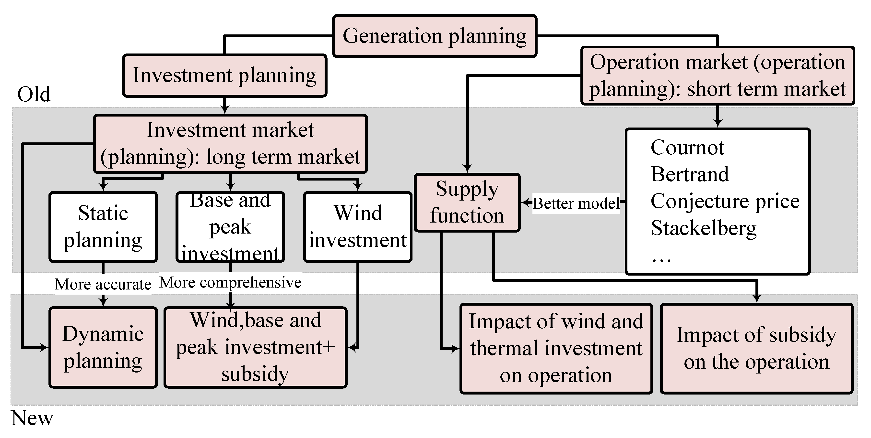
  • The model presents more reliable and better results if those that are intended for the short-term market include the market clearing aspect, whereas those intended for the longer term take into account investment. Therefore, the investment problem in this paper is bi-level; however, those presented in [5,18,19,20,21,22,23,24] are not bi-level.
  • In those models that have been proposed for market clearing, the supply function model in particular is a more accurate and realistic model when compared to others. Therefore, in this respect, a supply function model is used in the spot market whilst Refs. [25,26,27,28,29] make use of other models;
  • In this paper, three different load range technologies, including base, peak and wind plant are considered as the candidate units for investment and each technology has different options for investment capacity. However, candidate units for investment in [5,21,25,27,30] are wind unit and in [14,19,20,22,26,31,32,33,34,35,36,37,38,39] are other technologies. In addition, in this paper, the subsidy is considered in order to stimulate investment in the wind unit. This approach is more in line with reality, whilst largely overlooked in previous cases;
  • The proposed model is a dynamic one, whilst the dynamic nature of investment decisions has not been considered in papers concerning wind energy [3,25,40,41] and other technologies [19,20,22,26,32,34,35,36,37,38,39]. Therefore, the multi-period stochastic model consisting of transmission network constraints is presented here;
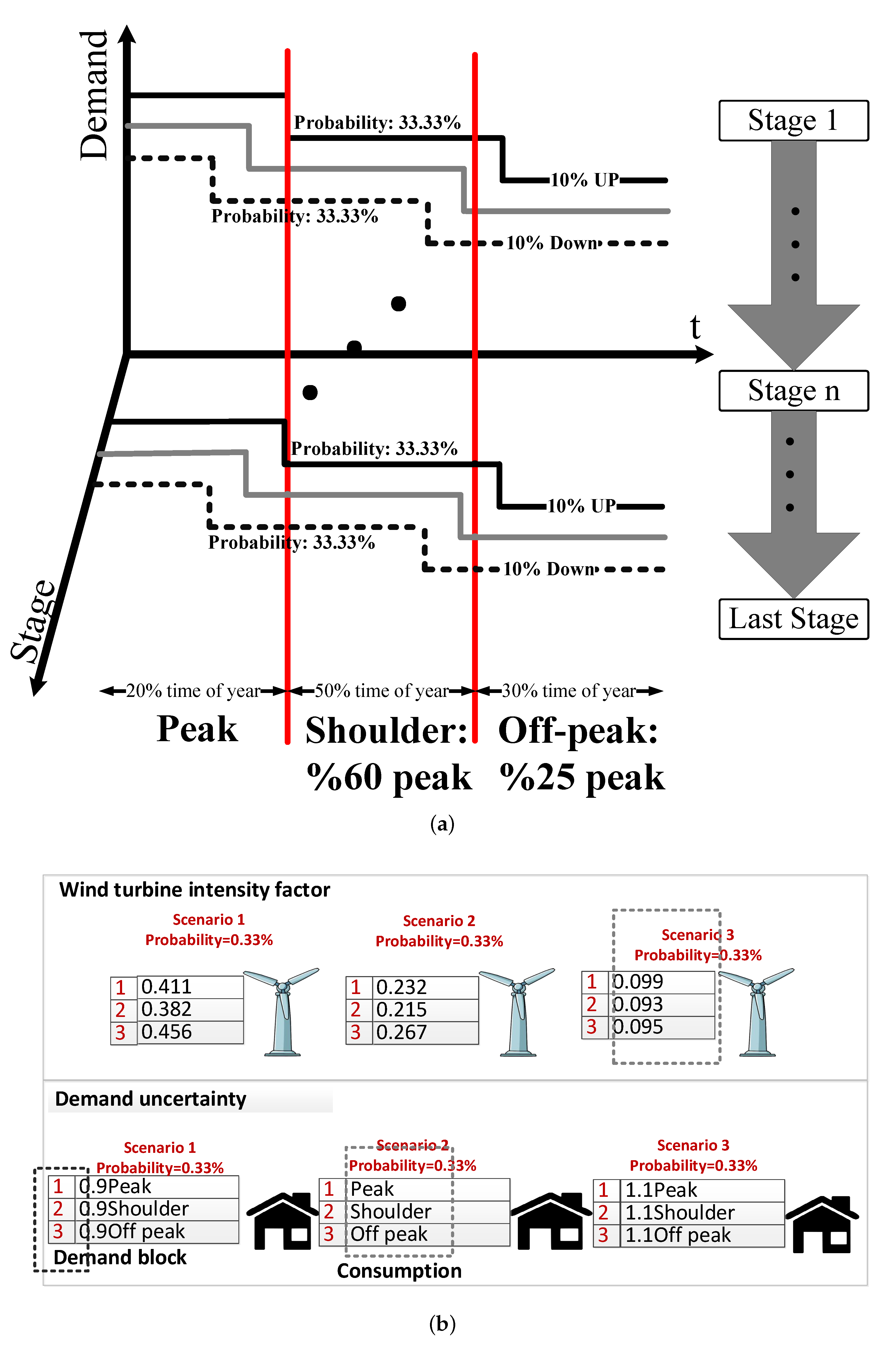
  • In this network, consideration is given to the uncertainty in the generation of electricity from wind power along with demand consumption. These uncertainties are modeled by means of a scenario based approach.
  • In addition, conventional producers are assumed to be competitive, i.e., they offer their respective productions at their marginal costs.
Considering the context above, contributions of this paper are as following:
  • to propose a wind investment model considering different load ranges of power plants so that the best production technology in the optimized location are offered.
  • to envelope a wind investment multi-stage model for sustainable electricity energy markets
  • to provide a methodology to investigate subsidies in both planning and operating planning in a network-constrained electricity market as a game-theoretic model.
  • To implement the proposed model to Mazandaran Regional Electric Company (MREC) as a real power network and comprehensively analyze the related results.

2. Planning Features

Dynamic multi-stage property: Planning in this article is done for 10 stages. Each stage can include one to several years depending on the terms planner. The annual discount rate of each stage in the dynamic approach is assumed to be 8.7%. Non-anticipativity issues should be analyzed according to the uncertainty of the demands and wind turbine production, as shown in Figure 2, combined with the dynamic approach of GEP.
Demand model property: the demand blocks are obtained from a stepwise approximation of the load-duration curve, as illustrated in Figure 2a. It is assumed that the per-stage demand is specified with three different demand blocks; namely peak, shoulder and off-peak. Annual growth of demands is assumed to be 6.2%. The weighting factors associated with each demand block (peak, shoulder and off-peak) are assumed to be 20%, 50% and 30%, respectively. In each year of the planning period, the weighting factor of the off-peak and shoulder blocks are considered to be 25% and 60% respectively of the associated forecasted peak demand. For the sake of simplicity, each demand considers one bid per block. For MREC demand, three uncertainties are considered, having the same probabilities as those shown in Figure 2b.
Investment technologies property: In this paper, three different load ranges of power plants including base, peak and wind units are considered for investment. Base technologies have relatively low operation costs but high investment costs due to supplying grid demand during all hours of the day. However, peak technologies, whilst also having low operation costs with high investment costs, only supply the grid during hours of peak demand.
In this article, it is assumed that the grid includes the construction of wind turbines. Construction of these units involves higher investment costs than the peak and base units; however, it is assumed that the operation cost of wind turbines units is zero. Renewable energy such as wind resources are usually characterized by uncertainty. The uncertainty of wind turbines can be modeled using a set of scenarios. To represent the uncertainty related to wind production, only three wind intensity factors are considered, despite the fact that a larger number of scenarios may easily be considered for a typical wind turbine in this model. Limiting the number of intensity factors prevents an increase in the computational complexity and corresponding time to solve the mathematical model by means of software simulation. Therefore, nine uncertainties are obtained with respect to three uncertainties of demand.
The modeling of wind turbine and converter: the Kinetic energy produced by wind is converted into mechanical power by the wind turbine rotor:
P w t = 0.5 ρ π R 2 V 3 = 0.5 ρ π R 2 ( R λ ) 3 ( W R ) 3 ,
λ = W R R V ,
P m e c = C p ( λ , β ) P w t = 0.5 C P ( λ , β ) ρ π R 2 ( R λ ) 3 ( W R ) 3 .
Equations (1)–(3) present equations of wind turbine modelling. Equation (1) presents the output power for wind turbine so that ρ and R are the air density (kg/m 3 ) and the blade radius (m) accordingly. In addition, V, W R as well as λ present the wind speed (m/s), rotor speed (rad/s) and the turbine tip-speed ratio, respectively [42]. The relation between turbine mechanical power ( P m e c ) and available power ( P w t ) is represented by Equation (3) while C P and β are power coefficient and pitch angle, respectively.
Non-anticipativity property: it should be noted that there is an issue of non-anticipativity nature in the problem of stochastic multi-stage modelling [43]. Figure 3 shows the different states relating to this issue. If the scenarios considered in the model are independent and different from one another at all stages, these provisions should not be applied to the programming (Mode 1, Figure 3). The multi-stage problems that include uncertainty have two modes, if uncertainties in the scenarios being considered are the same in the process of multi-stage models. The constraints related to non-anticipativity properties should be applied to the model (Mode 3, Figure 3) if the problem of stochastic multi-stage is solved by optimization algorithms, such as heuristic algorithms, in order that each iteration results in a different optimal solution. In addition, applying non-anticipativity constraints to the program is optional, if GAMS solvers such as MILP, LP, and NLP are used that result in the same optimal solution in repeated results (iterations). As a result of these issues around optimization, the same result in the optimal solution is obtained for scenarios that are similar in some of the steps (Mode 2, Figure 3). Therefore, applying the non-anticipativity conditions to the program tends to increase the complexity of the model and the corresponding calculations’ volume; however, it has no effect on providing the optimal solution. This issue should be considered in the simulation results only to ensure the correct program process; it can be ignored in a model for simplifying purposes and to achieve less computation and complexity. In this article, the provisions of the non-anticipitivity properties can be omitted due to the fact that the defined scenarios are independent of each other and they do not have any similarities with cases spanning a 10-year planning period.
The aforementioned is similar to Mode 1 from Figure 3. For example, the dynamic stochastic [20,44] is similar to the work of this paper and case 1 of Figure 3 and the expressed model in [20] is similar to Mode 3 of Figure 3. The first-level variables, which correspond to the installed generation capacity of the investing agent, will not be stochastic variables, however, since a generation company can only make one investment decision due to the fact that it is impossible to know which scenario is going to occur in reality.

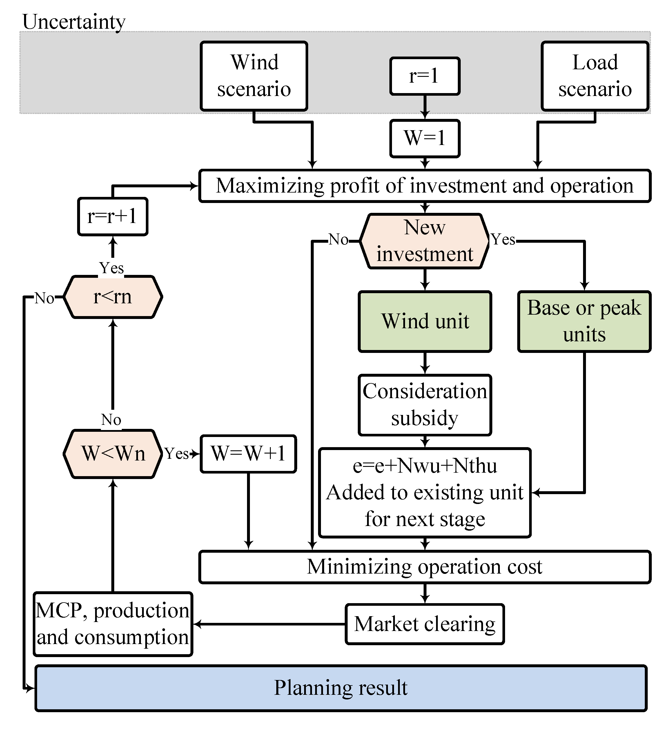
3. The Proposed Algorithm

This idea is solved by the algorithm presented in Figure 4. The planning carried out with the aim of maximizing the profits of the investment in the wind unit along with different load ranges, power plants including peak and base technologies, and investment in wind units that includes subsidies and grants to encourage investment is invested in the first year. New units are operated in subsequent years as existing units in the network. In the next stage, the intention is to minimize the operation cost so that the output at this stage is the market-clearing results, which includes market-clearing prices, unit production and consumption. This procedure is carried out for the next blocks in the first year. Overall, the benefits of investment and operation are maximized as a result of this planning. In Figure 4, N r , N w , N t , N wu and N thu are number of years, scenarios, time block, new wind units and new thermal units in the planning year, respectively. In addition, more information about bi-level modelling can be figured out in [19,43,44,45]. In addition, to perceive multi-stage planning, Ref. [14] is useful.

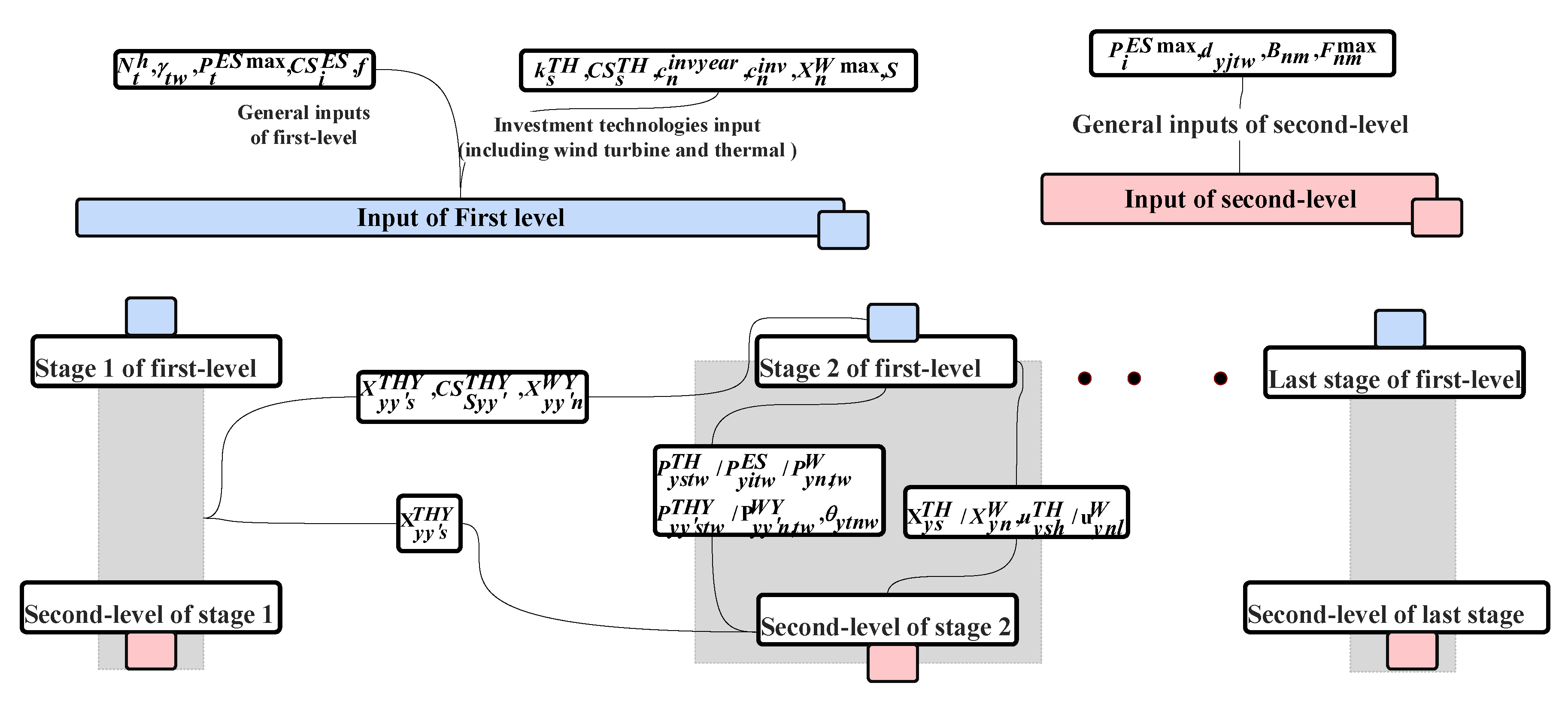
3.1. Inputs and Outputs

Figure 5 shows the input and output of each stage and stage to stage. The first-level includes 10 stages in which each stage includes a set of market-clearing issues for different scenarios and time demand blocks. The input of the first level for each stage includes input related to investment in different load ranges of power plants k s TH , CS s TH , c n invyear , c n inv , X n Wmax , S and the general input N t h , γ tw , P i ESmax , CS i ES , f.
First-level variables include X ys TH / X yn W , u ysh TH / u ynl W , and these have a certain effect in the second-level and are therefore considered to be second-level inputs. In addition, the second level includes the general inputs P i ESmax , d yjtw , B n m , and F nm max . The output of the second-level are variables P ystw TH / P yitw Es / P yn , tw W , P yy stw THY / P yy n , tw THY / P yy n , tw WY , and θ ytnw . These variables are also the variables of first-level. First-level input of each stage to the next stage includes variables P i Esmax , d yjtw , B nm , F nm max and the second-level input of the previous stage includes variables G ¯ theu .

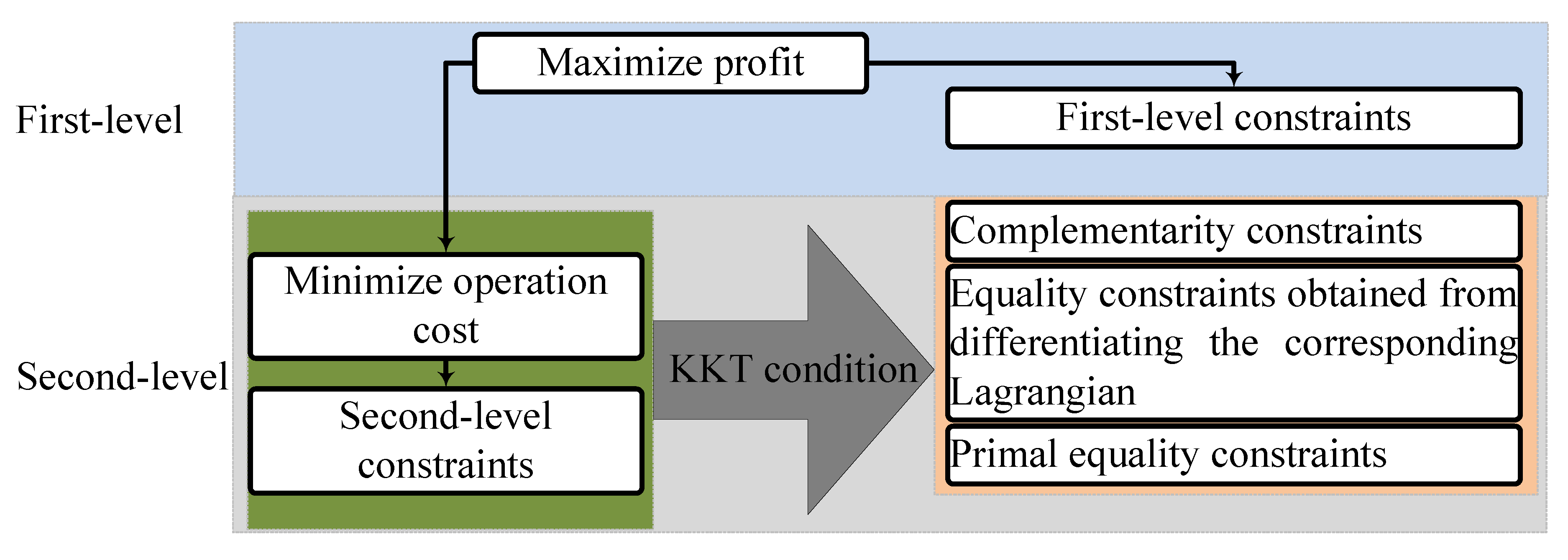
3.2. Converting Two Level Model to One Level Model

The market and the proposed algorithm are expressed using the bi-level model to implement the proposed ideas in this article. This bi-level model can be solved by heuristic algorithms, GAMS solvers and so forth. The GAMS solvers are used to solve the model proposed in this paper. For this purpose, the bi-level model is converted to a one-level problem and then the optimal solution is obtained using the available solvers, as shown in Figure 6. The second-level problem has constraints including DC power flow, limitations of unit production, and balance between production and consumption. Therefore, the second-level problem is a linear problem and therefore convex. Thus, karush kuhn tucker (KKT) conditions can be used to convert the bi-level problem into a one-level problem. Furthermore, complimentary constraints obtained from KKT conditions are linear when using the theory of big M. The resulting mathematical model becomes a problem of MILP after linearization of the nonlinear relationships and therefore it is solvable by MILP solvers in GAMS.

4. Mathematical Formulation

In the following sub-sections, the mathematical formulation of this paper is presented. In order to introduce the model, we define the following sets, parameters and decision variables.

4.1. The Bi-Level Model

The first-level represents the investment problem of the conventional producers who are seeking to maximize the present value of the total profit of investment (whether base or peak) and of operation. Due to the dynamic nature of the planning problem, dynamic dependency constraints exist in the first-level. The second-level problem represents the market-clearing. The clearing of the market for any given operating condition is represented as an optimization problem that identifies the operating decisions that maximize social welfare. In this model, maximizing the social welfare is equivalent to minimizing the generation cost. The market clearing problem is constrained by the DC power flow equations, transmission network limitations and units’ capacity limits. The output of the second-level problem is nodal prices (dual variables associated with the power balance constraints), which are fed back to the first-level.
The multi-period stochastic investment problem is formulated using the following bi-level model, which comprises the first-level problem, i.e., Equations (4)–(12), and a collection of second-level problems, i.e., Equations (14)–(20).
First level: The objective function (i.e., Equation (4)) is the present value of the projected profit (expected revenue offset by investment cost) in the planning horizon, which comprises three terms. The first and second terms of profit function (i.e., Equation (4)) are associated with the investment cost of new units, including peak and base technologies and wind units, respectively. The third term of the profit function (i.e., Equation (4)) is the expected profit obtained by selling energy in the spot market. Equation (5) states that investment options for new base or peak units are only available in discrete blocks, just as that of wind investment modelled through Equation (6). These equations impose the constraint that only one technology is binding and determines the new technology to be installed at each bus of the system. It should be noted that, based on Equations (5) and (6), the producer can either open exactly one new plant each year, or choose one option for installing it. These constraints define the maximum capacity of wind units along a multi-stage horizon that can be constructed in each location with wind power facilities. The dynamic dependency constraints on the base or peak investment decision variables are represented in Equations (7) and (8), while Equation (9) is related to the dynamic dependency constraints applicable to the wind investment. The new units are operated in the next years as existing units in the network (Equations (7) and (9)). Equation (8) is related to the marginal cost of a new base or peak units in subsequent years. Equation (10) enforces that wind generation at each bus scenario is limited to the installed wind power at the corresponding bus multiplied by a factor that models the wind intensity at that bus and scenario. Equation (11) as the dynamic dependency constraint shows wind production constraints in the years after the establishment of new units. The available budget limitation is represented in Equation (12) for investment in wind and new thermal units.
Second level: The market clearing problems are represented by the negative social welfare expressed Equations (13)–(20). Equation (14) represents the energy balance at each bus, this being the associated dual variables’ LMPs or nodal prices. Equations (15)–(19) impose power bounds for blocks of generation constraints, power flow and angle bounds. Equation (20) fixes the voltage angle at the reference bus. Dual variables are indicated at the relevant constraints following a colon:
First level objective function:
min y ( 1 1 + y ) y X s TH k s TH + y ( 1 1 + f ) y t ( 1 S ) c n inv X n W y ( 1 1 + f ) y t N t h w γ tw n P n , tw W λ n , tw + n y P yy n , tw WY λ n , tw + s P ystw TH λ n , tw s P ys , tw TH CS TH + s y P yy stw THY λ n , tw s y P yy stw THY CS Syy THY + i P yitw ES i P yitw ES CS i ES .
First level subjected to:
Subject to:
X ys TH = h u ysh TH X ysh TH , h u ysh TH = 1 u ysh TH { 0 , 1 } : y , s , h ,
X yn W = L u ynl W X nl W , L u ynl W = 1 u ynl W { 0 , 1 } : y , l , n ,
X yy s THY = X ys TH , y , y { X yy TH > 0 , y > y } , s ,
CS syy THY = CS s TH , y , y { X yy TH > 0 , y > y } , s ,
X yy n WY = X yn W , y , y { X y n W > 0 , y > y } , n ,
P yn , tw W K n , tw X yn W : y , n , t , w ,
0 P yy n , tw WY X yy n WY , y , y { X y n W > 0 , y > y } , t , n , w ,
y ( 1 1 + f ) y ( n ( 1 S ) C n inv X n W + k s TH X ys TH k max ) .
Second level objective function:
min i P yitw ES CS i ES + s P yStw TH CS S TH + s P yy stw THY CS S y THY , y , t , w .
Second level subjected to:
i P yitw ES + s P ystw TH + P yy n , tw WY + P yy stw THY + P yntw W m B nm P . U S b ( θ ytnw θ ytmw ) = j d yitw : λ ntw n , t , y , w ,
0 P yitw ES P yi ESmax : ϕ yitw min , ϕ yitw max y , i , t , w ,
0 P ystw TH X ys TH : μ ystw min , μ ystw max : y , s , t , w ,
0 P yy stw THY X yy s THY : μ yy stw THYmin , μ yy stw THYmax y , y { X y s TH > 0 , y > y } , t , s , w ,
F nm max B nm P . U s b ( θ ytnw θ ytmw ) F nm max : v ytnmw min , v ytnmw max n , m , t , y , w ,
π θ ytnw π : ζ ytnw min , ζ ytnw max , n , t , y , w ,
θ ytnw = 0 : ζ ytw 1 n = 1 , t , y , w .

MPEC

The bi-level problem (i.e., Equations (4)–(20)) can be converted to a single level problem (MPEC) by enforcing KKT conditions to the second-level problems [14,20,27]. These are represented by Equations (21)–(35). This transformation is possible because the lower-level problems are continuous and linear (and thus convex). The resulting problem is an MPEC, which includes nonlinearities in the objective function and in the complementarity conditions. These nonlinearities could be transformed into equivalent linear terms. Using this linearization, the investment problem can be finally expressed by the following MILP problem, as presented in the algorithm in Figure 4. To find a linear expression for n Ω N P n , tw W λ n , tw + s P ystw TH λ n , tw + i P yitw ES λ n , tw + s y P yy stw THY λ n , tw in Equation (4), we use the strong duality theorem and some of the KKT equalities [31]. The strong duality theorem says that, if a problem is convex, the objective functions of the primal and dual problems have the same value at the optimum.
Objective function of MPEC:
min y ( 1 1 + f ) y k s TH X ys TH + y ( 1 1 + f ) y t ( 1 S ) C n inv X yn W y ( 1 1 + f ) y t N t h w γ tw λ yn , tw d yj , tw i Ω N ϕ yitw max n V ytnw min F nm max n V ytnw max F nm max n ( ζ ytnw min + ζ ytnw max ) π i P yitw Es CS i ES s P ystw TH CS s TH s y P yy stw THY CS Syy THY .
MPEC subjected to:
  • First-level constraints: Equations (5)–(12).
  • Primal equality constraints equal to second-level: Equations (14)–(20).
  • Equality constraints obtained from differentiating the corresponding Lagrangian:
    CS i ES λ yntw + ϕ yitw max ϕ yitw min = 0 : y , i ,
    CS s TH λ yntw + μ ystw max μ ystw min = 0 : y , s ,
    CS s y y THY λ yntw + μ yy stw THYmax μ yy stw THYmin = 0 : y , s ,
    m B nm P . U S b ( λ ytnw λ ytmw ) + m B nm P . U S b ( V ytnmw max V ytmnw max ) + m B nm P . U S b ( V ytnmw min V ytmnw min ) + ζ ytnw max ζ ytnw min .
  • Complimentary constraints by KKT:
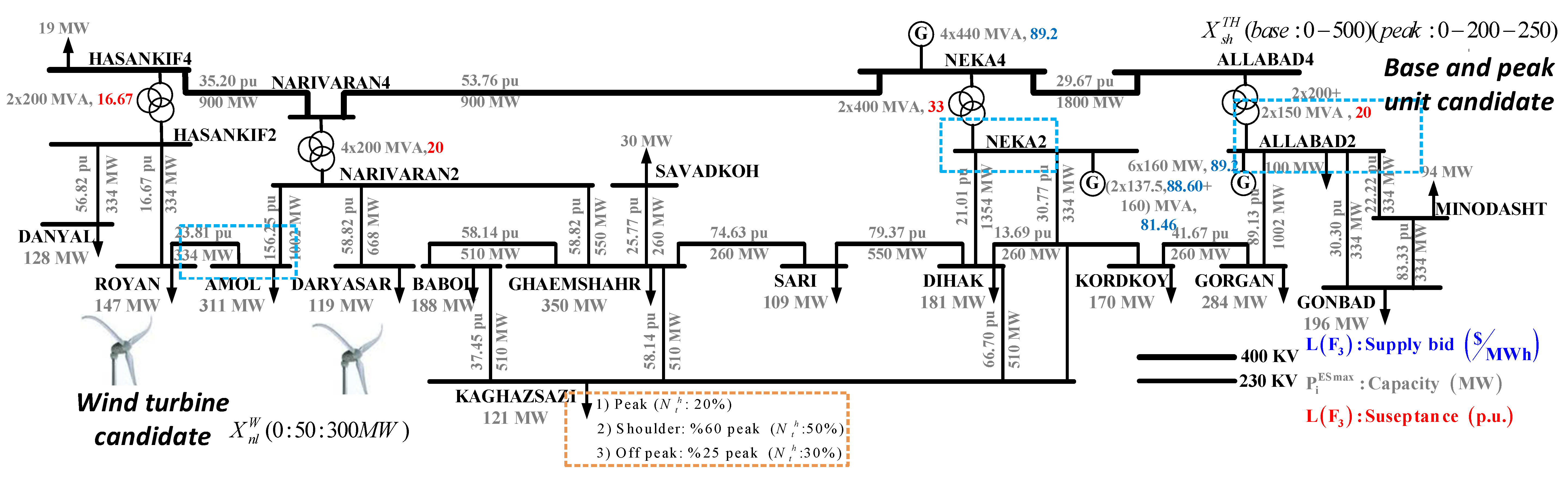
    0 P ystw TH μ ystw min 0 y , t , i , w ,
    0 P yitw EX ϕ itw min 0 y , i , t , w ,
    0 ( X ys TH P ystw TH ) μ ystw max 0 y , s , t , w ,
    0 P yy stw THY μ yy stw THYmin y , s , t , w ,
    0 ( X yy s THY P yy stw THY ) μ yy stw THYmax y , s , t , w ,
    0 ( P i EXmax P yitw EX ) ϕ itw max 0 y , i , t , w ,
    0 [ F nm max B nm P . U + S b ( θ ytnw θ ytmw ) ] V ytnmw max 0 y , t , n , m , w ,
    0 [ F nm max + B nm P . U + S b ( θ ytnw θ ytmw ) ] V ytnmw min 0 y , t , n , m , w ,
    0 ( π θ ytnw ) ζ ytnw max 0 y , t , n , w ,
    0 ( π + θ ytnw ) ζ ytnw min 0 y , t , n , w .
Equations (26)–(35) are linearized as follows [14,27]:
The complementarity condition
0 a b 0
can be replaced by
a 0 , b 0 , a τ M , b ( 1 τ ) M , τ { 0 , 1 } ,
where M is a large enough constant.

5. Case Studies

In this section, the efficiency of the proposed framework is examined through a real case study. The case study is the MAZANDARAN regional electric company (MREC) transmission network as a section of an IRAN interconnected power system.

Case Study: MREC Network
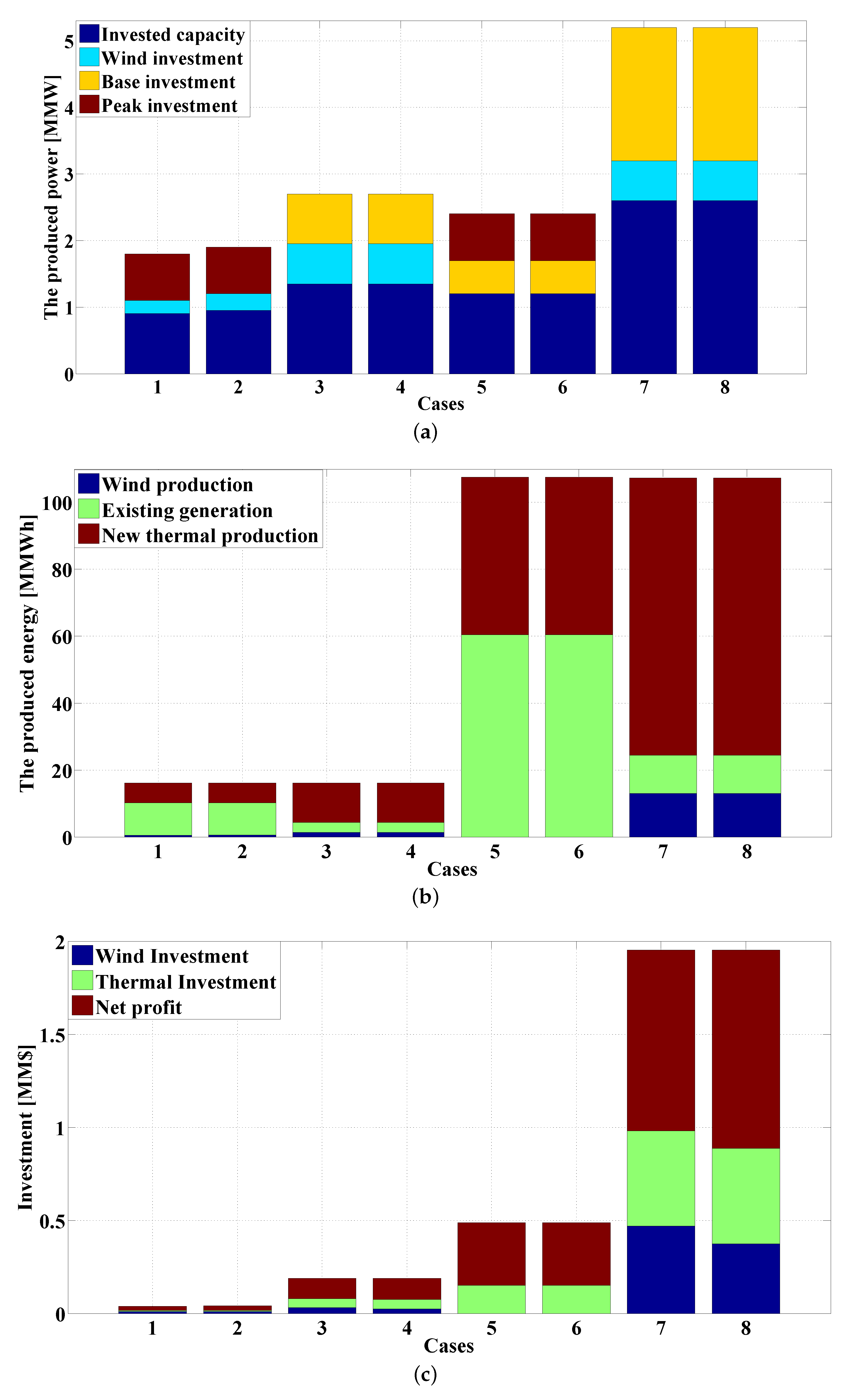
A single-line diagram representing the MREC transmission network is shown in Figure 7 [14,46]. The candidate buses for construction of the new base and peak units are assumed to be AMOL, ALIABAD and NEKA, all of which operate at 230 kV. In addition, buses ROYAN and DARYASAR are considered as candidate sites for construction of the new wind units. The maximum wind capacity that can be installed at these buses is equal to 300 MW for each bus.
The cases considered for the MREC transmission network are characterized in Table 1. The second column of this table gives the type of planning (static or dynamic) and columns 3 and 4 identify the subsidy percentage and the available budget, respectively. In Cases 1–4, the type of planning is static, while Cases 5–8 refer to dynamic cases. In addition, in Cases 2, 4, 6 and 8, consideration has been made of the impact of subsidy on the wind investment. In these cases, the subsidy percentage is assumed to be 20%. The proposed model is solved using Solver XPRESS software GAMS (IBM ILOG CPLEX Solver, 11.0.1, Armonk, NY, USA) [47].
Case #1 
total thermal investment is equal to 700 MW in the peak technology due to budget limitations and offset by their investment cost with respect to base technology. In this case, the total capacity added by the producer in the planning horizon has been established at 900 MW, resulting in the producer investing 200 MW in the wind technology and 700 MW in the peak technology. In this case, total thermal investment is attributable to peak technology due to budget limitation and less their investment cost with respect to base technology. The existing units supply 9.78 MMWh of the energy consumed by the network and thereby play an important role in the provision of energy to the MREC network;
Case #2 
Investment in wind units in this case is increased by 50 MW compared with Case #1 due to a 20% subsidy. In addition, the investment cost of wind units is the same as Case #1. In this case, the production of wind units has increased by 25.58%. Therefore, the net profit in Case #2 has increased by 18.44% with respect to Case #1;
Case #3 
The total capacity added by the producer in Case #3 has increased by 450 MW compared with Case #1 by increasing the budget from 15 M$ to 150 M$. Investment in wind units in this case has increased by 400 MW compared with the Case #1 due to an increase in the budget. In addition, the total thermal investment is base technology so that 750 MW is added to the MREC network. In Case #3, the production of wind and new thermal units have been increased by 201.62% and 98.15% compared with Case #1, respectively. In addition, the net profit in the planning horizon has been obtained equal to 108 M$ that it has been increased by 389.35% with respect to Case #1;
Case #4 
In Case #4, investment in wind and thermal units is the same as Case #3. In this case, subsidy has no effect on wind investment because the total capacity of wind units added to network is the same as in Case #3. In addition, the production of different units is the same as Case #3. However, the investment cost of wind units has decreased by 20% due to the 20% subsidy. As a result, the investor’s net profit has increased by 5.56% compared with Case #3;
Case #5 
In this case, the total capacity added by the producer in the planning duration has been determined to be 1200 MW, resulting in the producer investing 500 MW in the base technology and 700 MW in the peak technology, while no wind unit was constructed in the MREC network. This is the result of the desire to invest in units that have a lower investment cost due to the budget limitations. In addition, distribution of the investment are as follows: 200 MW on peak technology in the first year, 500 MW on base technology in the fifth year, 250 MW on peak technology in the eighth year and 250 MW on peak technology in the ninth and tenth years. Due to lack of generation in the western region, the total capacity has been constructed in AMOL located in this region.
Case #6 
All output of Case #6 is the same as Case #5; consequently, the consideration of a 20% subsidy has no influence on the desire to invest in wind units. It can be observed that the 20% subsidy is not enough to encourage investment in wind units and therefore the capacity of wind units is zero in this network.
Case #7 
In Case #3, the total capacity added by the investor has increased by 1400 MW compared with Case #5 and Investment in wind units in this case have been increased by 600 MW compared with the Case #1. In addition, total thermal investment is base technology so that 2000 MW base technologies are added to the MREC network. In Case #7, the production of new thermal units has been increased by 75.89% compared with Case #5, while the production of existing units decreased by 81.04%. In addition, the production of wind units has been increased from 0 MMWh to 12.97 MMWh with respect to Case #5. Thus, the total net profit in the planning duration is predicted to be 973.28 M$, an increase of 188.86% with respect to Case #5.
Case #8 
In this case, investment in wind and thermal units, and the production of different units, is the same as Case #7. However, investment cost of wind units has been decreased by 20% due to the 20% subsidy. As a result, the investor’s net profit has been increased by 9.62% compared with Case #3.
Figure 8 shows the result of GEP for MREC network for: (a) the produced power, (b) the produced energy, and (c) investment. Figure 9 depicts the percentages related to the budget, investment cost and total net profit for each case in the planning period. For example, the percentage related to the budget, investment cost and total net profit in the Case #1 are shown to be equal 29%, 29% and 42%, respectively, corresponding to 15, 14.99 and 22.07 when expressed in M$. The net profit in Case #5 and Case #6 in the dynamic approach has been increased by 26.19% and 12.77% compared to Case #1 and Case #2 in the static approach, respectively. Furthermore, the investment cost has been decreased by 17.24% and 11.11%, respectively. In addition, the net profit in Case #3 and Case #4 in the static approach has been increased by 14.28% and 9.68% compared to Case #7 and Case #8 in the dynamic approach, respectively. Furthermore, the investment cost has been decreased by 14.28% and 12%, respectively. Therefore, it can be seen that the percentage profit as a result of increasing the available budget for both static and dynamic planning. For lower budgets, the percentage profit yielded by the dynamic approach exceeds that of the static approach so that the investment cost in the former is less than in the latter. However, if a larger budget is available, the percentage profit yielded by the static approach exceeds that of the dynamic approach, whilst the former requires a lower investment. The use of a subsidy can increase investor profit if it stimulates investment in wind technologies. In addition, the investment cost decreases in these cases. It can be seen that the degree of investment increases when the dynamic approach is applied, when compared to the static approach. Moreover, consideration of the dynamic versus static trade-offs when the planning of generation capacity leads to accurate and realistic results in the expansion planning.

6. Conclusions

This paper has presented a model for the expansion planning of wind resources in power systems at a multi-stage horizon. In this paper, the power system consists of a combination of fossil fuel technologies and wind resources for investment. Real case studies were considered and analyzed. The features of the proposed model and simulation results led to following conclusions:
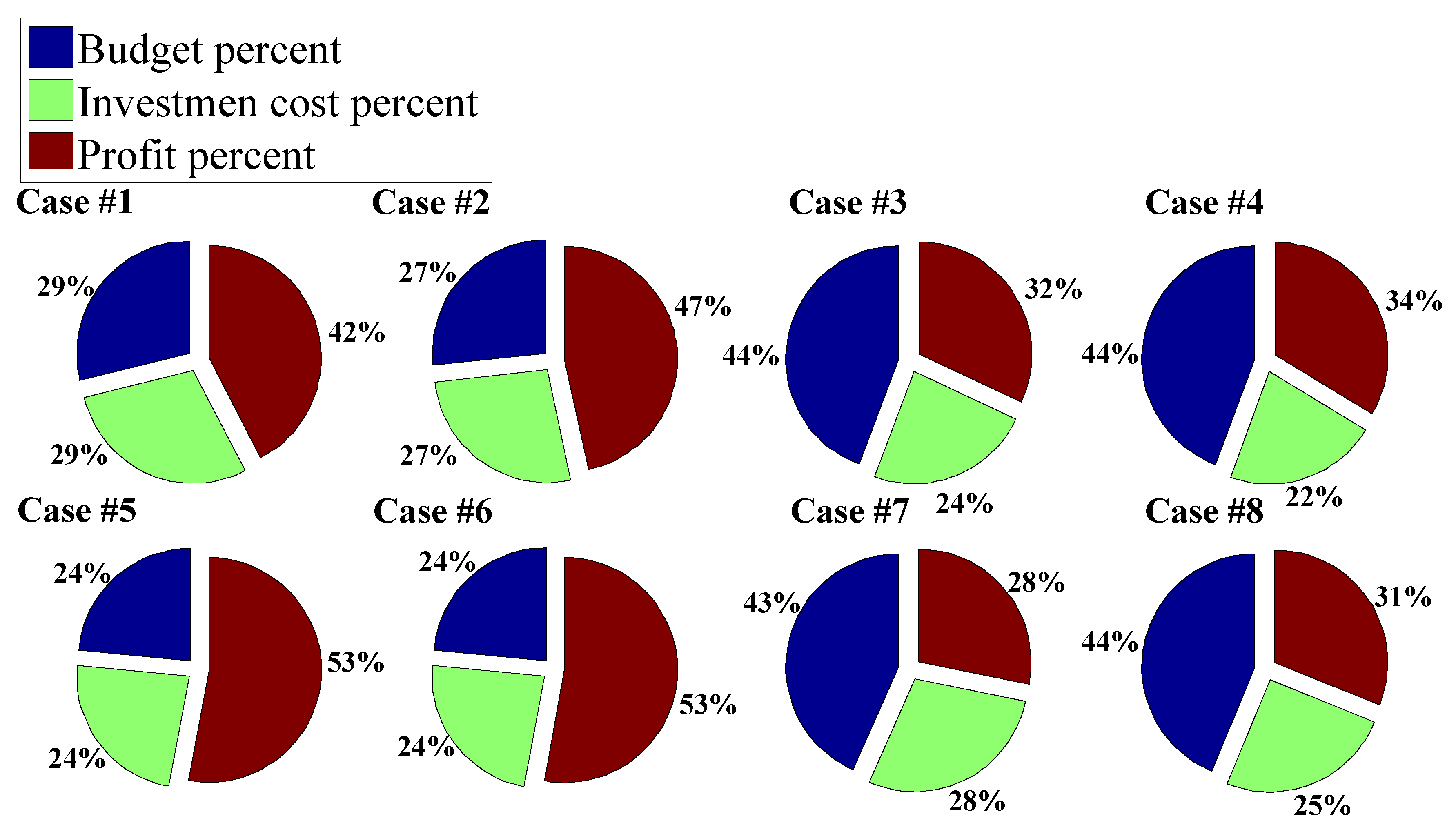
  • It can be seen that the percentage profit decreases as a result of increasing the available budget for both static and dynamic planning. At a lower budgetary level, the percentage profit yielded by the dynamic approach is more than that of the static approach so that the investment cost of the dynamic approach is less than the static. However, when the budgetary level is higher, the percentage profit in the static approach exceeds that of the dynamic approach while the static approach has a lower investment cost. The effect of a subsidy is to increase investor profit if the subsidy encourages investment on the wind technologies. In addition, the investment cost decreases in these cases. It can be seen that the total investor contribution has been increased in the dynamic approach with respect to the static one. Moreover, using the dynamic versus static approach in the planning of generation capacity leads to accurate and realistic results in the expansion planning.
  • Additional work is underway to represent the strategic behaviour of market participants other than wind and new thermal producers. The proposed model can be adapted to consider the impact of transmission expansion plans, availability of gas transmission networks, tax policy, DSM plans and uncertainty in the demand growth.

Author Contributions

All authors contributed equally to this work and all authors have read and approved the final manuscript.

Funding

This research received no external funding.

Conflicts of Interest

The authors declare no conflict of interest.

Nomenclature

Indices
windex for scenario
y/y indexes for stage (year)
tindex for demand blocks
s/i/jindexes for new base or peak units/existing generation unit and demand
h/linvestment capacity of new base or peak unit s/wind power at bus n (MW)
n/mindexes for bus
Acronyms
N t h weight of demand block t in year y
γ weight of scenario w in demand block t
k s TH / c n invyear annualized investment cost of base or peak units/wind power (€/MW)
c n inv investment cost of wind power at bus n
X n Wmax maximum wind capacity that can be installed at bus n
X sh Th / X nl W option h/l for investment capacity of new base or peak units s/wind power at bus n (MW)
P i ESmax capacity of existing generation unit i of strategic producer (MW)
d yjtw load of demand j in block t and year y (MW)
CS s TH / CS i ES price offered by new base or peak units/existing unit producer (€/MWh)
B nm susceptance of line n-m (p.u.)
F nm max transmission capacity of line n-m (MW)
fDiscount rate
SSubsidy percent
Decision variables
X ys TH / X yn W capacity investment of new unit s/wind power at bus n (MW)
u ysh TH / u ynl W binary variable that is equal to 1 if the h/lth investment option determines the base or peak unit/wind power is selected in year y
X yy s THY / X yy n WY available capacity of new unit s/wind power at bus n in year y’, in the years after the installation in year y (MW)
P ystw TH / P yitw ES / P yn , tw W power produced by new base or peak units s/existing unit i/wind power at bus n, in year y, demand block t and scenario w (MW)
P ystw TH / P yitw ES / P yn , tw W power produced by new base or peak units s/wind power at bus n, in year y’, in the years after the installation in year y (MW)
CS Syy THY price offered by new base or peak units producer a, in year y’, In the years after the installation in year y (€/MWh)
θ ytnw voltage angle of bus n, in year y, demand block t and scenario w

References

  1. Bagheri, A.; Monsef, H.; Lesani, H. Renewable power generation employed in an integrated dynamic distribution network expansion planning. Electr. Power Syst. Res. 2015, 127, 280–296. [Google Scholar] [CrossRef]
  2. Kahraman, C.; Onar, S.C.; Oztaysi, B. A Comparison of Wind Energy Investment Alternatives Using Interval-Valued Intuitionistic Fuzzy Benefit/Cost Analysis. Sustainability 2016, 8, 118. [Google Scholar] [CrossRef]
  3. Lumbreras, S.; Ramos, A.; Banez-Chicharro, F. Optimal transmission network expansion planning in real-sized power systems with high renewable penetration. Electr. Power Syst. Res. 2017, 149, 76–88. [Google Scholar] [CrossRef]
  4. Gan, L.; Li, G.; Zhou, M. Coordinated planning of large-scale wind farm integration system and regional transmission network considering static voltage stability constraints. Electr. Power Syst. Res. 2016, 136, 298–308. [Google Scholar] [CrossRef]
  5. Kamalinia, S.; Shahidehpour, M.; Khodaei, A. Security-constrained expansion planning of fast-response units for wind integration. Electr. Power Syst. Res. 2011, 81, 107–116. [Google Scholar] [CrossRef]
  6. You, S.; Hadley, S.W.; Shankar, M.; Liu, Y. Co-optimizing generation and transmission expansion with wind power in large-scale power grids—Implementation in the US Eastern Interconnection. Electr. Power Syst. Res. 2016, 133, 209–218. [Google Scholar] [CrossRef] [Green Version]
  7. Syed, I.M.; Raahemifar, K. Predictive energy management, control and communication system for grid tied wind energy conversion systems. Electr. Power Syst. Res. 2017, 142, 298–309. [Google Scholar] [CrossRef]
  8. Saboori, H.; Hemmati, R. Considering Carbon Capture and Storage in Electricity Generation Expansion Planning. IEEE Trans. Sustain. Energy 2016, 7, 1371–1378. [Google Scholar] [CrossRef]
  9. Nosair, H.; Bouffard, F. Flexibility Envelopes for Power System Operational Planning. IEEE Trans. Sustain. Energy 2015, 6, 800–809. [Google Scholar] [CrossRef]
  10. Valinejad, J.; Marzband, M.; Busawona, K.; Kyyrä, J.; Pouresmaeil, E. Investigating Wind Generation Investment Indices in Multi-Stage Planning. In Proceedings of the 5th International Symposium on Environment Friendly Energies and Applications (EFEA), Rome, Italy, 24–26 September 2018. [Google Scholar]
  11. Marzband, M.; Azarinejadian, F.; Savaghebi, M.; Pouresmaeil, E.; Guerrero, J.M.; Lightbody, G. Smart transactive energy framework in grid-connected multiple home microgrids under independent and coalition operations. Renew. Energy 2018, 126, 95–106. [Google Scholar] [CrossRef]
  12. Tavakoli, M.; Shokridehaki, F.; Akorede, M.F.; Marzband, M.; Vechiu, I.; Pouresmaeil, E. CVaR-based energy management scheme for optimal resilience and operational cost in commercial building microgrids. Int. J. Electr. Power Energy Syst. 2018, 100, 1–9. [Google Scholar] [CrossRef]
  13. Momoh, J.; Mili, L. Economic Market Design and Planning for Electric Power Systems; Wiley-IEEE Press: New York, NY, USA, 2009. [Google Scholar]
  14. Valinejad, J.; Marzband, M.; Akorede, M.F.; Barforoshi, T.; Jovanović, M. Generation expansion planning in electricity market considering uncertainty in load demand and presence of strategic GENCOs. Electr. Power Syst. Res. 2017, 152, 92–104. [Google Scholar] [CrossRef]
  15. Marzband, M.; Fouladfar, M.H.; Akorede, M.F.; Lightbody, G.; Pouresmaeil, E. Framework for smart transactive energy in home-microgrids considering coalition formation and demand side management. Sustain. Cities Soc. 2018, 40, 136–154. [Google Scholar] [CrossRef]
  16. Marzband, M.; Javadi, M.; Pourmousavi, S.A.; Lightbody, G. An advanced retail electricity market for active distribution systems and home microgrid interoperability based on game theory. Electr. Power Syst. Res. 2018, 157, 187–199. [Google Scholar] [CrossRef]
  17. Olsen, D.; Byron, J.; DeShazo, G.; Shirmohammadi, D.; Wald, J. Collaborative Transmission Planning: California’s Renewable Energy Transmission Initiative. IEEE Trans. Sustain. Energy 2012, 3, 837–844. [Google Scholar] [CrossRef]
  18. Soroudi, A.; Rabiee, A.; Keane, A. Information gap decision theory approach to deal with wind power uncertainty in unit commitment. Electr. Power Syst. Res. 2017, 145, 137–148. [Google Scholar] [CrossRef]
  19. Baringo, L.; Conejo, A. Wind Power Investment: A Benders Decomposition Approach. IEEE Trans. Power Syst. 2012, 27, 433–441. [Google Scholar] [CrossRef]
  20. Xiong, P.; Singh, C. Optimal Planning of Storage in Power Systems Integrated With Wind Power Generation. IEEE Trans. Sustain. Energy 2016, 7, 232–240. [Google Scholar] [CrossRef]
  21. Sun, C.; Bie, Z.; Xie, M.; Jiang, J. Assessing wind curtailment under different wind capacity considering the possibilistic uncertainty of wind resources. Electr. Power Syst. Res. 2016, 132, 39–46. [Google Scholar] [CrossRef]
  22. Li, S.; Coit, D.W.; Felder, F. Stochastic optimization for electric power generation expansion planning with discrete climate change scenarios. Electr. Power Syst. Res. 2016, 140, 401–412. [Google Scholar] [CrossRef] [Green Version]
  23. Tavakoli, M.; Shokridehaki, F.; Mousa Marzband, R.G.; Pouresmaeil, E. A two stage hierarchical control approach for the optimal energy management in commercial building microgrids based on local wind power and PEVs. Sustain. Cities Soc. 2018, 41, 332–340. [Google Scholar] [CrossRef]
  24. Hinojosa, V.H.; Velásquez, J. Improving the mathematical formulation of security-constrained generation capacity expansion planning using power transmission distribution factors and line outage distribution factors. Electr. Power Syst. Res. 2016, 140, 391–400. [Google Scholar] [CrossRef]
  25. Valenzuela, J.; Wang, J. A probabilistic model for assessing the long-term economics of wind energy. Electr. Power Syst. Res. 2011, 81, 853–861. [Google Scholar] [CrossRef]
  26. Zhang, T.; Baldick, R.; Deetjen, T. Optimized generation capacity expansion using a further improved screening curve method. Electr. Power Syst. Res. 2015, 124, 47–54. [Google Scholar] [CrossRef]
  27. Pineda, S.; Morales, J.; Ding, Y.; Østergaard, J. Impact of equipment failures and wind correlation on generation expansion planning. Electr. Power Syst. Res. 2014, 116, 451–458. [Google Scholar] [CrossRef] [Green Version]
  28. Brandi, R.B.S.; Ramos, T.P.; David, P.A.M.S.; Dias, B.H.; Marcato, A.L.M. Maximizing hydro share in peak demand of power systems long-term operation planning. Electr. Power Syst. Res. 2016, 141, 264–271. [Google Scholar] [CrossRef]
  29. Jabr, R. Robust Transmission Network Expansion Planning With Uncertain Renewable Generation and Loads. IEEE Trans. Power Syst. 2013, 28, 4558–4567. [Google Scholar] [CrossRef]
  30. Munoz, F.D.; Mills, A.D. Endogenous Assessment of the Capacity Value of Solar PV in Generation Investment Planning Studies. IEEE Trans. Sustain. Energy 2015, 6, 1574–1585. [Google Scholar] [CrossRef]
  31. Valinejad, J.; Barforoushi, T. Generation expansion planning in electricity markets: A novel framework based on dynamic stochastic MPEC. Int. J. Electr. Power Energy Syst. 2015, 70, 108–117. [Google Scholar] [CrossRef]
  32. Baringo, L.; Conejo, A. Strategic Wind Power Investment. IEEE Trans. Power Syst. 2014, 29, 1250–1260. [Google Scholar] [CrossRef]
  33. Valinejad, J.; Marzband, M.; Barforoushi, T.; Kyyrä, J.; Pouresmaeil, E. Dynamic stochastic EPEC model for Competition of Dominant Producers in Generation Expansion Planning. In Proceedings of the 5th International Symposium on Environment Friendly Energies and Applications (EFEA), Rome, Italy, 24–26 September 2018. [Google Scholar]
  34. Kim, J.-Y.; Kim, K.S. Integrated Model of Economic Generation System Expansion Plan for the Stable Operation of a Power Plant and the Response of Future Electricity Power Demand. Sustainability 2018, 10, 2417. [Google Scholar] [CrossRef]
  35. Khaligh, V.; Buygi, M.O.; Anvari-Moghaddam, A.; Guerrero, J. A Multi-Attribute Expansion Planning Model for Integrated Gas–Electricity System. Energies 2018, 11, 2573. [Google Scholar] [CrossRef]
  36. Ko, W.; Park, J.K.; Kim, M.K.; Heo, J.H. A Multi-Energy System Expansion Planning Method Using a Linearized Load-Energy Curve: A Case Study in South Korea. Energies 2017, 10, 1663. [Google Scholar] [CrossRef]
  37. Hong, S.; Cheng, H.; Zeng, P. An N-k Analytic Method of Composite Generation and Transmission with Interval Load. Energies 2017, 10, 168. [Google Scholar] [CrossRef]
  38. Zhou, X.; Guo, C.; Wang, Y.; Li, W. Optimal Expansion Co-Planning of Reconfigurable Electricity and Natural Gas Distribution Systems Incorporating Energy Hubs. Energies 2017, 10, 124. [Google Scholar] [CrossRef]
  39. Li, R.; Ma, H.; Wang, F.; Wang, Y.; Liu, Y.; Li, Z. Game Optimization Theory and Application in Distribution System Expansion Planning, Including Distributed Generation. Energies 2013, 6, 1101–1124. [Google Scholar] [CrossRef] [Green Version]
  40. Meng, K.; Yang, H.; Dong, Z.Y.; Guo, W.; Wen, F.; Xu, Z. Flexible Operational Planning Framework Considering Multiple Wind Energy Forecasting Service Providers. IEEE Trans. Sustain. Energy 2016, 7, 708–717. [Google Scholar] [CrossRef]
  41. Flores-Quiroz, A.; Palma-Behnke, R.; Zakeri, G.; Moreno, R. A column generation approach for solving generation expansion planning problems with high renewable energy penetration. Electr. Power Syst. Res. 2016, 136, 232–241. [Google Scholar] [CrossRef]
  42. Duong, M.Q.; Grimaccia, F.; Leva, S.; Mussetta, M.; Le, K.H. Improving transient stability in a grid-connected squirrel-cage induction generator wind turbine system using a fuzzy logic controller. Energies 2015, 8, 6328–6349. [Google Scholar] [CrossRef] [Green Version]
  43. Conejo, A.J.; Carrión, M.; Morales, J.M. Decision Making under Uncertainty in Electricity Markets; Springer: Berlin/Heidelberg, Germany, 2010. [Google Scholar]
  44. Kazempour, S.; Conejo, A.; Ruiz, C. Strategic Generation Investment Using a Complementarity Approach. IEEE Trans. Power Syst. 2011, 26, 940–948. [Google Scholar] [CrossRef]
  45. Drud, A. CONOPT. Available online: https://ampl.com/products/solvers/solvers-we-sell/conopt/ (accessed on 31 July 2012).
  46. Valinejad, J.; Oladi, Z.; Barforoshi, T.; Parvania, M. Stochastic Unit Commitment in the Presence of Demand Response Program Under Uncertainties. IJE Trans. B Appl. 2017, 30, 1134–1143. [Google Scholar]
  47. Brooke, D.; Kendrick, A.; Meeraus, R.; Raman, R. GAMS: A User’s Guide; GAMS Development Corp.: Washington, DC, USA, 1998. [Google Scholar]
Figure 1. Block diagram illustrating the effectiveness of investment and planning.
Sustainability 10 03811 g001
Figure 2. Features of demand and wind turbine. (a) piecewise approximation of the load duration curve for the planning year at a particular bus; (b) the uncertainty of demand and wind turbine.
Sustainability 10 03811 g002
Figure 3. Three different cases for the non-anticipativity condition in a multi-stage stochastic problem.
Sustainability 10 03811 g003
Figure 4. The algorithm for solving the proposal idea.
Sustainability 10 03811 g004
Figure 5. Input and output of each stage and stage to stage.
Sustainability 10 03811 g005
Figure 6. Converting the bi-level problem into one-level problem.
Sustainability 10 03811 g006
Figure 7. Single-line diagram of the MAZANDARAN Regional Electric Company (MREC) transmission network.
Sustainability 10 03811 g007
Figure 8. The result of GEP for MREC network. (a) the produced power; (b) the produced energy; (c) investment.
Sustainability 10 03811 g008
Figure 9. The percent related to the budget, investment cost and total net profit for each case.
Sustainability 10 03811 g009
Table 1. The cases considered for the MREC transmission network.
CasesPlanningSubsidy (%)Budget (M$)
#1Static015.0
#2Static2015.0
#3Static0150
#4Static20150
#5Dynamic0150
#6Dynamic20150
#7Dynamic01500
#8Dynamic201500

