Multiple Urban Domestic Water Systems: Method for Simultaneously Stabilized Robust Control Decision

1
School of Management Science and Engineering & China Institute of Manufacturing Development, Nanjing University of Information Science & Technology, Nanjing 210044, China
2
Department of Mathematics and Computer Science, University of North Carolina at Pembroke, Pembroke, NC 28372, USA
*
Author to whom correspondence should be addressed.
Sustainability 2018, 10(11), 4092; https://0-doi-org.brum.beds.ac.uk/10.3390/su10114092
Submission received: 14 September 2018
/
Revised: 2 November 2018
/
Accepted: 5 November 2018
/
Published: 8 November 2018
(This article belongs to the Special Issue Transition from China-Made to China-Innovation
)
Abstract
:The distribution of water resources and the degree of economic development in different cities will result in different parameters for the supply and demand of domestic water in each city. In this paper, a simultaneous stabilization and robust control method is proposed for decision-making regarding multiple urban domestic water systems. The urban water demand is expressed as the product of the urban domestic water consumption population and per capita domestic water consumption. The fixed capital investment and labor input of the urban domestic water supply industry are used as control variables. Based on the Lyapunov stability theory and the linear matrix inequality method, multiple urban domestic water supply and demand systems can accomplish asymptotical stability through the coordinated input of investment and labor. For an empirical analysis, we take six cities—Nanjing, Wuxi, Nantong, Yangzhou, Xuzhou, and Lianyungang—in Jiangsu Province, China, to study the simultaneously stabilized coordinated control scheme. The simulation results show that the same control scheme simultaneously achieves the asymptotic stability of these urban domestic water supply and demand systems, and is robust when it comes to the variation of system parameters. This method is particularly suitable for a water resources administrative agency to make a unified decision-making arrangement for water supply input in different areas. It will help synchronize multiple urban domestic water managements and reduce the difficulty of control.
1. Introduction
In recent years, China’s urbanization rate has been continuously increasing. According to the “2017 China statistical yearbook” (National Bureau of Statistics of China [1]), the urbanization rate in China was 46.99% in 2008, 49.95% in 2010, 56.10% in 2015, and 57.35% in 2016. The latest data released by the National Bureau of Statistics of China in 2018 showed that in 2017, China’s urbanization rate was further rising to 58.52%, an increase of 1.17% points compared to that of the previous year.
According to the “China water resources bulletin” issued by the Ministry of Water Resources of China, the total water consumption in China was 556.6 billion m3 in 1997, 549.8 billion m3 in 2000, 602.2 billion m3 in 2010, and 604.02 billion m3 in 2016. Domestic water consumption was 52.5 billion m3 in 1997, 57.5 billion m3 in 2000, 76.58 billion m3 in 2010, and 82.16 billion m3 in 2016. The proportion of domestic water consumption out of total water consumption was 9.4% in 1997, 10.5% in 2000, 12.7% in 2010, and 13.6% in 2016. The urban domestic water consumption was 24.7 billion m3 in 1997, 28.4 billion m3 in 2000, 47.2 billion m3 in 2010, and 63.68 billion m3 in 2016. The proportion of urban domestic water consumption in domestic water consumption was 47% in 1997, 49.4% in 2000, 61.6% in 2010, and 77.5% in 2016.
According to the above statistics, with the fast growth of economic development and accelerated urbanization, China’s domestic water consumption and urban domestic water consumption are dramatically expanding. Moreover, the ratio of domestic water consumption to total water consumption and the ratio of urban domestic water consumption to domestic water consumption are both rising. The proportion of domestic water consumption to total water consumption was 9.4% in 1997, 10.5% in 2000, 12.7% in 2010, and 13.6% in 2016. The proportion of urban domestic water consumption to the total domestic water consumption was 47% in 1997, 49.4% in 2000, 61.6% in 2010, and 77.5% in 2016.
Safeguarding urban water supply security is of great significance for ensuring the basic needs of urban people for domestic water and maintaining the normal operation of the urban economy and the harmony and stability of society (Wang [2]). However, there are differences in levels of urban economic and social development and in geographical conditions, which require variable parameter values in domestic water supply and demand systems. For multiple urban domestic water systems with different parameters, if a unified control decision method can be used in domestic water inputs, the multiple urban domestic water systems can achieve asymptotic stability up to the balance between supply and demand, which will provide a useful reference for the synchronization of multiple urban domestic water management.
In water management, dynamic optimization and control decision-making methods have achieved some meaningful research results. In 2001, Mourad and Lachhab et al. studied the adaptive control method for controlling the water flow consumption through a pump for a discrete-time water supply system (Mourad and Lachhab et al. [3]). In 2001, Sahu and Gupta studied the dynamic programming method for deterministic systems of reservoir management (Sahu and Gupta [4]). In 2003, Eker and Grimble et al. studied the robust control method of application control for a water supply system consisting of a group of pumping stations (Eker and Grimble et al. [5]). In 2004, Roseta-Palma and Xepapadeas studied robust control methods in water management (Roseta-Palma and Xepapadeas [6]). In 2006, Fang and Wang studied the optimal control method for reservoir scheduling with state space constraints on water storage variables (Fang and Wang [7]). In 2010, Li and Chen studied the robust control method of investment decision-making for discrete-time urban supply and demand water systems (Li and Chen [8]). In 2010 and 2011, Li and Chen studied the optimal control method for dynamic investment decision-making of urban water supply and demand systems (Li and Chen [9], Li [10]). In 2015, Li studied the optimal control method for simultaneous decision-making of urban domestic water system investment and labor input (Li [11]). In 2016, Pereira and de la Peña et al. studied the robust periodic model predictive control method for the domestic water system network (Pereira and de la Peña et al. [12]). In 2016, Sarbu and Ostafe proposed an improved linear optimization model based on linear programming for the urban water supply network system (Sarbu and Ostafe [13]). In 2017, Qaderi and Babanezhad proposed an artificial neural network model for predicting the cost of underground drinking water remediation (Qaderi and Babanezhad [14]). In 2018, Nguyen and Stewart et al. provided infrastructure planners with a means to re-engineer traditional urban water management practices through smart metering and informatics (Nguyen and Stewart et al. [15]); Li and Ma et al. studied the robust control decision-making method when the two production factors of investment and labor were simultaneously input for the discrete-time urban domestic water system (Li and Ma et al. [16]).
Simultaneous stabilization is the problem of determining a single controller, which simultaneously stabilizes a finite collection of plants (Kohan-Sedgh and Khayatian et al. [17]). Simultaneous stabilization is also a hard open problem in linear systems theory (Gündeş and Nanjangud [18]). In 2004, using the linear matrix inequality (LMI) approach, Chen and Chang et al. researched the simultaneous static output feedback stabilization problem for a collection of discrete-time interval systems (Chen and Chang et al. [19]). In 2006, Al-Awami and Abdel-Magid et al. studied the use of robust unified power flow controller (UPFC)-based stabilizers to damp low frequency oscillations (Al-Awami and Abdel-Magid et al. [20]). In 2013, Gündeş and Nanjangud researched the simultaneous stabilization of a finite set of linear, time-invariant (LTI), multi-input multi-output (MIMO) plants using LTI output feedback controllers. (Gündeş and Nanjangud [18]). In 2015, Ryan developed globally asymptotically stabilizing feedback for the problem of stabilization through the feedback of finitely many oscillators via bilinear control action with a common scalar input (Ryan [21]). In 2015, Wang and Miao et al. proposed a smooth time-varying controller to simultaneously address the stabilization and tracking problems of nonholonomic mobile robots for most admissible reference trajectories without switching (Wang and Miao et al. [22]). In 2015, Kaneko addressed the simultaneous stabilization problem for two linear systems in the behavioral framework (Kaneko [23]). In 2016, Kohan-Sedgh and Khayatian et al. proposed two convex methods based on structured slack variable and dilated matrix inequalities with a simultaneous output feedback stabilizer for continuous-time linear systems (Kohan-Sedgh and Khayatian et al. [17]).
In brief, the above achievements show that many dynamic optimization and control decision-making methods have been applied to water management, including adaptive control, dynamic programming, optimal control, robust periodic model predictive control, linear programming, and artificial neural network, etc. However, the above results mainly focused on water management and optimization in a single region, and were less concerned with the simultaneous optimization and control of water resources in multiple regions. In contrast, this coordinated control study aims to reduce the complexity of water resource management in multiple regions.
Literature has shown that the simultaneously stabilized robust control decision is an important but difficult problem. Its current application mainly lies in engineering control, and its application in social systems includes behavior control. However, its application does not seem to extend to the economic control of the water supply system. Therefore, the value added with respect to existing methods for simultaneously stabilized robust control decisions is as follows. This paper attempts to extend the simultaneously stabilized robust control method, which is mainly used in engineering, to the economic control of water management. Engineering control in water management, e.g., pump flow control, is important. Beyond that, however, the water industry is still a typical capital-intensive industry (Baumann and Boland et al. [24]). Consequently, it is also valuable for the long-term development of the water industry to improve the utilization efficiency of capital and labor input. In this paper, a simultaneous stabilization and robust control method is proposed for decision-making regarding multiple urban domestic water systems. This method attempts to improve the efficiency of investment and labor input, and to reduce the complexity of the control scheme for multiple urban domestic water managements. At present, research in this field is not common.
The objectives of this methodology are as follows. For multiple urban water systems with the same model structure but different parameters, a unified control scheme of investment and labor input is proposed, which makes the system state value of each city tend to the target value.
The limits of this methodology are as follows. This method is easier to apply to engineering control with a relatively clear system structure and parameters. For socio-economic systems such as water management, due to the complexity and variability of the system structure and parameters, the practical application of this method will be subject to certain constraints.
The process to define the methodology is as follows. Firstly, each state equation of the system is transformed appropriately, and then combined into matrix equations. Secondly, for the combined matrix equations, the state feedback control decision method is used to adjust the system state. The key to this method is to determine a state feedback gain matrix . This is achieved using the Lyapunov stability theory and the linear matrix inequality method. Finally, is substituted into the state feedback control equation and implemented according to the control scheme to achieve the system objectives.
The contribution of this paper to urban water management is: Fixed capital investment and labor input are common production factors, and have an impact on the operation of urban domestic water systems. This paper takes them as control variables to study the method for simultaneously stabilized robust control decisions for multiple urban domestic water systems.
This will help with the synchronization of water management in multiple cities. This method is especially valuable for the following situations: reducing the difficulty of control; and achieving unified water supply decision-making for different cities under their corresponding jurisdiction.
This approach could be more effective for urban water supply management under the central management system, which is used in China. Under this management mode, the higher-level administrative agency can undertake the unified management of each region under its jurisdiction, and has decision-making power in the input of production factors.
The structure of this paper is as follows. Section 2 develops the decision model for simultaneously stabilized robust control for multiple urban domestic water systems. With the use of fixed capital investment and labor input as control decision variables, the system objective is to design a unified control decision method, rendering multiple urban domestic water supply and demand systems asymptotically stable. In Section 3, we present the decision-making method designed for simultaneously stabilized robust control for multiple urban domestic water systems, and the model is solved using the Lyapunov stability theory and the linear matrix inequality method. In Section 4, a simulation is provided to illustrate the design, where six cities in Jiangsu Province are selected. Section 5 further explores the robustness of the proposed decision scheme. Furthermore, in Section 5, the limitations of the design are studied. Finally, Section 6 compares the model in this paper with the existing models, in relation to the aspects of water demand function, applicable object range, and control decision method. Section 6 also provides a summary of the paper.
2. Control Decision Model for the Inputs of Multiple Urban Domestic Water Systems
Levels of economic and social development differ, as do the distribution of water resources and the difficulty of exploitation. This leads to the difference in the parameter values in different urban water supply and demand systems.
Let us suppose that there are different cities, and the state equation of the domestic water demand function for city can be written as (Baumann and Boland et al. [24])
where is the time unit, is the urban domestic water consumption population, and is the per capita domestic water consumption for city . This is a widely used method for predicting urban water demand. There are other factors that characterize demand, for example, the economic situation of the people. In general, the impact of economic conditions on water demand is reflected in the positive correlation between the per capita domestic water consumption and the level of economic development of city .
The technical specifications for the analysis of the supply and demand balance of water resources in the China’s water conservancy industry standard (SL 429-2008) recommends to use the per capita daily water consumption index to predict domestic water (Ministry of Water Resources of China [25]).
If the per capita daily domestic water consumption index is used in this paper directly, this means that the time unit of system control decision is daily control. However, for multiple urban domestic water supply input control decision systems, the one-day time setting would be too short. Water management can be divided into a short cycle or a medium-long cycle. Daily management is a short cycle method, and water flow may be the main control means in this method. Such management is very important. Moreover, there is also a category of medium-long cycle water management method, which may be conducted based on a quarterly or annual cycle. In this paper, the investment and labor inputs in domestic water management are studied. Compared with the short cycle management method, such problems may be more suitable for adopting the medium-long cycle management method.
In this study, the time unit of the control decision system is set to one year. Correspondingly, , the per capita annual domestic water consumption of city , stands for the per capita daily domestic water consumption multiplied by the average number of days per year, i.e., 365. Therefore, there is no essential difference between the per capita annual domestic water consumption and the per capita daily domestic water consumption. For daily water management, it is necessary to consider the daily fluctuation. However, for annual water management, the importance of daily fluctuation is relatively minor. By adding the average daily water consumption, the average annual water consumption is . Since the average daily water consumption eliminates the effect of daily fluctuations, the average annual water consumption does not take this effect into account. In fact, since the control decisions studied in this paper are annual rather than daily cycles, the impact on daily water consumption fluctuations is eliminated by averaging.
The data of per capita domestic water consumption quoted below convert the original per capita daily domestic water consumption data into per capita annual domestic water consumption data.
A study of 21 countries, including China, the UK and Brazil, etc., shows that there is a positive correlation between per capita domestic water consumption and the social development level. This indicates that with the development of society and economy, the per capita domestic water consumption increases accordingly. There are two exceptions, the United States and Columbia, and their per capita water consumption is much higher than that of countries with comparable economic conditions. This is determined by the more abundant water resources of the two countries (Xu and Wang et al. [26]).
According to the “2017 China statistical yearbook”, in 2016, urban per capita annual domestic water consumption was 63.2 m3 in Beijing, 41.6 m3 in Tianjin, 37.8 m3 in Inner Mongolia (all located in northern China), 73.3 m3 in Shanghai, 78.6 m3 in Jiangsu (east), 89.8 m3 in Guangdong, 93.6 m3 in Guangxi (south), 55.3 m3 in Chongqing, 78.3 m3 in Sichuan (southwest), 58.1 m3 in Shaanxi, and 45.7 m3 in Gansu (northwest) (National Bureau of Statistics of China [1]).
According to Cui [27], statistics on water consumption in large cities with a population of over one million in China show that compared to northern cities, southern cities have more abundant water resources and higher per capita domestic water consumption. In 2002, the per capita annual domestic water consumption in northern cities was 79.0 m3, while that in southern cities was 123.8 m3. In the southern cities, due to the different degrees of economic and social development, the per capita annual domestic water consumption was also quite different. For example, for Guiyang it was 48.9 m3, for Changsha it was 119.3 m3, and for Guangzhou it was 232.1 m3 (Cui [27]). The economic and social development level of these three cities was the lowest in Guiyang, while Changsha was in the middle, and the highest was in Guangzhou, which is directly proportional to their per capita annual domestic water consumption. However, according to the latest statistics, in 2016, the per capita annual domestic water consumption index of Guiyang was 85.2 m3 (Guizhou Provincial Bureau of Statistics and NBS (National Bureau of Statistics) Survey Office in Guizhou [28]), that of Changsha was 88.5 m3 (Hunan Provincial Bureau of Statistics [29]), and that of Guangzhou was 87.9 m3 (Guangzhou Municipal Statistics Bureau and Guangzhou Survey Office of National Bureau of Statistics [30]). The recent data show that the difference in per capita annual domestic water consumption in these cities has been significantly reduced, which may indicate that the construction of a water-saving society has achieved good results in these provincial capital cities.
In the supply theory of economics, fixed capital and labor are important production factors (Romer [31]), which play an equally important role in the urban water industry (Spulber and Sabbaghi [32]). Let the urban water supply function be , which can be expressed as (Li and Ma et al. [16])
where is the fixed capital stock of the urban domestic water supply industry, is the labor stock, is the capital output coefficient of city , and is the labor output coefficient of city . and usually increase with the level of economic and social development.
According to the investment and human capital theory in economics (Romer [31]), the state equations of fixed capital stock and labor stock in the domestic water supply industry of city can be written as (Li and Ma et al. [16]):
and
where is the fixed capital investment of the urban domestic water supply industry, is the fixed capital depreciation rate of city , is the capital formation rate of city , is the labor input of the urban domestic water supply industry, is the effective labor turnover rate, and is the effective labor formation rate. This means that people need to be trained to form an effective workforce.
The proportion of the labor force population has a significant impact on the investment rate. The sufficient supply of the labor force is conducive to the promotion of capital accumulation, and the decrease in the ratio of the labor force population will weaken the growth effect of the investment rate (Liu and Zhang [33]). In addition, when the labor force population increases, it is conducive to economic growth; when the labor force population decreases, it is conducive to economic growth in a certain period of time, but when it reaches a certain threshold, it is not conducive to economic growth (Li and Luo [34]). Therefore, in order for the labor supply to promote capital accumulation and contribute to economic growth, the labor stock of the urban domestic water supply industry is set to a certain proportion in the urban water use population, and we have
where is the ratio of the labor stock of domestic water supply industry to the water use population of city , .
Theorem 1.
The relationship between,and,,,can be described as below.
The proof of Theorem 1 is provided in Appendix A.
The system objective is set as follows. In order to simplify the control scheme and reduce the complexity of the control, for these cities with different system parameters, it is desirable to design a unified decision-making method with and as control variables, such that the multiple urban domestic water supply and demand system can be asymptotically stable. In order to help different stakeholders from various sectors and institutions make proper decisions, in 2014, Haie and Keller proposed an integrated and systemic terminology and framework of a water system (Haie and Keller [35]). This is particularly vital as water scarcity increases.
3. Simultaneously Stabilized Robust Control Decision Method
For the domestic water supply and demand system model of city , in Equation (6) let
where is the state vector, is the control input vector, are state matrices, and are control input matrices.
Equation (6) can then be expressed as:
For the system control objective described in the previous section, namely, taking unified and as control variables, such that the multiple urban domestic water supply and demand system become asymptotically stable, where the control scheme is designed to take state feedback as the control input variables, let
where is the state feedback gain matrix, a dimensional constant non-singular matrix.
Substituting Equation (8) into Equation (7), we have
According to the Lyapunov stability theory (Yu [36]), the asymptotic stability of the system at the origin of its equilibrium state is equivalent to the existence of a positive definite real symmetric matrix , which makes the following matrix inequality hold.
In Equation (10), and become the decision matrices. As long as such matrices exist, the control decision-making problem for city has a solution.
Regarding decision matrices and , Equation (10) is a nonlinear matrix inequality, which is difficult to solve directly.
However, the linear matrix inequality is a convex constraint on the decision variable, and all of its solutions constitute a convex set. The interior point method for solving the convex optimization problem provides an effective way of solving the linear matrix inequality problem (Yu [36]).
Therefore, Equation (10) is converted into a linear matrix inequality problem through variable substitution.
Since is a positive definite real symmetric matrix, we have
where is a 2nd order identity matrix.
Substituting Equation (11) into Equation (10), Equation (10) is then equivalent to
Using the Schur complement lemma of the matrices (Zhang [37]), we find that Equation (12) is equivalent to
Since is a positive definite real symmetric matrix, each block matrix on both sides of Equation (13) is left-multiplied and right-multiplied by , respectively, and the positive definiteness of the matrix remains unchanged. Then, using Equation (11), we have
Let
Substituting Equation (15) into Equation (14), Equation (12) is equivalent to:
Equation (16) is a set of linear matrix inequalities for and . If there are feasible solutions and for Equation (16), then Equations (6) also has feasible solutions and . In this case, using Equation (15), we have
By substituting Equation (17) into Equation (8), it can be determined that the simultaneously stabilized robust control decision scheme for multiple urban domestic water system inputs is
The model in this paper is robust to system parameter changes: when fluctuate, as long as and are feasible solutions of Equation (16), the control decision objective of system simultaneous stabilization can be realized.
4. Case Simulation
We now turn to the implementation of the simultaneously stabilized robust control decision method for multiple urban domestic water systems, taking Jiangsu Province, China, as an example. Located in the eastern coastal center of mainland China, Jiangsu Province is an important part of the Yangtze River Delta. The land area is 102,600 km2, and the average annual water resource is about 50 billion m3. Jiangsu is one of the China’s most economically developed province, and its economic aggregate ranks second in the provincial administrative region of China, accounting for about 10% of the national economy. Jiangsu Province is divided into three regions: the south along the coast; the middle; and the north. The economic development levels of the regions decrease from south to north. In 2016, Jiangsu’s urban per capita annual domestic water consumption was 78.6 m3, which is significantly higher than the national average urban per capita annual domestic water consumption, which is 64.6 m3 (National Bureau of Statistics of China [1]).
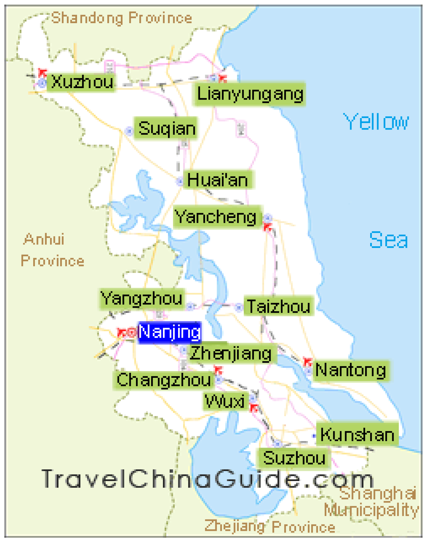
A map with the location of Jiangsu Province is provided as below in Figure 1.
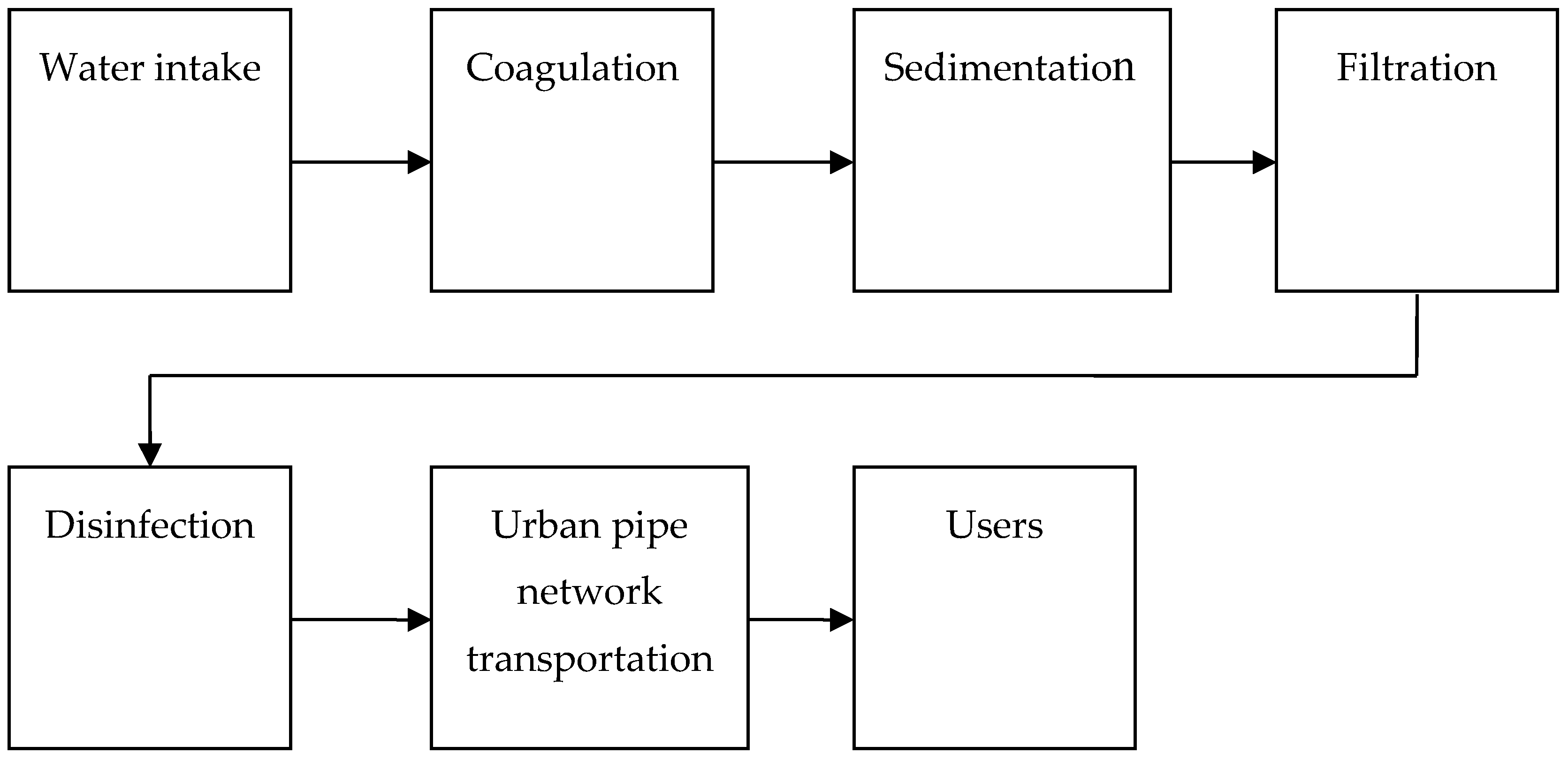
A schematic of water supply systems is presented as below in Figure 2.
Six cities in Jiangsu Province are selected for the research, namely, Nanjing (), Wuxi (), Nantong (), Yangzhou (), Xuzhou (), and Lianyungang (). Of the six cities, Nanjing is the capital of Jiangsu Province, Nanjing and Wuxi are located in the south of Jiangsu, Nantong and Yangzhou are located in the middle of Jiangsu, and Xuzhou and Lianyungang are located in the north of Jiangsu.
Referring to the technical and economic examples of water supply and drainage engineering (Liu and Shi [38]), the 2017 statistical yearbook of Jiangsu (Jiangsu Provincial Bureau of Statistics and Jiangsu Survey Office of National Bureau of Statistics of China [39]) and 2016 statistics bulletin on China’s water activities (Ministry of Water Resources of China [40]), we set the parameters of the above multiple urban domestic water systems as follows.
The time length for the simulation is set to 10 years, with .
Since decision matrices and of Equation (10), based on the asymptotic stability of the system at the origin of its equilibrium state, have solutions, the simulation system also represents the equilibrium state of the system at the origin. This can be done in the following ways.
For city , let us assume that is the target domestic water demand, is the target domestic water supply, is the difference between the actual domestic water demand and , and are the difference between the actual domestic water supply and . With this setting, if and reach and remain at the origin, it means that the actual values of domestic water demand and supply are equal to their target values, respectively, and the system therefore achieves asymptotic stability. Moreover, if the setting is , then the domestic water system for achieves a balance of supply and demand.
Under the above assumption and setting, we have
By substituting the above parameters into Equation (16) and applying MATLAB software, we can obtain the following feasible solutions:
By substituting the values of and into Equation (17), we obtain
The eigenvalues of are 0.0181 and 0.0185, and hence is a positive definite symmetric matrix. is the state feedback gain matrix.
By substituting the value of into Equation (18), we have
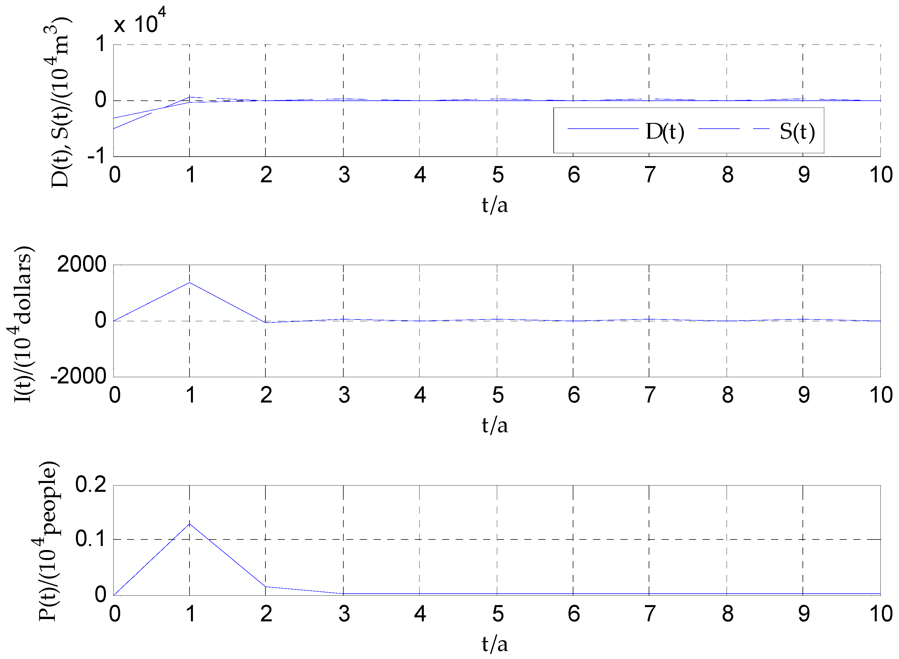
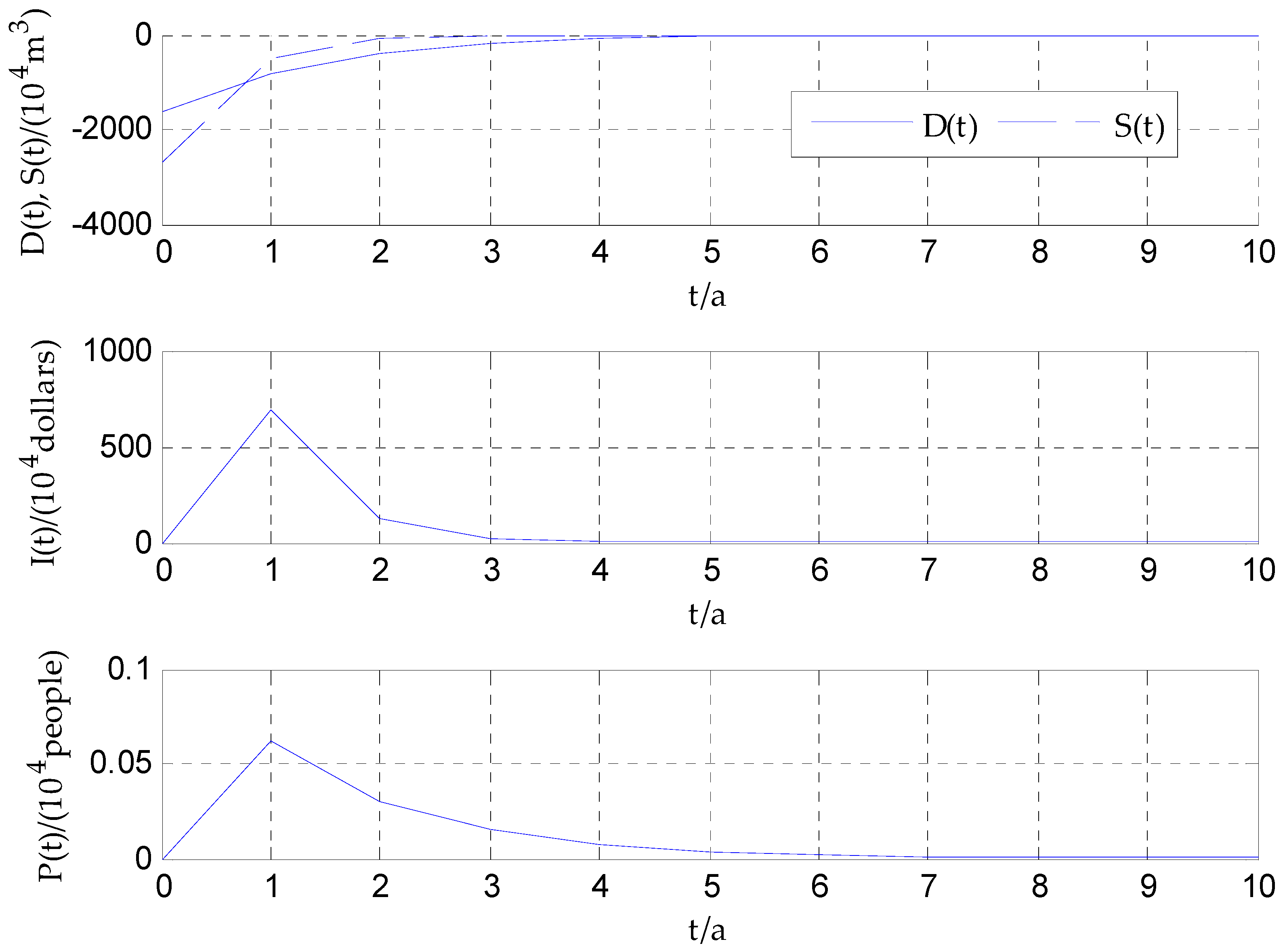
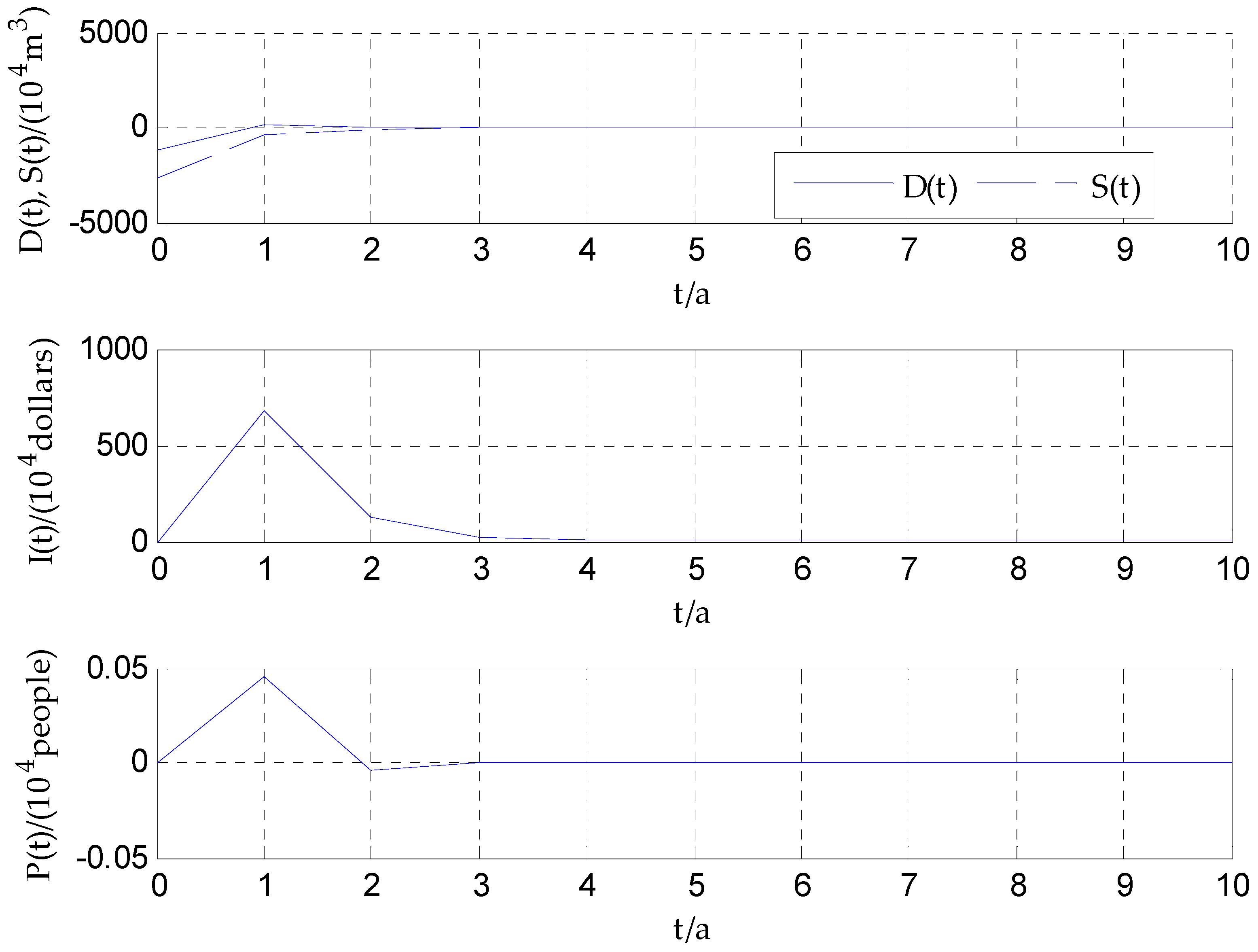
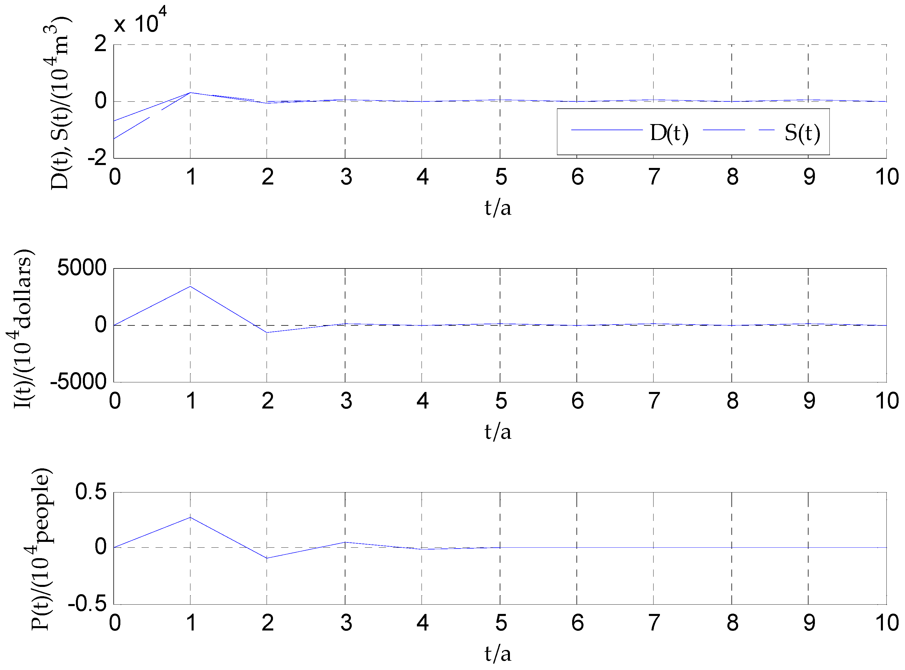
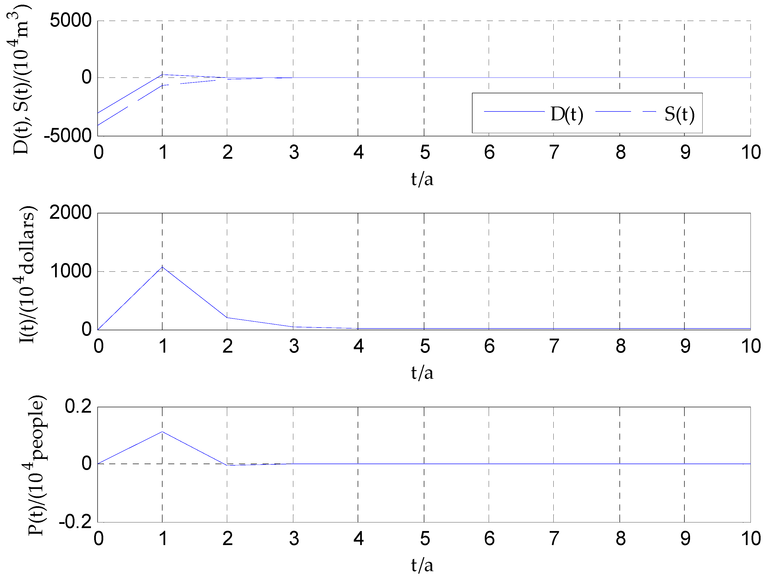
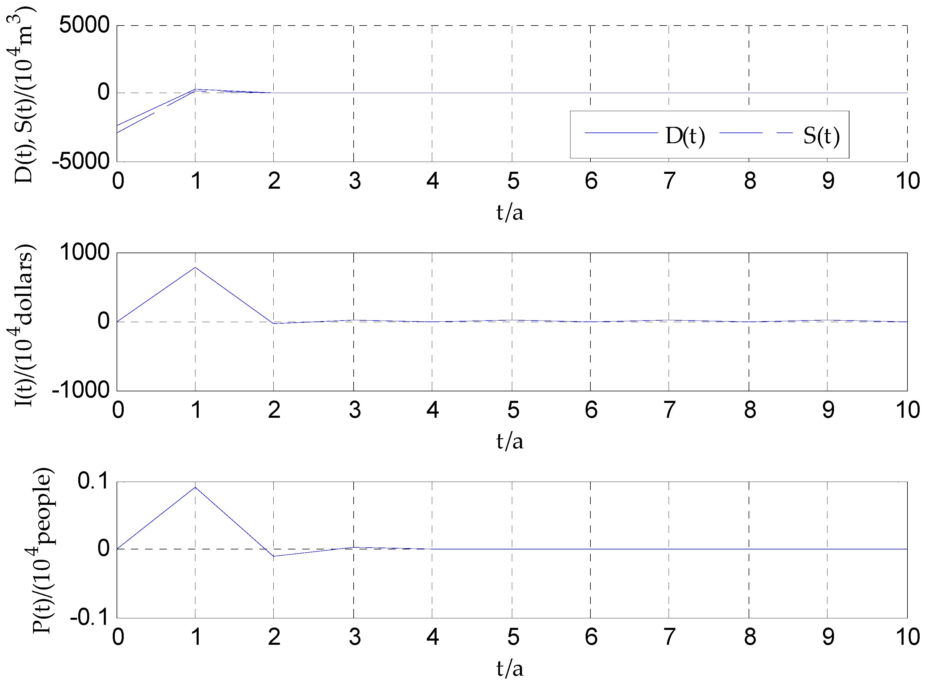
Equation (27) is the simultaneously stabilized robust control decision scheme for multiple urban domestic water systems. Figure 3, Figure 4, Figure 5, Figure 6, Figure 7 and Figure 8 show the simulation results.
The simulation results in Figure 3, Figure 4, Figure 5, Figure 6, Figure 7 and Figure 8 show that through the coordinated control of fixed capital investment and labor input , using the same control scheme of Equation (19), , these six urban domestic water systems with different parameters can achieve asymptotical stability and a balance between supply and demand.
All the simulation results in all the figures (i.e., all the cities) show mostly the same pattern, and supply and demand change mostly at . However, what seems suspicious is the fact that the cities are very different in their water use, and why is such uniformity here? The reasons for this uniformity are as follows. These cities are located in the same province, and they are considered to follow the demand equations and supply equations with the same structure but different parameters. Their water consumption parameters vary widely, such as in Equation (1). However, usually the system structure has a greater impact on system behavior than the parameters. Therefore, as they have the same structure, although the parameters vary greatly, these cities exhibit uniform dynamic characteristics when given and . Since the deviation between the initial state value and the target value is the largest, the control force is maximum at . Accordingly, the state value of demand and supply also varies maximally at , in order to make the state value tend to the target value as soon as possible. With the increase of , the control variable will decrease as the deviation between the state value and the target value becomes smaller. If more factors are taken into account in the demand model, and the structure of the demand function of each city is different, the system dynamics may not present such uniformity.
China also has a water shortage problem. This paper mainly studies how to control and after setting and , so that and can approach or even reach and , respectively. There is a premise to achieve this goal, that is, that can be achieved in reality. Under the condition of satisfying this premise, this paper can study the realization of system goals through the dynamic configuration of and . When , and S* exceeds the maximum water supply capacity in reality, it is impossible to achieve the goal of reaching . At this time, the water shortage state will exist.
5. Robustness of the Control Decision Method
For the case given in the preceding section, the following numerical calculation suggests that the control decision scheme of Equation (19) can still be effective and robust when the system parameters change.
Let us suppose that in the preceding section, the relevant cities have the following changes to some of their parameters, as presented in Table 2.
The remaining parameters remain unchanged.
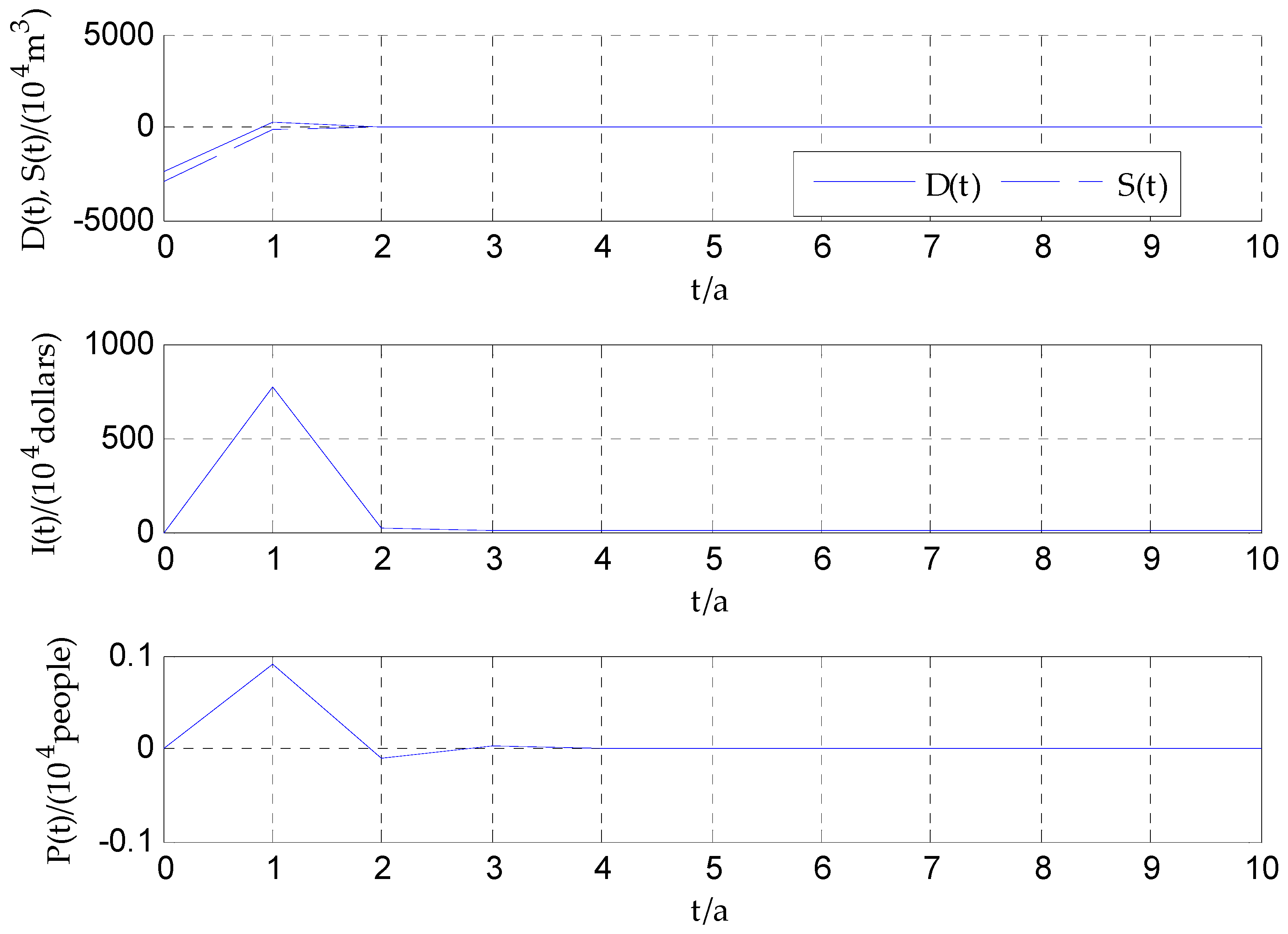
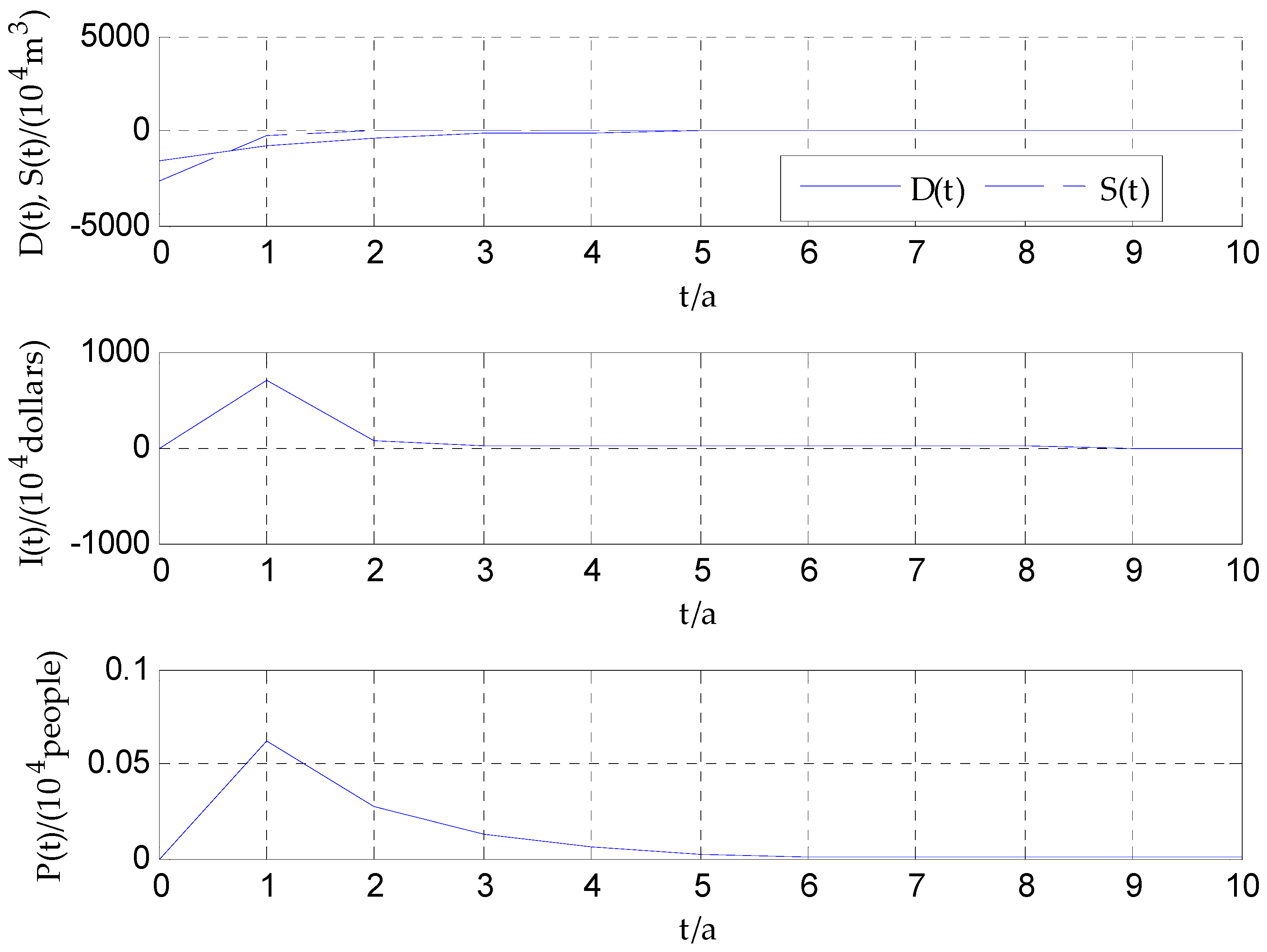
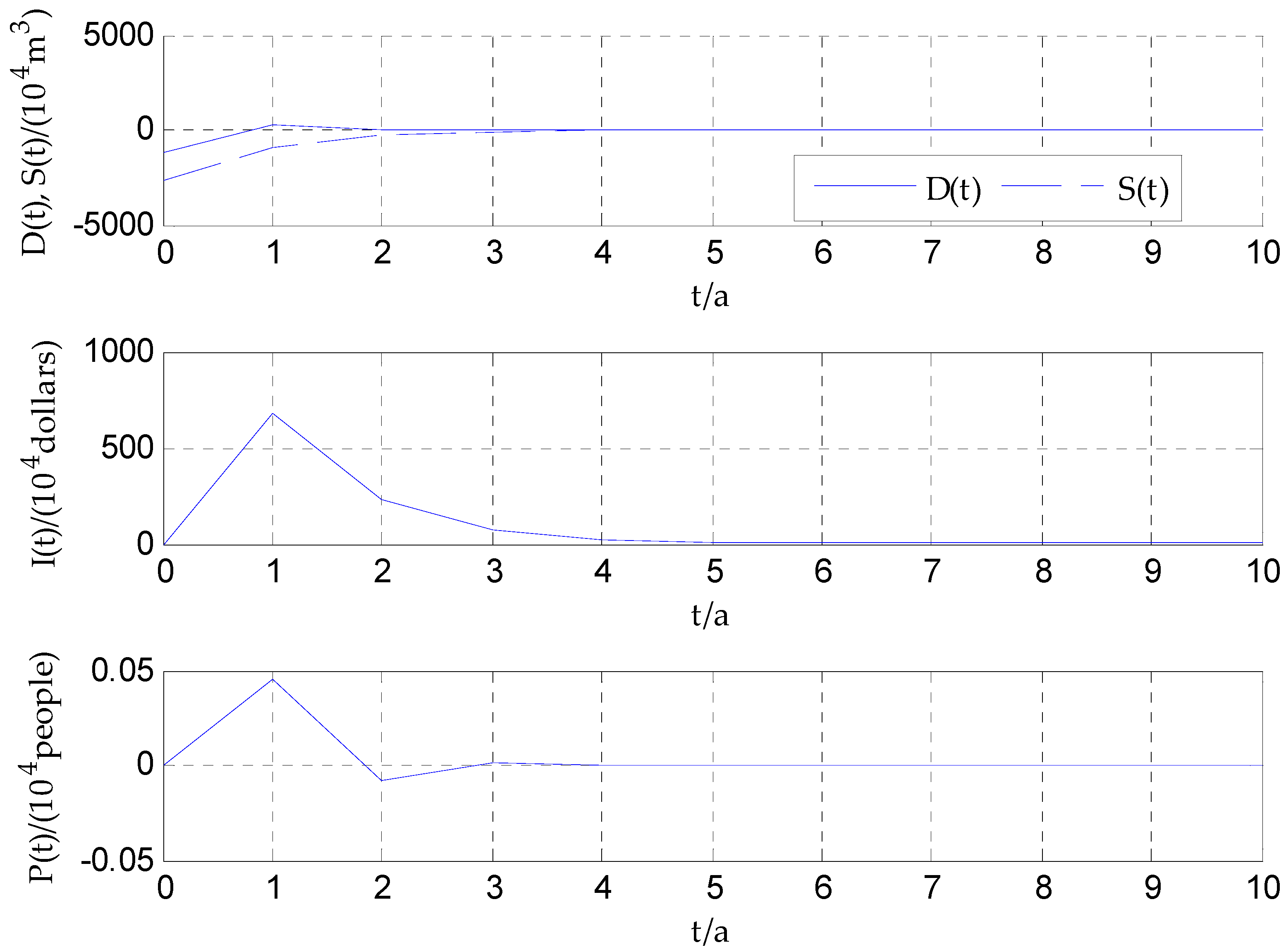
Equation (19) is again adopted to make control decisions for the urban domestic water system. The simulation results are shown in Figure 9, Figure 10, Figure 11, Figure 12, Figure 13 and Figure 14.
Figure 9, Figure 10, Figure 11, Figure 12, Figure 13 and Figure 14 suggest that, although some system parameters have changed, the control decision scheme of Equation (19) remains effective and can adapt to such changes. Each city still achieves the goal of supply and demand balance and asymptotic stability, indicating that the control decision scheme is robust to system parameter changes.
Since the state feedback gain matrix is obtained according to the parameters before the change in the preceding section, the time for the asymptotic stability of the system in the present section is generally longer than that in the preceding section.
When the system parameters, , change significantly, if we continue to use Equation (19) for the control decisions, this may lead to a situation in which some cities are unable to achieve their control goal of asymptotical stability. When such a situation occurs in the simulation results, for the system with changed parameters, we should use Equation (16) to resolve the linear matrix inequalities for and , and try to find a new feasible solution for and .
In the case of demonstrating robustness, parameter value changes are deliberately chosen to differ greatly from the original value. For example, . If the control scheme is still valid under the condition of a 700% increase, the system control scheme is also effective when the change in the parameter value is smaller, such as only increasing by 10%. This proves that the system has considerable robustness to parameter value variation. To describe the nonlinear and the trade-off problems in water systems, other models are needed.
Finally, it should be pointed out that there are some limitations to this study. One is that the production function involves the two commonly used production factors of investment and labor, but does not take into account the influence of other production factors, such as the technical level, which may also play a relatively minor role in the production. Another is that the method developed requires a common solution for multiple urban domestic water systems, that is, decision matrices and of Equation (10) have solutions. If the parameters of a multiple urban domestic water system vary largely, such that decision matrices and of Equation (10) have no feasible solutions, this method is no longer applicable.
6. Conclusions
Differences in economic and social development and geographical conditions among cities lead to different parameter values for multiple urban domestic water supply and demand systems. From the perspective of sustainable development, all urban domestic water supply and demand systems should achieve asymptotic stability and a balance between supply and demand.
Since fixed capital investment and labor input are commonly used production factors, it is appropriate to take them as control variables to make simultaneously stabilized robust control decisions for multiple urban domestic water systems.
The comparison between the model developed in this paper and the existing models is as follows.
In Reference [9], an optimal control model of water supply investment based on the time series of the urban water demand function is developed. The urban water demand in the model is both growing and seasonal. The control variables used in this model only relate to investment, without considering the labor force factors. In Reference [10], the static share coefficient method, which is commonly used to calculate water supply benefit, is dynamic, and an optimal control model of urban water supply investment based on the dynamic share coefficient method is proposed. The control variables used in this model also only relate to investment, without considering labor force.
However, when calculating the impact of production factors on output, labor force is usually one of the important factors to be considered in addition to investment (Romer [31]). Therefore, when establishing the control decision model of the urban water supply input, the model will be more comprehensive if labor is considered as a production factor.
In addition, although there are quite perfect theories, even for fairly simple problems, the analysis and solution of the optimal control model can be very complicated. Therefore, the parameters in the optimal control model are usually assumed to be invariant (Chiang [41]). The above two models also retain this assumption.
However, due to fluctuations in factors such as climate and population, the parameters of urban water supply systems may fluctuate rather than remain unchanged. For the case in which the system parameters are uncertain, establishing a robust control model for the water supply system becomes more adaptive.
In order to address the limitations of existing models fail to investigate the influence of labor force and the uncertainty of parameters, a robust economic control model for the urban domestic water uncertain system is established in Reference [16]. This model simultaneously takes into account the impact of two production factors—investment and labor—on the water supply system. Meanwhile, the system can be balanced using the robust control method under the condition of parameter fluctuation.
The model established in this paper also considers the impact of the two production factors of investment and labor on the water supply system, but this model differs from the model in Reference [16] in the following aspects.
First, the water demand function is different. In Reference [16], urban domestic water demand is described using a time series function of growth and seasonality, which belongs to the trend prediction method. In contrast, the urban domestic water demand in this paper is designed to be the product of the urban domestic water consumption population and per capita domestic water consumption, and this belongs to the quota forecasting method. Both of these methods are the main methods currently used for water demand prediction. Importantly, China’s water industry standards recommend that domestic water demand be estimated using the per capita daily water consumption index [25]. Therefore, the domestic water demand function in this paper is more in line with the technical specifications of China’s water industry standards.
Second, the scope of application is different. In Reference [16], the model is only for the single urban domestic water system, and the multiple urban simultaneous control decision problem is not considered. In contrast, the model developed in this paper is applicable not only to the single urban domestic water system, but also to the simultaneous control of multiple urban domestic water systems. This difference expands the scope of application of the control decision method.
Third, the control decision method is different. In Reference [16], the urban water system is balanced through the pole placement method. This method requires the design of a complex compensator subsystem, which may not be easy to implement in practical applications. In contrast, the model in this paper adopts a simultaneously stabilized control method based on the Lyapunov stability theory and linear matrix inequality; it does not need to design a compensator, and hence the solutions to applications are relatively simple.
Therefore, in terms of usability, the model in this paper has certain advantages in terms of being easier to operate.
In this paper, a simultaneously stabilized control decision method based on the Lyapunov stability theory and linear matrix inequality is developed. Compared with the control method that makes the system asymptotically stable through pole placement, the proposed method does not necessarily need to design a complex compensator subsystem, and the solution to an application becomes simpler. Therefore, the method of this paper has the advantage of being easier to implement and operate.
The results of the activity are interpreted and deliver the following meanings. Firstly, from the simulation results, it can be seen that although the parameters of these cities differ greatly, because their systems have the same structure, they show uniform dynamic characteristics when given similar control schemes. It can be concluded that the influence of system structure on system dynamic behavior is usually greater than that of parameters. Secondly, the simulation results also show that the control variable is the largest in the initial stage of simulation, and is then gradually reduced. This is because the deviation between the state value and the target value is the largest in the initial stage, and the maximum control force is used to help the state value quickly tend to the target value; moreover, with the deviation between the state value and the target value becoming smaller, it is no longer necessary to have such a large control force as in the initial stage, so the control variable thereafter is reduced.
The control decision method of this paper is of particular reference value to the following situation: To reduce the difficulty of control, an administrative agency makes a unified decision for the domestic water system in different areas under its jurisdiction. By making unified decisions on domestic water investment and labor input in different regions, all the domestic water systems in the various regions can achieve stable operation.
One limitation to this study is that it does not reflect the influence of any production factors except for investment and labor input. Another is that it requires a common solution for multiple urban domestic water systems.
The novelty of the method distinguished in this paper is as follows. Since existing research has focused on the management of water resources in a single region, the simultaneous management of multiple regions is less involved. However, it is possible to manage water resources in multiple regions simultaneously, especially for urban water management under a central management system such as China. This paper studies this situation. For water systems in different cities, the same control scheme can be used for the simultaneous control of investment and labor input, as shown in Equation (18). This can reduce the control complexity of different cities. However, due to the complexity of the economic control method, the method proposed in this paper has not been implemented in practice. The effectiveness of the method can only be verified through simulation. This is also a deficiency of this paper.
Author Contributions
K.L. conceived and designed the model; K.L. and T.M. performed the case simulation and analyzed the data; K.L. wrote the paper; and G.W. reviewed and edited the manuscript. All the co-authors contributed substantially to the work reported.
Funding
This research was funded by the National Social Science Foundation of China (grant number 17BGL220), the Humanities and Social Science Youth Foundation of Ministry of Education of China (grant number 14YJCZH074), the Philosophical and Social Science Foundation of Jiangsu Higher Education Institutions of China (grant number 2014SJB060), a Project Funded by the Priority Academic Program Development of Jiangsu Higher Education Institutions (PAPD), the Top-notch Academic Programs Project of Jiangsu Higher Education Institutions (TAPP), and partially supported by the HRSA, US DHHS (grant number H49MC00068).
Conflicts of Interest
The authors declare no conflict of interest.
Appendix A
Proof of Theorem 1.
Below, we will perform some transformations for Equations (1)–(5) to obtain a clearer description of the relationship between , and , , , and .
Substituting Equation (5) into Equation (1), we have
and
From Equations (4), (A1) and (A2), we have
Equation (2) then implies
From Equations (A1) and (A4), we have
From Equations (2), (3), (A1) and (A5), it holds that
From Equations (4), (A1), (A2) and (A6), we obtain
From Equation (A7), we have
By writing Equations (A3) and (A8) in the matrix form, the domestic water supply and demand system model of city is given by
Therefore, Equation (6) is proved. □
References
- National Bureau of Statistics of China. 2017 China Statistical Yearbook; China Statistics Press: Beijing, China, 2017.
- Wang, H. Research on China’s Water Resources Issues and Sustainable Development Strategy; China Electric Power Press: Beijing, China, 2010. [Google Scholar]
- Mourad, E.; Lachhab, A.; Limouri, M.; Dahhou, B.; Essaid, A. Adaptive control of a water supply system. Control Eng. Pract. 2001, 9, 343–349. [Google Scholar] [CrossRef]
- Sahu, M.K.; Gupta, A.D. Reservoir operation and evaluation of downstream flow augmentation. J. Am. Water Resour. Assoc. 2001, 37, 675–684. [Google Scholar] [CrossRef]
- Eker, I.; Grimble, M.J.; Kara, T. Operation and simulation of city of gaziantep water supply system in turkey. Renew. Energy 2003, 28, 901–916. [Google Scholar] [CrossRef]
- Roseta-Palma, C.; Xepapadeas, A. Robust control in water management. J. Risk Uncertain. 2004, 29, 21–34. [Google Scholar] [CrossRef]
- Fang, Q.; Wang, X.J. Application of the maximum principle with state constraints to reservoir operation. Acta Autom. Sin. 2006, 32, 767–773. [Google Scholar]
- Li, K.B.; Chen, S.F. Robust control of the investment in urban water supply and demand system. J. Syst. Sci. Math. Sci. 2010, 30, 22–32. [Google Scholar]
- Li, K.B.; Chen, S.F. Control and simulation of urban water supply and demand discrete system’s investment. J. Syst. Simul. 2010, 22, 1746–1751. [Google Scholar]
- Li, K.B. Town water supply investment control and simulation model based on dynamic share coefficient method. Syst. Eng. Theory Pract. 2011, 31, 158–164. [Google Scholar]
- Li, K.B. Dynamic optimization and simulation of urban domestic water based on logistic and c-d function. J. Shanghai Jiaotong Univ. 2015, 49, 178–183. [Google Scholar]
- Pereira, M.; de la Peña, D.M.; Limon, D.; Alvarado, I.; Alamo, T. Application to a drinking water network of robust periodic mpc. Control Eng. Pract. 2016, 57, 50–60. [Google Scholar] [CrossRef]
- Sarbu, I.; Ostafe, G. Optimal design of urban water supply pipe networks. Urban Water J. 2016, 13, 521–535. [Google Scholar] [CrossRef]
- Qaderi, F.; Babanezhad, E. Prediction of the groundwater remediation costs for drinking use based on quality of water resource, using artificial neural network. J. Clean. Prod. 2017, 161, 840–849. [Google Scholar] [CrossRef]
- Nguyen, K.A.; Stewart, R.A.; Zhang, H.; Sahin, O.; Siriwardene, N. Re-engineering traditional urban water management practices with smart metering and informatics. Environ. Model. Softw. 2018, 101, 256–267. [Google Scholar] [CrossRef]
- Li, K.B.; Ma, T.Y.; Wei, G. Robust economic control decision method of uncertain system on urban domestic water supply. Int. J. Environ. Res. Public Health 2018, 15, 649. [Google Scholar] [CrossRef] [PubMed]
- Kohan-Sedgh, P.; Khayatian, A.; Asemani, M.H. Conservatism reduction in simultaneous output feedback stabilisation of linear systems. IET Control Theory Appl. 2016, 10, 2243–2250. [Google Scholar] [CrossRef]
- Gündeş, A.N.; Nanjangud, A. Simultaneous stabilization and constant reference tracking of LTI, MIMO systems. Asian J. Control 2013, 15, 1001–1010. [Google Scholar] [CrossRef]
- Chen, S.S.; Chang, Y.C.; Su, S.F. Lmi approach to simultaneous output-feedback stabilization for discrete-time interval systems. J. Chin. Inst. Eng. 2004, 27, 49–53. [Google Scholar] [CrossRef]
- Al-Awami, A.T.; Abdel-Magid, Y.L.; Abido, M.A. Simultaneous stabilization of power system using UPFC-based controllers. Electr. Power Compon. Syst. 2006, 34, 941–959. [Google Scholar] [CrossRef]
- Ryan, E.P. On simultaneous stabilization by feedback of finitely many oscillators. IEEE Trans. Autom. Control 2015, 60, 1110–1114. [Google Scholar] [CrossRef]
- Wang, Y.; Miao, Z.; Zhong, H.; Pan, Q. Simultaneous stabilization and tracking of nonholonomic mobile robots: A lyapunov-based approach. IEEE Trans. Control Syst. Technol. 2015, 23, 1440–1450. [Google Scholar] [CrossRef]
- Kaneko, O. Simultaneous stabilization problem in a behavioral framework. In Mathematical Control Theory II; Belur, M.N., Camlibel, M.K., Rapisarda, P., Scherpen, J.M.A., Eds.; Springer International Publishing: Cham, Switzerland, 2015; pp. 65–80. [Google Scholar]
- Baumann, D.D.; Boland, J.J.; Hanemann, W.M. Urban Water Demand Management and Planning; Chemical Industry Press: Beijing, China, 2005. [Google Scholar]
- Ministry of Water Resources of China. Water Conservancy Industry Standards of China: Technical Specification for the Analysis of Supply and Demand Balance of Water Resources (sl 429-2008); China Water & Power Press: Beijing, China, 2011.
- Xu, X.Y.; Wang, H.R.; Liu, H.J.; Li, J.Q.; Pang, B.; Xu, F. Assessment Report on Water Utilization Efficiency in China; Beijing Normal University Press: Beijing, China, 2010. [Google Scholar]
- Cui, Y.C. Handbook for Urban and Industrial Water Saving; Chemical Industry Press: Beijing, China, 2002. [Google Scholar]
- Guizhou Provincial Bureau of Statistics; NBS Survey Office in Guizhou. 2017 Statistical Yearbook of Guizhou; China Statistics Press: Beijing, China, 2017.
- Hunan Provincial Bureau of Statistics. 2017 Hunan Statistical Yearbook; China Statistics Press: Beijing, China, 2017.
- Guangzhou Municipal Statistics Bureau; Guangzhou Survey Office of National Bureau of Statistics. 2017 Guangzhou Statistical Yearbook; China Statistics Press: Beijing, China, 2017.
- Romer, D. Advanced Macroeconomics; The Commercial Press: Beijing, China, 2004. [Google Scholar]
- Spulber, N.; Sabbaghi, A. Economics of Water Resources: From Regulation to Privatization; Shanghai People’s Publishing House: Shanghai, China, 2010. [Google Scholar]
- Liu, C.G.; Zhang, X.P. The influence of labor force ratio on the investment rate and economic growth: Based on the research of solow model and data of china. J. Xiangtan Univ. (Philos. Soc. Sci.) 2016, 40, 60–65. [Google Scholar]
- Li, Y.H.; Luo, L.H. Demographic dividend, cross-industry configuration of labors and sustainable economic growth. Econ. Probl. 2016, 4, 13–20. [Google Scholar]
- Haie, N.; Keller, A.A. Macro, meso, and micro-efficiencies and terminologies in water resources management: A look at urban and agricultural differences. Water Int. 2014, 39, 35–48. [Google Scholar] [CrossRef]
- Yu, L. Modern Control Theory; Tsinghua University Press: Beijing, China, 2011. [Google Scholar]
- Zhang, D.W. Robust Analysis and Synthesis of Uncertain Systems—Matrix Inequality Method; National Defense Industry Press: Beijing, China, 2014. [Google Scholar]
- Liu, J.L.; Shi, X.G. Analysis and Application of Technical and Economic Examples of Water Supply and Drainage Engineering; Chemical Industry Press: Beijing, China, 2004. [Google Scholar]
- Jiangsu Provincial Bureau of Statistics; Jiangsu Survey Office of National Bureau of Statistics of China. 2017 Statistical Yearbook of Jiangsu; China Statistics Press: Beijing, China, 2017.
- Ministry of Water Resources of China. 2016 Statistics Bulletin on China Water Activities; China Water & Power Press: Beijing, China, 2017.
- Chiang, A.C. Elements of Dynamic Optimization; The Commercial Press: Beijing, China, 2003. [Google Scholar]
Figure 1.
Location of Jiangsu Province (https://www.travelchinaguide.com/images/map/jiangsu/jiangsu-s.gif).
Figure 1.
Location of Jiangsu Province (https://www.travelchinaguide.com/images/map/jiangsu/jiangsu-s.gif).

Figure 2.
Schematic of water supply systems.

Figure 3.
Simulation results for .

Figure 4.
Simulation results for .

Figure 5.
Simulation results for .

Figure 6.
Simulation results for .

Figure 7.
Simulation results for .

Figure 8.
Simulation results for .

Figure 9.
Simulation results after the change to the parameters of .

Figure 10.
Simulation results after the change to the parameters of .

Figure 11.
Simulation results after the change to the parameters of .

Figure 12.
Simulation results after the change to the parameters of .

Figure 13.
Simulation results after the change to the parameters of .

Figure 14.
Simulation results after the change to the parameters of .


Table 1.
Parameters of the case.
| 0.004 | 114 | 0.80 | 0.20 | 0.06 | 0.80 | 0.060 | 0.90 | 85,000 | −7000 | −13,625 | |
| 0.003 | 79 | 0.75 | 0.25 | 0.06 | 0.76 | 0.048 | 0.85 | 25,000 | −3400 | −5219 | |
| 0.002 | 66 | 0.70 | 0.30 | 0.05 | 0.78 | 0.072 | 0.80 | 15,000 | −3000 | −4165 | |
| 0.002 | 77 | 0.72 | 0.28 | 0.05 | 0.72 | 0.040 | 0.75 | 12,000 | −2400 | −2987 | |
| 0.003 | 45 | 0.65 | 0.35 | 0.03 | 0.68 | 0.048 | 0.82 | 11,000 | −1640 | −2699 | |
| 0.002 | 71 | 0.68 | 0.32 | 0.04 | 0.65 | 0.036 | 0.78 | 9000 | −1200 | −2633 |
Table 2.
Changes to the parameters.
| 0.032 | 125.4 | ||||||
| 0.0033 | 63.2 | ||||||
| 0.56 | 0.33 | ||||||
| 0.792 | 0.224 | ||||||
| 0.748 | 0.0384 | 0.902 | |||||
| 0.52 | 0.0396 | 0.858 |
© 2018 by the authors. Licensee MDPI, Basel, Switzerland. This article is an open access article distributed under the terms and conditions of the Creative Commons Attribution (CC BY) license (http://creativecommons.org/licenses/by/4.0/).
Share and Cite
MDPI and ACS Style
Li, K.; Ma, T.; Wei, G. Multiple Urban Domestic Water Systems: Method for Simultaneously Stabilized Robust Control Decision. Sustainability 2018, 10, 4092. https://0-doi-org.brum.beds.ac.uk/10.3390/su10114092
AMA Style
Li K, Ma T, Wei G. Multiple Urban Domestic Water Systems: Method for Simultaneously Stabilized Robust Control Decision. Sustainability. 2018; 10(11):4092. https://0-doi-org.brum.beds.ac.uk/10.3390/su10114092
Chicago/Turabian StyleLi, Kebai, Tianyi Ma, and Guo Wei. 2018. "Multiple Urban Domestic Water Systems: Method for Simultaneously Stabilized Robust Control Decision" Sustainability 10, no. 11: 4092. https://0-doi-org.brum.beds.ac.uk/10.3390/su10114092
Note that from the first issue of 2016, this journal uses article numbers instead of page numbers. See further details here.