Economic Impact of the High-Speed Railway on Housing Prices in China

Abstract

This study investigated whether and to what extent does the High-Speed Railway (HSR) affect city-level housing prices. With the data of HSR operation and housing prices from 285 cities from 2009 to 2017, the paper aimed to estimate the quantitative relationship between HSR and city-level housing prices and exploited city and regional dummy variables to assess the disparities between regions, followed by the economic effects between typical city pairs. Our findings were as follows: (1) The introduction of HSR leads to a 13.9% increase in city-level housing prices, and the figures for national central cities and regional central cities were 31.7% and 19.6%, respectively; (2) regional imbalance was mitigated with the development of the HSR, and some central cities in underdeveloped regions were stimulated with regard to housing price growth; (3) siphon effects and diffusion effects were observed in megacity–small city pairs, while synergistic effects often lay in megacity–megacity pairs, and such effects all tended to be more significant with increases in the number of HSR lines and a drop in the travel time.

1. Introduction

To narrow regional imbalance is an important goal of sustainable economic development, especially in developing nations. With rapid economic growth following the opening-up policy, regional economic disparity has become a major challenge in China [1]. For instance, from 1978 to 1998, provinces located along the eastern and southern coast, such as Fujian and Guangdong, experienced very fast economic development, with an average annual real GDP growth rate of more than 10%, whereas the figures for other inland provinces, such as Gansu and Guizhou, were much slower, with an average growth rate of 6% [2]. In the most recent two decades, the disparity between different regions in China has expanded. Such an increased regional inequality has raised numerous concerns about social stability and economic sustainability [3].

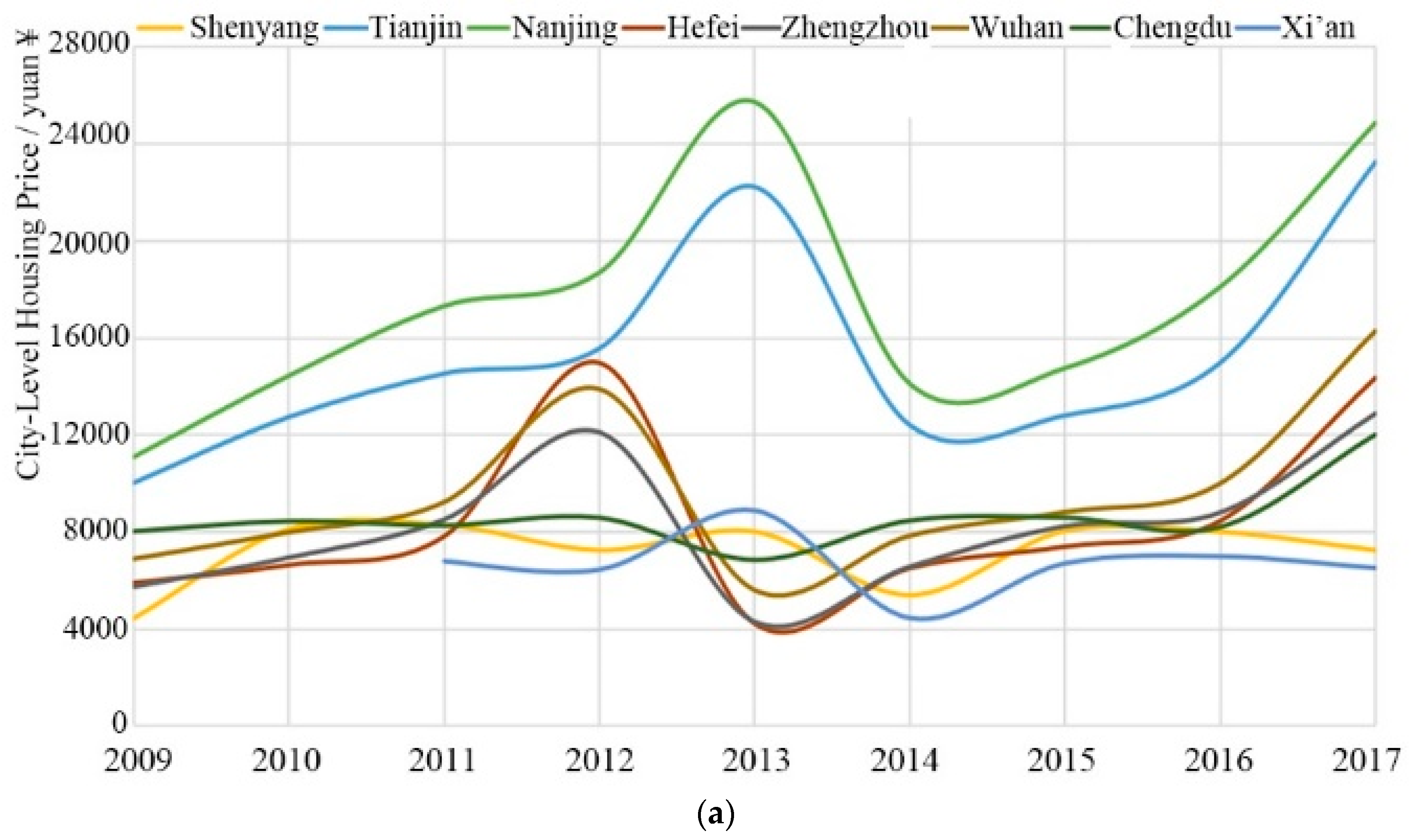
To address these challenges, the Chinese central government launched a series of policies to promote a coordinated regional economic development. Prime Minister Li Keqiang revealed that further development was not only critical to China’s economic success, but a fundamental way to reduce regional disparities [4]. Similarly, national High-Speed Railway (HSR) corridors in China were initiatively designed to reduce regional disparity by connecting the developed east and south coastal provinces [5], and therefore the implementation effect of the HSR network on this issue was worth evaluating [3]. The gap in housing price growth between cities and regions can result in direct social inequality, and the economic distribution effects of the construction of transport infrastructure exert similar consequences, and statistically, both of them have shown similar changes, fluctuating in 2012 and 2013 and increasing sharply after 2016 (Figure 1). In the last decade, housing price appreciation has been phenomenal in major Chinese cities, leading to concerns of real estate price bubbles and housing affordability as well as surges in assets for many Chinese households. For instance, Zheng and Saiz [6] found that Beijing had an annual average appreciation rate of 27.4%, and that the average annual growth for 35 cities was 14.3% between 2006 and 2013. In the meantime, China’s HSR construction has been booming, and more and more Chinese can enjoy the convenience and accessibility improvements of HSR lines [3,7,8]. By the end of 2017, the operating mileage of China’s railways nationwide was 127,000 km, of which 25,000 km was HSR lines, thereby accounting for about 66.3% of the global total operating mileage. Figure 1a shows the city-level housing price growth in China’s high-speed rail hub cities (2009–2017), and Figure 1b illustrates the operating mileage and year-on-year increase of China’s HSR (2009–2025). The development history of HSR network in China can be divided into three scenarios (details in

Table A1. Introduction of China’s HSR network system (from the past to the future).

Scenario	Typical Year	Important Event
Period of China Railwayline being upgraded for HSR (2003–2007).	2003	The first upgraded line began operating.
	2007	The second upgraded line operated.
		The sixth round of the Railway Speed-Up Campaign, during which 6849 km of CR lines were upgraded to speeds of over 200 km/h.
Period of newly built HSR lines expansion (2008–2015).	2008	The Mid to Long-Term Railway Network Plan of China’s Ministry of Railways (2008) was issued.
		The first newly built HSR line, from Beijing to Tianjin, operated.
	2008–2015	The HSR network expanded rapidly and newly built HSR lines were introduced annually and on a massive scale:
	2015	The “four north-south and four west-east corridors” national HSR network was basically completed by the end of 2015.
Period of realizing a miraculous national HSR network (2016–2025).	2016	The Mid to Long-Term Railway Network Plan (revised in 2016).
	2025	Formulating the “eight vertical and eight horizontal corridors” national HSR network.

Source: Authors collected data according to the website of the National Railway Administration of the People’s Republic of China, http://www.nra.gov.cn/.

), and we have also collected detailed information for HSR lines used in our dataset from 2009 to the end of 2017(details in

Table A2. HSR lines in use from 2009 to the end of 2017.

HSR Lines	Construction Time	Opening Time	Length (km)	Speed (km/h)
Qinhuangdao–Shenyang	01/01/1999	01/07/2003	405	250
Hefei–Nanjing	11/06/2005	19/04/2008	154	250
Beijing–Tianjin	07/04/2005	01/08/2008	120	350
Qingdao–Jinan	28/01/2007	20/12/2008	393	250
Shijiazhuang–Taiyuan	11/06/2005	01/04/2009	190	250
Hefei–Wuhan	01/08/2005	01/04/2009	351	200
Dazhou–Chengdu	01/05/2005	07/07/2009	148	250
Ningbo–Taizhou–Wenzhou	27/10/2005	28/09/2009	268	250
Wenzhou–Fuzhou	08/01/2005	28/09/2009	298	250
Wuhan–Guanghzou	23/06/2005	26/12/2009	968	350
Zhengzhou–Xian	01/09/2005	06/01/2010	455	350
Fuzhou–Xiamen	01/10/2005	26/04/2010	275	250
Chengdu–Dujiangyan	04/11/2008	12/05/2010	65	250
Shanghai–Nanjing	01/07/2008	01/07/2010	301	220
Nanchang–Jiujiang	28/06/2007	20/09/2010	131	350
Shanghai–Hangzhou	01/04/2009	26/11/2010	150	350
Yichang–Wanzhou	01/12/2003	22/12/2010	377	200
Wuhan–Yichang	17/09/2008	23/12/2010	293	250
Haikou–Sanya (eastern coastal line)	29/09/2007	30/12/2010	308	250
Changchun–Jilin	01/04/2008	30/12/2010	111	200
Jiangmen–Xinhui	18/12/2005	07/01/2011	27	350
Beijing–Shanghai	18/04/2008	30/06/2011	1433	350
Guangzhou–Shenzhen	20/08/2008	26/12/2011	116	200
Longyan–Xiamen	25/12/2006	01/07/2012	171	350
Zhengzhou–Wuhan	15/10/2008	28/09/2012	536	350
Hefei–Bengbu	20/05/2009	16/10/2012	132	350
Haerbin–Dalian	23/08/2007	01/12/2012	921	350
Beijing–Zhengzhou	26/12/2007	26/12/2012	693	350
Nanjing–Hangzhou	01/04/2009	01/07/2013	249	350
Panjin–Yinkou	31/05/2009	12/09/2012	89	350
Tianjin–Qinghuangdao	08/11/2008	01/12/2013	261	350
Xiamen–Shenzhen	23/11/2007	28/12/2013	502	250
Xian–Baoji	18/12/2009	28/12/2013	148	250
Guangxi Coastal (Nanning–Qinzhou–Beihai)	11/12/2008	28/12/2013	261	250
Liuzhou–Nanning	27/12/2008	28/12/2013	223	350
Wuhan–Xianning	26/03/2009	28/12/2013	90	250
Taiyuan–Xian	03/12/2009	01/07/2014	678	250
Nanchang–Changsha	26/02/2009	16/09/2014	344	350
Hangzhou–Nanchang	18/04/2010	10/12/2014	582	350
Lanzhou–Wulumuqi	01/01/2010	26/12/2014	1776	250
Guangzhou–Nanning	11/09/2008	18/04/2014	577	250
Huanggang–Wuhan–Huangshi	02/10/2009	18/06/2014	97	250
Taiyuan(south)–Xi’an(north)	03/12/2009	01/07/2014	579	250
Nanchang(west)–Changsha(south)	22/12/2009	16/09/2014	342	300
Urumqi (south)–Hami	04/11/2009	16/11/2014	530	200
Hangzhou (east)–Nanchang (west)	22/12/2009	10/12/2014	591	300
Changsha (south)–Xinhuang (west)	16/03/2010	16/12/2014	420	300
Chengdu–Mianyang–Leshan	30/12/2008	20/12/2014	319	200
Wuzhou (south) –Guangzhou (south)	09/11/2008	26/12/2014	249	200
Guizhou–Guangxi	13/10/2008	26/12/2014	861	250
Hami–Lanzhou (west)	04/11/2009	26/12/2014	1246	200
Zhengzhou–Songcheng	29/12/2009	28/12/2014	50	200
Xinhuang (west) –Guiyang (north)	26/03/1010	18/06/2015	286	300
Harbin–Qiqihar	05/07/2009	17/08/2015	286	250
Nanjing (south)–Anqing	28/12/2008	06/12/2015	257	200
Nanning–Baise	27/12/2009	11/12/2015	223	200
Chengdu–Chongqing	22/03/2010	26/12/2015	305	300
Shenzhen–Futian	20/08/2008	30/12/2015	8	300
Zhengzhou–Xuzhou	26/12/2 012	10//9/2016	357	300
Chongqing (north)–Wanzhou (north)	22/12/2010	28/11/2016	247	200
Guiyang–Kunming	26/03/2010	28/12/2016	461	300
Baise–Kunming (south)	27/12/2009	28/12/2016	487	200
Dazhi (north)–Yangxin	29/12/2013	12/06/2017	36	200–250
Baoji–Lanzhou	19/10/2010	09/07/2017	403	250
Hohhot (east)–Wulanchabu	16/06/2014	03/08/2017	126	250
Yangxin–Jiujiang	29/12/2013	21/09/2017	79	250
Jiangyou–Xi’an	10/11/2010	06/12/2017	509	250
Shijiazhuang–Jinan	08/02/2014	28/12/2017	319	250

Notes: Data were obtained from the “Major Events” and the “Finished and Ongoing Projects” sections of the China Railway Yearbooks from 1999 to 2017.

).

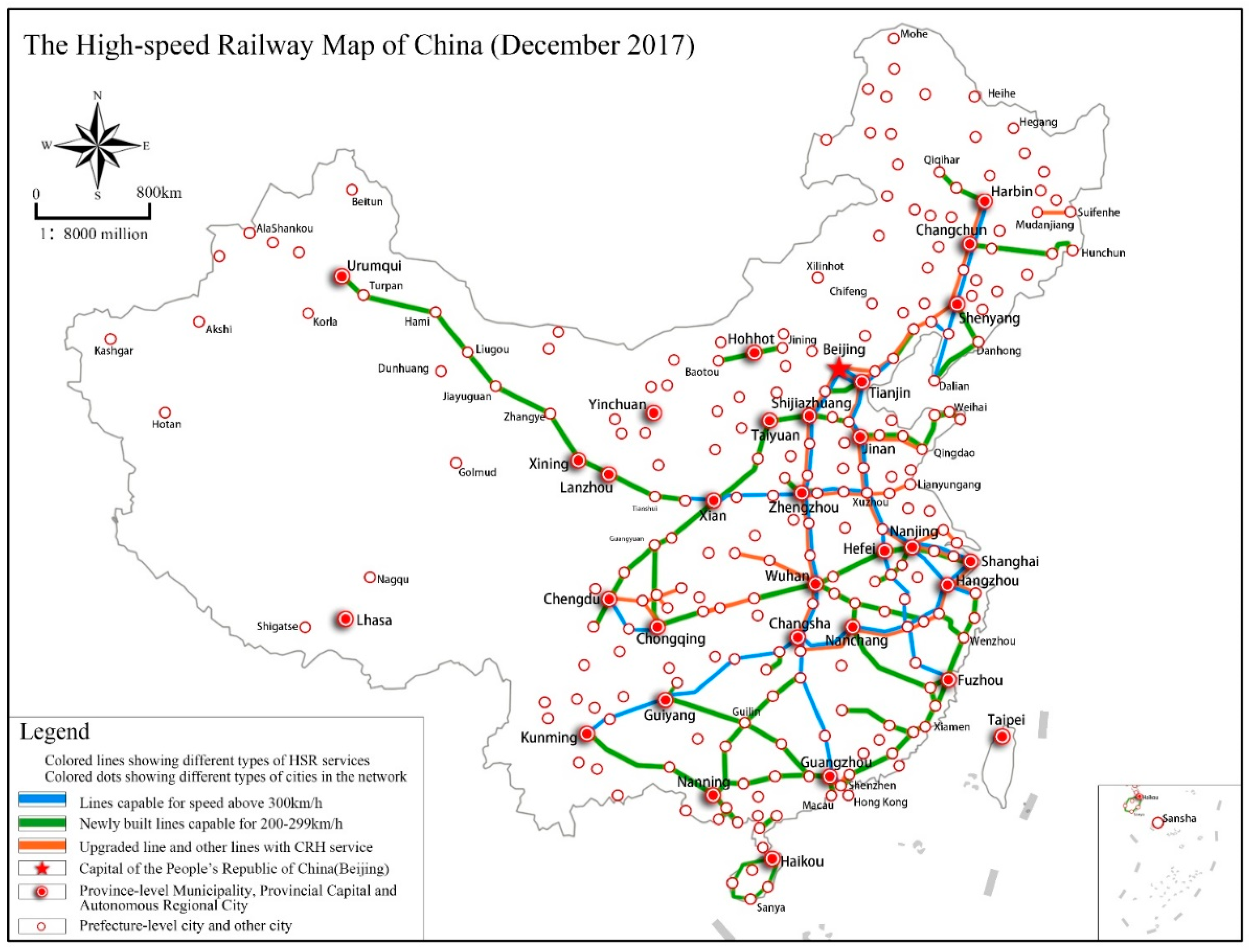
The existing HSR corridor maps of China with the cities it serves are presented in Figure 2. Figure A1 shows the planned HSR corridors that will connect all provinces of China except Tibet by 2025. Specifically, having sped up, promoted, and spread nationally between 2009 and 2016, China’s HSR network now serves all the prefecture-level cities, thereby presenting us with a representative case for investigating the relationship between HSR policy and city-level housing prices with special attention on regional disparity from a national perspective.

Whether or not China’s ambitious HSR plan can be beneficial for economic development depends not only on the growth of real output, but also on the confidence of the market in the sustainable growth of the Chinese economy [9]. The underlying principle is that housing prices can reflect the economic effect of the current period, and more importantly the confidence of the residents in future economic growth. Moreover, city-level housing price is one of the most important factors affecting the competition between cities, especially between megacities and small cities. In this regard, city-level housing price typically represents the future development potential of the city.

Although the impact of rail infrastructure on housing prices has been examined extensively, research findings have not been consistent. Some have found that the improvement of rail transport facilities has a positive effect on housing values [10,11,12,13,14], whereas others have found the impact is minor [15,16]. Moreover, most analyses have been focused on urban rail projects, whereas the studies with a particular focus on the impact of intercity transport mode (such as the HSR) on the intracity issue (such as the city-level housing price) have been quite limited. The HSR differs from conventional railways (such as commuter rail, light rail and metro) in terms of service market and distance. Since HSR normally serves as a premium ground transportation mode, patrons who use the system are much different from those who use conventional rail services, especially in China, where the price differences are very large relative to income [17]. In addition, unlike an urban transit system, HSR provides an intercity transport service, normally by connecting major metropolitan centers with a distance between 160 and 800 km [18]. Because of the advantage of speed, HSR binds housing and labor markets together to a commuting region [19], which may thus make commuting at a larger geographic scale become possible. Overall, since empirical research has been too limited so far, it is unclear whether there is any linkage between HSR development and the prosperity of the city-level real estate market nationwide in China.

This study was intended to meet that need by establishing a theoretical framework and developing a fixed-effect model with a comprehensive dataset. It expands the existing research perspective of infrastructure on economic development, provides a more in-depth discussion of the externality of infrastructure investment, which is calculated quantitatively in terms of the reflection of the real estate market, and intensifies the understanding of HSR over regional disparity. The study differs from previous works in a number of ways.

First, it offers a framework to serve as the general theoretical underpinning for the empirical study that follows, which further assesses the linkages between HSR development and disparity in terms of changes in city-level housing prices, thus helping to deeply understand the systematic and causal relationship between HSR and housing price.

Second, unlike existing studies on this issue that employed provincial data or selected a single HSR line within a certain region to carry out research, this study utilized a nationwide dataset that included 285 Chinese cities during the period from 2009 to 2017, during which two great revolutions of China’s HSR development were observed: In 2009, the Beijing–Tianjin Intercity Railway opened to traffic, which was China’s first HSR line with a speed of over 350 km per hour and fully independent intellectual property rights, and by the end of 2015, China had basically completed its “four north-south and four west-east corridors” national HSR network. Thereby, almost all the prefecture-level cities were connected to the existing HSR network, except Lhasa in the Xizang (Tibet) Autonomous Region. As a result, this study was able to investigate the impact of the HSR on city-level housing prices in different stages of the HSR implementation policy. Furthermore, our research divided all the selected cities into three grades and three kinds of pairs according to several relevant policies promulgated by the state so as to better understand the difference in the impact that the HSR had on city-level housing prices between various city groups and city pairs.

The empirical findings were as follows: (1) The introduction of HSR leads to a 13.9% increase in city-level housing prices, and the figures for national central cities and regional central cities were 31.7% and 19.6%, respectively; (2) regional imbalances were mitigated with the development of the HSR, and some central cities in underdeveloped regions were stimulated with regard to housing price growth; (3) siphon effects and diffusion effects were observed in megacity–small city pairs, whereas synergistic effects often lay in megacity–megacity pairs, and such effects all tended to be more significant with increases in the number of HSR lines and a drop in the travel time.

The rest of the paper is organized as follows: Section 2 presents a literature review. Section 3 illustrates a theoretical framework of HSR development increasing the housing price. Section 4 depicts the data, defines the variables, and presents summary statistics and methodology. Section 5 presents empirical results, and Section 6 summarizes and concludes.

2. Literature Review

The development of the HSR served as an important influencing factor, or a vital intermediate variable of decision-making on real estate investment. One fundamental question is whether the development of HSRs exerts a positive effect on housing price growth. For a long period of time, researchers have had very different views on this. For example, Andersson et al. [15] studied the effect of the western HSR line in Taiwan on housing values in cities along it. Their results indicated that HSR accessibility had at most a minor effect on house prices, whereas a negative price effect associated with this issue has also been found, probably due to higher levels of noise or crimes [20]. Amid such disagreements, the literature on the HSR and changes in housing prices continues to expand with both theoretical models and advanced empirical methods.

A variety of theoretical models have been proposed to analyze the connection between rail system and housing price growth. Zheng and Kahn [9] noted that the efficient markets theory of asset pricing posits that housing price reflects the expected present discounted value of future rents. The theory suggests that changes in city real estate price dynamics should reflect the expected impact of major infrastructure investments. Moreover, a housing unit can be seen as a complex good composed of an array of individual attributes. Given such considerations, the hedonic theory suggests that the scale price of such a complex good can be expressed as a function of the specific combination of its characteristics [21]. In theory, public transport infrastructure generates two opposite effects, positive externalities based on improved accessibility to urban amenities and negative, proximity externalities linked to nuisance due to noise, increased traffic, and criminality.

However, there is also vast empirical literature on the issue. Regardless of whether the research perspective was macro or micro, the majority of the existing studies have observed positive results. Most previous studies, although limited in a single region, a certain city, or a typical HSR line, have found positive property value impacts of rail transit systems, and many of them relied on the Ordinary Least Squares (OLS) method [22,23,24,25,26]. A handful of studies conducted in Asian cities, such as Bangkok, Thailand [27], Seoul, Korea [28], and Beijing, China [16], have found positive impacts on property values. A national-scale study also showed similar results, even though studies with similar dimensions were very few [9].

Some literatures focused on the impact of the HSR on housing prices, observing disparities both within and between cities. From an intracity perspective, some authors have suggested that the effect varies according to the characteristics of the stations and their location, types of rail mode, development stages, housing markets, and land-use characteristics [16,26]. From an intercity perspective, the impact may considerably vary among cities depending on the actual ridership level [29], and the type of clientele [23]. Bowes and Ihlanfeldt [23] suggesting that a good combination of transportation modes and the feasibility of multimodal trips can raise housing prices.

In sum, the linkage between HSR development and city-level housing prices involves complicated mechanisms that require careful consideration in the process of impact assessment. Although a positive link between rail system (or HSR) and housing price increase has been observed in most micro or macro cases, and a great amount of literature has partially studied the reason why disparities in the impact are significant both regionally and locally, the causal relationship between them has not been clearly addressed yet. Besides, studies of national scale have been very few, and their dataset has been limited in the length of time. Moreover, the city groups for most of the historical studies have been classified according to their geographic location (the east, the middle, the west), which is not reasonable for the rapid development of China’s HSR network. Hence, there are two problems to be solved: (1) What role does HSR play in the transmission mechanism from gathered factors to changes in housing prices? (2) How and to what extent does the HSR network in China affect city-level housing price?

For the first problem, we developed a theoretical framework (details in Section 3) based on a great deal of historical literature relevant to this issue. To answer the second question, we did an empirical study from a national research scale using data from 285 cities in China (details in Section 4 and Section 5) throughout 2009–2017, with just one HSR line at the beginning, and the existing national network, known as “the four north-south and four west-east HSR corridors”, which covered almost all the prefecture-level cities in China by the end of 2015.

3. How the HSR Affects City-Level Housing Prices: A Theoretical Framework

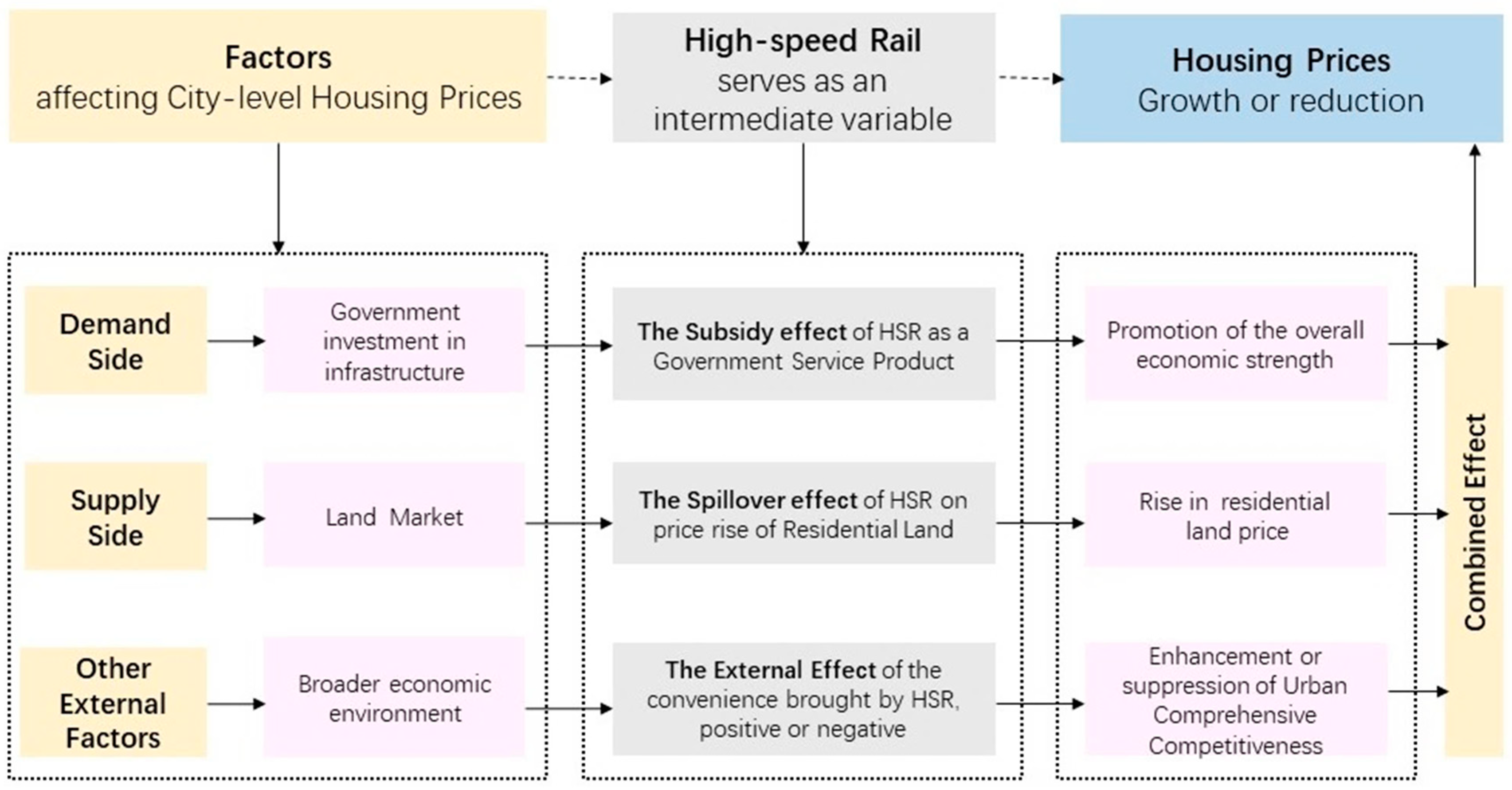
This paper is interested in the role that HSR development has played in the changes of the city-level housing prices. The conceptual framework for assessing the linkages between HSR development and disparity measured in terms of changes in city-level housing price is illustrated in Figure 3, which serves as a general theoretical underpinning for our empirical analysis. Note that the framework is also applicable to other modes of transportation. Although there are many variables that affect housing price, including population inflow, land supply, resource concentration, and others, transportation convenience becomes an important intermediate variable to facilitate the transformation from population and resource inflow, as well as economic growth to housing price increase. The operation of the HSR pushes a series of important variables to play a synergistic role, ultimately affecting housing price. Specifically, such a causal relationship can be analyzed from three dimensions: (1) The demand side, (2) the supply side, and (3) other external factors.

From the demand side, HSR is an important part of the urban infrastructure system and also a typical kind of public product provided by the government, and it plays the role of “subsidy effect” of government public goods. Evidence has confirmed that the construction of the HSR generated short-term impacts on accessibility and connectivity, and it inevitably has had long-term impacts on the relocation, agglomeration, and diffusion of economic activities [30,31]. Changes in connectivity caused by HSR lines played a more important role in economic development than in time saving [32]. HSR lines increased the connectivity of cities and mostly enlarged their market areas, so it was much easier for producers in peripheral cities to transport their products to core cities [33]. Government investment in HSR was not profitable in the short term, but it had a better economic environment, with the major cities showing strong increases in both population and employment, economic activities, and land values [34,35]. Therefore, it might have boosted their economic growth and ultimately catalyzed an increase in housing prices, and vice versa.

From the supply side, there is a transmission mechanism from land price to housing price with both direct and indirect perspectives. On the one hand, the government’s massive expropriation of land for public facilities (HSR) would competitively reduce the supply of residential land. On the other hand, after the introduction of the HSR, a city would further attract more construction of supporting infrastructure related to commercial, educational, or medical resources. Then, the rising demand for commercial land such as office buildings and factories would thereby squeeze the supply of residential land as well. As a consequence, the aggravated competition caused by the construction of the HSR in the land market could have a spillover effect on housing price [23].

In addition, there have been several other external reasons why the HSR has led to disparities with regard to changes in housing price between different cities. For instance, HSR has further reduced transaction costs and has improved efficiency by competing with other means of transportation, such as aviation [5,36] and highways [37]. Moreover, the HSR network enhanced the connection between metropolis and small cities, as well as central cities and satellite cities, leading it to become much more conducive in terms of the division of labor to further specialization, thus facilitating inter-regional and intra-regional resource allocation to be more efficient [38]. Furthermore, HSR has proven to increase residents’ duration of visit [39], releasing long-suppressed travel demand and thereby supporting housing prices in some tourist cities.

4. Variables, Data, and Methodology

This section defines variables and describes data. We used city-level data to examine the relationship between HSR development and housing price growth in China. To measure housing values, we made use of a number of financial variables and economic indicators.

4.1. Variables

Traditional indicators of housing prices have been employed by existing inner-city studies, such as city’s own population (POP), the market potential (MP) variable (defined as the distance weighted purchasing power of neighboring cities), and other inner-city factors affecting housing price growth, such as greenery, healthcare, education, highway, rail, and military [9,40]. This paper makes use of some financial indicators, such as saving and loans [41], to avoid the interference from financial bubbles on research results. On the one hand, real estate investment is greatly influenced by the supply of financial supply, and on the other hand, national macro policy control is generally by means of financial means, which can partly serve as government regulation. The definition and descriptive statistics of the variables are shown in

Table 1. Summary statistics (9 years, 285 cities, 2009–2017).

Symbols	Definition	Minimum	Maximum	Mean	SD	Observations
y	ln(housing price)	7.4697	10.9642	8.8197	0.4893	1042
hsr	HSR	0	1	0.2760	0.4471	2565
pop	Ln(population)	2.7147	7.8043	4.6103	0.7722	2565
air	Airline	0	1	0.4596	0.4985	2565
rail	Railway	0	1	0.9341	0.2481	2565
save	Savings/GDP	0.0430	4.1361	0.8454	0.3962	2515
loan	Loans/GDP	0.0623	84.6609	1.5597	2.2602	2516

Notes: SD = standard deviation. All the values were measured in millions of Renminbi (savings, loans, GDP), in tens of thousands (population, total permanent resident population), and with two dummy variables, airline and rail (1 represents available and 0 not). Source: Authors.

.

4.2. Samples and Data

According to Chinese government administrative classifications, there are three levels of cities in China: Municipalities, prefecture-level cities, and county-level cities. There are four municipalities: Beijing, Shanghai, Tianjin, and Chongqing, and all of them are governed directly by the central government and are not subject to the administration of any provincial government. Each province in China has about 10 prefecture-level cities, which are governed directly by the provincial government. A county-level city is usually governed by a prefecture-level city. In this paper, a “city” refers to either a prefecture-level city or a municipality.

The study area included all the prefecture-level cities and municipalities, limited to the mainland of China (excluding Hong Kong, Macao, and Taiwan). Thus, 285 cities were chosen as the objects for this study, and they could be divided into three types according to several “City Classification Criteria” officially announced by the state:

(1)

9 national central cities (abbreviated as N), including Beijing, Tianjin, Shanghai, Guangzhou, Chongqing, Chengdu, Wuhan, Zhengzhou, and Xi’an (according to the National Urban System Plan (2010–2020), China’s highest-level strategic plan, which was jointly prepared by 19 central ministries and commissions, including the Ministry of Housing, the National Development and Reform Commission, the Health and Family Planning Commission, and the Ministry of Education);

(2)

27 regional central cities (abbreviated as R), including all the provincial capital cities and Municipalities with Independent Planning Status under the National Social and Economic Development Plan (Shijiazhuang, Shenyang, Dalian, Changchun, Taiyuan, Hohhot, Harbin, Jinan, Qingdao, Nanjing, Hangzhou, Xiamen, Shenzhen, Suzhou, Ningbo, Hefei, Fuzhou, Nanchang, Changsha, Nanning, Haikou, Guiyang, Kunming, Lanzhou, Xining, Yinchuan, and Urumqi: These cities are provincial cities or “Municipalities with Independent Planning Status under the National Social and Economic Development Plan”, issued by the nation); and

(3)

249 other prefecture-level cities (abbreviated as O), and these are ordinary prefecture-level cities officially announced by China’s National Government.

We collected a set of panel data from 285 Chinese prefecture-level cities and municipalities over the period 2009–2017. The data source for the study comprised five parts:

(1)

Housing price data, a 2009–2017 dataset including 285 city-level real estate prices (the commercial housing transaction price) selected from “ANJUKE (https://anjuke.com)”, one of the largest real estate internet portals in China;

(2)

Railway and HSR data (whether or not a certain city possessed a railway or HSR, respectively) from “National Railway Passenger Train Schedules (2009–2017)”, provided by China’s railway customer service center (according to the definition of the National Railway Administration (2014), the HSR in China includes rail lines served by G-, C-, and D-prefixed bullet trains, but in our study, we only took newly constructed HSR lines into account served by G- and C-prefixed bullet trains and excluded HSR lines sped up on ordinary rail lines, served by D-prefix bullet trains);

(3)

Population data (total population of municipal districts was introduced to control for heterogeneous patterns of residential characteristics among different cities) sourced from “China’s City Statistical Yearbook (2009–2017)”;

(4)

Financial data, GDP, savings, and loans (total savings in municipal districts, total loans in municipal districts) collected from “China’s City Statistical Yearbook (2009–2017)”; and

(5)

Airport data (whether or not a certain city possessed an airport) extracted from “the official Civil Aviation Industry Development Statistics Bulletin (2009–2017)”, which are published on the website of the Civil Aviation Administration of China (CAAC). It was considered to be no airport when the following two situations occurred: (1) The airport was licensed for operating permission, but there were no flights opened yet, and (2) the airport shut down for a certain year for the reason of long-term maintenance.

Note that the HSR and rail data were collected at the beginning of the year, whereas others were gathered by the end of the year, and all the data for a year was treated as the same period in our study.

4.3. Methodology

This study used the operation of the high-speed rail in China as a natural experiment to test the effects of transport infrastructure networks on city-level housing price. We used a fixed effect model (FE) to get the baseline regression, and a Generalized method of moments (GMM) estimation of dynamic panel data model as a robustness check. We also developed a regression model with city classification dummies and regional dummies to further study the economic impact.

4.3.1. Baseline Regression: Fixed Effect Model

Our panel data analyses used data over the period 2009–2017 for 285 cities. To investigate the relationship between the high-speed railway and housing prices, our baseline regression model was:

$$y_{i,t}={\beta }_0+{\beta }_{1}hs{r}_{i,t}+{\beta }_{2}po{p}_{i,t}+{\beta }_{3}ai{r}_{i,t}+{\beta }_{4}rai{l}_{i,t}+{\beta }_{5}sav{e}_{i,t}+{\beta }_{6}loa{n}_{i,t}+{\mu }_i+{\epsilon }_{i,t},$$

(1)

where i indexes one of the 285 cities and t indexes one of the years, and the dependent variable y_i,t is the logarithm of urban average housing price. Our key variable, hsr_i,t, is the dummy variable, which represents whether the ith city had HSR in the panel data. An HSR operating in the city was hsr_i,t = 1, and otherwise, hsr_i,t = 0. The lag term, hsr_i,t−1, was included in the regression results to investigate the dynamic impact of HSR on housing price; pop_i,t, air_i,t, rail_i,t, save_i,t, and loan_i,t are control variables; pop_i,t represents the level of population; air_i,t represents whether the city owned an airport or not; rail_i,t represents whether the city owned an ordinary railway or not; save_i,t and loan_i,t represent the financial development of the city; u_i is unobserved city-specific fixed effects; and ε_i,t is an idiosyncratic error term.

A fixed effect model was adopted to estimate the baseline regression, with the assumption that the population being sampled was normally irregularly-distributed, as a common variance and additive error structure is often violated in OLS analysis. The Hausman specification test was conducted to test for orthogonality of the common effects and the regressors, assessing whether a fixed effect model was preferred to a random effect model. A least squares dummy variable (LSDV) approach was used to estimate the baseline regression, which included all the city’s dummy variables using the first city, Beijing, as a benchmark city. To address the time-lagged effect of HSR on housing price, the first lagged value of the dummy variable hsr_i,t−1 was included in the baseline regression as a substitute variable of current value.

4.3.2. Dynamic Panel Data Model

The efficient markets theory of asset pricing posits that real estate prices reflect the expected present discounted value of future rents. This theory suggests that changes in city real estate price dynamics should reflect the expected impact of major infrastructure investments [9]. Considering the dynamic process of housing prices, we developed a dynamic panel data model:

$$y_{i,t}={\beta }_0+{\beta }_1{y}_{i,t-1}+{\beta }_{2}hs{r}_{i,t-1}+{\beta }_{3}hs{r}_{i,t}+{\beta }_{4}po{p}_{i,t}+{\beta }_{5}ai{r}_{i,t}+{\beta }_{6}rai{l}_{i,t}+{\beta }_{7}sav{e}_{i,t}+{\beta }_{8}loa{n}_{i,t}+{\mu }_i+{\epsilon }_{i,t}$$

(2)

where the set of right-hand-side variables includes the lagged dependent variable y_i,t−1, which includes the entire history of the right-hand-side variables in the equation, so that any measured influence is conditioned on this history. In the dynamic panel data model, the correlation between the lagged dependent variable y_i,t−1 and the compound disturbance u_i + ε_i,t makes the LSDV estimators for panel data inconsistent even if ε_i,t is not serially correlated, since the same u_i enters the equation for observation in group i. We then estimated Equation (2) using the difference-GMM approach (Arellano and Bond, 1991) as well as the system-GMM approach (Arellano and Bover, 1995; Blundell and Bond, 1998).

Two specification tests suggested by Arellano and Bond [42], Arellano and Bover [43], and Blundell and Bond [44] were carried out: (1) The first was the Sargan test for overidentification restrictions, which tests the overall validity of the instruments, where under the null hypothesis that the instruments are valid, the test statistic is asymptotically distributed as a chi-square with the degree of freedom being equal to the number of instruments minus the number of parameters estimated; (2) and the second was the second-order serial correlation test, which examines the hypothesis that the error term ε_i,t is not serially correlated. Under the null of no second-order serial correlation, the test statistic is asymptotically distributed as standard normal.

4.3.3. Regression Model with City Classification Dummies and Regional Dummies

Chinese cities were divided into three types according to several City Classification Criteria officially announced by the state. There were 9 national central cities, 27 regional central cities, and 249 other prefecture-level cities. We introduced city classification dummy variables and cross terms to study the heterogeneity of different classification cites. The regression model with city classification dummies was

$$y_{i,t}={\beta }_0+{\beta }_{1}hs{r}_{i,t}+{\beta }_{2}hs{r}_{i,t}\ast N_i+{\beta }_{3}hs{r}_{i,t}\ast R_i+{\beta }_4{N}_i+{\beta }_5{R}_i+{\beta }_6{x}_{i,t}+{\mu }_i+{\epsilon }_{i,t}$$

(3)

where N_i and R_i are city classification dummy variables. When the city was a national central city, N_i = 1, and otherwise, N_i =0. When the city was a regional central city, R_i = 1, and otherwise, R_i = 0. The vector x_i,t is a set of control variables used in Equation (1).

Hence, we could rewrite the regression model for national central cities, regional central cities, and other prefecture-level cities in Equations (4)–(6):

$$y_{i,t}=({\beta }_0+{\beta }_4)+({\beta }_1+{\beta }_2)hs{r}_{i,t}+{\beta }_6{x}_{i,t}+{\mu }_i+{\epsilon }_{i,t},N_i=1,$$

(4)

$$y_{i,t}=({\beta }_0+{\beta }_5)+({\beta }_1+{\beta }_3)hs{r}_{i,t}+{\beta }_6{x}_{i,t}+{\mu }_i+{\epsilon }_{i,t},R_i=1,$$

(5)

$$y_{i,t}={\beta }_0+{\beta }_{1}hs{r}_{i,t}+{\beta }_6{x}_{i,t}+{\mu }_i+{\epsilon }_{i,t},N_i=0,R_i=0.$$

(6)

According to the level of economic development, China’s provinces could be defined as eastern, central, and western regions. The eastern provinces covered Beijing, Tianjin, Hebei, Liaoning, Shanghai, Jiangsu, Zhejiang, Fujian, Shandong, Guangdong, Guangxi, and Hainan. The central provinces covered Shanxi, Inner Mongolia, Jilin, Heilongjiang, Anhui, Jiangxi, Henan, Hubei, and Hunan. The western provinces covered Chongqing, Sichuan, Guizhou, Yunnan, Shaanxi, Gansu, Qinghai, Ningxia, and Xinjiang. We used a similar strategy to introduce regional dummies into our regression model, and thus the definitions East_i and Central_i were regional dummies for cities. When the city was an eastern city, East_i = 1, and otherwise, East_i = 0. When the city was a central city, Central_i = 1, and otherwise, Central_i = 0.

5. Empirical Results

5.1. Results of Baseline Regression and Dynamic Panel Data Model

The results from the baseline estimations are summarized in

Table 2. Housing price and HSR: Baseline and Generalized method of moments (GMM) Regressions.

	Baseline Regression: Fixed Effect Model		Dynamic Panel Data Model
			Difference GMM	System GMM
hsri,t−1	0.139 ***		0.048 *	0.073 ***
	(0.204)		(0.025)	(0.024)
hsri,t		0.185 ***	0.072 **	0.086 **
		(0.022)	(0.036)	(0.036)
yi,t−1			0.670 ***	0.805 ***
			(0.056)	(0.036)
pop	0.382 ***	0.491 ***	0.361 ***	0.185 ***
	(0.051)	(0.053)	(0.070)	(0.053)
air	−0.018	−0.021	0.065	−0.038
	(0.060)	(0.066)	(0.053)	(0.119)
rail	0.033	0.027	−0.171 **	−0.220 ***
	(0.140)	(0.154)	(0.070)	(0.083)
save	−0.058	−0.064	0.234 ***	0.238 ***
	(0.053)	(0.056)	(0.076)	(0.079)
loan	0.049 ***	0.070 ***	0.016 **	−0.003
	(0.010)	(0.010)	(0.009)	(0.011)
constant	6.803 ***	6.189 ***	1.027 **	0.864 **
	(0.301)	(0.320)	(0.478)	(0.341)
Observations	1000	1031	532	779
Diagnosis	R2 = 0.3397 Hausman test (p = 0.00)	R2 = 0.3260 Hausman test (p = 0.00)	Sargan test (p = 0.00) First-order (p = 0.00) Second-order (p = 0.38)	Sargan test (p = 0.00) First-order (p = 0.00) Second-order (p = 0.28)

Notes: Cities in Tibet were excluded from the sample due to missing data. The standard errors are in parentheses; *** the significance levels are at 1%; ** the significance levels are at 5%; * the significance levels are at 10%.

and suggested that HSR exerted a significant positive impact on city-level housing prices, and that the extent of the impact for hsr_t was larger than that for hsr_t−1, which can be explained by the following two major reasons. First, there was probably a psychological expectation that housing prices would grow before an HSR line was officially announced to be constructed in the city. Besides, the sale of China’s commercial residential housing generally adopts the pre-sale system, stimulating housing prices before the operation of the HSR. We also investigated the results of hsr_t−n, and the coefficient of hsr_t−n was not significant. One of the underlying reasons could be that inconvenient public services, facilities, and infrastructures were not available when the HSR line was newly put into service, and also another reason was that real estate system often takes one year for pre-sale.

Considering the dynamic process of housing prices, an alternative estimation was by use of the GMM approach through the dynamic panel data estimation. One advantage of the GMM approach was that it helped reduce the problem of multicollinearity among the explanatory variables and endogeneity between the dependent and explanatory variables. The results of first-differenced GMM and the system GMM estimations are displayed in Table 2, comparatively. Our results, that the introduction of HSR increased the city-level housing price, were robust when including both the lagged dependent variable y_i,t−1 and the lagged independent variable hsr_i,t−1 in the dynamic panel data model.

To be more specific, HSR, population, and financial development had significant positive impacts on housing prices in the baseline regression, which suggests that housing prices in our sample cities in the HSR network were primarily driven by demand and improved infrastructure. From the first-differenced GMM estimations and the system GMM estimations, similar and positive impacts could be considerably observed among HSR, population, and financial development, while varying in degree. For instance, from the baseline regressions in Table 2, HSR served as a vital variable in the intercity context when assessing the changes in housing prices, and it stimulated housing prices growth by 13.9%.

5.2. Results of City Classification Dummies and Regional Dummies (National-Scale)

5.2.1. Impacts Varied between Different City Dummies

The result of the impact distribution in different city hierarchies are shown in

Table 3. Housing price and HSR with city classification dummies.

	Pooled Data		Panel Data: Fixed Effect Model
	Beta	Standard Errors	Beta	Standard Errors
hsr	−0.003	0.028	0.049	0.033
hsr*N	0.600 ***	0.078	0.317 ***	0.056
hsr*R	0.349 ***	0.061	0.196 ***	0.048
N	0.087 *	0.077
R	0.102 **	0.048
pop	0.122 ***	0.021	0.482 ***	0.052
air	0.083 ***	0.027	−0.017	0.065
rail	0.040	0.082	0.023	0.150
save	−0.171 ***	0.033	−0.043	0.055
loan	0.086 ***	0.014	0.061 ***	0.010
constant	8.049 ***	0.129	6.256 ***	0.313
Observations	1031		1031
Diagnosis	R2 = 0.4632		R2 = 0.3735 Hausman test (p = 0.00)

Notes: Cities in Tibet were excluded from the sample due to missing data; *** the significance levels are at 1%; ** the significance levels are at 5%; * the significance levels are at 10%.

, and we made a comparison between pooled data and panel data. With regard to the impact that HSR had on city-level housing prices, disparities were found between cities of different hierarchies, consistent with several former studies [9,15]. The average effect in national central cities (N, large cities) was found to be much stronger than regional central cities (R, medium cities) and other prefecture-level cities (O, small cities). Statistically, the impact of HSR on housing prices was significant both in national central cities and regional central cities, whereas no visible relationship could be observed in small cities.

In the pool model, we could use the dummy variables N and R as explanatory variables, whereas in the FE model, the introduction of the dummy variables for each city was a perfect multicollinearity problem between city dummy variables and city classification dummy variables, so the N and R dummy variables, which represented the city class, were excluded in the FE model. In Table 2, The introduction of HSR leads to a 13.9% increase in city-level housing prices. However, in Table 3, the percentage of the impact in national central cities and regional central cities was 31.7% and 19.6%, respectively. In terms of other attributes, again, both the coefficient of population and financial development were statistically significant, whereas the coefficients of the railway and airport were not significant.

5.2.2. The Regional Imbalance Narrowed

Moreover, for the reason of sharing similar regional environments and location characteristics, the operation of HSR was expected to have both a direct effect on and an interrelationship with housing prices. The results of the impact between different regions are also shown in

Table 4. Housing price and HSR with regional dummies.

	Pooled Data		Panel Data: Fixed Effect Model
	Beta	Standard Errors	Beta	Standard Errors
hsr	0.021	0.063	0.145 ***	0.048
hsr*East	0.135 **	0.070	0.064	0.056
hsr*Central	0.014	0.073	0.025	0.064
East	0.336 ***	0.039
Central	0.089 **	0.043
pop	0.211 ***	0.016	0.485 ***	0.053
air	0.140 ***	0.026	−0.021	0.066
rail	−0.036	0.082	0.030	0.154
save	−0.117 ***	0.032	−0.069	0.056
loan	0.090 ***	0.012	0.070 ***	0.010
constant	7.419 ***	0.110	6.214 ***	0.321
Observations	1031		1031
Diagnosis	R2 = 0.4791		R2 = 0.3373 Hausman test (p = 0.00)

Notes: Cities in Tibet were excluded from the sample due to missing data; *** the significance levels are at 1%; ** the significance levels are at 5%; * the significance levels are at 10%.

, regressed with pooled data and panel data separately. The results show that city-level housing prices were gradually decreasing from the east to the west in the pooled data model, which means that there were disparities between regions to a certain extent. However, with the introduction of HSR, the regional gap shrunk. Statistically, the evidence is that the coefficients of hsr*east and hsr*central were not significant, whereas the figure for hsr, representing the western region, was 0.145 and significant at the 1% level in the fixed effect model.

The other interesting finding from Table 4 was that our finding was completely opposite to that of Sun and Yuri [45]. HSR promoted the development of some national and regional central cities in the relatively underdeveloped central and western regions of China in terms of a rise in housing prices. These key cities were represented by Chongqing, Chengdu, Xi’an, Zhengzhou, and Wuhan in the existing network. Such HSR hub cities often have a large economy scale and a number of amenities, entertainment, educational and medical resources, infrastructure, and service facilities of comparatively higher quality, thus attracting people from the surrounding small cities or rural areas, as previous studies have shown [35], and consequently increasing the final demand of the sectors in the cities, such as housing demand.

5.3. Subsample Estimations with More Inner-City Explanatory Variables (35 Key Cities)

The baseline research on 285 cities may have had some limitations. First, a large number of small cities only opened an HSR in recent years, so we could not observe the long-term effects. Second, the housing price data for small cities in earlier years were not provided on the website (ANJUKE, https://anjuke.com). Third, factors such as policies of limited purchase, land use, the subway, and others are all important in a city-level housing price study, but it is difficult to obtain such sufficient data in small cities. Thus, in this section, we developed a more detailed study on 35 key cities that introduced the HSR as the first group, and the data were more official and detailed. The definition and descriptive statistics of variables for the subsample estimations are shown in

Table 5. Summary statistics (9 years, 35 cities, 2008–2016).

Symbols	Definition	Minimum	Maximum	Mean	SD	Observations
y	Housing price (in logs)	7.8284	10.7254	8.8189	0.5057	315
hsr	HSR	0	1	0.5302	0.4999	315
pop	Population (in logs)	5.8497	7.8034	4.4868	0.6756	315
restr	Restriction	0	1	0.3841	0.4872	315
metro	Metro	0	18	1.7683	3.4104	315
rail	Railway	0	1	0.9968	0.0563	315
save	Savings/GDP	0.0787	1.995	0.8613	0.2545	305
loan	Loans/GDP	0.0623	4.6291	0.7000	2.2402	304
land	Residential Land/construction land	0.1887	0.7143	0.3079	0.073	262

Notes: SD = standard deviation. All the values were measured in municipal districts in millions of RMB (GDP, savings, loans), in tens of thousands (population), and with three dummy variables (restriction, airline, rail and restriction policy) (1 represents available and 0 not). Sources: housing prices from China’s State Statistical Bureau; metro from the Mass Transit Group Portal of every city; restriction policy from the Portal of Municipal governments; land from the China Urban Statistics Yearbook.

. Note that the airport explanatory variable was dropped as a result of all the selected key cities having airports.

The results for the subsample estimations are in

Table 6. Housing price and HSR: Robust test using a fixed effect (FE) model (9 years, 35 cities, 2008–2016).

	(1)		(2)		(3)
	Beta	Standard Errors	Beta	Standard Errors	Beta	Standard Errors
hsri,t	0.207 ***	0.026	0.147 ***	0.024	0.142 ***	0.026
restri,t			0.017	0.018
restri,t+1					−0.039 **	0.019
pop	0.840 ***	0.100	0.501 ***	0.098	0.505 ***	0.114
metro			0.076 ***	0.010	0.060 ***	0.011
rail	0.000	0.171	−0.047	0.142	−0.030	0.137
save	−0.194 **	0.076	−0.255 ***	0.081	−0.208 **	0.082
loan	0.203 ***	0.026	0.136 ***	0.031	0.131 ***	0.034
land			0.100	0.326	−0.110	0.019
constant	3.511 ***	0.640	5.648 ***	0.634	5.686 ***	0.734
Observations	304 R2 = 0.5785 Hausman test (p = 0.00)		256 R2 = 0.5888 Hausman test (p = 0.00)		226 R2 = 0.5251 Hausman test (p = 0.00)
Diagnosis

Notes: The standard errors are in parentheses; *** the significance levels are at 1%; ** the significance levels are at 5%; * the significance levels are at 10%.

, which were similar with the baseline regression results in Table 3. Significantly, the introduction of HSR led to 20.7% for city-level housing price growth. Moreover, purchasing restriction policies did not work immediately on housing prices, which may have been the result of the long interval in our statistical investigation, while such policies can reduce and stabilize housing prices to a certain extent within one year. Furthermore, the introduction of a new subway can boost the housing prices, but such an impact was even smaller than that of the HSR has on the city-level housing prices.

5.4. Impacts Varied between Different City Pairs (Micro-Scale)

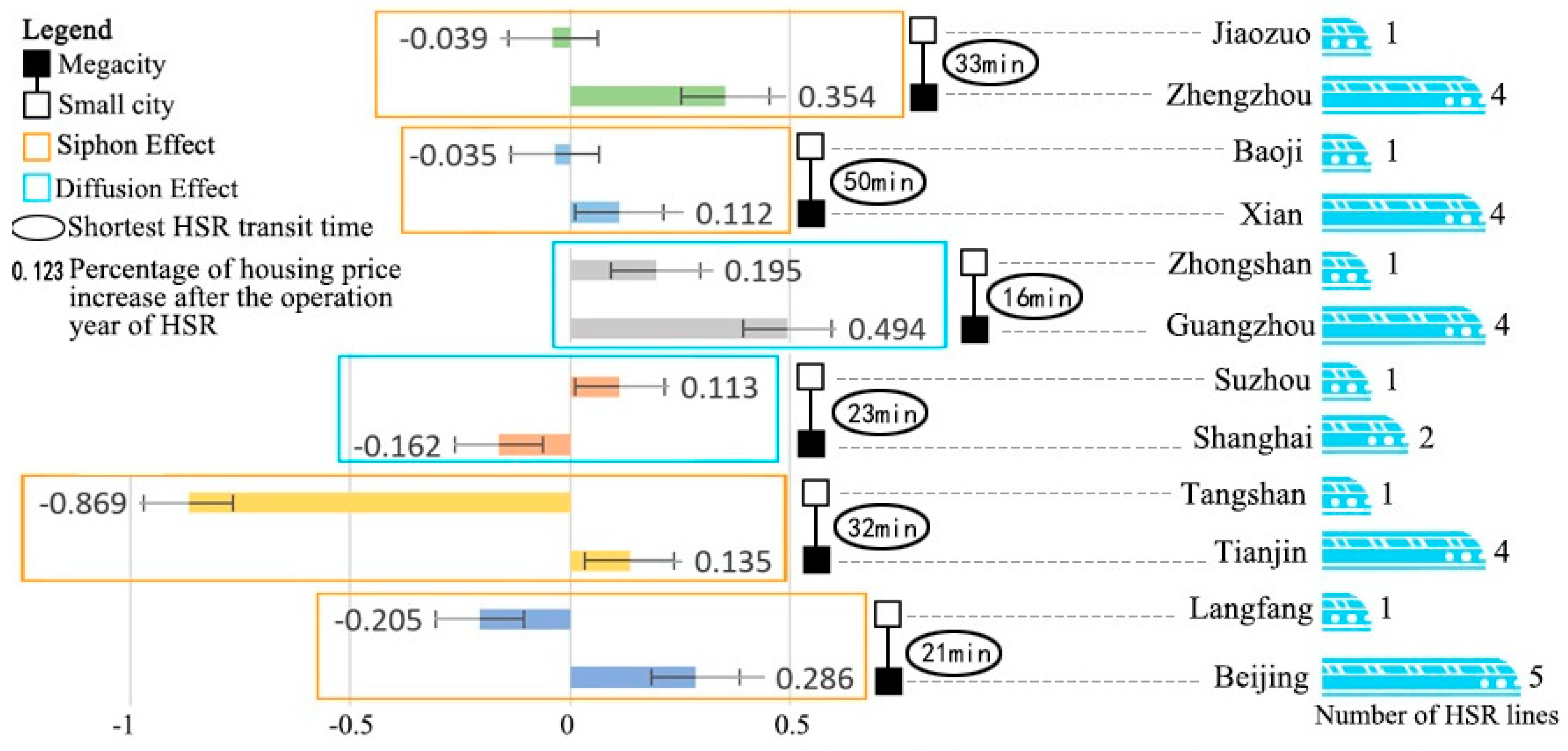
As already reviewed in Section 3, the HSR network could strengthen the connection between metropolis and small cities, as well as central cities and satellite cities, leading it to become much more conducive in terms of the division of labor with further specialization, thus facilitating inter-regional and intra-regional resource allocation to be more efficient (Pol, 2003; De Rus, 2008). In this section, in order to further understand the temporal and spatial distributions of the effect that HSR had on city-level housing prices, we made use of more intracity variables, such as the number of HSR lines passing through the city (Wang et al., 2017), and intercity variables, such as urban scale (Begoña et al., 2018) and least travel time between selected typical city pairs (as used in Zhu. et al, 2017), and studied from a micro scale to reinforce the former research.

There are three kinds of economic effects: The siphon effect (also called the trickle-down effect), the diffusion effect, and the synergistic effect. According to Myrdal G. (1971), the siphon effect means that the places and regions where economic activity is expanding will attract net population inflow, capital inflow, and trade activities from other regions, thus accelerating their own development and reducing the development speed of their surrounding areas. The diffusion effect means that all areas located around the center of economic expansion will receive capital and talent from the central region, and will be stimulated to promote the development of the region: As the infrastructure in the expansion center area improves, it gradually catches up with the central area. Myers (1993) indicated that the synergistic effect constitutes the compounded impact of two or more processes interacting in such a manner that their product is greater than the sum of their separate effects. Our results show that economic effects varied between different city-pairs: The siphon effect and the diffusion effect were observed in megacity–small city pairs, whereas the synergistic effect often lay in megacity–megacity pairs, and such effects all tended to be more significant with increases in the number of HSR lines and a drop in the travel time.

5.4.1. Impacts between Megacity and Small City Pairs

This type of city group is a difference in city scale, and travel times are small between them (about 30 min). As shown in Figure 4, the siphon effect (signaled by the yellow rectangles) and the diffusion effect (signaled by the blue rectangles) were observed in such city pairs, and the extent of economic characteristics came to be more considerable when the number of HSR lines of a megacity went up. With regard to the spatial distribution pattern, the siphon effect occurred in the north and inland hinterlands, such as in the city pair of Jiaozuo and Zhengzhou, Baoji and Xian, Tangshan and Tianjin, Beijing and Langfang, and the shorter the time distance between cities, the more significant the siphon effect was. Comparatively, the diffusion effect was observed in the southeastern coastal area, such as in Shanghai and Suzhou, Zhongshan and Guangzhou, and such an economic phenomenon tended to be more significant when travel time decreased.

5.4.2. Impacts between Megacity (or Central City) Pairs

This type of city group was similar in city scale, whereas travel time between them was comparatively longer than the previous group, generally between 1 h and 1.5 h. Figure 5 illustrates the impact between such city pairs. A synergistic effect, or economic integration (signaled by the purple rectangles), were observed in such pairs, whereas there was no obvious difference between the north and the south. It was interesting to find that the synergistic effect tended to be more conspicuous when travel time descended, such as Nanjing and Hefei, and when the difference between the number of lines in the two HSR hub cities went down. However, the simultaneous fall in housing prices in the pair of Dalian and Shenyang, in northeast China, may have been due to siphons from other major HSR hubs, such as Beijing and Tianjin, or to the weak economy of the two cities themselves.

6. Conclusions

During recent years, real estate values in China have experienced exponential growth and have attracted a lot of attention both from the public and the government. Even allowing for the increase in demand, housing speculation is generally regarded as a major attribute, but the improvement of transportation infrastructure such as the HSR may also play a role. The purpose of our study was to empirically investigate whether and to what extent did the HSR development affect the city-level housing prices in China, which provided a more in-depth discussion of the externality of infrastructure investment, which was calculated quantitatively in terms of the reflection of the real estate market.

This study was carried out with the aid of a dataset containing information both on HSR and housing prices, as well as financial, population, and transport variables for 285 Chinese municipalities and prefecture-level cities during 2009–2017. This study used the operation of the HSR in China as a natural experiment to test the effects of the HSR network on city-level housing prices, and then employed an FE model to get the baseline regression and GMM estimation of dynamic panel data models as robustness checks. To assess the city disparities and regional imbalance, city classification dummies and regional dummies were included in our econometric regression. Economic effects such as the siphon effect, diffusion effect, and synergistic effect were also studied with typical city pairs.

This study had three main findings: First, The introduction of HSR leads to a 13.9% increase in city-level housing prices, and the figures for national central cities and regional central cities were 31.7% and 19.6%, respectively. Second, regional imbalance was mitigated with the development of the HSR, and some central cities in underdeveloped regions were stimulated with regard to housing price growth. Third, the siphon effect and diffusion effect were observed in megacity–small city pairs, whereas the synergistic effect often lay in megacity–megacity pairs, and such effects all tended to be more significant with an increase in the number of HSR lines and a drop in the travel time.

However, even though the results could offer some insights for researchers into the space-time economic law in China and other countries in terms of the economic impact that the HSR has on housing prices, it is still worth noting that China’s unique political structure is likely to allow it to implement megaprojects efficiently. Chinese governments have strong power in supplying state-owned land, spending public money, and ignoring the possibly negative effects (such as noise) of HSRs on nearby residents. The other thing one should note is that the research findings were subjected to specific selected data samples and only reflected the case of the newly constructed HSR lines, served by G- and C-prefix bullet trains between 2009–2017. In further research, more detailed proxy variables will be included, such as intercity factors, including the spatial distance between cities, the number of passengers traveling via HSR, HSR volume, and intracity factors such as the number of HSR stations and the distance from stations to the city center. Moreover, other variables affecting housing prices, such as green rate and educational and medical variables, are also worth being considered.

References

- Jian, T.; Sachs, J.D.; Warner, A.M. Trends in regional inequality in China. China Econ. Rev. 1996, 7. [Google Scholar] [CrossRef]
- Zhang, Q.; Zou, H.F. Regional inequality in contemporary China. Ann. Econ. Financ. 2012, 13, 113–137. [Google Scholar]
- Chen, Z.; Haynes, K. Chinese Railway in the Era of High-Speed; Emerald Group Publishing Limited: Bingley, UK, 2015. [Google Scholar]
- Wu, Y.; Chen, Y.; Deng, X.; Hui, E.C.M. Development of Characteristic towns in China. Habitat Int. 2017, 77, 21–31. [Google Scholar] [CrossRef]
- Wang, K.; Xia, W.; Zhang, A. Should further expand its high-speed rail network? Consider the low-cost carrier factor. Transp. Res. Part A 2017, 100, 105–120. [Google Scholar] [CrossRef]
- Zheng, S.; Saiz, A. Introduction to the special issue “China’s urbanization and housing market”. J. Hous. Econ. 2016, 33, 1–3. [Google Scholar] [CrossRef]
- Cao, J.; Liu, X.C.; Wang, Y.; Li, Q. Accessibility impacts of China’s high-speed rail network. J. Transp. Geogr. 2013, 28, 12–21. [Google Scholar] [CrossRef]
- Jiao, J.; Wang, J.; Jin, F. Impacts of the high-speed rail lines on the city network in China. J. Transp. Geogr. 2017, 60, 257–266. [Google Scholar] [CrossRef]
- Zheng, S.; Kahn, M.E. China’s bullet trains facilitate market integration and mitigate the cost of megacity growth. Proc. Natl. Acad. Sci. USA 2013, 110, 1248–1253. [Google Scholar] [CrossRef]
- Bajic, V. The effects of a new subway line on housing prices in metropolitan Toronto. Urban Study 1983, 20, 147–158. [Google Scholar] [CrossRef]
- Knaap, G.J.; Ding, C.; Hopkins, L.D. Do plans matter? The effects of light rail plans on land values in station areas. J. Plan. Educ. Res. 2001, 21, 32–39. [Google Scholar] [CrossRef]
- Debrezion, G.; Pels, E.; Rietveld, P. The impact of railway stations on residential and commercial property value: A meta-analysis. J. Real Estate Financ. Econ. 2007, 35, 161–180. [Google Scholar] [CrossRef]
- Debrezion, G.; Pels, E.; Rietveld, P. The impact of rail transport on real estate prices an empirical analysis of the Dutch housing market. Urban Study 2011, 48, 997–1015. [Google Scholar] [CrossRef]
- Duncan, M. The impact of transit-oriented development on housing prices in San Diego, CA. Urban Study 2011, 48, 101–127. [Google Scholar] [CrossRef]
- Andersson, D.E.; Shyr, O.F.; Fu, J. Does high-speed rail accessibility influence residential property prices? Hedonic estimate from southern Taiwan. J. Transp. Geogr. 2010, 18, 166–174. [Google Scholar] [CrossRef]
- Zhang, M.; Meng, X.; Wang, L.; Xu, T. Transit development shaping urbanization: Evidence from the housing market in Beijing. Habitat Int. 2014, 44, 545–554. [Google Scholar] [CrossRef]
- Zhao, S.; Wu, N.; Wang, X. Impact of Feeder Accessibility on High-Speed Rail Share: Wuhan-Guangzhou Corridor, China. J. Urban Plan. Dev. 2018, 144, 04018029. [Google Scholar] [CrossRef]
- Button, K. Is there any economic justification for high-speed railways in the United States? J. Transp. Geogr. 2012, 22, 300–302. [Google Scholar] [CrossRef]
- Blum, U.; Haynes, K.E.; Karlsson, C. Introduction to the special issue: The regional and urban effects of high-speed trains. Ann. Reg. Sci. 1997, 31, 1–20. [Google Scholar] [CrossRef]
- Armstrong, R.J.; Rodriguez, D.A. An evaluation of the accessibility benefits of commuter rail in eastern Massachusetts using spatial hedonic price functions. Transportation 2006, 33, 21–43. [Google Scholar] [CrossRef]
- Rosen, S. Hedonic prices and implicit markets: Product differentiation in pure competition. J. Polit. Econ. 1974, 82, 34–55. [Google Scholar] [CrossRef]
- Billings, S.B. Estimating the value of a new transit option. Reg. Sci. Urban Econ. 2011, 41, 525–536. [Google Scholar]
- Bowes, D.R.; Ihlanfeldt, K.R. Identifying the impacts of rail transit stations on residential property values. J. Urban Econ. 2001, 50, 1–25. [Google Scholar] [CrossRef]
- Duncan, M. Comparing rail transit capitalization benefits for single-family and condominium units in San Diego, California. Transp. Res. Rec. 2008, 2067, 120–130. [Google Scholar] [CrossRef]
- Hess, D.B.; Almeida, T.M. Impact of proximity to light rail rapid transit on station-area property values in Buffalo, New York. Urban Study 2007, 44, 1041–1068. [Google Scholar] [CrossRef]
- Yan, S.; Delmelle, E.; Duncan, M. The impact of a new light rail system on single-family property values in Charlotte, North Carolina. J. Transp. Land Use 2012, 5, 60–67. [Google Scholar]
- Chalermpong, S. Rail transit and residential land use in developing countries: Hedonic study of residential property prices in Bangkok, Thailand. Transp. Res. Record 2007, 2038, 111–119. [Google Scholar] [CrossRef]
- Cervero, R.; Kang, C.D. Bus rapid transit impacts on land uses and land values in Seoul, Korea. Transp. Policy 2011, 18, 102–116. [Google Scholar] [CrossRef] [Green Version]
- Cervero, R.; Duncan, M. Neighbourhood Composition and Residential Land Prices: Does Exclusion Raise or Lower Values? Urban Stud. 2004, 41, 299–315. [Google Scholar] [CrossRef]
- Chen, C.L.; Hall, P. The impact of high-speed trains on British economic geography: A study of the UK’s 125/225 and its effects. J. Transp. Geogr. 2011, 19, 689–704. [Google Scholar] [CrossRef]
- Ureña, J.M.; Menerault, P.; Garmendia, M. The high-speed rail challenge for big intermediate cities: A national, regional, and local perspective. Cities. 2009, 26, 266–279. [Google Scholar] [CrossRef]
- Dupuy, G. Lurbanissme des Reséaux: Theotiésetmétgodes; Armand Collin: Paris, France, 1991. [Google Scholar]
- Spiekermann, K.; Wegener, M. Accessibility and spatial development in Europe. Sci. Reg. 2006, 5, 15–46. [Google Scholar]
- Sasaki, K.; Ohashi, T.; Ando, A. High-speed rail transit impact on regional systems: Does the Shinkansen contribute to dispersion? Ann. Reg. Sci. 1997, 31, 77–98. [Google Scholar] [CrossRef]
- Albalate, D.; Bel, G. The Economics and Politics of High-Speed Rail: Lessons from Experiences Abroad; Rowman and Littlefield Publishers: Lanham, MD, USA, 2012. [Google Scholar]
- Chen, Z.; Haynes, K. Impact of high-speed rail on regional economic disparity in China. J. Transp. Geogr. 2017, 65, 80–91. [Google Scholar] [CrossRef]
- Raturi, V.; Verma, A. Analyzing competition between High Speed Rail and Bus mode using market entry game analysis. Sci. Direct 2017, 25, 2373–2384. [Google Scholar] [CrossRef]
- Pol, P. The Economic Impact of the High-Speed Train on Urban Regions. In Proceedings of the 43rd European Regional Science Association ERSA Congress, Jyväskylä, Finland, 27–30 August 2003. [Google Scholar]
- Armando, C.; Luigi, P.; Ilaria, H. Hedonic value of high-speed services: Quantitative analysis of the students’ domestic tourist attractiveness of the main Italian cities. J. Transp. Res. Part A 2017, 100, 348–365. [Google Scholar]
- Lin, Y. Travel costs and urban specialization patterns: Evidence from China’s high speed railway system. J. Urban Econ. 2017, 98, 98–123. [Google Scholar] [CrossRef]
- Zhang, J.; Wang, L.; Wang, S. Financial development and economic growth: Recent evidence from China. J. Comp. Econ. 2012, 40, 393–412. [Google Scholar] [CrossRef]
- Arellano, M.; Bond, S. Some tests of specification for panel data: Monte Carlo evidence and an application to employment equations. The Review of Economic Studies. 1991, 58, 277–297. [Google Scholar] [CrossRef]
- Arellano, M.; Bover, O. Another look at the instrumental variable estimation of error-components models. J. Econom. 1995, 68, 29–51. [Google Scholar] [CrossRef]
- Blundell, R.; Bond, S. Initial conditions and moment restrictions in dynamic panel data models. J. Econom. 1998, 87, 115–143. [Google Scholar] [CrossRef] [Green Version]
- Sun, F.; Yuri, S.M. Economic Impact of High-Speed Rail on Household Income in China; Transportation Research Board: Washington, DC, USA, 2016; pp. 71–78. [Google Scholar]
Figure 1.
(a) Changes in housing prices in China’s High-Speed Railway (HSR) hub cities (2009–2017). Source: Authors collected and drew this according to “ANJUKE (https://anjuke.com)”, one of the largest real estate internet portals in China. (b) Changes in operating mileage and year-on-year increase of China’s HSR (2009–2025). Source: Authors collected and drew this according to http://www.nra.gov.cn, the National Railway Administration of the People’s Republic of China.
Figure 2.
The High-Speed Railway map of China as of December 2017. Source: Authors collected and drew this according to “http://www.nra.gov.cn/” (the National Railway Administration of the People’s Republic of China).
Figure 3.
The theoretical framework of the causal relationship between HSR and city-level housing prices. Source: Authors.
Figure 4.
The impact of HSR on housing price: relationship between megacity and small city pair. Source: Authors collected and drew according to “http:// www.nra.gov.cn/”.
Figure 5.
The impact of HSR on housing price: relationship between megacity pair. Source: Authors collected and drew according to “http:// www.nra.gov.cn/”.