Population-Based Simulation of Urban Growth: The Italian Case Study


1
School of Engineering, University of Basilicata, 85100 Potenza, Italy
2
Institute of Earth Surface Dynamics, University of Lausanne, 1015 Lausanne, Switzerland
*
Author to whom correspondence should be addressed.
†
These authors contributed equally to this work.
Sustainability 2018, 10(12), 4838; https://0-doi-org.brum.beds.ac.uk/10.3390/su10124838
Submission received: 30 July 2018
/
Revised: 20 November 2018
/
Accepted: 13 December 2018
/
Published: 18 December 2018
(This article belongs to the Special Issue Sustainable Land Uses and Rural Governance)
Abstract
:Land take is one of the most studied phenomena in land use science. The increased attention to the issue of urban growth from both scientists and decision makers is justified by the dramatic negative effects on land use caused by anthropogenic activities. Within this context, researchers have developed and explored several models to forecast land use changes, some of which establish excellent scenario-based predictions of urban growth. However, there is still a lack of operative and user-friendly tools to be integrated into standard urban planning procedures. This paper explores the features of the recently published model FUTure Urban-Regional Environment Simulation integrated into the GRASSGIS environment, which generates urban growth simulation based on a plethora of driving variables. Specifically, the model was applied to the case study of urbanization in the Italian national territory. Hence, the aim of this work is to analyze the importance of population dynamics within the process of urban growth. A simulation of urban growth up to the year 2035 was performed. Results show that, despite the importance given to demographic aspects when defining urban policies over the last several decades, additional factors need to be considered during planning processes to overcome the housing issues currently experienced in Italy.
1. Introduction
One of the main purposes of urban and regional planning is the development of proper tools to support the scientific debate related to the overexploitation of natural resources, such as soil and natural lands, by humankind [1,2]. As with water and other natural resources, soil has to be considered as a common good, especially because of its scarce reproducibility [3,4]. Therefore, there is a growing interest in establishing tools to achieve a sustainable balance between human needs and the capacity of natural ecosystems to sustain human activities [5,6,7].
Today, more than half the world’s population () lives in urban areas. This proportion was only in 1950, and estimates indicate that it will rise to by 2050 [8]. Rapid urbanization has been accompanied by drastic changes in the social sphere [9]. The average life expectancy has grown in recent decades, resulting in an aging population, while a decreasing fertility rate continues. Estimates by the United Nations indicate that the older population is growing faster in urban areas than in rural areas: between 2000 and 2015, people over 60 years of age increased by in urban areas, compared with in rural areas. In addition, in 2050, people over 60 years of age will be double in number compared to their population in 2015 [10]. Moreover, countries are experiencing significant internal migration fluxes, resulting in a high demand for housing in major urban areas. These patterns are recognizable in both developed and developing countries [11]. These data highlight how population dynamics will play a primary role in urbanization processes over the next decades. Paradoxically, while intense human-related land use is threatening most of the primary functions of soils (such as their capacity to host biological life, absorb water, and stock carbon) and using from one-third to one-half of the global ecosystem production, the tremendous growth in urban population over the last century is generating an even greater dependence on the so-called ecosystem services, especially by those connected to agricultural production [12].
This ironical situation has become a true challenge for urban planners, who are called upon to reshape the way humans interact with our planet [13]. Indeed, while many land use activities are essential to humanity for ensuring necessities such as food, shelter, and water, the degradation of natural ecosystems is threatening several ecosystem services, including some that are important for agriculture. The impact of anthropogenic activities on land cover can entail negative consequences in relation to natural ecosystem functionality [14,15]. These are generally divided into four main fields of effects: on the hydrological cycle, on the carbon cycle and the climate, on air quality, and on the food chain [16]. The described scenario highlights the importance of urban and regional planning in designing plans that are able to deal with a complex, contingent situation and to anticipate the long-term consequences of each choice—both negative and positive [17,18,19,20].
This paper focuses on the analysis of land use dynamics, specifically of urban growth, in Italy. Among the European countries, Italy represents an interesting case study, as the land use dynamics in this country are representative of behavior that is recognizable in most European Mediterranean countries [21]. The strong growth experienced after the end of World War II both in the resident population and in the economic drivers of the country are the main factors explaining the impressive growth in urbanization processes experienced in Italy. Since this period, the Italian landscape has been directly or indirectly modified by human actions in an unprecedented way [22]. Recent studies have shown that these transformations can be organized into three categories: urban growth, renaturalization processes, and the abandonment of agricultural areas [23,24]. Specifically, in the period from 2008 to 2013, the most consistent share of transformation was due to urban growth. While the growth in forest and woodland areas amounts to about in the considered period, the increase in urban areas is about . Over the same period, the abandonment of agricultural areas reached almost . This value confirms the overall trend already registered over the time period 1990–2008, with a mean reduction in agricultural areas of 25,000 hectares per year across the country [25,26,27].
In a previous work published in 2018, two of the authors of this paper investigated the loss of natural and agricultural land due to urbanization in two scenarios for the year 2030 [28]. The result of the study highlighted the importance of using effective policies to protect natural values and biodiversity from rapid urban growth. Moreover, the inadequacy of current planning policies adopted so far in Italy has been questioned [29]. In this paper, future land cover changes are predicted considering only the growth of built-up areas, without analyzing the transitions between all the other land cover classes. In a lot of planning activities, socioeconomic analyses are completely separated from other simulations. Today, aspects such as demographic dynamics are crucial in spatial planning, not least because trends are more variable than in the past. This is very important in Italy, which represents a crossroads of migratory flows and, at the same time, is a country that currently experiences significant emigration flows to foreign destinations. The simulation was performed using the FUTure Urban-Regional Environment Simulation (FUTURES) cellular automata model, available under GRASSGIS. To our knowledge, this is the first application of this model to the Italian case study of urban growth. Simulations developed with this model can also be fundamental to updating Italian Master Plans, most of them being very old, with an overabundance of new development zones which in large part will never be implemented. The FUTURES model analyzes urban growth considering numerous driving variables. However, the main driver considered in the simulation process is the variation in population at the regional scale. Hence, the simulated scenario represents the share of urban growth that is exclusively due to a real demand for new housing, excluding the share of urbanization due to other phenomena, such as real estate market dynamics.
2. Materials and Methods
FUTURES is a model for multilevel simulations of emerging urban and rural landscape structures [30]. Originally developed to perform regional projections of landscape patterns, in this study, FUTURES was used to forecast only urban growth. This model was selected among a variety of land use/cover change models discussed in the literature because of its open-source nature and its ability to integrate with the GRASSGIS framework [31,32,33,34,35]. This latter characteristic makes FUTURES particularly useful for professionals in the field of urban and regional planning. Most of the popular models used by academics to perform spatial simulations of land use change are quite complex and require some programming skills [36,37,38,39]. Conversely, thanks to its integration with the popular GRASSGIS environment, FUTURES supports a user-friendly graphical interface, allowing planners to use the model in their everyday professional activities [40].
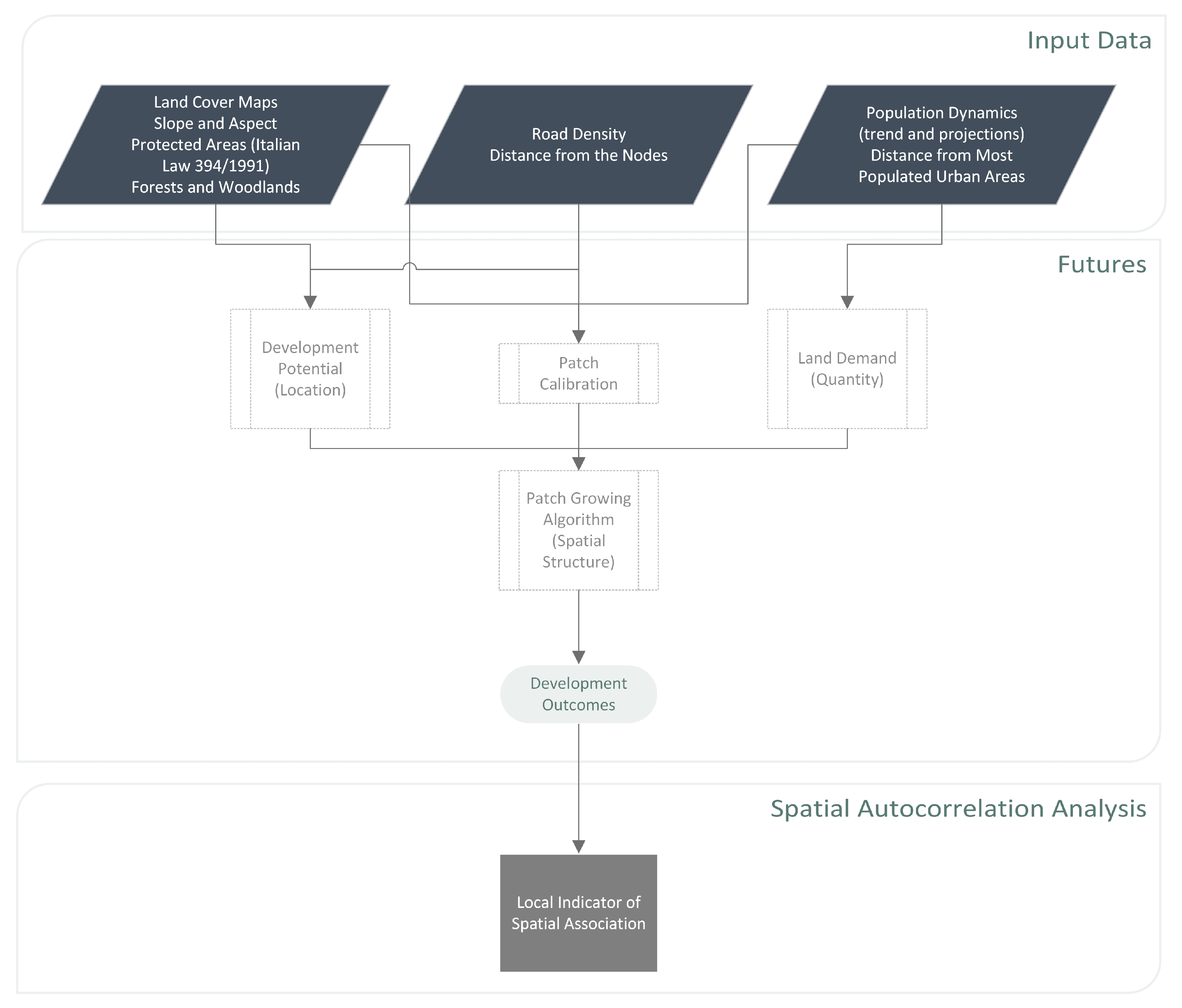
2.1. Model structure
- POTENTIAL, which represents the transition potential model, defining the suitability of each cell to be affected by a transition between land cover classes;
- DEMAND, which represents the change demand model, defining the number of changes expected within each land cover class;
- PGA, or Patch-Growing Algorithm, which represents the change allocation model, defining the location of the expected changes by combining, through a stochastic algorithm, the results of the POTENTIAL and of the DEMAND submodels.
The POTENTIAL submodel uses a multilevel logistic regression technique to generate a map describing the likely positions of future development. This map is used to predict the conversion of a cell from undeveloped to developed. The multilevel logistic regression considers a set of predictive variables which are considered to be relevant for the land cover change dynamics in the study area. These predictive variables can be divided into environmental, infrastructural, and socioeconomic drivers.
The submodel was calibrated based on values detected from a consistent number of randomly sampled points over the study area. Firstly, a seed for the initiation of a patch was allocated randomly across the POTENTIAL probability gradient. The seed survives only if the probability value in POTENTIAL is larger than a random number chosen in the range 0–1. Subsequently, a binary variable was considered, and the probability of the generic cell i changing its state from undeveloped to developed was measured as [45]:
where is the composite suitability score, expressed as:
Specifically, in the equation, ’ is a function of the original development potential, d is the distance of the cell from the seed, and a represents the patch compactness. Hence, when a increases, the cells nearest to the seed become more attractive.
However, the original development potential also depends on the set of environmental, infrastructural, and socioeconomic predictive variables chosen by the user as input for the model. The contribution of these driving forces is measured through the relationship:
where, within the group, h is a predictive variable, is the intercept, n is the number of predictive variables, is the value of h connected to i, is the dynamic development pressure variable, and B is the regression coefficient.
The dynamic development pressure variable is measured as:
in which is a binary variable representing whether the considered cell is developed or not, is the distance between the neighbor cell and the current cell, and g is a coefficient controlling for the influence of the distance and is included in the range 1–100.
Through the multiple regression technique, the POTENTIAL submodel returns for each cell a value included in the range 0–100. These are probability values; higher values indicate that the cell is more likely to change its status from undeveloped to developed. The user can test different combinations and numbers of predictive variables to be included in the regression. An Akaike Information Criterion (AIC) is computed for each combination [46]. This index is used to compare two models, supporting the selection of the one that ensures a better trade-off between model fit and complexity, thus achieving the best predictive ability.
The DEMAND submodel estimates the amount of future development expected in each region of the study area based on population dynamics and urban growth trends. Using the least squares regression technique, the relationship between urban growth and the population variation in each region is considered in terms of the number of inhabitants, generating linear or logarithmic relationships. Specifically, this approach leads to two outputs:
- The relationship between population growth and new development,
- The number of cells that will change their status from undeveloped to developed over the years. Hence, this is the upper limit in the growth of patches during the simulation and, together with the transition potential which is defined as the output of the POTENTIAL submodel, serves as an input file for the PGA submodel.
The PGA submodel simulates the future land cover changes on the basis of an iterative and stochastic selection process, applying a region growing mechanism to change the status of the cells from undeveloped to developed. Hence, this submodel allocates the quantities of changes defined in the DEMAND submodel depending on the suitability of each cell measured through the POTENTIAL submodel. Specifically, only the cells with a suitability value higher than a predefined threshold are considered for the urbanization process. The transition from undeveloped to developed is first experienced by the seeds. Subsequently, the newly urbanized seeds can become the center of new urban patches. This growth continues until the patch reaches a dimension equal to the maximum value defined by the user on the basis of the historical trends of land use changes in the area.
2.2. Study Area and Data Preparation
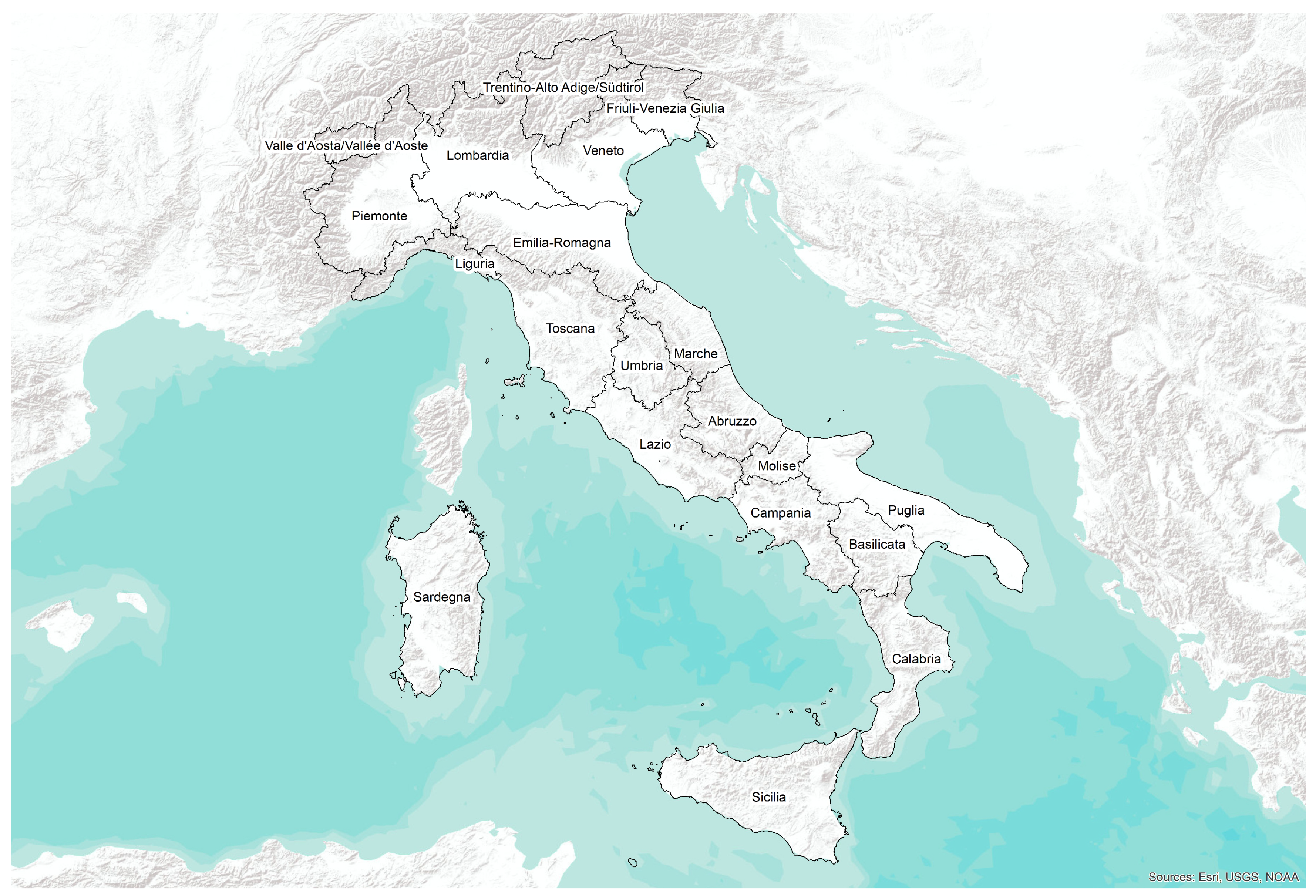
In this study, FUTURES was applied to the case study of urbanization in the Italian national territory (Figure 1).
This is a challenging application, especially because of the wide dimension of the study area and of the country-wide spatial variability in the main drivers that affect urban growth. The analyst, together with the starting conditions of the model, establishes the input data. This is considered the layer to which the growth rules are applied. All data must have the same spatial extension and the same resolution. In this application, a resolution of 100 m was chosen for all the input raster data. The rasters were projected onto the ETRS89 LAEA reference system (EPSG: 3035).
The main input for the model was a collection of time-series maps representing the evolution of urban settlements. Urban areas were extracted from the CORINE land cover maps for the years 1990, 2000, and 2012 [47,48]. These urban extent maps were used in all the three submodels.
For the DEMAND submodel, the historical trends of the population dynamics and their projection to future scenarios are required. For the application in this research, population data were extracted from the Italian National Census database (ISTAT). Specifically, historical data refer to the 2011 census, while the projections were provided by [49].
Finally, to run the DEVELOPMENT submodel, a set of predictive variables must be defined as inputs. In this work, the following rasters were used as predictive variables:
- Slope and aspect. These maps were derived from the DTM available through the Copernicus website [50];
- Distance from water bodies. The water bodies were extracted from the CORINE land cover maps, while the distances were calculated through the GRASSGIS algorithm r.grow.distance;
- Distance from protected areas. The protected areas considered in this application are the assets protected by the Italian National Law 394/1991 on protected areas [51], together with the areas belonging to the Natura 2000 Network regulated by the European directive 92/43/CEE [52]. Data are freely available at [53]. The distance from these areas was measured with the same algorithm used for the distance from water bodies;
- Forests and woodlands. These were extracted from the CORINE land cover maps;
- Travel time from/to the main cities. This predictive variable measures the travel time from/to the cities with higher populations in the country. Travel time is considered as a cumulative cost depending on the distance between two nodes (i.e., two cities) and the maximum speed allowed on the arch (i.e., the road) connecting them. The road network, consisting of highways, national roads, and provincial roads, is available on the Italian National Geoportal [53];
- Road density and distance from the nodes. While the other predictive variables represent a restriction of urbanization, these two predictors favor urban expansion;
- Urban development pressure. This predictor is based on the number of urbanized neighbors of a seed. Higher values of the pressure correspond to a higher probability of a cell being urbanized in the next cycle.
2.3. Spatial Autocorrelation Techniques
In order to verify the simulated data, spatial autocorrelation techniques were adopted based on a measure of the level of similarity between neighboring features to substantiate the geographical reliability of the results. The concept of spatial autocorrelation is based on Waldo Tobler’s first law of geography, “All things are related but nearby things are more related than distant things” [54]. Although this definition is very simple and intuitive [55] and it is a cornerstone of several disciplines, it has not been applied for more than two decades [56]. Only recently has this law been considered again, owing to the spread of spatial models and geographical information systems. The main aim of spatial autocorrelation techniques is to investigate the effects of surrounding objects on a spatial element. There are two main components defining the main geographical object features: location and attributes. In most cases, these components are analyzed separately. Spatial autocorrelation techniques simultaneously analyze the properties and the location of spatial objects [57]. Considering N objects, spatial autocorrelation () can be formalized by the following equation [58]:
where:
- i and j are two objects,
- is the degree of similarity of attributes i and j,
- is the degree of similarity of location i and j.
From this equation, it is possible to determine two global indicators of spatial autocorrelation: the Geary C Ratio [59] and the Moran Index I [60]. The first one computes as the direct difference between the attributes , while the second considers as the difference between the single attributes and and the mean:
These indicators are weak because they only provide information on whether autocorrelation occurs. In order to determine where the highest values of autocorrelation are clustered, it is necessary to adopt local indicators of spatial autocorrelation. There are several indexes for performing such an analysis; in this research, the Local Indicator of Spatial Association () [61] was adopted according to the following formulation:
LISA is often defined as the local Moran and provides a measure of local autocorrelation for each geographic object . The Moran index is proportional to the sum of LISA indexes for each observation:
The spatial properties of global and local indicators of spatial autocorrelation were analyzed using a weight matrix [62], defined as the formal expression of dependence between observations [63]. This matrix is based on the contiguity concept and, according to O’ Sullivan and Unwin [64], it is possible to consider the chess metaphor with respect to the rook, bishop, and queen movements.
3. Results and Discussion
3.1. Potential
Within the POTENTIAL submodel, a set of 12,000 sampling locations have been used to analyse predictors and estimate proper coefficients for the multilevel logistic regression. The boundaries of Italian regions have been included as group level indicator to consider the different behaviours among the different jurisdictional areas of the country. By using a backwards elimination stepwise analysis [65,66], only significant and uncorrelated predictors have been included in the final model, i.e., the one resulting in a lower AIC. A Monte Carlo approach has been used to verify the robustness of this procedure, repeating both the sampling and the model selection 100 times. The fixed effects calculated for the best model are reported in Table 1.
3.2. Demand
The DEMAND submodel returns the output as a graph representing the relationship between population and urban growth. This relationship was measured for each of the 20 Italian regions through linear regression based on the number of developed cells in the raster maps for the years 1990, 2000, and 2012; the population for the same years; and a projection of the population in each region (Figure 2) up to the year 2035. Hence, the linear regression estimates the number of new developed cells expected in the future scenario. In those regions where the Census projections indicate a reduction in the resident population, the number of expected new developed cells was set to zero. Therefore, in those regions, the model did not generate any simulations, which highlights that this model is specifically useful for estimating the share of urban growth due to the real demand, even if this means not considering a number of other phenomena, such as real estate market dynamics.
Sicily, Sardinia, Puglia, Calabria, Basilicata, Molise, and Liguria are therefore totally or almost totally excluded from the simulation. Specifically, the last four regions are expected to have no urban growth at all. This means that, as estimated by this model, there will be no new land development in most of the southern areas of Italy. This is because these regions are characterized by an inversely proportional relationship between the number of inhabitants and the number of developed cells due to a decrease in the resident population. However, an analysis of past trend data highlights the strong push toward the extension of the urbanized areas that has occurred in Southern Italy, particularly in Basilicata (), Molise (), and Apulia (), during the period 2001–2011 [67]. Moreover, a recent analysis by the Italian Institute for the Protection and Environmental Research (ISPRA) showed further increases in the urbanized areas in these regions of , , and , respectively, in the 2016–2017 period alone [68].
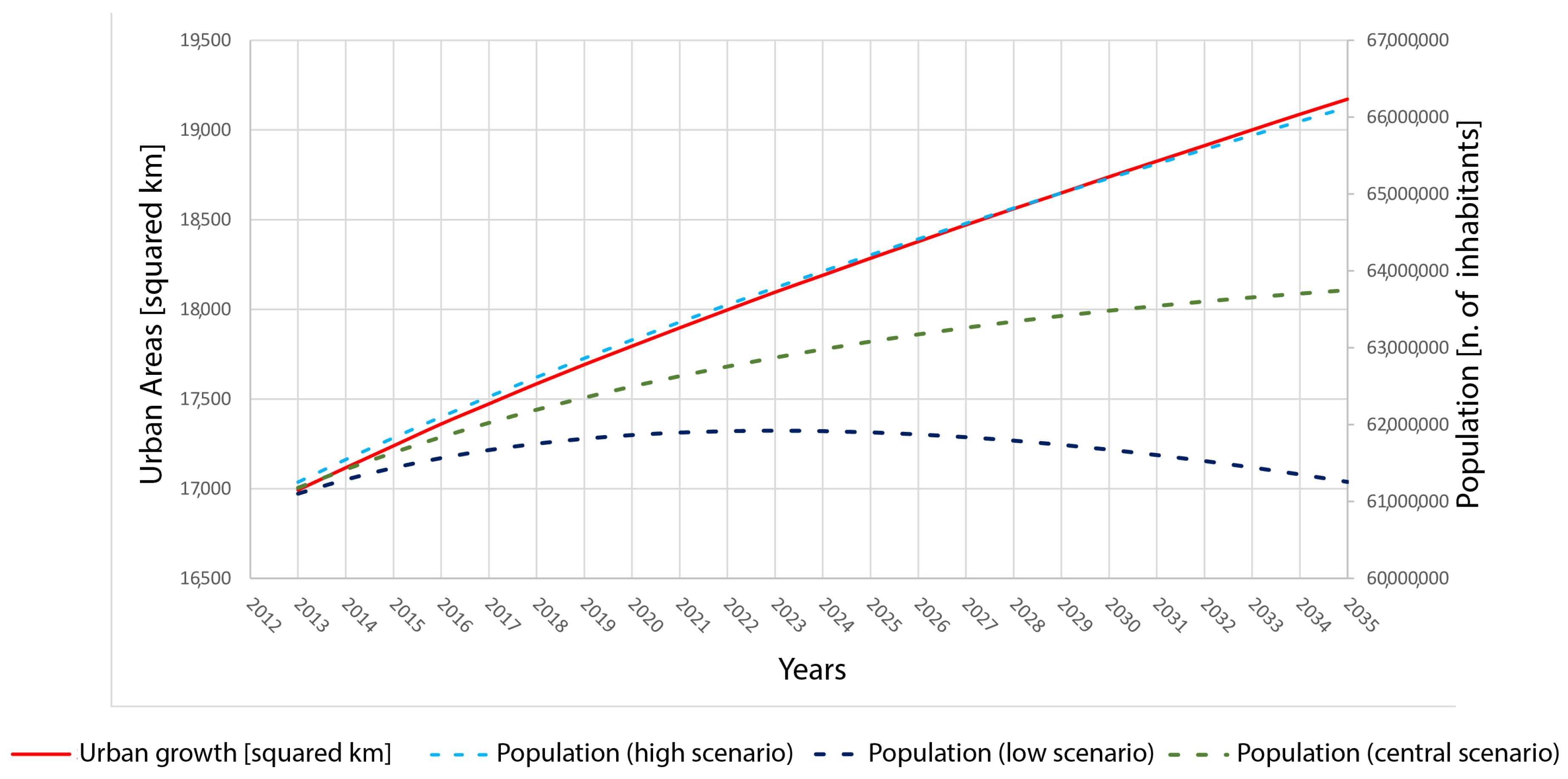
Figure 3 shows the projection of both the urbanized cells and the resident population for the period 2012–2035. The latter was measured for three scenarios based on low, medium, and high rates of population growth. Only the high scenario was tested to calibrate the model to emphasize the relationships between urban growth and population dynamics as considered by the FUTURES model. According to this high scenario, the global population in Italy will reach million by 2051, which implies an increase of 8.2 million since 2007. Figure 3 also shows the high correlation between urban and population growth as indicated by the application of FUTURES. Despite being an expected output, as both urban and population growth are specified to be correlated in the input space of the model, this evidence shows once again how FUTURES overestimates the importance of population dynamics in the simulation process, while there are plenty of other socioeconomic variables that the model does not consider or whose contribution is underestimated. As an example, between 2001 and 2009, new building permits in Italy increased by , while the population only grew by about .
3.3. Patch-Growing Algorithm
The main output of the model is a map representing urbanized areas for future scenarios; this map is produced through the Patch-Growing Algorithm, which stochastically combines the output of the DEMAND and POTENTIAL submodels. In this application, the two parameters discounted factor and compactness (mean) have been selected through the procedure described in [30], resulting in values of 0.3 and 0.2, respectively. It is important to highlight that the stochastic behaviour of PGA is taken into account by reporting the mean value measured over several independent model runs.
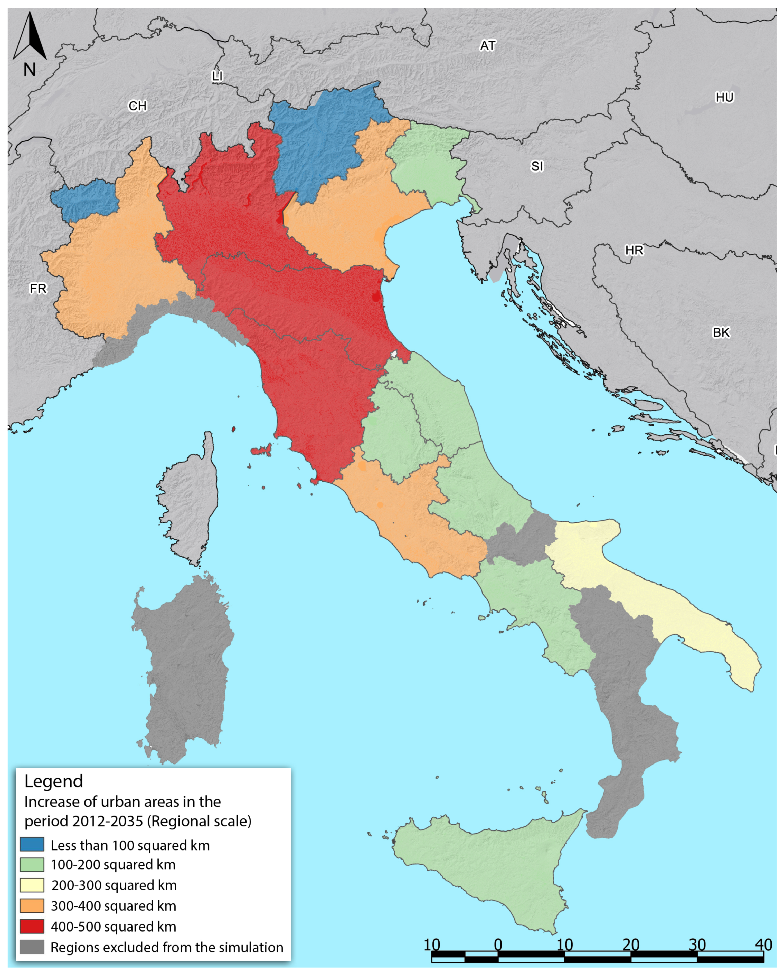
A map of urban areas for the year 2035 was produced. For the period 2012–2035, FUTURES envisages an overall development of urban areas of 3316 km. Five Regions exceed 300 km of new urban areas. The region with the highest quantity of land take is Tuscany with 469.190 km, corresponding to of the entire urban area. Tuscany is followed by Lombardy, with an estimated development of 423.910 km, Emilia Romagna with 414.990 km, Veneto with 374.000 km, and, finally, Piedmont with 304.720 km of new urban areas (Figure 4). A significant development is also expected in Lazio, whose development covers of the total projected development. In Southern Italy, Apulia stands out with 247.470 km, corresponding to of total expected development.
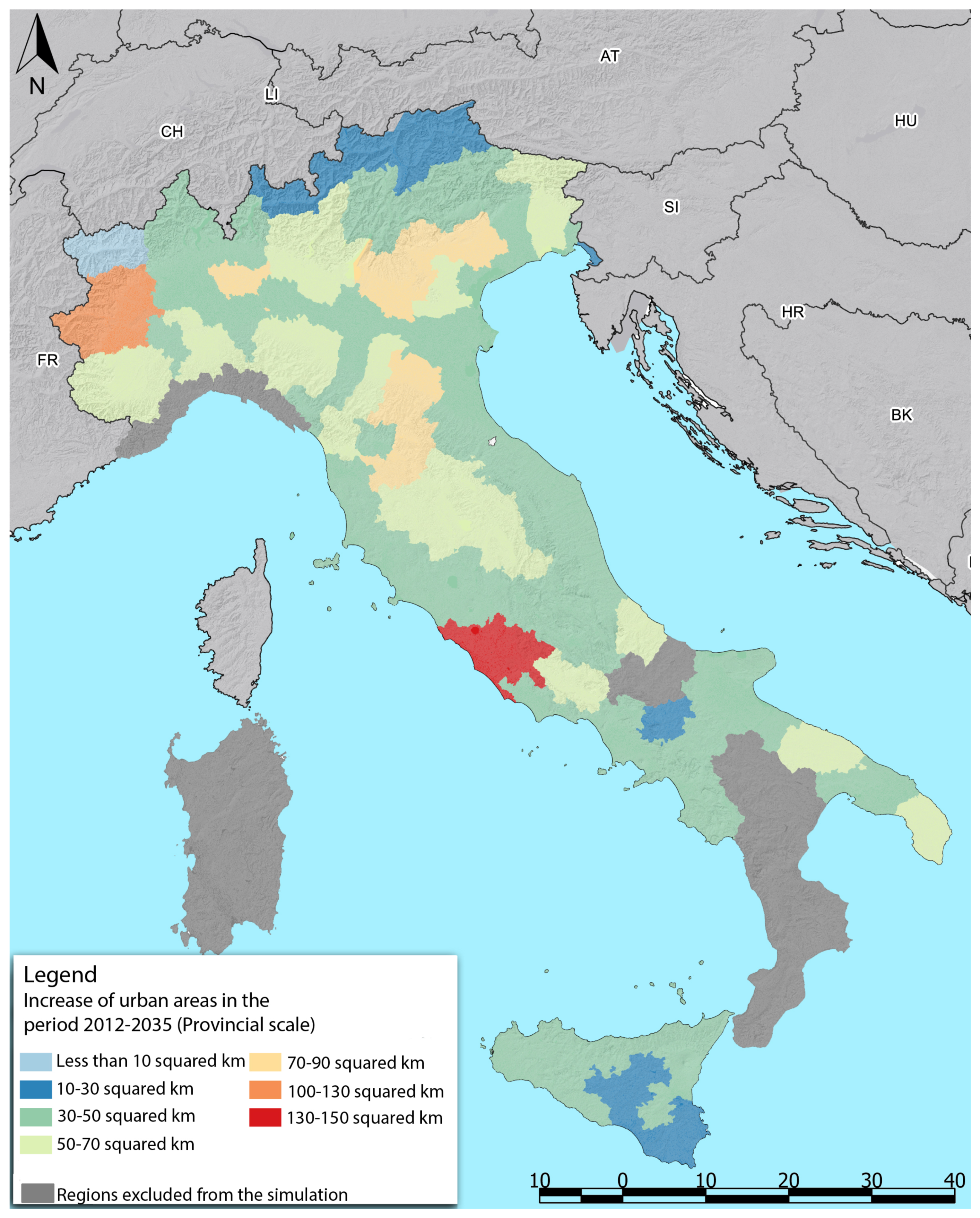
The analysis of the results at the Provincial/Metropolitan scale is also interesting (Figure 5). With 146.700 km, the Metropolitan Area of Rome is the one in which the highest urbanization is expected, covering of the total development expected for the period 2012–2035. The Metropolitan Area of Rome is followed by the Metropolitan Area of Turin with 106.56 km, i.e., of the projected total development. The development is estimated to be between 80 km and 73 km in the Metropolitan Area of Florence; the Provinces of Verona, Bologna, and Vicenza; and the Metropolitan Area of Milan. This is followed by the Provinces Treviso, Udine, Perugia, Lucca, Lecce, Brescia, and Bari, ranging from 70 km to 60 km. Many provinces of Southern Italy, such as Potenza and Matera, are completely excluded from the simulation due to their declining populations.
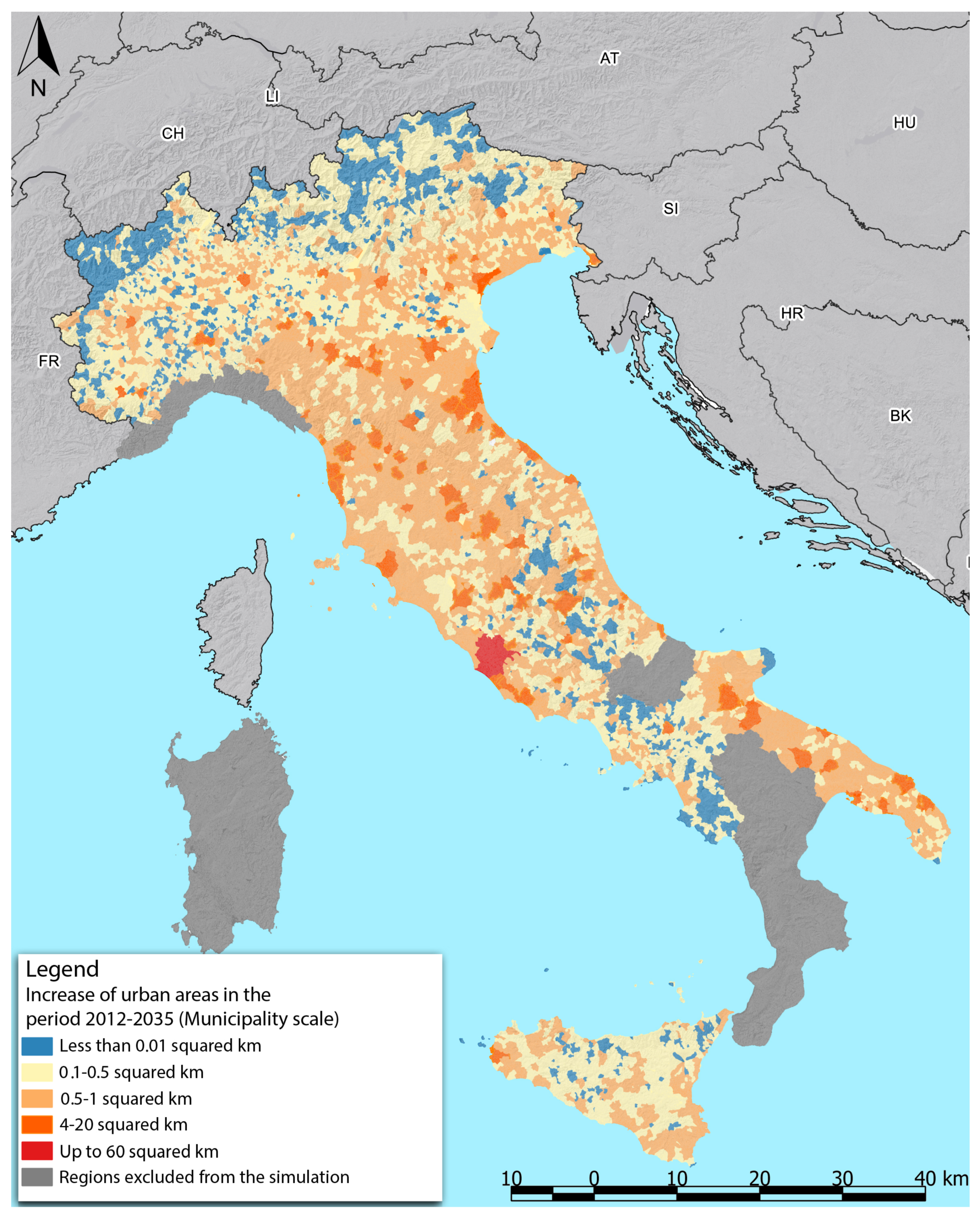
Considering the single municipalities, Rome is estimated to have the largest area of new urbanization at 59.170 km, which covers as much as of the municipal area (Figure 6). Another very widespread municipality is Ravenna, currently 653.259 km, which will grow by about 12.920 km, occupying an extra of the municipal territory. It is also worth noting that some minor municipalities, such as Castelmarte in the Province of Como, which extends for only 1.974 km and is expected to develop 0.780 km, corresponding to of the municipal territory. A similar situation is found for the municipality of Casandrino in the Province of Naples, which is expected to develop of the total municipal area (Figure 7).
The application of FUTURES is of great interest in the urban and spatial planning field, as it integrates demographic features into the scenario-building process for territorial physical aspects. This approach is fundamental in Italy; on the one hand, Italy is very close to the origin of migration and, on the other hand, it has an interest in the important phenomenon of emigration to foreign countries. Today, these analyses are of great significance because they take into account the rapid evolution of demographic dynamics. While in the past, Italy has been considered a destination in migratory phenomena, today there are also other types of dynamics [69,70]. According to the 2018 annual report of the Italian Institute of Statistics [71], “the situation of the country”, immigration from abroad decreased from 527,000 in 2007 to 337,000 in 2017, while emigration abroad has tripled, going from 51,000 to 153,000, with estimated values of 250,000 for 2018. The same report also highlights internal migratory flows. In the period between 2012 and 2016, the internal migration from Southern Italy to the central-northern regions decreased from 132,000 to 108,000; on the contrary, the intensity of migratory flows from southern regions to foreign destinations has almost doubled, from 25,000 to 42,000. Several models do not take into account this kind of data, while, in this case, the results contain demographic aspects. For instance, several regions located in the south are excluded from the simulation because of the reduction in population. This means that urban growth is highly unlikely. Indeed, the increase in urban areas is mainly concentrated along the coastline, in metropolitan areas, and in the most competitive places in the country. These analyses are very useful for supporting decision processes arising from all kinds of plans at the regional and municipality levels. They are also important for analyzing rent and urban land values in the real estate field [72]. Another important aspect to consider is how this approach can support planning activities. The Italian experience is particularly suitable for analyzing the relationship between this simulation and planning documents because master plans are still oversized in terms of new development zones. More specifically, many plans have demographic projections calculated based on the period of the greatest population growth, occurring during the most massive migration from rural to urban areas [73]. The result is a huge availability of development areas in which development has not been implemented at all for more than 20 years. On one hand, this situation forces landowners to pay higher taxes for development rights that probably will never be used. On the other hand, in the most developed areas of the country, these lands are owned by big companies which use these goods to inflate their accounting budget, assigning real estate values higher than reality dictates. The application of this model can be useful in order to support decisions by policymakers to reduce the development zones. This activity is not at all simple because, in the past, the ownership of transformable land has allowed rapid and substantial gains. The adoption of this model can support this process, highlighting in a more objective way where it is better to reduce the development zones and where it is better to keep these areas. These plans also provide an overabundance of infrastructures in all directions. The potential to identify areas of possible expansion can allow for the better management of territory, optimizing services.
3.4. Local Indicator of Spatial Association
To further understand the significance of the output of the model from a geographical point of view, a spatial autocorrelation was measured at the municipality level using the LISA. This index represents a disaggregated measure of the spatial autocorrelation, and it is used to describe the similarity or the dissimilarity of an areal element in comparison with its neighbors.
The use of local spatial autocorrelation indicators does not highlight the concentration of a phenomenon, but the extent of homogeneity of a spatial element compared to the contiguous geographic elements. These indicators are effective in capturing detailed variations in the analyzed variables.
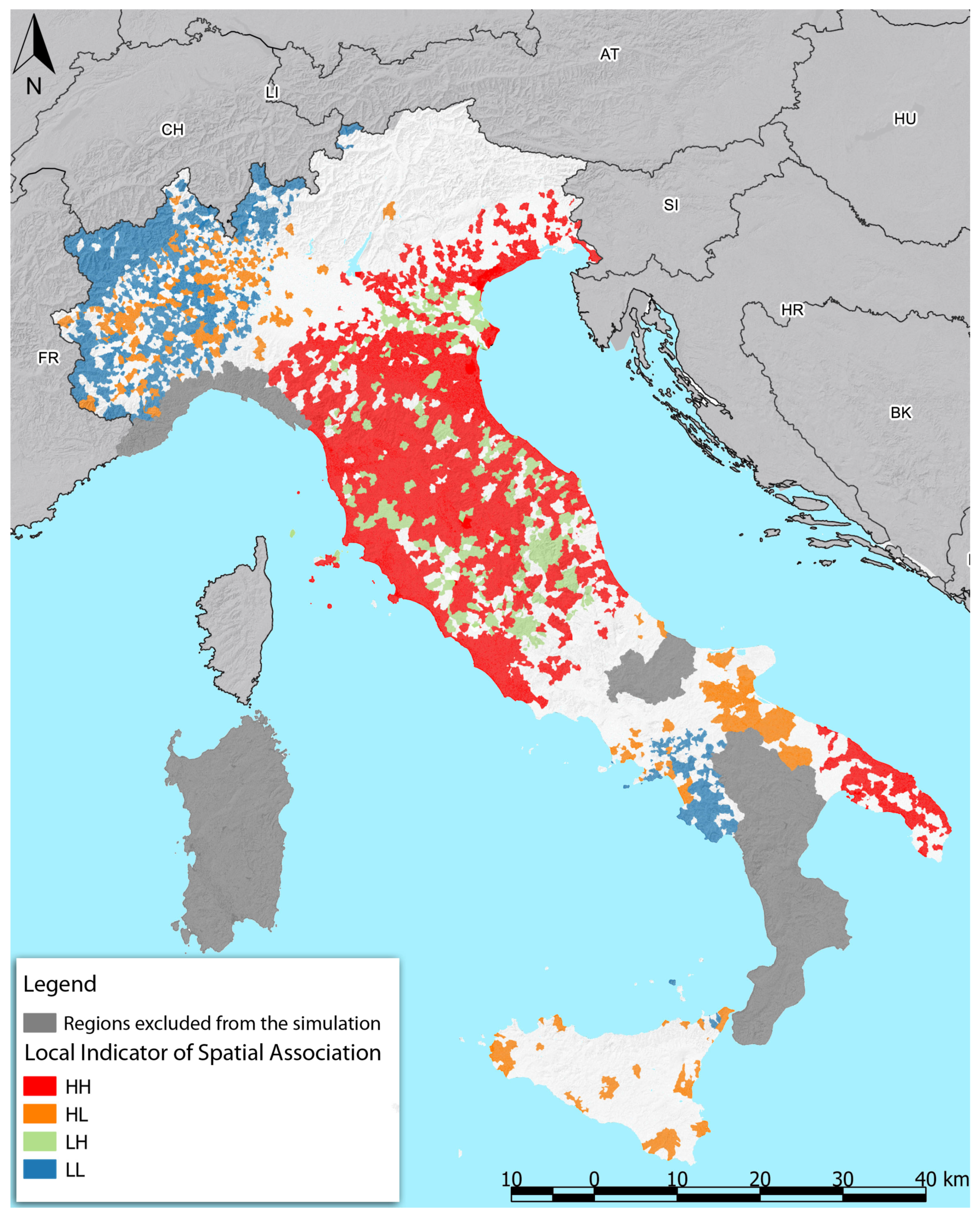
Positive values of the LISA index indicate that both the considered element (in this case, corresponding to a municipality) and its neighbors have high values (H-H) or low values (L-L) of the attribute for which the LISA was measured. On the other hand, negative values indicate behaviors of the areal feature that are different from those of its neighbors: the former has a high value of the attribute while the latter has a low value (H-L combination), or the reverse (L-H). In this case, as the attribute, we used the variation in urbanized soil for each municipality in the period 2012–2035, measured in km. Hence, neighboring municipalities showing similar tendencies toward urbanization will have positive values of the LISA and will become part of a cluster. Figure 8 shows the result of this analysis, using a p-value of and a z-score or (a mapping of the p-values is provided in Supplementary material).
Central Italy shows a high number of clusters having high rates of urbanization (the H-H combination). On the contrary, the Northern part of the country is mainly unclustered, while the Milan area is represented by an H-L combination, showing a tendency of having a huge concentration of its development at the edge of the already existing metropolitan area of the city.
3.5. Model Uncertainty and Soft Classification
Uncertainty plays a primary role in determining the reliability of a model when used as decision support tool. Several authors discussed the role of uncertainty in land suitability analysis, landscape planning [74], environmental assessment [75,76,77], ecosystem services [78] and environmental changes [79]. Two main issues can be identified when dealing with spatial modelling.
Firstly, the combination of the recent technological advances and of the interdisciplinary approach typical of urban and spatial planning can lead to an improper use of data. In numerous cases, geographical analyses are developed using heterogeneous and multi-scale spatial information, generating high uncertainty in the results. This causes a low reliability of the produced informations and a weak support in decision-making [80]. For instance, combining data with different accuracy can produce an error propagation and results can be meaningless or potentially dangerous [81].
Secondly, uncertainty is intrinsically present in every modelling activity [82]. According to Molenaar [83], data model processing stage is based on an interaction between models and processes.
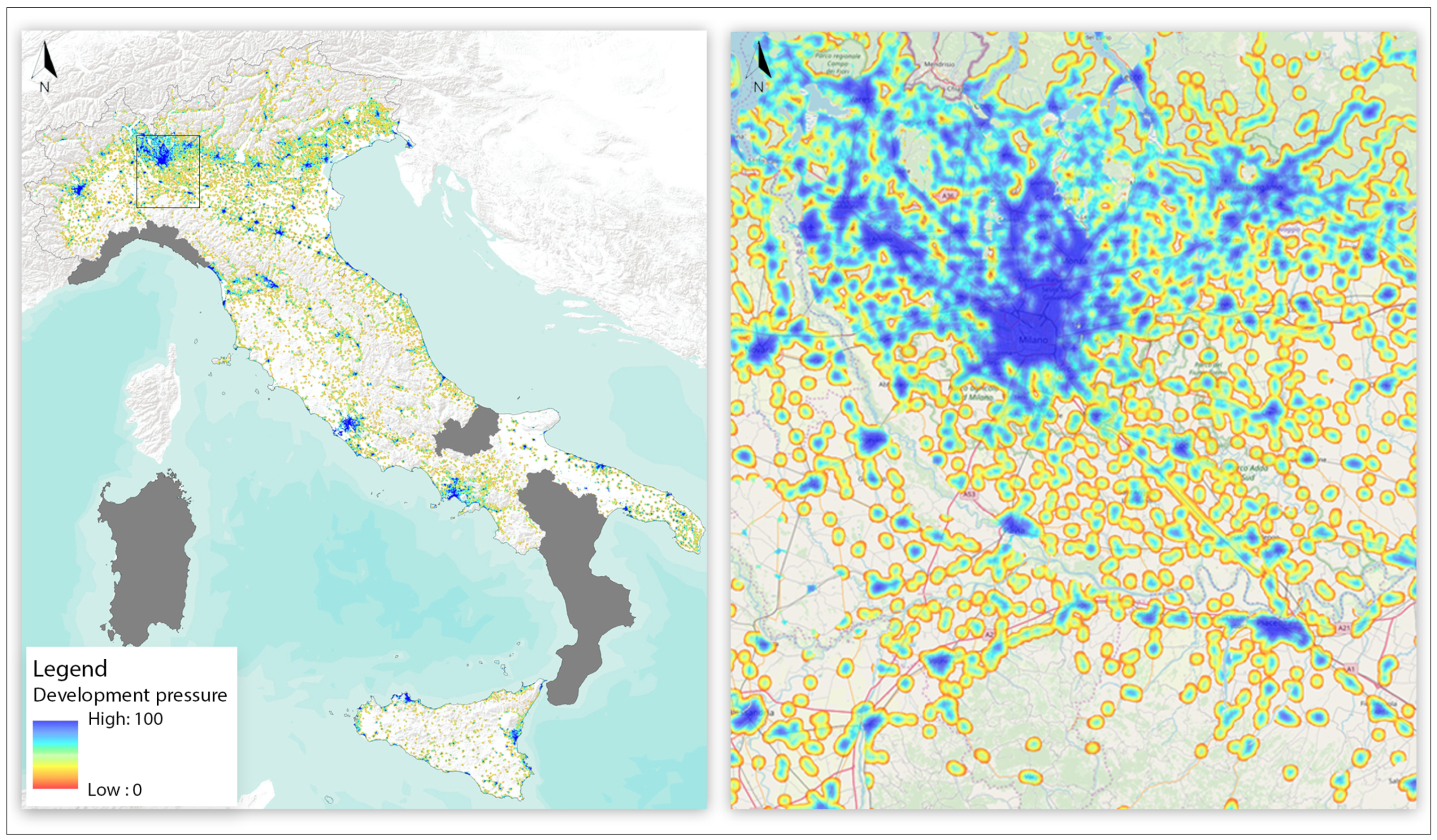
Considering the previously-discussed issues, it is clear the role that uncertainty analysis plays in evaluating the simulation carried out in this paper. The uncertainty in the proposed model is related to two aspects. On the one hand, the driving variables used to calibrate the model have been taken from different sources. On the other, the urban maps resulting from the PGA model are the output of a stochastic hard classification model. For these reasons, it can be extremely useful to consider the output in terms of probability of urbanisation. This soft classification allows keeping into account the uncertainty related to the prediction. The use of this approach to measure uncertainty in Land Use-Land Cover Change Models is a very common approach in literature [84]. Figure 9 shows the soft classification in terms of development pressure resulting from the application of FUTURES.
Leung and Andersson [85] has described the relationship between uncertainty and classical planning theory through four classes, going from a typical Rational Comprehensive kind of plan to a Strategic one.
The first class is an ideal case where it is possible to build a plan with certain objectives based on certain analyses. The result is a set of discrete representations of the physical space which correspond to a set of different values, referring to areas considered homogeneous according to each disciplinary point of view.
The second class is the case of a plan with crisp boundaries, based on fuzzy analyses. If data are imprecise, human evaluation and experience are employed. A typical example is the need to give an answer to a specific problem with certain economic resources.
The third class is very frequent in sector plans (e.g., transport) where the need to achieve widely flexible results and the possibility to obtain several alternatives correspond to a certainty of data.
The fourth class is the case of the strategic plan that identifies the fundamental issues and purposes driving the update process. This is a typical cyclic process where all original choices can be modified and the policy is continually made and re-made, avoiding errors related to radical changes in policy.
Through the soft classification, a richer information is provided to decision-makers, as this map can be interpreted in terms of susceptibility of a territory to urbanisation. This susceptibility map can be extremely useful in the development of the Strategic planning as proposed by Leung and Andersson [85].
4. Conclusions
This paper presents the FUTURES model as a powerful cellular automata tool for estimating urban growth for future scenarios. The main added value of this model when compared to other possible solutions, which are widely discussed in the literature, is the allowance for deep integration with a popular GIS tool, such as GRASSGIS. To ensure the proper execution of the model, homogeneous data must be retrieved for the entire study area to avoid issues during the calibration procedure.
FUTURES could be used as a support tool for the definition of urban plans, as it defines quantities of transformations consistent with the real demand dictated by the dynamics of the population and the spatial dimension of the transformations. It also shows a good capacity for reading the prediction patterns of changes defined according to the system of constraints, attractors, and the presence of mobility infrastructures. These factors can be chosen by the user in the most appropriate way; this represents an advantage, as different simulations can be carried out to investigate the consequences of different scenarios based on a plethora of decision alternatives. As an example, planners could decide whether or not to include protected areas in the constraint framework in order to compare the two results of the simulations and understand the impacts of natural asset protection on urban growth.
The model is based on the real demand dictated by the dynamics of the population. In its application to the Italian urbanization case study, this implies the exclusion of many regions from the simulation. The trend in the population affects the development dynamics. However, it cannot be considered the only driving force influencing urban growth, as there are many other factors that affect development. In FUTURES, demographic trends represent a fundamental index for the estimate of land take. The latter is a multidimensional concept that is influenced by the expansion of urban areas and the loss of biodiversity on natural lands caused by land shifts from natural/woodland cover to agricultural use and by the sealing of natural surfaces. Over the last several decades, these phenomena have increased much more rapidly than the population in Italy, as well as in other European countries. Hence, to estimate the land take and to simulate urban growth, it is not sufficient to consider only the demographic trend as a driving variable. On the contrary, a synthetic index derived from an analysis of all the social and economic factors affecting urban dynamics and settlement dispersion should be used as the main predictive variables. Further studies should, therefore, outline ways to define that index and use it in the simulations carried out using the FUTURES framework.
Supplementary Materials
The following are available online at https://0-www-mdpi-com.brum.beds.ac.uk/2071-1050/10/12/4838/s1, Figure S1: p-values for the measured Local Indicator of Spatial Associations. Only significant values are represented.
Author Contributions
All the authors equally contributed to this research. Specifically, F.A. conceived and designed the experiments; C.C. performed the experiments and analyzed the data; B.M. and F.A. wrote the paper.
Funding
This research received no external funding.
Conflicts of Interest
The authors declare no conflict of interest.
References
- Kareiva, P.M.; Tallis, H.; Ricketts, T.H.; Daily, G.C.; Polasky, S. Natural Capital: Theory and Practice of Mapping Ecosystem Services; Oxford University Press: Oxford, UK, 2011; p. 365. [Google Scholar] [CrossRef]
- Amato, F.; Maimone, B.A.; Martellozzo, F.; Nolè, G.; Murgante, B. The Effects of Urban Policies on the Development of Urban Areas. Sustainability 2016, 8, 297. [Google Scholar] [CrossRef]
- Mcdonald, R.I.; Kareiva, P.; Forman, R.T. The implications of current and future urbanization for global protected areas and biodiversity conservation. Biol. Conserv. 2008, 141, 1695–1703. [Google Scholar] [CrossRef]
- Amato, F.; Pontrandolfi, P.; Murgante, B. Supporting planning activities with the assessment and the prediction of urban sprawl using spatio-temporal analysis. Ecol. Inform. 2015, 30, 365–378. [Google Scholar] [CrossRef]
- Las Casas, G.; Scorza, F. Sustainable Planning: A Methodological Toolkit. In Lecture Notes in Computer Science; Gervasi, O., Murgante, B., Misra, S., Rocha, A.M.A.C., Torre, C., Taniar, D., Apduhan, B.O., Stankova, E., Wang, S., Eds.; Springer International Publishing: Cham, Switzerland, 2016; pp. 627–635. [Google Scholar] [CrossRef]
- Ramankutty, N.; Rhemtulla, J. Can intensive farming save nature? Front. Ecol. Environ. 2012, 10, 455. [Google Scholar] [CrossRef]
- Tajani, F.; Morano, P.; Locurcio, M.; Torre, C.M. Data-driven techniques for mass appraisals. Applications to the residential market of the city of Bari (Italy). Int. J. Bus. Intell. Data Min. 2016, 11, 109. [Google Scholar] [CrossRef]
- United Nations Department of Economic and Social Affairs. 2018 Revision of World Urbanization Prospects; Technical Report; UN: New York, NY, USA, 2018. [Google Scholar]
- Murgante, B.; Borruso, G. Smart cities in a smart world. In Future City Architecture for Optimal Living; Springer International Publishing: Cham, Switzerland, 2015; pp. 13–35. [Google Scholar]
- United Nations Department of Economic and Social Affairs. World Population Ageing 2015; Technical Report; UN: New York, NY, USA, 2015. [Google Scholar]
- Erken, A.; Diaz, M.M.; Engelman, R.; Klugman, J.; Luchsinger, G.; Shaw, E.; Friedman, H.; Barros, A.; Costa, J.; Silva, I.; et al. The State of World Population 2017; Technical Report; UNFPA: New York, NY, USA, 2017. [Google Scholar]
- EEA. Agriculture and the Green Economy; Technical Report; EEA: Luxembourg City, Luxembourg, 2012. [Google Scholar]
- Ramankutty, N.; Coomes, O.T. Land-use regime shifts: An analytical framework and agenda for future land-use research. Ecol. Soc. 2016, 21, 1. [Google Scholar] [CrossRef]
- Foley, J.A.; Ramankutty, N.; Brauman, K.A.; Cassidy, E.S.; Gerber, J.S.; Johnston, M.; Mueller, N.D.; O’connell, C.; Ray, D.K.; West, P.C.; et al. Solutions for a cultivated planet. Nature 2011, 478, 337–342. [Google Scholar] [CrossRef] [PubMed] [Green Version]
- Ramankutty, N. Croplands in West Africa: A Geographically Explicit Dataset for Use in Models. Earth Interact. 2004, 8, 1–22. [Google Scholar] [CrossRef]
- Foley, J.A.; Defries, R.; Asner, G.P.; Barford, C.; Bonan, G.; Carpenter, S.R.; Chapin, F.S.; Coe, M.T.; Daily, G.C.; Gibbs, H.K.; et al. Global consequences of land use. Science 2005, 309, 570–574. [Google Scholar] [CrossRef] [PubMed]
- UN-Habitat. International Guidelines on Urban and Territorial Planning; Technical Report; United Nations Human Settlements Programme (UN-Habitat): Nairobi, Kenya, 2015. [Google Scholar]
- Saganeiti, L.; Amato, F.; Potleca, M.; Nolè, G.; Vona, M.; Murgante, B. Change Detection and Classification of Seismic Damage with LiDAR and RADAR Surveys in Supporting Emergency Planning. The Case of Amatrice; Springer: Cham, Switzerland, 2017. [Google Scholar] [CrossRef]
- Morano, P.; Tajani, F. Saving soil and financial feasibility. A model to support public-private partnerships in the regeneration of abandoned areas. Land Use Policy 2018, 73, 40–48. [Google Scholar] [CrossRef]
- Morano, P.; Tajani, F.; Locurcio, M. GIS application and econometric analysis for the verification of the financial feasibility of roof-top wind turbines in the city of Bari (Italy). Renew. Sustain. Energy Rev. 2017, 70, 999–1010. [Google Scholar] [CrossRef]
- Sallustio, L.; De Toni, A.; Strollo, A.; Di Febbraro, M.; Gissi, E.; Casella, L.; Geneletti, D.; Munafò, M.; Vizzarri, M.; Marchetti, M. Assessing habitat quality in relation to the spatial distribution of protected areas in Italy. J. Environ. Manag. 2017, 201, 129–137. [Google Scholar] [CrossRef] [PubMed]
- Romano, B.; Zullo, F. Half a century of urbanization in southern European lowlands: A study on the Po Valley (Northern Italy). Urban Res. Pract. 2015, 9, 109–130. [Google Scholar] [CrossRef]
- Romano, B.; Zullo, F.; Fiorini, L.; Marcucci, A.; Ciabò, S. Land transformation of Italy due to half a century of urbanization. Land Use Policy 2017, 67, 387–400. [Google Scholar] [CrossRef]
- MacDonald, D.; Crabtree, J.; Wiesinger, G.; Dax, T.; Stamou, N.; Fleury, P.; Gutierrez Lazpita, J.; Gibon, A. Agricultural abandonment in mountain areas of Europe: Environmental consequences and policy response. J. Environ. Manag. 2000, 59, 47–69. [Google Scholar] [CrossRef] [Green Version]
- Marchetti, M.; Ottaviano, M.; Pazzagli, R.; Sallustio, L. Consumo di suolo e analisi dei cambiamenti del paesaggio nei Parchi nazionali d’Italia. Territorio 2013, 121–131. [Google Scholar] [CrossRef]
- Di Palma, F.; Amato, F.; Nolè, G.; Martellozzo, F.; Murgante, B. A SMAP Supervised Classification of Landsat Images for Urban Sprawl Evaluation. ISPRS Int. J. Geo-Inf. 2016, 5, 109. [Google Scholar] [CrossRef]
- Saganeiti, L.; Favale, A.; Pilogallo, A.; Scorza, F.; Murgante, B.; Saganeiti, L.; Favale, A.; Pilogallo, A.; Scorza, F.; Murgante, B. Assessing Urban Fragmentation at Regional Scale Using Sprinkling Indexes. Sustainability 2018, 10, 3274. [Google Scholar] [CrossRef]
- Martellozzo, F.; Amato, F.; Murgante, B.; Clarke, K. Modelling the impact of urban growth on agriculture and natural land in Italy to 2030. Appl. Geogr. 2018, 91, 156–167. [Google Scholar] [CrossRef]
- Scorza, F. Towards Self Energy-Management and Sustainable Citizens’ Engagement in Local Energy Efficiency Agenda. Int. J. Agric. Environ. Inf. Syst. 2016, 7, 44–53. [Google Scholar] [CrossRef]
- Meentemeyer, R.K.; Tang, W.; Dorning, M.A.; Vogler, J.B.; Cunniffe, N.J.; Shoemaker, D.A. FUTURES: Multilevel Simulations of Emerging Urban–Rural Landscape Structure Using a Stochastic Patch-Growing Algorithm. Ann. Assoc. Am. Geogr. 2013, 103, 785–807. [Google Scholar] [CrossRef]
- Benenson, I.; Torrens, P.M. GEosimulation: Automata-Based Modeling of Urban Phenomena; John Wiley & Sons, Ltd.: West Sussex, UK, 2004. [Google Scholar] [CrossRef]
- Verburg, P.H.; Schot, P.P.; Dijst, M.J.; Veldkamp, A. Land use change modelling: Current practice and research priorities. GeoJournal 2004, 61, 309–324. [Google Scholar] [CrossRef]
- Kityuttachai, K.; Tripathi, N.; Tipdecho, T.; Shrestha, R. CA-Markov Analysis of Constrained Coastal Urban Growth Modeling: Hua Hin Seaside City, Thailand. Sustainability 2013, 5, 1480–1500. [Google Scholar] [CrossRef] [Green Version]
- Yang, J.; Lee, H. An AHP decision model for facility location selection. Facilities 1997, 15, 241–254. [Google Scholar] [CrossRef]
- Schoier, G.; Borruso, G. A methodology for dealing with spatial big data. Int. J. Business Intell. Data Min. 2017, 12, 1–13. [Google Scholar] [CrossRef]
- Onsted, J.; Clarke, K.C. The inclusion of differentially assessed lands in urban growth model calibration: A comparison of two approaches using SLEUTH. Int. J. Geogr. Inf. Sci. 2012, 26, 881–898. [Google Scholar] [CrossRef]
- Martellozzo, F.; Clarke, K.C. Measuring urban sprawl, coalescence, and dispersal: A case study of Pordenone, Italy. Environ. Plan. B Plan. Des. 2011, 38, 1085–1104. [Google Scholar] [CrossRef]
- Amato, F.; Martellozzo, F.; Nolè, G.; Murgante, B. Preserving cultural heritage by supporting landscape planning with quantitative predictions of soil consumption. J. Cult. Herit. 2017, 23, 44–54. [Google Scholar] [CrossRef]
- Amato, F.; Pontrandolfi, P.; Murgante, B. Using Spatiotemporal Analysis in Urban Sprawl Assessment and Prediction; Springer: Cham, Switzerland, 2014. [Google Scholar] [CrossRef]
- Petrasova, A.; Petras, V.; Shoemaker, D.A.; Dorning, M.A.; Meentemeyer, R.K. The Integration of Land Change Modeling Framework FUTURES into GRASS GIS 7. Available online: https://petrasovaa.github.io/publications/futures_integration_presentation.pdf (accessed on 13 December 2018).
- Clarke, K.C. Cellular Automata and Agent-Based Models. In Handbook of Regional Science; Springer: Berlin/Heidelberg, Germnay, 2014; pp. 1217–1233. [Google Scholar] [CrossRef]
- Pinto, N.; Antunes, A.; Roca, J. Cellular Automata in Urban Simulation: Basic Notions and Recent Developments. In Handbook of Theoretical and Quantitative Geography; Faculty of Geosciences and Environment: Lausanne, Switzerland, 2009. [Google Scholar]
- Batty, M.; Coucelis, H.; Eichen, M. Urban systems as cellular automata. Environ. Plan. B Plan. Des. 1997, 24, 159–164. [Google Scholar] [CrossRef]
- Dorning, M.A.; Koch, J.; Shoemaker, D.A.; Meentemeyer, R.K. Simulating urbanization scenarios reveals tradeoffs between conservation planning strategies. Landsc. Urban Plan. 2015, 136, 28–39. [Google Scholar] [CrossRef]
- Bolker, B.M.; Brooks, M.E.; Clark, C.J.; Geange, S.W.; Poulsen, J.R.; Stevens, M.H.H.; White, J.S.S. Generalized linear mixed models: A practical guide for ecology and evolution. Trends Ecol. Evol. 2009, 24, 127–135. [Google Scholar] [CrossRef] [PubMed]
- Akaike, H. Akaike’s Information Criterion. In International Encyclopedia of Statistical Science; Springer: Berlin/Heidelberg, Germany, 2011; p. 25. [Google Scholar] [CrossRef]
- EEA. CORINE Land Cove—Part 1: Methodology. Technical Report. Available online: https://www.eea.europa.eu/publications/COR0-part1 (accessed on 13 December 2018).
- Copernicus Programme. CORINE Land Cover. Available online: http://land.copernicus.eu/pan-european/corine-land-cover (accessed on 13 December 2018).
- ISTAT. Il Futuro Demgrafico del Paese; Technical Report; ISTAT: Rome, Italy, 2011.
- Copernicus. The Copernicus Open Access Hub. Available online: https://scihub.copernicus.eu/dhus/ (accessed on 13 December 2018).
- Italian Parlament. Decreto Legislativo 22 gennaio 2004, n. 42; Codice dei beni culturali e del paesaggio, ai sensi dell’articolo 10 della legge 6 luglio 2002, n. 137. Available online: http://www.parlamento.it/parlam/leggi/deleghe/04042dl.htm (accessed on 13 December 2018).
- Council Directive 92/43/EEC on the Conservation of Natural Habitats and of Wild Fauna and Flora; Council of the European Union: Bruxelles, Belgium, 21 May 1992.
- Geoportale Nazionale. 2017. Available online: http://www.pcn.minambiente.it/mattm/ (accessed on 13 December 2018).
- Tobler, W.R. A Computer Movie Simulating Urban Growth in the Detroit Region. Econ. Geogr. 1970, 46, 234. [Google Scholar] [CrossRef]
- Tobler, W. On the First Law of Geography: A Reply. Ann. Assoc. Am. Geogr. 2004, 94, 304–310. [Google Scholar] [CrossRef]
- Sui, D.Z. Tobler’s First Law of Geography: A Big Idea for a Small World? Ann. Assoc. Am. Geogr. 2004, 94, 269–277. [Google Scholar] [CrossRef]
- Goodchild, M.F. Spatial Autocorrelation; GeoBooks: Norwich, England, 1986; Volume 47. [Google Scholar]
- Lee, J.; Wong, D. Statistical Analysis with ArcView GIS; John Wiley & Sons: New York, NY, USA, 2001. [Google Scholar]
- Geary, R.C. The Contiguity Ratio and Statistical Mapping. Inc. Stat. 1954, 5, 115. [Google Scholar] [CrossRef]
- Moran, P.A. The interpretation of statistical maps. J. R. Stat. Soc. Ser. B 1948, 10, 243–251. [Google Scholar] [CrossRef]
- Anselin, L. Spatial Econometrics: Methods and Models; Kluwer Academic: Dordrecht, The Netherlands, 1988. [Google Scholar]
- Cliff, A.D.; Ord, K. Spatial Autocorrelation: A Review of Existing and New Measures with Applications. Econ. Geogr. 1970, 46, 269. [Google Scholar] [CrossRef]
- Anselin, L. Local Indicators of Spatial Association-LISA. Geogr. Anal. 2010, 27, 93–115. [Google Scholar] [CrossRef]
- O’sullivan, D.; Unwin, D. Geographic Information Analysis; John Wiley & Sons: Hoboken, NJ, USA, 2014. [Google Scholar]
- Derksen, S.; Keselman, H.J. Backward, forward and stepwise automated subset selection algorithms: Frequency of obtaining authentic and noise variables. Br. J. Math. Stat. Psychol. 1992, 45, 265–282. [Google Scholar] [CrossRef]
- Holland, J.; Goldberg, D. Genetic Algorithms in Search, Optimization and Machine Learning; Addison-Wesley: Boston, MA, USA, 1989. [Google Scholar]
- Basi territoriali e variabili censuarie. Available online: https://www.istat.it/it/archivio/104317 (accessed on 13 December 2018).
- Istituto Superiore per la Protezione e la Ricerca Ambientale. Consumo di Suolo, Dinamiche Territoriali E Servizi Ecosistemici; ISPRA: Roma, Italy, 2018. [Google Scholar]
- Scardaccione, G.; Scorza, F.; Las Casas, G.; Murgante, B. Spatial Autocorrelation Analysis for the Evaluation of Migration Flows: The Italian Case. In Lecture Notes in Computer Science; Taniar, D., Gervasi, O., Murgante, B., Pardede, E., Apduhan, B.O., Eds.; Springer: Berlin/Heidelberg, Germany, 2010; pp. 62–76. [Google Scholar] [CrossRef]
- Murgante, B.; Borruso, G. Analyzing Migration Phenomena with Spatial Autocorrelation Techniques; Springer: Berlin/Heidelberg, Germany, 2012; pp. 670–685. [Google Scholar] [CrossRef]
- Italian Institute of Statistics. La Situazione del Paese; Technical Report; ISTAT: Roma, Italy, 2018.
- Manganelli, B.; Murgante, B.; Manganelli, B.; Murgante, B. The Dynamics of Urban Land Rent in Italian Regional Capital Cities. Land 2017, 6, 54. [Google Scholar] [CrossRef]
- Romano, B.; Zullo, F.; Marucci, A.; Fiorini, L. Vintage Urban Planning in Italy: Land Management with the Tools of the Mid-Twentieth Century. Sustainability 2018, 10, 4125. [Google Scholar] [CrossRef]
- Neuendorf, F.; von Haaren, C.; Albert, C. Assessing and coping with uncertainties in landscape planning: An overview. Landsc. Ecol. 2018, 33, 861–878. [Google Scholar] [CrossRef]
- Bodde, M.; van der Wel, K.; Driessen, P.; Wardekker, A.; Runhaar, H.; Bodde, M.; van der Wel, K.; Driessen, P.; Wardekker, A.; Runhaar, H. Strategies for Dealing with Uncertainties in Strategic Environmental Assessment: An Analytical Framework Illustrated with Case Studies from The Netherlands. Sustainability 2018, 10, 2463. [Google Scholar] [CrossRef]
- Leung, W.; Noble, B.; Gunn, J.; Jaeger, J.A. A review of uncertainty research in impact assessment. Environ. Impact Assess. Rev. 2015, 50, 116–123. [Google Scholar] [CrossRef]
- Dorini, G.; Kapelan, Z.; Azapagic, A. Managing uncertainty in multiple-criteria decision making related to sustainability assessment. Clean Technol. Environ. Policy 2011, 13, 133–139. [Google Scholar] [CrossRef]
- Bryant, B.P.; Borsuk, M.E.; Hamel, P.; Oleson, K.L.; Schulp, C. Transparent and feasible uncertainty assessment adds value to applied ecosystem services modeling. Ecosyst. Serv. 2018, 33, 103–109. [Google Scholar] [CrossRef]
- Polasky, S.; Carpenter, S.R.; Folke, C.; Keeler, B. Decision-making under great uncertainty: Environmental management in an era of global change. Trends Ecol. Evol. 2011, 26, 398–404. [Google Scholar] [CrossRef] [PubMed]
- Walker, W.; Harremoës, P.; Rotmans, J.; van der Sluijs, J.; van Asselt, M.; Janssen, P.; Krayer von Krauss, M. Defining Uncertainty: A Conceptual Basis for Uncertainty Management in Model-Based Decision Support. Integr. Assess. 2003, 4, 5–17. [Google Scholar] [CrossRef] [Green Version]
- Zhang, J.; Goodchild, M.F.; Goodchild, M.F. Uncertainty in Geographical Information; CRC Press: London, UK, 2002. [Google Scholar] [CrossRef]
- Fischhoff, B.; Davis, A.L. Communicating scientific uncertainty. Proc. Natl. Acad. Sci. USA 2014, 111, 13664–13671. [Google Scholar] [CrossRef] [PubMed] [Green Version]
- Molenaar, M. An Introduction to the Theory of Spatial Object Modelling For GIS; Taylor & Francis: London, UK, 1998; p. 246. [Google Scholar]
- Amato, F.; Tonini, M.; Murgante, B.; Kanevski, M. Fuzzy definition of Rural Urban Interface: An application based on land use change scenarios in Portugal. Environ. Modell. Softw. 2018, 104, 171–187. [Google Scholar] [CrossRef]
- Leung, Y.; Andersson, A.E. Spatial Analysis and Planning under Imprecision; Elsevier Science: Amsterdam, The Netherlands, 2013; p. 392. [Google Scholar]
Figure 1.
The flowchart of the application proposed in this paper.

Figure 2.
The study area and the subnational boundaries of the regions.

Figure 3.
Projection of urban growth made through FUTURES compared to the projections of population growth made by the Italian National Census Institute (ISTAT). Only the high-population scenario was considered in the simulation.
Figure 3.
Projection of urban growth made through FUTURES compared to the projections of population growth made by the Italian National Census Institute (ISTAT). Only the high-population scenario was considered in the simulation.

Figure 4.
Variation in the extension of urban areas for the period 2012–2035 at the regional scale.

Figure 5.
Variation in the extension of urban areas in the period 2012–2035 at the Provincial/Metropolitan Area scale.
Figure 5.
Variation in the extension of urban areas in the period 2012–2035 at the Provincial/Metropolitan Area scale.

Figure 6.
Variation in the extension of urban areas in the period 2012–2035 on the municipal scale.

Figure 7.
Urban growth expected through the simulation during the period 2012–2035 in the main Italian municipalities (from top to bottom and from left to right) Rome, Bari, Milan, Naples, Venice Padua and Treviso, Florence, Bologna, and Ravenna.
Figure 7.
Urban growth expected through the simulation during the period 2012–2035 in the main Italian municipalities (from top to bottom and from left to right) Rome, Bari, Milan, Naples, Venice Padua and Treviso, Florence, Bologna, and Ravenna.

Figure 8.
Local Indicators of Spatial Association index measurement of the variation in the extension of urban areas in the period 2012–2035 at the municipal scale.
Figure 8.
Local Indicators of Spatial Association index measurement of the variation in the extension of urban areas in the period 2012–2035 at the municipal scale.

Figure 9.
Soft classification expressed in terms of development pressure for Italy (left) and a zoom on the Milan metropolitan area (right). Low values correspond to a lower susceptibility to urbanisation, while higher values correspond to higher probabilities.
Figure 9.
Soft classification expressed in terms of development pressure for Italy (left) and a zoom on the Milan metropolitan area (right). Low values correspond to a lower susceptibility to urbanisation, while higher values correspond to higher probabilities.


Table 1.
Results of the selected generalized linear mixed model fit by maximum likelihood (Laplace Approximation)—fixed effects.
Table 1.
Results of the selected generalized linear mixed model fit by maximum likelihood (Laplace Approximation)—fixed effects.
| Estimate | Std. Error | p-Value | |
|---|---|---|---|
| Intercept (varies by region) | −4.558 | 0.137 | <0.001 |
| Development pressure | 0.270 | 0.006 | <0.001 |
| Slope | −0.049 | 0.009 | <0.001 |
| Percentage of Forests | 0.005 | 0.002 | 0.050 |
| Distance from nodes | 0.092 | 0.032 | 0.004 |
| Travel time | 0.039 | 0.008 | <0.001 |
© 2018 by the authors. Licensee MDPI, Basel, Switzerland. This article is an open access article distributed under the terms and conditions of the Creative Commons Attribution (CC BY) license (http://creativecommons.org/licenses/by/4.0/).
Share and Cite
MDPI and ACS Style
Cosentino, C.; Amato, F.; Murgante, B. Population-Based Simulation of Urban Growth: The Italian Case Study. Sustainability 2018, 10, 4838. https://0-doi-org.brum.beds.ac.uk/10.3390/su10124838
AMA Style
Cosentino C, Amato F, Murgante B. Population-Based Simulation of Urban Growth: The Italian Case Study. Sustainability. 2018; 10(12):4838. https://0-doi-org.brum.beds.ac.uk/10.3390/su10124838
Chicago/Turabian StyleCosentino, Claudia, Federico Amato, and Beniamino Murgante. 2018. "Population-Based Simulation of Urban Growth: The Italian Case Study" Sustainability 10, no. 12: 4838. https://0-doi-org.brum.beds.ac.uk/10.3390/su10124838
Note that from the first issue of 2016, this journal uses article numbers instead of page numbers. See further details here.