Can More Environmental Information Disclosure Lead to Higher Eco-Efficiency? Evidence from China


School of Economics and Trade, Hunan University, 109 Road Shijiachong, Yuelu District, Changsha 410079, China
*
Author to whom correspondence should be addressed.
Sustainability 2018, 10(2), 528; https://0-doi-org.brum.beds.ac.uk/10.3390/su10020528
Submission received: 6 December 2017
/
Revised: 6 February 2018
/
Accepted: 12 February 2018
/
Published: 15 February 2018
Abstract
:The present paper investigates the impact of pollution information transparency index (PITI) on eco-efficiency using a novel panel dataset covering 109 key environmental protection prefecture-level cities in China over the period 2008–2015. We apply an extended data envelopment analysis (DEA) model, simultaneously incorporating metafrontier, undesirable outputs and super efficiency into slack-based measure (Meta-US-SBM) to estimate eco-efficiency. Then, the bootstrap Granger causality approach is utilized to test the unidirectional Granger causal relationship running from PITI to eco-efficiency. Results of DEA model show that there exist significant spatiotemporal disparities of eco-efficiency, on average, the eco-efficiency in eastern region is relative higher than those of central/western region. Estimates of ordinary least square (OLS) method, quantile regression, and spatial Durbin model document that the evidence of an inverted-U-shaped relation between PITI and eco-efficiency is supported, and the turning points vary from 0.3370 to 0.4540 with different model specifications. Finally, supplementary analysis of panel threshold model also supports the robust findings. Policy implications are presented based on the empirical results.
1. Introduction
In this study, we investigate how environmental information disclosure of Chinese prefecture-level cities relates to eco-efficiency [1]. More specifically, we examine the association between the pollution information transparency index (henceforth PITI, maximum value is 100) and eco-efficiency measured by an extended DEA model [2], simultaneously incorporating the presence of metafrontier technique, undesirable outputs, and super efficiency into slacks-based measure (henceforth Meta-US-SBM). (The World Business Council for Sustainable Development (WBCSD) defines eco-efficiency as the reducing environmental impact and resource intensity in the process of satisfying human needs and bringing quality of life [3]. Up to date, eco-efficiency has been widely utilized to measure sustainability for varied levels in existing literature [4,5,6,7,8,9,10,11]) We focus on the impact PITI exerts on eco-efficiency from both non-spatial and spatial model specifications.
Extensive studies have been devoted to studying environmental disclosure, which will impose either positive effect on sustainability performance [12,13], or negative effect on sustainability performance [14,15]. From the micro-level (e.g., enterprises, companies, and institutions), however, a multitude of studies on analyzing the environmental information disclosure has been conducted in the academic community [16,17,18,19]. If government information were more transparent, it would be more beneficial to the improvement of eco-efficiency [20]. Prior research has not yet established a consistent understanding regarding the relationship between environmental disclosure and eco-efficiency; rare studies have shown whether there exists unidirectional or bidirectional relation between environmental information disclosure and eco-efficiency [21]. On the one hand, following the voluntary disclosure theory [22], a region/city with incentive to disclose information is conducive to reduce pollutant emissions, thus leading to promoting eco-efficiency. On the other hand, a region/city without incentive to disclose information is reluctant to reduce pollutant emissions, consequently resulting in lower eco-efficiency, as predicted by legitimacy theory [23,24]. However, the two theories are not necessarily contradictory but are instead two sides of the same coin [25]. Thus, we suppose that there may exist a tradeoff between PITI and eco-efficiency of prefecture-level cities in China. Specifically, environmental information disclosure has been advocated by the government; managers/policymakers believe that disclosing more environmental information can be fully detected by government, enabling them to access more such resource elements as technology and labor force, leading to improve eco-efficiency overall. With this scenario, the PITI is positively associated with eco-efficiency before the PITI reaches the threshold value. Otherwise, the PITI is negatively associated with eco-efficiency after the threshold value, which resulted from regulators having limited supervision of the vast amount of information with the increase of environmental information disclosure, along with the increase potential costs of litigation risk caused by environmental information disclosure.
The main contributions of this article are as follows. First, we use Meta-US-SBM model to evaluate eco-efficiency of prefecture-level cities in China. The strengths of Meta-US-SBM are its comparable treatment of efficiency of the same DMU in different years due to technological progress to consider the metafrontier [26]; its identifiable treatment of DMUs located on efficient frontier to consider super efficiency [27]; and its similar to the real production process when considering undesirable outputs. Second, we explore the impacts of PITI on eco-efficiency based on non-spatial and spatial econometric methods. Policy implications are provided based on the empirical results.
2. Methodology and Empirical Strategy
2.1. Measuring Environmental Information Disclosure in China
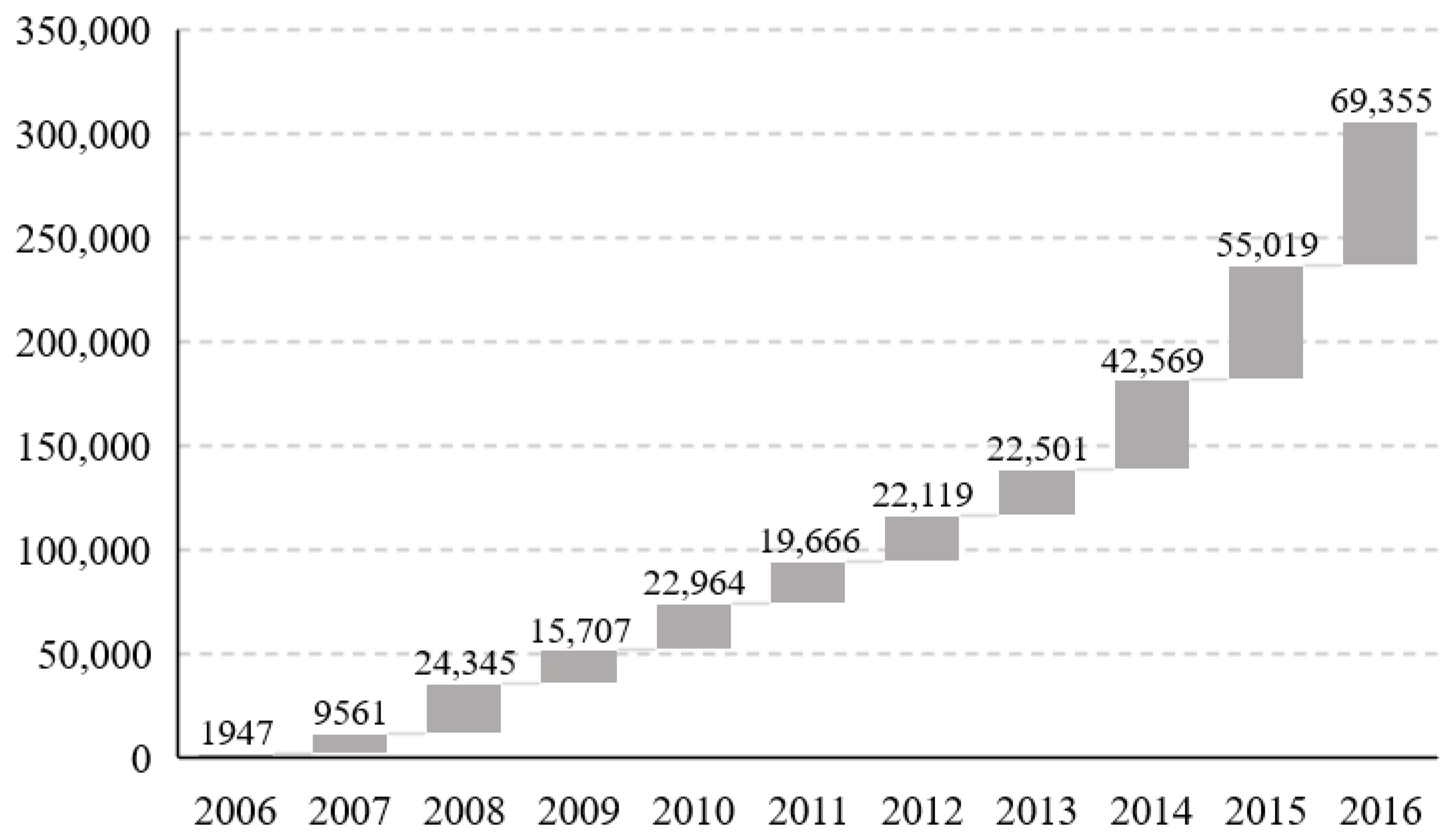
The major breakthroughs in Chinese environmental information disclosure occurred after 2007, but the first formal government initiatives on environmental information disclosure date to 1999–2000. Then, environmental information disclosure gradually expanded. The concepts of disclosure and public participation are included in the 2003 Environmental Impact Assessment (EIA) Law and the 2004 Administrative Licensing Law (ALL). Environmental regulators were the first to promulgate implementing rules pursuant to the State Council Regulation on Open Government Information, a signal of support for disclosure. In recent years, China has adopted several measures for information disclosure; more details can be found in the latest work of [28], which examines the emergence of environmental information disclosure in China. Since 2008, the Institute of Public & Environmental Affairs and Natural Resource Defense Council evaluate PITI for the periods of 2008–2016, providing the details of evaluation method and criteria, and alleviating the difficulties of measuring information disclosure in China. Figure 1 illustrates the total amount of pollution monitoring records during 2006–2016, indicating that the geometrical growth rate of pollution monitoring records is approximately 43%. Theoretically, for a region/city, more environmental information disclosure leads to desire to reduce pollutant emissions, thus improving eco-efficiency. Empirically, however, it is worth studying whether there exists a nonlinear relation between PITI and eco-efficiency; as a result, the impact PITI exerts on eco-efficiency may show a threshold effect or interval effect. In econometric models, the key explanation variable (PITI) is directly collected from Institute of Public & Environmental Affairs (IPE) and Natural Resource Defense Council (NRDC) and converted to the proportion form (maximum value is 1).
2.2. Measuring Eco-Efficiency with Meta-US-SBM Model
If there are DMUs (prefecture-level cities in this study), technology-heterogeneous groups (in China, we considered three regions: eastern, central and western) and DMUs in Group , we have . Each DMU uses inputs to produce desirable (good) outputs and undesirable (bad) outputs . The frontier production technology of Group can be expressed as follows:
where is a weighting vector of nth DMU in Group with reference to the corresponding group frontier. By enveloping all group frontier technologies [26], we can also express the metafrontier production technology as follows:
where and is a weighting vector of the nth DMU in Group with reference to the metafrontier. With group frontier and metafrontier defined, we can now define non-oriented super efficiency SBMs for both frontiers. Assuming constant returns to scale (CRS), the optimal objective value for the oth DMU in Group (; ) with reference to the group frontier is estimated as:
and the same for the oth DMU in Group (; ) with reference to the metafrontier is estimated as:
where in Model (3) and in Model (4) are nonnegative weights, and , , and represent, respectively, the input, desirable output, and undesirable output slacks. The difference between the super efficiency model and the standard model is that DMUko in the reference set in the super efficiency model is excluded [27], which is denoted by . Adding the constraints to Equation (3) and to Equation (4) will impose the variable returns to scale (VRS) assumption. The term is non-Archimedean infinitely small and the corresponding constraint ensuring the denominator in objective function greater than zero.
2.3. Empirical Strategy
Empirical approaches such as ordinary least square (OLS) regression, quantile regression, and spatial econometric model are used throughout this paper. Firstly, for the sake of simplicity, to investigate the nonlinear relationship between PITI and eco-efficiency, we introduce the quadratic term of PITI into the baseline model, which is formally specified as follows:
where represents eco-efficiency for city at year ; is our explanatory variable of main interest and its quadratic term denoted as ; and and are the corresponding parameter vectors. is the vector of control variables including scale effect, composition effect, and technique effect and represents the parameter vector. represents year fixed effects, captures unobserved heterogeneity and is the normal distributed error term.
Secondly, to analyze the relationship between PITI and eco-efficiency in the presence of different eco-efficiency levels, we further adopt quantile regression as the empirical model [29]. With the advantages of being free from the strict assumptions for the data distribution hypothesis, along with effectively eliminating the interference of outliers and heavy-tailed distributions, quantile regression method is widely used in the existing literature [30,31,32,33,34]. A quantile regression approach may be more efficient than the OLS method when the residual series is non-normal [32]. Consequently, we also estimate a fixed effects version of the conditional quantile regression model with the nonlinear term as follows:
where all variables are similar to the variables used in Equation (5), and is a parameter () which represents quantile level.
Finally, to ascertain the impacts of PITI on eco-efficiency when the spatial effects are considered, we estimate the empirical Model (5) with a spatial Durbin model (SDM) [35,36,37] specification as follows:
where represents the neighbor cities (); is the spatial autocorrelation coefficient; and are coefficients to be estimated; and is the error term. are the elements in an spatial weight matrix describing the spatial arrangement of the prefecture-level cities. In this study, we construct four major types of spatial weights matrices, i.e., inverse distance matrix (), economic-based matrix (), inverse distance and economic-based matrix (), and population-distance-based matrix (), which defined as follows.
where measures the distance between city and ; and present, respectively, the average GDP of city and during the study periods; denotes the average population of city during the study periods; and denotes all the cities adjacent to city .
Indeed, the general form of is the “distance decay” function specified as , where is some positive parameter [38]. Our inverse distance matrix assumes that . Following [39], we construct with , where is a relevant socioeconomic variable. We utilize the average GDP of each observation during the study period for . Considering both geographical and economic factors, we generate by combining and . Following [40], we also use a population-distance-based matrix through adding distance terms and defined as . We normalize the spatial weights matrices such that the elements of each row sum to unity. Other types of spatial weights will be investigated and compared in the future research, such as parameterize and time-varying spatial weights matrices, etc.
Because the spillover effects of the spatial error model are zero by construction, and the spatial autoregressive model and spatial autoregressive combined model suffer from the problem that the ratio between the spillover effect and the direct effect is the same for every explanatory variable, the general nesting spatial model is overparameterized, as a result of which the t-values of the coefficient estimates and the effects estimates have the tendency to go down, or its parameters cannot be reproduced using Monte Carlo simulation experiments. In sum, the SDM model produces acceptable results.
If the coefficient of is strictly greater than zero while the coefficient of is strictly smaller than zero, and the evidence of the inverted-U-shaped relationship between PITI and eco-efficiency is supported, then the turning point level of PITI is calculated as follows [41]:
From the abovementioned methods, we use a flowchart diagram to explain all the methodological steps performed in the empirical analysis in a graphical way (Figure 2).
3. Data Sources and Variable Definitions
Our sample consists of panel 109 key environmental protection (KEP) prefecture-level cities in China over the period of 2008–2015. From the 113 and 120 cities listed as KEP during periods of 2008–2012 and 2013–2015, we select 109 of them as the research subject to conduct feasible comparison (see Appendix A). Taiwan, Hong Kong and Macau are excluded temporally due to unavailability of data. We collect data from many official sources, including China Environment Yearbook [42], China Energy Statistical Yearbook [43], China City Statistical Yearbook [44], etc.
To measure eco-efficiency comprehensively and accurately, all input and output variables relevant to economics, the environment, and resources should be considered as much as possible to the extent that the data are available. The input and output variables for measuring eco-efficiency are described as follows:
- (1)
- Desirable output: The real gross domestic product (GDP) is chosen as good output with the data at constant 2008 prices, wherever applicable throughout this paper.
- (2)
- Undesirable outputs: Like most existing literature, environmental pollutants are treated as the bad outputs. In this study, four variables are selected according to data availability, namely, carbon dioxide emission which is estimated using the procedure suggested by Huang et al. [45], volume of industrial waste water discharged, volume of sulfur dioxide emission, and volume of industrial soot-dust removed. A potentially unfortunate consequence of the conventional DEA is that extreme values of inputs or outputs result in extreme weights such that some DMUs become “efficient by default” [46]. A widely applied approach to address this issue is generate an entropy-weighted index of multiple factors [47,48]. Thus, to alleviate the influence of extreme value, we employed the entropy weight method to generate a composite environmental pollution index (EPI) of these pollutants. The calculation process is provided in Appendix B.
- (3)
- Labor force: According to data availability, the total number of employees is used as proxy here.
- (4)
- Capital input: The method used frequently to estimate capital input is the perpetual inventory method [49,50]. The capital stock can be calculated as , where is the capital stock of city in year , and is the depreciation rate of fixed assets of city in year . We estimate capital stock based on the procedure provided by Ke and Xiang [51].
- (5)
- Land input: This paper adopts the construction land area as the proxy for land-use due to the accessibility of data [7].
- (6)
- Energy input: The primary energy consumption of 2008–2013 is extracted from Huang et al. [45], the primary energy consumption of the following two years is estimated using the same method they provided. Primary energy consumption is converted to standard coal equivalent (SCE) units—the standard energy metric used in Chinese energy statistics.
Key variables and controls used in econometric models are presented as follows. To control for the characteristics of each KEP prefecture-level cities, five control variables are included in the econometric estimation: (1) population density (POPD), the ratios of total population in construction land area; (2) FDI (SFDI), the shares of foreign direct investment (FDI) in GDP; (3) industrial structure (SIND), the shares of total output of the secondary industry in GDP; (4) wage level of employees (WAGE), which calculated by the logarithm form of the average wage of employed staff and workers; and (5) technology level (TECH), we use the shares of employees associated with scientific and technical sector (scientific research, technical service and geologic prospecting) in the total number of employees as the proxy due to the accessibility of data. Table 1 reports descriptive statistics of the variables for both DEA and econometric models. Appendix C reports the data sources of relevant variables used in this paper.
The correlation coefficients presented in Table 2 suggest positive and significant correlation between PITI and EE, indicating the benefit of PITI in promoting eco-efficiency.
4. Empirical Results
4.1. Measuring Eco-Efficiency
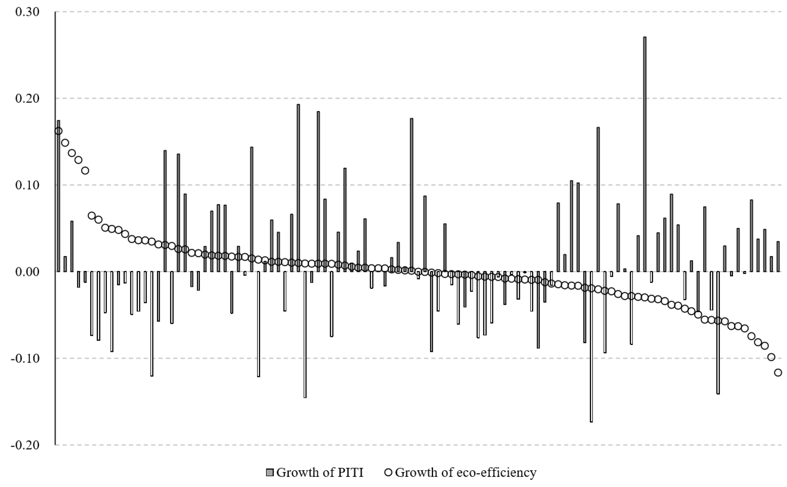
Incorporating metafrontier technique, undesirable outputs and super efficiency into SBM simultaneously, the eco-efficiency is evaluated across each prefecture-level city in China and for each year. We calculate the average change rates of eco-efficiency and PITI over the analyzed period using the geometrical mean, as depicted in Figure 3, indicating that higher growth rate of PITI is not always accompany with higher growth rate of eco-efficiency. On average, the eco-efficiency of the eastern region is the highest (0.5178), followed by western (0.4617) and that of the central is the lowest (0.4491). One possible explanation is that, the industrial structure in central/western region is mainly based on heavy industry; along with the large consumption of coal, energy and other resources, more industrial pollutants will also be produced, resulting in lower eco-efficiency in central/western region. Consequently, the efficiency gap between the eastern and central regions is far greater than that of the central and western regions.
The time evolution of eco-efficiency scores in different regions are illustrated in Figure 4. As shown in the graph, we can conclude that the distribution layout of eco-efficiency for three regions is similar to that of national level, following left skewed distributions as well as having a cluster around 0.4. The vertical lines in Figure 4 show the average eco-efficiency in the corresponding years, indicating that the mean of eco-efficiency for western region decreased significantly from 2008 to 2015. Moreover, the kernel density curves have obviously moved upward over time; as a result, the eco-efficiency gap among eastern region, central region, and western region has decreased. Besides, the kernel density of eco-efficiency scores has two peaks, located at around 0.4 and 1, respectively. It should be noted that the eco-efficiency of prefecture-level cities in China was relatively high but deteriorated slightly from 2008 to 2015 derived from the kernel density curve shifts from right to left. Despite the similar distribution shapes, eco-efficiency scores of different regions are mainly distributed in in the selected year.
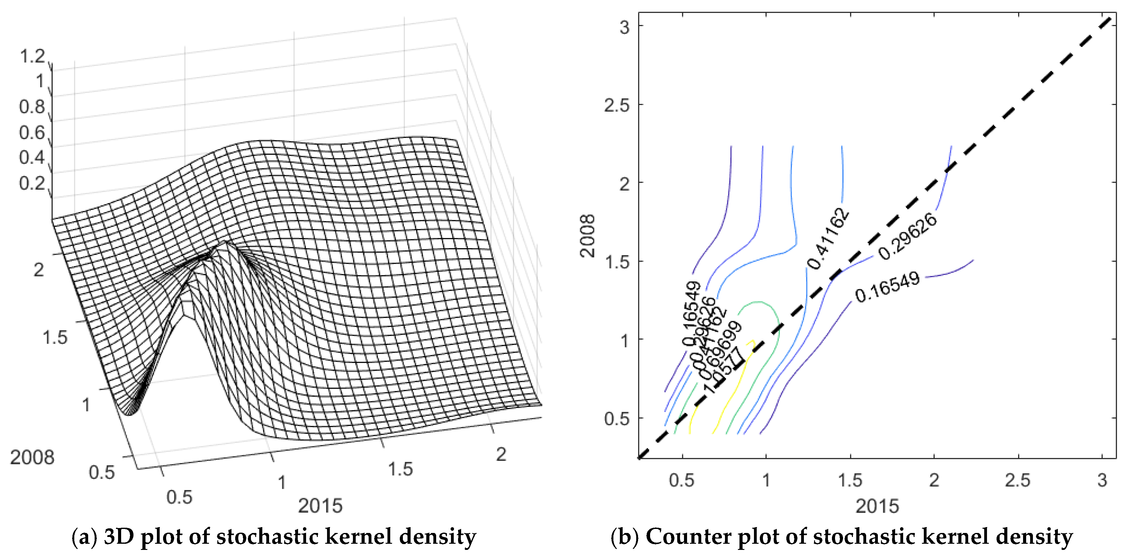
The non-parametric analysis of convergence shows the evolution over time (from time to time ) of eco-efficiency distribution. Figure 5 reports the evolution of eco-efficiency dynamics from 2008 to 2015. The stochastic kernels are calculated by means of a Matlab routine developed by Magrini [52]. The surface plot shows a clear tendency towards a single ridge; moreover, a prominent peak at approximately 1.0577, which lies on the 45° line, can be detected around the middle of the distribution. The stochastic kernel referring to the whole period 2008–2015 shows a strong persistence of eco-efficiency because the kernel is significantly concentrated along the main diagonal, as shown in Figure 5b.
The above findings show that there exist significant regional differences of eco-efficiency in China; exploring the driving forces that impact on eco-efficiency is of importance for policymakers to implement pollution control polices and resource allocation from both theoretical and practical aspects. Thus, it is necessary to investigate the influence factors exert on eco-efficiency using the econometric tools discussed in Section 2.3, and the estimation results are presented in next subsection.
4.2. Estimation Results
4.2.1. Statistical Tests of Unit Root and Granger Causality
To examine the stationarity of the panel data and avoid spurious regressions, along with ensuring the effectiveness of the estimated results, we conduct the panel unit root test on each variable with the Levin–Lin–Chiu (LLC) approach [53]. Table 3 presents the LLC statistics for all the variables at levels. Two model specifications, one with only the intercept and the other with both the intercept and trend, are considered. Results show that all the variables are found to be stationary at levels. Additionally, results of both panel Granger causality [54] and bootstrap Granger causality [55,56] implied that Granger causal relationships run from PITI and PITI2 to EE rather than bi-directionally among PITI, PITI2 and EE in China. Thus, it is rational to further investigate the impact of PITI on eco-efficiency.
4.2.2. Estimation Results of OLS and Quantile Regression
In this section, we investigate the relationship between PITI and eco-efficiency and discuss the estimation results of the present study. First, Figure 6 shows the scatter plot of PITI and eco-efficiency during 2008–2015, along with the nonlinear fitted curve and the confidence interval with confidence level at 95%, illustrating the significant inverted-U-shaped relationship between PITI and eco-efficiency. Then, before the empirical estimates, we perform the Hausman test to select between fixed and random effects models. The significant test statistics and small p-value suggest that fixed effects are more suitable for our empirical models.
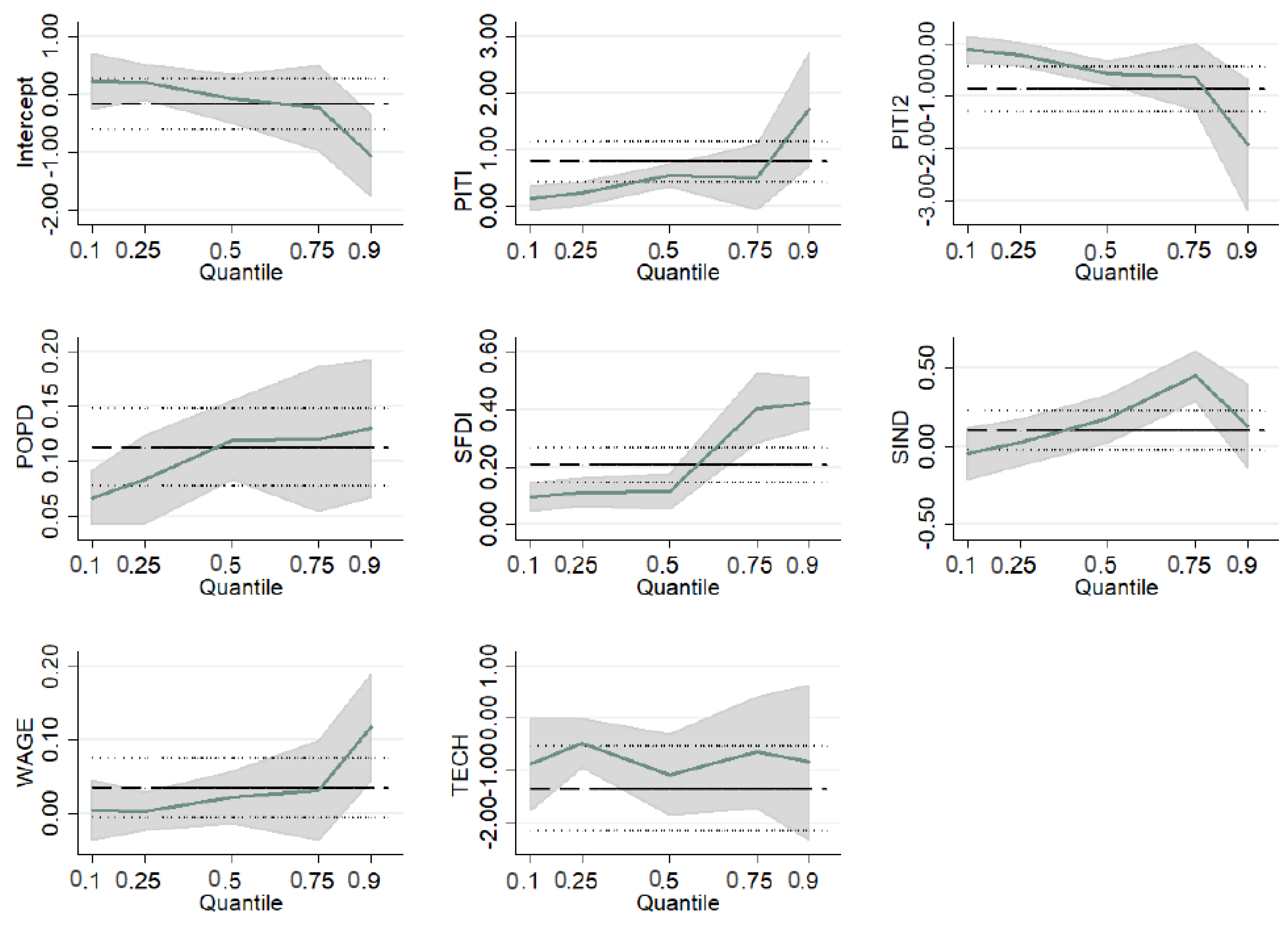
Estimation results of OLS and quantile regression in Table 4 show that PITI is significantly and positively associated with eco-efficiency, while PITI2 is significantly and negatively associated with eco-efficiency. In line with our theoretical predictions, there exist an inverted-U-shaped relation between PITI and eco-efficiency. Furthermore, we found that POPD exerts significant and positive impact on eco-efficiency, e.g., a unit increase in POPD would results in an increase in eco-efficiency score by 0.4364 for FE model, reducing to 0.1129 in pool OLS model, ceteris paribus. As suggested by Ciccone and Hall [57], compared to market scale and urban size, population density is more suitable for measuring regional economic agglomeration. That is, the improvement of eco-efficiency benefits from the promotion of economic agglomeration. Both the linear and quadratic terms of PITI are significant at the 10th, 75th, and 90th quantiles, implying that the inverted-U relationship is only significant around the low and high level of the distribution. Further insights into this result can be obtained by calculating the turning points. In Table 5, we find that the turning points obtained from quantile regression are generally greater than those obtained from FE model which shows that the eco-efficiency will continually increase until PITI reaches its scale of 0.3505.
Figure 7 illustrates the coefficients and bootstrap confidence intervals (draws = 2000) of quantile regression model, indicating that the key interest explanatory variables PITI and PITI2 are positively and negatively associated with eco-efficiency across different quantiles we considered, respectively.
4.2.3. Estimation Results of Spatial Durbin Model
Besides the non-spatial econometric evidence, we investigate the spatial dependence of the regression variables with two standard spatial autocorrelation tests of Moran’s I [58] and Geary’s C [59]. Regarding the ID-EB (inverse distance and economic-based) matrix, for example, the Moran’s I statistic shows that, except for SIND, all variables are spatially autocorrelated at 5% significance while Geary’s C rejects the null hypothesis of spatial independence for most variables, indicating the necessity to use spatial econometric models for further analysis. We then use Lagrange multiplier (LM) tests and their robust versions [37] to choose the most proper spatial econometric model to describe the quantitative relationship among data, along with the SDM generalizes both the spatial lag and the spatial error model, we estimate the SDM finally.
As can be seen in Table 6, with different spatial weight matrix, the coefficients of PITI and PITI2 are significantly positively and negatively associated with eco-efficiency, respectively. Hence, we can argue that there is strong evidence of inverted-U relation between PITI and eco-efficiency of study sample in China. In addition, the spatial coefficients (ρ) are also highly significant, which indicates a strong evidence of spatiality. In Table 6, we use Akaike Information Criterion and Bayesian Information Criterion (AIC and BIC, respectively) to compare goodness of fit for the models, although criteria are mainly aimed at selecting a parsimonious model rather than the model with the most support from the data [60]. Moreover, the coefficients of POPD and WAGE in spatial models are also significantly and positively associated with eco-efficiency, while the coefficients of SFDI are significantly and negatively associated with eco-efficiency. Our results are consistent with [61] and indicate the specification of the spatial weights matrices should have no effect on the estimation results.
Table 7 reports the direct, indirect, and total effects of corresponding models estimated in Table 6. The direct effects of PITI and PITI2 are significantly positive and negative, indicating the beneficial effects of PITI to promote eco-efficiency of host region. In terms of magnitude, a 1% increase in PITI results in an approximate 0.2% increase in eco-efficiency, while a 1% increase in PITI2 results in an approximate 0.3% decrease in eco-efficiency. The indirect effects of PITI and PITI2 are negative and positive, implying the increase in PITI of adjacent cities will lead to reduce eco-efficiency of local city. Among all control variables, POPD and WAGE have significantly positive direct effects on eco-efficiency, hinting that a higher population density and wage level may result in high eco-efficiency to local cities, implying the existence of agglomeration effect and technique effect. In contrast, SFDI and SIND generate negative direct effects on eco-efficiency, implying the existence of composition effect. In Table 8, we find that the turning points obtained from the SDM are generally smaller than those obtained from FE and quantile regression models, showing that the eco-efficiency will continually increase till PITI approximately reaches its scale of 0.34.
4.2.4. Supplementary Analysis: Panel Threshold Model
Given the presumed thresholds in a nonlinear relation, the pollution information transparency index (PITI) for a city may have different influences on eco-efficiency in that city above and below those thresholds. For supplementary analysis, we built a threshold model [62] as follows:
where is the assumed specific threshold value and is defined as an indicator function.
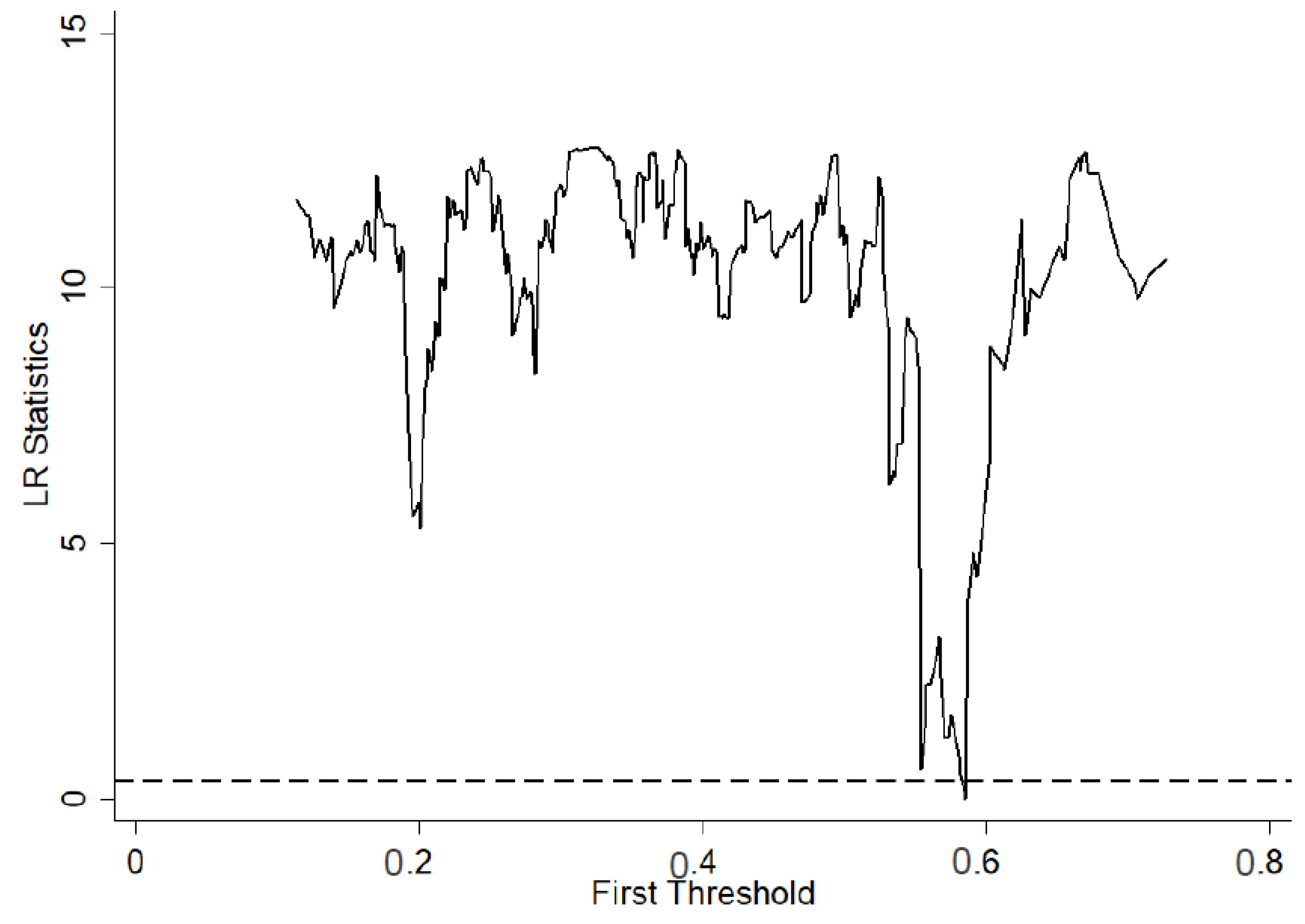
Table 9 reports the testing for both single and double threshold effects. The F-statistics and p-values tested indicated an extremely insignificant relation between the two threshold values assumed, indicating the 100% rejection of the hypothesis that there are no two-threshold values. Figure 8 illustrates the LR statistics for testing single threshold effects. According to the threshold test results, there is a nonlinear relation between PITI and eco-efficiency, instead of a linear and positive assumption between PITI and eco-efficiency; particularly, the eco-efficiency will continually increase until PITI reaches its scale of 0.5850.
5. Conclusions
We explore empirically the effect of environmental disclosure measured by pollution information transparency index (PITI) on eco-efficiency using a dataset for 109 key environmental protection (KEP) prefecture-level cities in China during 2008–2015. Meta-US-SBM model, quantile regression, and the SDM are applied throughout the paper. The main conclusions and corresponding policy implications are summarized as follows:
(1) Results of DEA model shows that there exist significant spatiotemporal disparities of eco-efficiency; on average, the eco-efficiency in eastern region is relatively higher than central/western region. To reduce the efficiency gap, the links between different regions should be strengthened so the eco-efficiency can be promoted in a coordinated way by improving industrial agglomeration and optimizing the resources allocation.
(2) Bootstrap Granger causality test implied that there exist unidirectional Granger causal relationships running from PITI and PITI2 to EE rather than bidirectional relationships among PITI, PITI2 and EE in China. Thus, it is of importance to pay high attention to environmental information disclosure in the process of ecological civilization in China.
(3) Both OLS and quantile regression show that the evidence of an inverted-U-shaped relation between PITI and eco-efficiency is supported, and the turning points range from 0.3505 to 0.4540. Estimation results of the SDM also support this finding, and the turning points become relatively smaller after considering spatial effects, varying from 0.3370 to 0.3542 based on different specifications of spatial weights matrices. Furthermore, improving and upgrading the levels of agglomeration, wages and technology will contribute to the promotion of eco-efficiency, while the industrial structure should be readjusted and optimized energetically.
(4) Panel threshold model also shows that the existence threshold effect between PITI and eco-efficiency, providing evidence that the eco-efficiency will continually increase until PITI reaches its threshold value.
Due to data restrictions, the period covered in this study was only eight years. Therefore, future studies can be conducted from three aspects. First, the time span can be increased to cover a longer period, and more information and data can be used to analyze the eco-efficiency of China, such as convergence analysis. Second, more precise measurement of environmental disclosure can be aggregated by micro-level datum. Third, the proposed DEA model can be extended to measure and compare productivity changes for prefecture-level cities in different groups under the framework of the Malmquist–Luenberger productivity indicator. With the same metafrontier, these indicators are comparable and can provide insightful information. Furthermore, to relax the assumption of a linear relationship on both sides of the threshold, panel smooth transition regression (PSTR) model should be adopted to empirically study the nonlinear relationship between PITI and eco-efficiency.
Acknowledgments
The authors wish to thank the three anonymous referees for valuable comments on the early drafts of this paper. All remaining errors are the authors’. This research is supported by the National Natural Science Foundation of China (Grant No. 41571524) and the Major Program of the National Social Science Foundation of China (Grant No. 11&ZD012 and Grant No. 17ZDA081).
Author Contributions
Yantuan Yu and Jianhuan Huang had the initial idea for the study. Yantuan Yu is responsible for the data collection and econometric analysis. Nengsheng Luo proofread the paper. All authors have read and approved the final manuscript.
Conflicts of Interest
The authors declare no conflict of interest.
Appendix A. List of 109 KEP Cities Included into the Sample

Table A1.
The 109 KEP cities.
| Region | City | Region | City | Region | City |
|---|---|---|---|---|---|
| Eastern (49) | Jining | Changsha | |||
| Beijing Municipality | Tai’an | Zhuzhou | |||
| Tianjin Municipality | Rizhao | Xiangtan | |||
| Shijiazhuang | Guangzhou | Yueyang | |||
| Tangshan | Shaoguan | Changde | |||
| Qinhuangdao | Shenzhen | Zhangjiajie | |||
| Handan | Zhuhai | Western (29) | |||
| Baoding | Shantou | Hohhot | |||
| Shenyang | Foshan | Baotou | |||
| Dalian | Zhanjiang | Chifeng | |||
| Anshan | Dongguan | Nanning | |||
| Fushun | Zhongshan | Liuzhou | |||
| Benxi | Central (31) | Guilin | |||
| Shanghai Municipality | Taiyuan | Beihai | |||
| Nanjing | Datong | Chongqing Municipality | |||
| Wuxi | Yangquan | Chengdu | |||
| Xuzhou | Changzhi | Panzhihua | |||
| Changzhou | Linfen | Luzhou | |||
| Suzhou | Changchun | Mianyang | |||
| Nantong | Jilin | Yibin | |||
| Lianyungang | Harbin | Guiyang | |||
| Yangzhou | Qiqihar | Zunyi | |||
| Hangzhou | Daqing | Kunming | |||
| Ningbo | Mudanjiang | Qujing | |||
| Wenzhou | Hefei | Xi’an | |||
| Jiaxing | Wuhu | Tongchuan | |||
| Huzhou | Maanshan | Baoji | |||
| Shaoxing | Nanchang | Xianyang | |||
| Taizhou | Jiujiang | Yan’an | |||
| Fuzhou | Zhengzhou | Lanzhou | |||
| Xiamen | Kaifeng | Jinchang | |||
| Quanzhou | Luoyang | Xi’ning | |||
| Jinan | Pingdingshan | Yichuan | |||
| Qingdao | Anyang | Shizuishan | |||
| Zibo | Jiaozuo | Urumqi | |||
| Zaozhuang | Wuhan | Karamay | |||
| Yantai | Yichang | ||||
| Weifang | Jingzhou | ||||
Appendix B. Computation of Environmental Pollution Index
Following Bian and Yang [47] and Ludovisi [48], we construct a composite environmental pollution index (EPI) using the entropy to measure the weights of each pollutants, which helps to alleviate the influence of extreme values of individual factors. The calculation process involves four steps.
Let denote the emission volume of pollutant at region in year . This is first normalized over entire sample:
The entropy of pollutant at region is defined as:
Next, we calculate the weight of pollutant at region as:
The composite environmental pollution index (EPI) covering four pollutants of region in year is given by:
Higher EPI indicates higher level of environmental pollution.
Appendix C. Data Sources
Table A2.
Data sources of DEA model and econometric model.
| Variable | Sources | |
| DEA model | Labor | China City Statistical Yearbook |
| Capital | China City Statistical Yearbook and China Statistical Yearbook | |
| Land | China City Statistical Yearbook | |
| Energy | GDP energy intensity (manually collected from various official documents) multiplied by GDP, China Energy Statistical Yearbook | |
| GDP | China City Statistical Yearbook | |
| EPI | China City Statistical Yearbook and China Environment Yearbook | |
| Econometric model | EE | Measured by Model (4) |
| PITI | Institute of Public & Environmental Affairs and Natural Resource Defense Council (2008–2016) | |
| PITI2 | Quadratic term of PITI | |
| POPD | China City Statistical Yearbook | |
| SFDI | China City Statistical Yearbook | |
| SIND | China City Statistical Yearbook | |
| WAGE | China City Statistical Yearbook | |
| TECH | China City Statistical Yearbook |
References
- Schaltegger, S.; Sturm, A. Ökologische Rationalität: Ansatzpunkte zur Ausgestaltung von ökologieorientierten Managementinstrumenten. Die Unternehmung 1990, 44, 273–290. [Google Scholar]
- Huang, J.; Xia, J.; Yu, Y.; Zhang, N. Composite eco-efficiency indicators for China based on data envelopment analysis. Ecol. Indic. 2018, 85, 674–697. [Google Scholar] [CrossRef]
- Lehni, M. Eco-Efficiency: Creating More Value with Less Impact; World Business Center for Sustainable Development: Geneva, Switzerland, 2000. [Google Scholar]
- Mickwitz, P.; Melanen, M.; Rosenström, U.; Seppälä, J. Regional eco-efficiency indicators-a participatory approach. J. Clean. Prod. 2006, 14, 1603–1611. [Google Scholar] [CrossRef]
- Zhang, B.; Bi, J.; Fan, Z.; Ge, J. Eco-efficiency analysis of industrial system in China: A data envelopment analysis approach. Ecol. Econ. 2008, 68, 306–316. [Google Scholar] [CrossRef]
- Huppes, G.; Ishikawa, M. A Framework for Quantified Eco-efficiency Analysis. J. Ind. Ecol. 2010, 9, 25–41. [Google Scholar] [CrossRef]
- Picazo-Tadeo, A.J.; Gómez-Limón, J.A.; Reig-Martínez, E. Assessing farming eco-efficiency: A data envelopment analysis approach. J. Environ. Manag. 2011, 92, 1154–1164. [Google Scholar] [CrossRef] [PubMed]
- Huang, J.; Yang, X.; Cheng, G.; Wang, S. A comprehensive eco-efficiency model and dynamics of regional eco-efficiency in China. J. Clean. Prod. 2014, 67, 228–238. [Google Scholar] [CrossRef]
- Zhang, N.; Kong, F.; Yu, Y. Measuring ecological total-factor energy efficiency incorporating regional heterogeneities in China. Ecol. Indic. 2015, 51, 165–172. [Google Scholar] [CrossRef]
- Arabi, B.; Munisamy, S.; Emrouznejad, A.; Toloo, M.; Ghazizadeh, M.S. Eco-efficiency considering the issue of heterogeneity among power plants. Energy 2016, 111, 722–735. [Google Scholar] [CrossRef]
- Masternak-Janus, A.; Rybaczewska-Błażejowska, M. Comprehensive Regional Eco-Efficiency Analysis Based on Data Envelopment Analysis: The Case of Polish Regions. J. Ind. Ecol. 2017, 21, 180–190. [Google Scholar] [CrossRef]
- Al-Tuwaijri, S.A.; Christensen, T.E.; Ii, K.E.H. The relations among environmental disclosure, environmental performance, and economic performance: A simultaneous equations approach. Account. Org. Soc. 2004, 29, 447–471. [Google Scholar] [CrossRef]
- Clarkson, P.M.; Li, Y.; Richardson, G.D.; Vasvari, F.P. Revisiting the relation between environmental performance and environmental disclosure: An empirical analysis. Account. Org. Soc. 2008, 33, 303–327. [Google Scholar] [CrossRef]
- Cho, C.H.; Patten, D.M. The role of environmental disclosures as tools of legitimacy: A research note. Account. Org. Soc. 2007, 32, 639–647. [Google Scholar] [CrossRef]
- Villiers, C.D.; van Staden, C.J. Can less environmental disclosure have a legitimising effect? Evidence from Africa. Account. Org. Soc. 2006, 31, 763–781. [Google Scholar] [CrossRef]
- Berthelot, S.; Cormier, D.; Magnan, M. Environmental disclosure research: Review and synthesis. J. Account. Lit. 2003, 22, 1–44. [Google Scholar]
- Liu, Z.G.; Liu, T.T.; McConkey, B.G.; Li, X. Empirical analysis on environmental disclosure and environmental performance level of listed steel companies. Energy Procedia 2011, 5, 2211–2218. [Google Scholar] [CrossRef]
- Sutantoputra, A.W.; Lindorff, M.; Johnson, E.P. The relationship between environmental performance and environmental disclosure. Australas. J. Environ. Manag. 2012, 19, 51–65. [Google Scholar] [CrossRef]
- Zhang, L.; Mol, A.P.J.; He, G. Transparency and information disclosure in China’s environmental governance. Curr. Opin. Environ. Sustian. 2016, 18, 17–24. [Google Scholar] [CrossRef]
- Li, Z.; Ouyang, X.; Du, K.; Zhao, Y. Does government transparency contribute to improved eco-efficiency performance? An empirical study of 262 cities in China. Energy Policy 2017, 110, 79–89. [Google Scholar] [CrossRef]
- Yook, K.H.; Song, H.; Patten, D.M.; Kim, I.W. The disclosure of environmental conservation costs and its relation to eco-efficiency: Evidence from Japan. Sustian. Account. Manag. Policy J. 2017, 8, 20–42. [Google Scholar] [CrossRef]
- Darrell, W.; Schwartz, B.N. Environmental disclosures and public policy pressure. J. Account. Public Policy 1997, 16, 125–154. [Google Scholar] [CrossRef]
- Tilling, M.V. Some thoughts on legitimacy theory in social and environmental accounting. Soc. Environ. Account. J. 2004, 24, 3–7. [Google Scholar] [CrossRef]
- Wei, Q.; Schaltegger, S. Revisiting carbon disclosure and performance: Legitimacy and management views. Br. Account. Rev. 2017, 49, 365–379. [Google Scholar]
- Hummel, K.; Schlick, C. The relationship between sustainability performance and sustainability disclosure—Reconciling voluntary disclosure theory and legitimacy theory. J. Account. Public Policy 2016, 35, 455–476. [Google Scholar] [CrossRef]
- Battese, G.E.; Rao, D.S.P.; O’Donnell, C.J. A metafrontier production function for estimation of technical efficiencies and technology gaps for firms operating under different technologies. J. Prod. Anal. 2004, 21, 91–103. [Google Scholar] [CrossRef]
- Andersen, P.; Petersen, N.C. A procedure for ranking efficient units in data envelopment analysis. Manag. Sci. 1993, 39, 1261–1264. [Google Scholar] [CrossRef]
- Wang, A. Explaining Environmental Information Disclosure in China. Ecol. Law Q. 2017–2018, 44. Forthcoming; UCLA School of Law, Public Law Research Paper No. 17-14. Available online: https://ssrn.com/abstract=2956069 (accessed on 20 April 2017).
- Koenker, R.; Bassett, G., Jr. Regression quantiles. Econometrica 1978, 46, 33–50. [Google Scholar] [CrossRef]
- Canay, I.A. A simple approach to quantile regression for panel data. Econ. J. 2011, 14, 368–386. [Google Scholar] [CrossRef]
- Zhang, Y.J.; Peng, H.R.; Liu, Z.; Tan, W. Direct energy rebound effect for road passenger transport in China: A dynamic panel quantile regression approach. Energy Policy 2015, 87, 303–313. [Google Scholar] [CrossRef]
- Rejeb, A.B.; Arfaoui, M. Financial market interdependencies: A quantile regression analysis of volatility spillover. Res. Int. Bus. Financ. 2016, 36, 140–157. [Google Scholar] [CrossRef]
- Moutinho, V.; Madaleno, M.; Robaina, M. The economic and environmental efficiency assessment in EU cross-country: Evidence from DEA and quantile regression approach. Ecol. Indic. 2017, 78, 85–97. [Google Scholar] [CrossRef]
- Agyiretettey, F.; Ackah, C.G.; Asuman, D. An Unconditional Quantile Regression Based Decomposition of Spatial Welfare Inequalities in Ghana. J. Dev. Stud. 2017, 1–20. [Google Scholar] [CrossRef]
- Anselin, L. Lagrange multiplier test diagnostics for spatial dependence and spatial heterogeneity. Geogr. Anal. 1988, 20, 1–17. [Google Scholar] [CrossRef]
- LeSage, J.P. An Introduction to Spatial Econometrics; Revue D’économie Industrielle; CRC Press: Boca Raton, FL, USA, 2008; pp. 19–44. [Google Scholar]
- Elhorst, J.P. Spatial Econometrics: From Cross-Sectional Data to Spatial Panels; Springer Brief in Regional Science; Springer: Berlin/Heidelberg, Germany, 2014. [Google Scholar]
- Halleck Vega, S.; Elhorst, J.P. The SLX model. J. Reg. Sci. 2015, 55, 339–363. [Google Scholar] [CrossRef]
- Case, A.C.; Rosen, H.S.; Hines, J.R. Budget spillovers and fiscal policy interdependence: Evidence from the states. J. Public Econ. 1993, 52, 285–307. [Google Scholar] [CrossRef]
- Fredriksson, P.G.; Millimet, D.L. Strategic interaction and the determination of environmental policy across US states. J. Urban Econ. 2002, 51, 101–122. [Google Scholar] [CrossRef]
- Lv, Z.; Xu, T. A panel data quantile regression analysis of the impact of corruption on tourism. Curr. Issues Tour. 2016, 20, 1–14. [Google Scholar] [CrossRef]
- CEY. China Environment Yearbooks; China Environment Yearbook Press: Beijing, China, 2005–2016. [Google Scholar]
- CESY. China Energy Statistical Yearbooks; China Statistics Press: Beijing, China, 2005–2016.
- CCSY. China City Statistical Yearbooks; China Statistics Press: Beijing, China, 2005–2016.
- Huang, J.; Yu, Y.; Ma, C. Energy Efficiency Convergence in China: Catch-Up, Lock-In and Regulatory Uniformity. Environ. Resour. Econ. 2017, 1–24. [Google Scholar] [CrossRef]
- Asmild, M.; Zhu, M. Controlling for the use of extreme weights in bank efficiency assessments during the financial crisis. Eur. J. Oper. Res. 2016, 251, 999–1015. [Google Scholar] [CrossRef]
- Bian, Y.; Yang, F. Resource and environment efficiency analysis of provinces in China: A DEA approach based on Shannon’s entropy. Energy Policy 2010, 38, 1909–1917. [Google Scholar] [CrossRef]
- Ludovisi, A. Effectiveness of entropy-based functions in the analysis of ecosystem state and development. Ecol. Indic. 2014, 36, 617–623. [Google Scholar] [CrossRef]
- Zhang, J. Estimation of China’s provincial capital stock (1952-2004) with applications. J. Chin. Econ. Bus. Stud. 2008, 6, 177–196. [Google Scholar] [CrossRef]
- Berlemann, M.; Wesselhöft, J.E. Estimating aggregate capital stocks using the perpetual inventory method. Rev. Econ. 2014, 65, 1–34. [Google Scholar] [CrossRef]
- Ke, S.; Xiang, J. Estimation of the Fixed Capital Stocks in Chinese Cities for 1996-2009. Stat. Res. 2012, 29, 1–10. (In Chinese) [Google Scholar]
- Magrini, S. Analysing Convergence through the Distribution Dynamics Approach: Why and How; Working Paper Number 13/WP/2007; Department of Economics Ca’Foscari, University of Venice: Venice, Italy, 2007. [Google Scholar]
- Levin, A.; Lin, C.F.; Chu, C.S.J. Unit root tests in panel data: Asymptotic and finite-sample properties. J. Econ. 2002, 108, 1–24. [Google Scholar] [CrossRef]
- Granger, C.W.J.; Huang, L.L. Evaluation of Panel Data Models: Some Suggestions from Time Series; Department of Economics, University of California: San Diego, CA, USA, 1997; 29p. [Google Scholar]
- Emirmahmutoglu, F.; Kose, N. Testing for Granger causality in heterogeneous mixed panels. Econ. Model. 2011, 28, 870–876. [Google Scholar] [CrossRef]
- Fang, Z.; Chen, Y. Human capital and energy in economic growth-Evidence from Chinese provincial data. Energy Econ. 2017, 68, 340–358. [Google Scholar] [CrossRef]
- Ciccone, A.; Hall, R.E. Productivity and the density of economic activity. Am. Econ. Rev. 1996, 86, 54–70. [Google Scholar]
- Moran, P.A.P. Notes on continuous stochastic phenomena. Biometrika 1950, 37, 17–23. [Google Scholar] [CrossRef] [PubMed]
- Geary, R.C. The contiguity ratio and statistical mapping. Inc. Stat. 1954, 5, 115–146. [Google Scholar] [CrossRef]
- Qian, S.S. Ecological threshold and environmental management: A note on statistical methods for detecting thresholds. Ecol. Indic. 2014, 38, 192–197. [Google Scholar] [CrossRef]
- LeSage, J.P.; Pace, R.K. The Biggest Myth in Spatial Econometrics. Econometrics 2014, 2, 217–249. [Google Scholar] [CrossRef]
- Hansen, B.E. Threshold effects in non-dynamic panels: Estimation, testing, and inference. J. Econ. 1999, 93, 345–368. [Google Scholar] [CrossRef]
Figure 1.
Total amount of pollution monitoring records, 2006–2016. Sources: Institute of Public & Environmental Affairs and Natural Resource Defense Council (2016–2017).
Figure 1.
Total amount of pollution monitoring records, 2006–2016. Sources: Institute of Public & Environmental Affairs and Natural Resource Defense Council (2016–2017).

Figure 2.
Methodological steps performed in the empirical analysis.
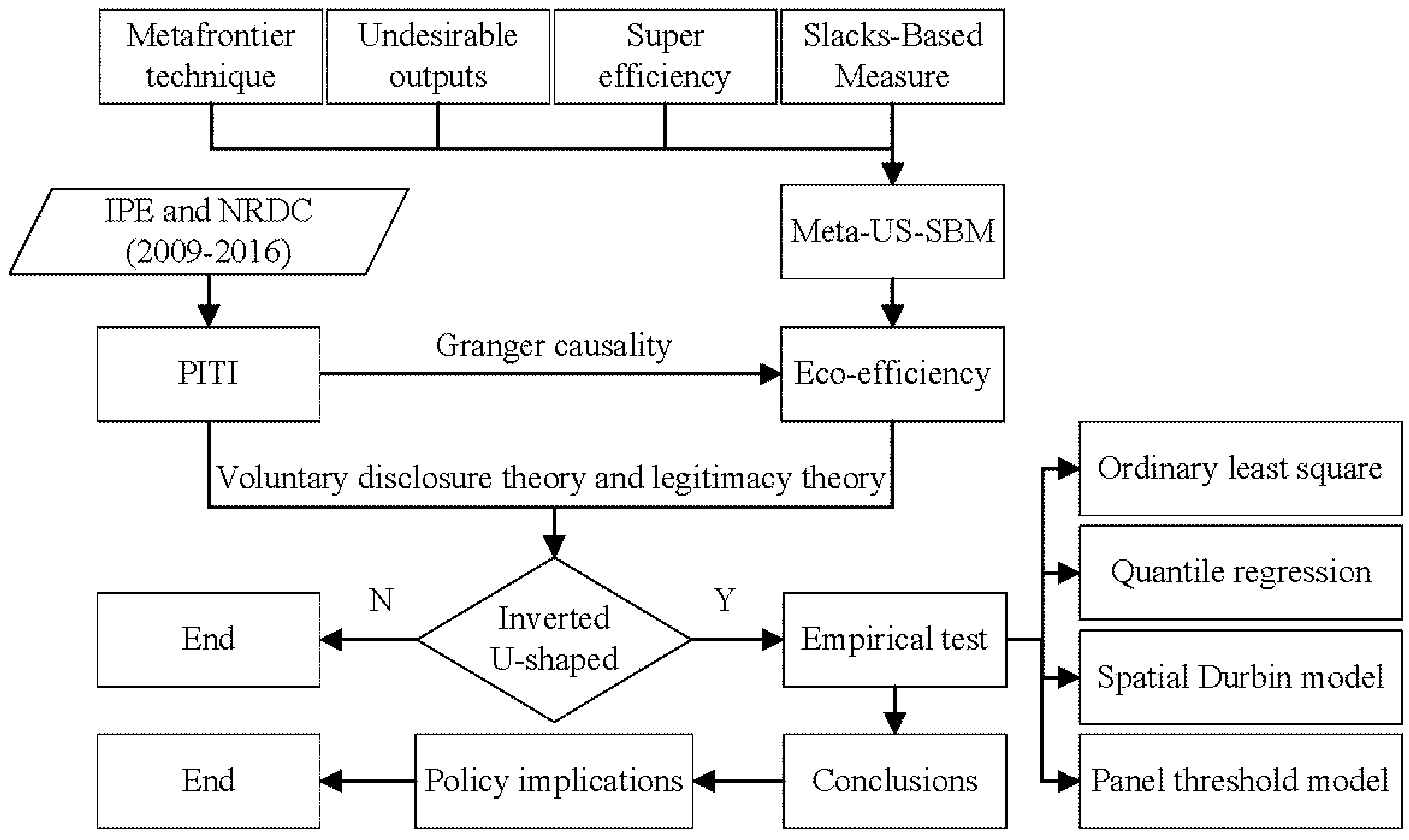
Figure 3.
Prefecture-level cities sorting by growth rate of eco-efficiency, 2008–2015.

Figure 4.
Kernel density estimation of eco-efficiency for different regions.
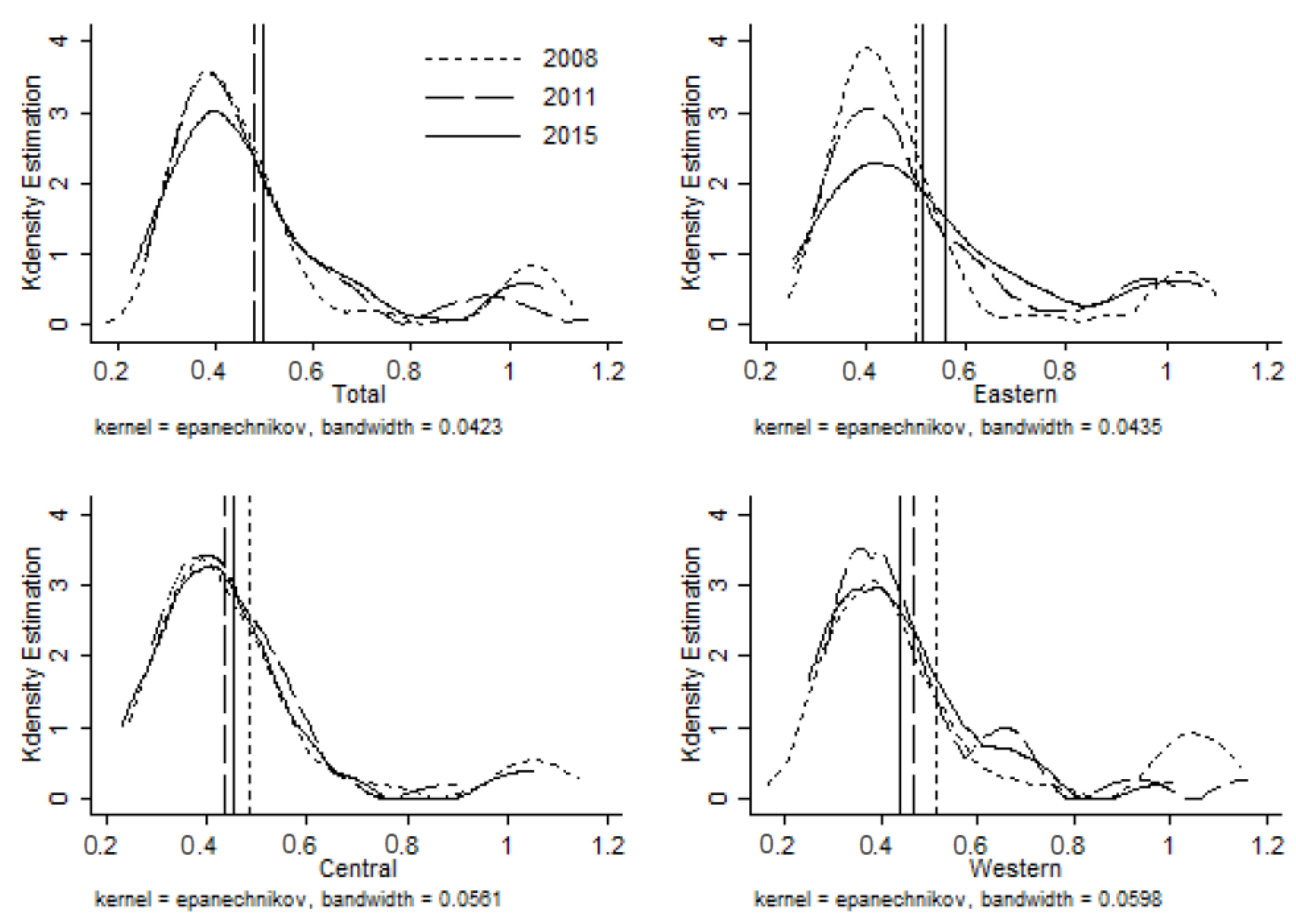
Figure 5.
3D and counter plots of stochastic kernel densities of eco-efficiency from initial period to final period.
Figure 5.
3D and counter plots of stochastic kernel densities of eco-efficiency from initial period to final period.

Figure 6.
Inverted-U-shaped relationship between PITI and eco-efficiency (2008–2015).
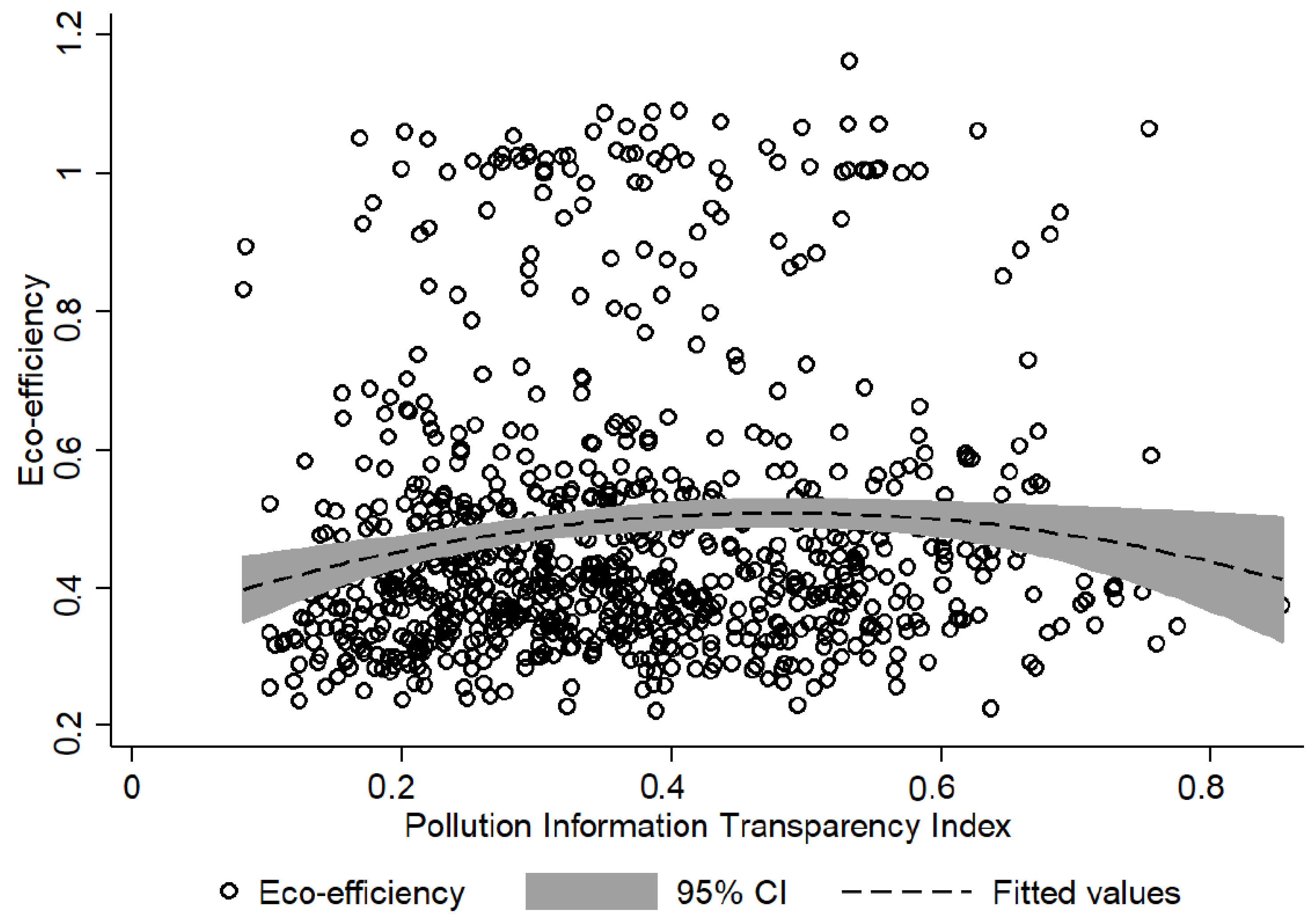
Figure 7.
Coefficients and bootstrap confidence intervals (draws = 2000) of quantile regression.

Figure 8.
Testing for the single threshold effect.

Table 1.
Descriptive statistics.
| Variable | Obs. | Unit | Mean | Std. Dev. | Min | Max | |
|---|---|---|---|---|---|---|---|
| DEA model | Labor | 872 | 10,000 persons | 88.9464 | 107.8553 | 6.7070 | 986.8700 |
| Capital | 872 | 100 million RMB | 2660.0000 | 2740.0000 | 63.6000 | 22,000.0000 | |
| Land | 872 | km2 | 13,820.4800 | 13,256.3700 | 1573.0000 | 90,659.0000 | |
| Energy | 872 | Tons of SCE | 2561.7100 | 1978.5020 | 147.6930 | 11,719.5000 | |
| GDP | 872 | 100 million RMB | 3180.0000 | 3350.0000 | 130.0000 | 25,000.0000 | |
| EPI | 872 | - | 1.1468 | 1.0351 | 0.0993 | 16.8606 | |
| Econometric model | EE | 872 | - | 0.4834 | 0.1999 | 0.2210 | 1.1630 |
| PITI | 872 | - | 0.3680 | 0.1553 | 0.0830 | 0.8530 | |
| PITI2 | 872 | - | 0.1595 | 0.1309 | 0.0069 | 0.7276 | |
| POPD | 872 | 1000 persons/km2 | 0.5456 | 0.3919 | 0.0388 | 2.6481 | |
| SFDI | 872 | - | 0.2002 | 0.2302 | 0.0000 | 1.4432 | |
| SIND | 872 | - | 0.5183 | 0.1012 | 0.1974 | 0.9097 | |
| WAGE | 872 | - | 10.6216 | 0.3189 | 9.6542 | 11.6358 | |
| TECH | 872 | - | 0.0202 | 0.0159 | 0.0016 | 0.0986 |
Table 2.
Correlation coefficients for regression variables.
| EE | PITI | PITI2 | POPD | SFDI | SIND | WAGE | TECH | |
|---|---|---|---|---|---|---|---|---|
| EE | 1.0000 | |||||||
| PITI | 0.0760 ** | 1.0000 | ||||||
| PITI2 | 0.0530 | 0.9770 *** | 1.0000 | |||||
| POPD | 0.3380 *** | 0.0320 | 0.035 | 1.0000 | ||||
| SFDI | 0.3480 *** | 0.0200 | 0.035 | 0.4620 *** | 1.0000 | |||
| SIND | 0.0240 | 0.0330 | 0.033 | −0.1450 *** | −0.0760 ** | 1.0000 | ||
| WAGE | 0.1250 *** | −0.0440 | −0.042 | 0.2060 *** | 0.2620 *** | −0.1550 *** | 1.0000 | |
| TECH | −0.1320 *** | −0.0780 ** | −0.081 ** | −0.0310 | −0.0650 * | −0.2740 *** | 0.2420 *** | 1.0000 |
Note: ***, **, and * denote statistical significance at the 1%, 5%, and 10% significance levels, respectively.
Table 3.
Panel unit root test results.
| Level | ||||
|---|---|---|---|---|
| Intercept | Intercept and Trend | |||
| EE | −0.6969 *** | (−14.2660) | −1.5904 *** | (−59.1930) |
| PITI | −1.1365 *** | (−25.8790) | −1.7020 *** | (−42.6810) |
| PITI2 | −1.1487 *** | (−25.3460) | −1.8994 *** | (−45.2540) |
| POPD | −0.2337 *** | (−13.0780) | −1.3823 *** | (−39.5360) |
| SFDI | −0.3729 *** | (−10.7740) | −1.4691 *** | (−65.3220) |
| SIND | −0.4174 *** | (−22.7920) | −0.6354 *** | (−28.7230) |
| TECH | −0.7564 *** | (−18.9200) | −1.4770 *** | (−38.8110) |
Notes: The maximum lag length to be included in the model is set to 1; *** denotes statistical significance at the 1% significance level; t-statistics are given in the parentheses.
Table 4.
OLS and quantile regression results of model (dependent variable: EE).
| (1) | (2) | (3) | (4) | (5) | (6) | (7) | |
|---|---|---|---|---|---|---|---|
| Variable | Pool OLS | FE | Quantile Regression | ||||
| 10th | 25th | 50th | 75th | 90th | |||
| PITI | 0.7895 *** | 0.1974 ** | 0.1975 *** | 0.0624 | 0.1320 | 0.1915 *** | 1.3186 *** |
| (4.8492) | (2.0427) | (4.7273) | (1.5918) | (1.1037) | (6.7093) | (2.9324) | |
| PITI2 | −0.8701 *** | −0.2816 ** | −0.2633 *** | −0.0937 ** | −0.1389 | −0.2109 *** | −1.6194 *** |
| (−4.5736) | (−2.3647) | (−3.1906) | (−2.0697) | (−0.9986) | (−5.8970) | (−3.0553) | |
| POPD | 0.1129 *** | 0.4364 *** | 0.0776 *** | 0.0526 *** | 0.1500 *** | 0.0719 *** | 0.1049 *** |
| (5.5408) | (2.7121) | (9.3876) | (4.4373) | (5.7884) | (13.3616) | (3.3808) | |
| SFDI | 0.2051 *** | −0.1866 ** | 0.0625 *** | 0.1769 *** | 0.1330 *** | 0.3902 *** | −0.0867 |
| (5.3410) | (−2.2589) | (3.3452) | (23.1193) | (4.2489) | (55.3353) | (−0.6546) | |
| SIND | 0.1025 | −0.1461 | −0.0323 ** | 0.1634 *** | 0.1303 *** | 0.2738 *** | −0.2644 |
| (1.0763) | (−1.0325) | (−2.1717) | (10.0562) | (8.8133) | (11.3106) | (−1.4661) | |
| WAGE | 0.0347 | 0.1563 ** | −0.0016 | −0.0421 *** | 0.0713 *** | 0.0583 *** | 0.3859 ** |
| (1.5854) | (2.5749) | (−0.2175) | (−4.7291) | (3.6603) | (17.6245) | (2.3921) | |
| TECH | −1.3456 *** | 0.8168 | −0.7918 *** | −0.0686 | −0.9622 *** | −1.3632 *** | −4.6986 *** |
| (−3.1873) | (0.6997) | (−4.2873) | (−1.0968) | (−19.6825) | (−19.6231) | (−5.7829) | |
Notes: Robust t-statistics are in parentheses; ***, **, and * denote statistical significance at the 1%, 5%, and 10% significance levels, respectively.
Table 5.
Turning points.
| (1) | (2) | (3) | (4) | (5) | (6) | (7) | |
|---|---|---|---|---|---|---|---|
| Variable | Pool OLS | FE | Quantile Regression | ||||
| 10th | 25th | 50th | 75th | 90th | |||
| PITI * | 0.4537 | 0.3505 | 0.3750 | NA | NA | 0.4540 | 0.4071 |
Note: NA denotes that the results are not available. Superscript * denotes the interested independent variable: pollution information transparency index
Table 6.
Estimation results of Spatial Durbin Model (dependent variable: EE).
| (1) | (2) | (3) | (4) | |||||
|---|---|---|---|---|---|---|---|---|
| Variable | Inverse Distance Matrix | Economic-Based Matrix | Inverse Distance and Economic-Based Matrix | Population-Distance-Based Matrix | ||||
| PITI | 0.1685 * | (1.9046) | 0.2108 ** | (2.4150) | 0.1915 ** | (2.1882) | 0.1691 * | (1.9040) |
| PITI2 | −0.2500 ** | (−2.4171) | −0.2976 *** | (−2.9256) | −0.2748 *** | (−2.6943) | −0.2491 ** | (−2.3989) |
| POPD | 0.4658 *** | (5.5019) | 0.3797 *** | (4.5812) | 0.4106 *** | (4.7467) | 0.4798 *** | (5.6465) |
| SFDI | −0.1813 *** | (−3.2755) | −0.1582 *** | (−2.8477) | −0.1473 *** | (−2.6019) | −0.1818 *** | (−3.2685) |
| SIND | −0.0553 | (−0.4570) | −0.0884 | (−0.8185) | −0.0193 | (−0.1712) | −0.0516 | (−0.4259) |
| WAGE | 0.1757 *** | (4.1175) | 0.1572 *** | (3.7600) | 0.1671 *** | (3.9253) | 0.1753 *** | (4.0813) |
| TECH | 1.4093 * | (1.9363) | 0.6506 | (0.9260) | 0.8236 | (1.1602) | 1.4065* | (1.9320) |
| W*PITI | −1.0690 | (−1.3788) | −0.2906 | (−1.0696) | −0.2466 | (−1.0178) | −1.0073 | (−1.2991) |
| W*PITI2 | 1.2897 | (1.3785) | 0.3217 | (0.9725) | 0.2850 | (0.9861) | 1.2622 | (1.3485) |
| W*POPD | −1.8345 *** | (−3.5051) | 0.9066 *** | (2.8570) | 0.1937 | (0.7843) | −1.6461 *** | (−3.2014) |
| W*SFDI | −1.1522 *** | (−3.0795) | −0.1416 | (−1.1196) | −0.0606 | (−0.4617) | −1.0277 *** | (−2.8493) |
| W*SIND | −0.4715 | (−0.6836) | −0.4337 | (−1.4829) | −0.7373 *** | (−2.7542) | −0.6766 | (−0.9785) |
| W*WAGE | −0.0255 | (−0.0793) | −0.0056 | (−0.0385) | 0.0480 | (0.3938) | 0.1046 | (0.3300) |
| W*TECH | 5.1552 | (0.8568) | 3.1770 | (1.2561) | −1.9314 | (−0.9205) | 4.5939 | (0.7712) |
| ρ | −0.3483 * | (−1.9563) | 0.1666 ** | (2.2582) | 0.1375 ** | (2.1791) | −0.2645 | (−1.5302) |
| R-squared | 0.0191 | 0.0423 | 0.0869 | 0.0099 | ||||
| Log L | 1033.5962 | 1033.4107 | 1029.4746 | 1031.9667 | ||||
| AIC | −2035.1920 | −2034.8210 | −2026.9490 | −2031.9330 | ||||
| BIC | −1958.8600 | −1958.4890 | −1950.6170 | −1955.6010 | ||||
Notes: The z-statistics are given in the parentheses; ***, **, and * denote statistical significance at the 1%, 5%, and 10% significance levels, respectively; Log L: Log likelihood; individual and time fixed effects are included in every model.
Table 7.
Direct, indirect, and total effects of SDM estimation (dependent variable: EE).
| (1) | (2) | (3) | (4) | |||||
|---|---|---|---|---|---|---|---|---|
| Inverse Distance Matrix | Economic-Based Matrix | Inverse Distance and Economic-Based Matrix | Population-Distance-Based Matrix | |||||
| Panel A: Direct effect | ||||||||
| PITI | 0.1800 ** | (1.9871) | 0.2082 ** | (2.3097) | 0.1899 ** | (2.1024) | 0.1783 ** | (1.9622) |
| PITI2 | −0.2649 ** | (−2.5028) | −0.2959 *** | (−2.8088) | −0.2741 *** | (−2.5963) | −0.2616 ** | (−2.4611) |
| POPD | 0.4883 *** | (5.9892) | 0.4090 *** | (5.1280) | 0.4239 *** | (5.1619) | 0.4980 *** | (6.0934) |
| SFDI | −0.1730 *** | (−3.1495) | −0.1614 *** | (−2.9429) | −0.1488 *** | (−2.6799) | −0.1758 *** | (−3.1944) |
| SIND | −0.0507 | (−0.4244) | −0.0969 | (−0.9266) | −0.0335 | (−0.3095) | −0.0465 | (−0.3910) |
| WAGE | 0.1786 *** | (4.2069) | 0.1596 *** | (3.8088) | 0.1704 *** | (4.0470) | 0.1771 *** | (4.1551) |
| TECH | 1.3781* | (1.8308) | 0.7295 | (0.9827) | 0.7914 | (1.0570) | 1.3854 * | (1.8366) |
| Panel B: Indirect effect | ||||||||
| PITI | −0.8717 | (−1.5727) | −0.3108 | (−1.0134) | −0.2591 | (−0.9751) | −0.8677 | (−1.4686) |
| PITI2 | 1.0767 | (1.5856) | 0.3398 | (0.9003) | 0.2974 | (0.9307) | 1.1072 | (1.5275) |
| POPD | −1.4978 *** | (−3.4695) | 1.1562 *** | (3.0592) | 0.2873 | (1.0544) | −1.4168 *** | (−3.1491) |
| SFDI | −0.8237 *** | (−2.8677) | −0.2014 | (−1.4019) | −0.0942 | (−0.6542) | −0.7901 *** | (−2.6734) |
| SIND | −0.3080 | (−0.5611) | −0.4978 | (−1.3436) | −0.8190 ** | (−2.5141) | −0.4961 | (−0.8515) |
| WAGE | −0.0809 | (−0.3491) | 0.0109 | (0.0652) | 0.0703 | (0.5358) | 0.0307 | (0.1265) |
| TECH | 3.5203 | (0.8003) | 4.0135 | (1.3125) | −2.0145 | (−0.8245) | 3.4081 | (0.7318) |
| Panel C: Total effect | ||||||||
| PITI | −0.6918 | (−1.2231) | −0.1026 | (−0.3102) | −0.0693 | (−0.2376) | −0.6894 | (−1.1409) |
| PITI2 | 0.8118 | (1.1691) | 0.0439 | (0.1080) | 0.0234 | (0.0666) | 0.8456 | (1.1385) |
| POPD | −1.0095 ** | (−2.4073) | 1.5652 *** | (4.0387) | 0.7112 *** | (2.6432) | −0.9189 ** | (−2.1030) |
| SFDI | −0.9967 *** | (−3.5217) | −0.3628 ** | (−2.3770) | −0.2429 | (−1.6374) | −0.9659 *** | (−3.2980) |
| SIND | −0.3588 | (−0.7073) | −0.5947 | (−1.5275) | −0.8525 *** | (−2.6199) | −0.5426 | (−1.0005) |
| WAGE | 0.0977 | (0.4248) | 0.1705 | (0.9478) | 0.2407 * | (1.7108) | 0.2079 | (0.8618) |
| TECH | 4.8984 | (1.0756) | 4.7430 | (1.4442) | −1.2231 | (−0.4537) | 4.7935 | (0.9945) |
Notes: The z-statistics are given in the parentheses; ***, **, and * denote statistical significance at the 1%, 5%, and 10% significance levels, respectively.
Table 8.
Estimation results of Spatial Durbin Model (dependent variable: EE).
| (1) | (2) | (3) | (4) | |
|---|---|---|---|---|
| Variable | Inverse Distance Matrix | Economic-Based Matrix | Inverse Distance and Economic-Based Matrix | Population-Distance-Based Matrix |
| PITI * | 0.3370 | 0.3542 | 0.3484 | 0.3394 |
Note: Superscript * represents the interested independent variable: pollution information transparency index
Table 9.
Testing for the threshold effect of PITI on eco-efficiency.
| Test for Single Threshold Effects | Test for Double Threshold Effects | |||||
|---|---|---|---|---|---|---|
| Threshold Values | F | p-Value | Double Threshold Values | F | p-Value | |
| 0.5850 | 12.8600 | 0.0495 | 0.5710 | 0.6030 | 0.2200 | 1.0000 |
Note: The F-statistics and p-value have generated from bootstrap method using 2000 replications.
© 2018 by the authors. Licensee MDPI, Basel, Switzerland. This article is an open access article distributed under the terms and conditions of the Creative Commons Attribution (CC BY) license (http://creativecommons.org/licenses/by/4.0/).
Share and Cite
MDPI and ACS Style
Yu, Y.; Huang, J.; Luo, N. Can More Environmental Information Disclosure Lead to Higher Eco-Efficiency? Evidence from China. Sustainability 2018, 10, 528. https://0-doi-org.brum.beds.ac.uk/10.3390/su10020528
AMA Style
Yu Y, Huang J, Luo N. Can More Environmental Information Disclosure Lead to Higher Eco-Efficiency? Evidence from China. Sustainability. 2018; 10(2):528. https://0-doi-org.brum.beds.ac.uk/10.3390/su10020528
Chicago/Turabian StyleYu, Yantuan, Jianhuan Huang, and Nengsheng Luo. 2018. "Can More Environmental Information Disclosure Lead to Higher Eco-Efficiency? Evidence from China" Sustainability 10, no. 2: 528. https://0-doi-org.brum.beds.ac.uk/10.3390/su10020528
Note that from the first issue of 2016, this journal uses article numbers instead of page numbers. See further details here.