Calibration of a Field-Scale Soil and Water Assessment Tool (SWAT) Model with Field Placement of Best Management Practices in Alger Creek, Michigan

Abstract

Subwatersheds within the Great Lakes “Priority Watersheds” were targeted by the Great Lakes Restoration Initiative (GLRI) to determine the effectiveness of the various best management practices (BMPs) from the U.S. Department of Agriculture-Natural Resources Conservation Service National Conservation Planning (NCP) Database. A Soil and Water Assessment Tool (SWAT) model is created for Alger Creek, a 50 km² tributary watershed to the Saginaw River in Michigan. Monthly calibration yielded very good Nash–Sutcliffe efficiency (NSE) ratings for flow, sediment, total phosphorus (TP), dissolved reactive phosphorus (DRP), and total nitrogen (TN) (0.90, 0.79, 0.87, 0.88, and 0.77, respectively), and satisfactory NSE rating for nitrate (0.51). Two-year validation results in at least satisfactory NSE ratings for flow, sediment, TP, DRP, and TN (0.83, 0.54, 0.73, 0.53, and 0.60, respectively), and unsatisfactory NSE rating for nitrate (0.28). The model estimates the effect of BMPs at the field and watershed scales. At the field-scale, the most effective single practice at reducing sediment, TP, and DRP is no-tillage followed by cover crops (CC); CC are the most effective single practice at reducing nitrate. The most effective BMP combinations include filter strips, which can have a sizable effect on reducing sediment and phosphorus loads. At the watershed scale, model results indicate current NCP BMPs result in minimal sediment and nutrient reductions (<10%).

1. Introduction

The Saginaw River enters Lake Huron through Saginaw Bay, an inlet that has been plagued by algae-related issues ranging from beach closures, to the formation of toxic muck (which threatens human and animal health and degrades beach quality), and to degradation of a freshwater drinking and recreation resource for close to 500,000 people. Nutrient inputs to Saginaw Bay must be managed to control algal blooms that have occurred in recent years [1]. The Saginaw River has been identified as the largest contributor of phosphorus (P) to Lake Huron [2,3], and research currently points to agricultural activities as the main source of nutrients to Saginaw Bay [4].

Water-quality problems have plagued the Great Lakes for decades. Action was taken in the 1970s to reduce contaminants from industry and wastewater treatment facilities, and the 1978 Great Lakes Water Quality Agreement between the United States and Canada established a 440 t year⁻¹ total phosphorus (TP) load as a goal to reduce the algal blooms in Saginaw Bay [5]. Water-quality improvements were seen [6], and in the early 1990s nutrient loads reporting had ceased [7]. The Lakes began to face many new or reoccurring issues (such as areas of concern, algal growth, and invasive species), and the Great Lakes Restoration Initiative (GLRI) was launched in 2010. GLRI is intended to address the many challenges facing the Great Lakes and provides a framework for restoration and protection. The Priority Watersheds Working Group (PWWG) (co-chaired by the U.S. Environmental Protection Agency (EPA) and the U.S. Department of Agriculture-Natural Resources Conservation Service (USDA-NRCS)) focused their efforts on four Priority Watersheds (PWs)—(1) Lower Fox River, Wisconsin; (2) Saginaw River, Michigan; (3) Maumee River, Ohio; and (4) Genesee River, New York—with a goal of reducing the amount of P reaching the Great Lakes from agricultural sources. The PWs were selected due to a high density of agricultural land and the impact caused to their receiving waterbodies [8]. USDA-NRCS is using additional GLRI funding to saturate the PWs with best management practices (BMPs) to help meet the 40% TP reduction goal.

To assess the water-quality impact of the GLRI program, the U.S. Geological Survey (USGS) is participating in the PWWG by providing enhanced monitoring and modeling at the edge-of-field (EOF) and small watershed level. BMP effectiveness is difficult to determine because many factors influence its effectiveness, including, but not limited to, scale, agricultural activity, soils, tile drainage, and weather patterns [9]. Scale is a very important factor concerning nutrient transport, and questions abound on how BMP effectiveness transfers from the field to watershed scale, as many complex processes (landscape, routing, soil interactions, etc.) affect nutrient transport [10]. Most watershed modeling focuses on larger basins, such as the Saginaw River Watershed, and multiple models have been developed for the Saginaw River or Saginaw Bay Watersheds [11,12,13,14]. This modeling effort in the present study was designed to look at a smaller basin—the Alger Creek watershed. A model of a smaller basin allows the user to thoroughly investigate many processes at a smaller scale that would be computationally strained or concealed at a larger scale [15]. The Soil and Water Assessment Tool (SWAT) model was chosen for the work. It has been widely used for assessing the impacts of agricultural management on water quality [16,17,18,19]. In this case, it was configured to have one hydrologic response unit (HRU), where runoff calculations occur, approximately equal to one farm field—similar to the methods presented in Kalcic et al. [20] and Daggupati et al. [21]. This configuration allows for BMPs to be accurately placed, with spatially correct landuse and soils modeled beneath BMPs.

Additionally, the water-quality component of many watershed models are calibrated to only monthly samples or linear regression of monthly samples and daily streamflow [22]. These grab samples are often discontinued during the winter months, and this practice can underestimate the nutrient load [23]. Year-round daily monitoring supports the current modeling effort at the EOF and Alger Creek outlets.

This paper presents a unique effort led by the USGS, as part of the PWWG, at the EOF and small watershed scale. The objectives of this paper are to: (1) describe the calibration and validation for the Alger Creek, Michigan SWAT model; (2) identify critical source areas with the highest runoff, erosion, and nutrient loss potential; (3) estimate the impact EPA GLRI BMPs have on nutrient yields in the Alger Creek watershed; and (4) simulate the influence additional levels of BMP implementation would have on nutrient yields through modeling scenarios. Results will be used by stakeholders to help prioritize and target future GLRI phosphorous reduction efforts. Model limitations also are investigated and described.

2. Materials and Methods

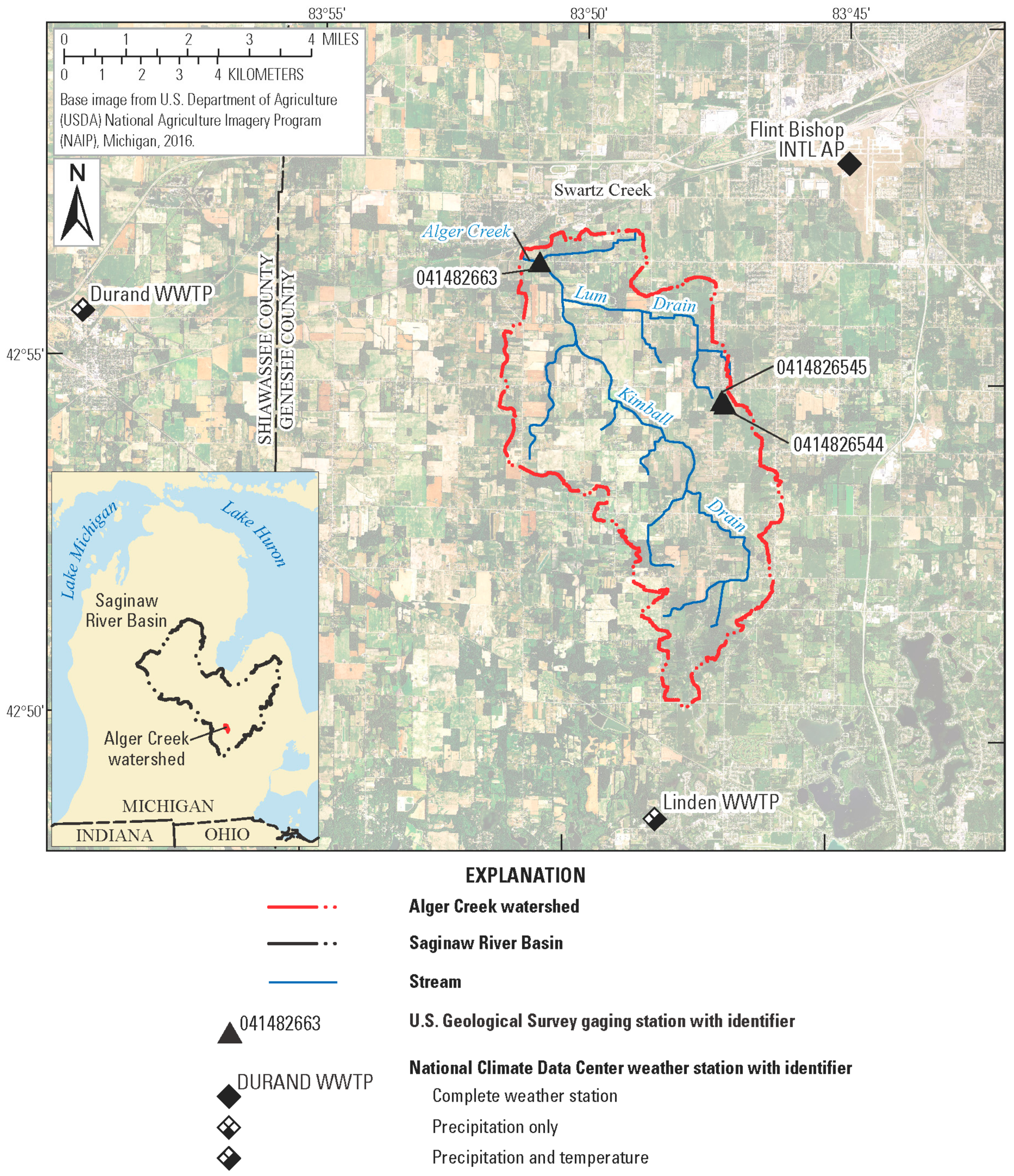
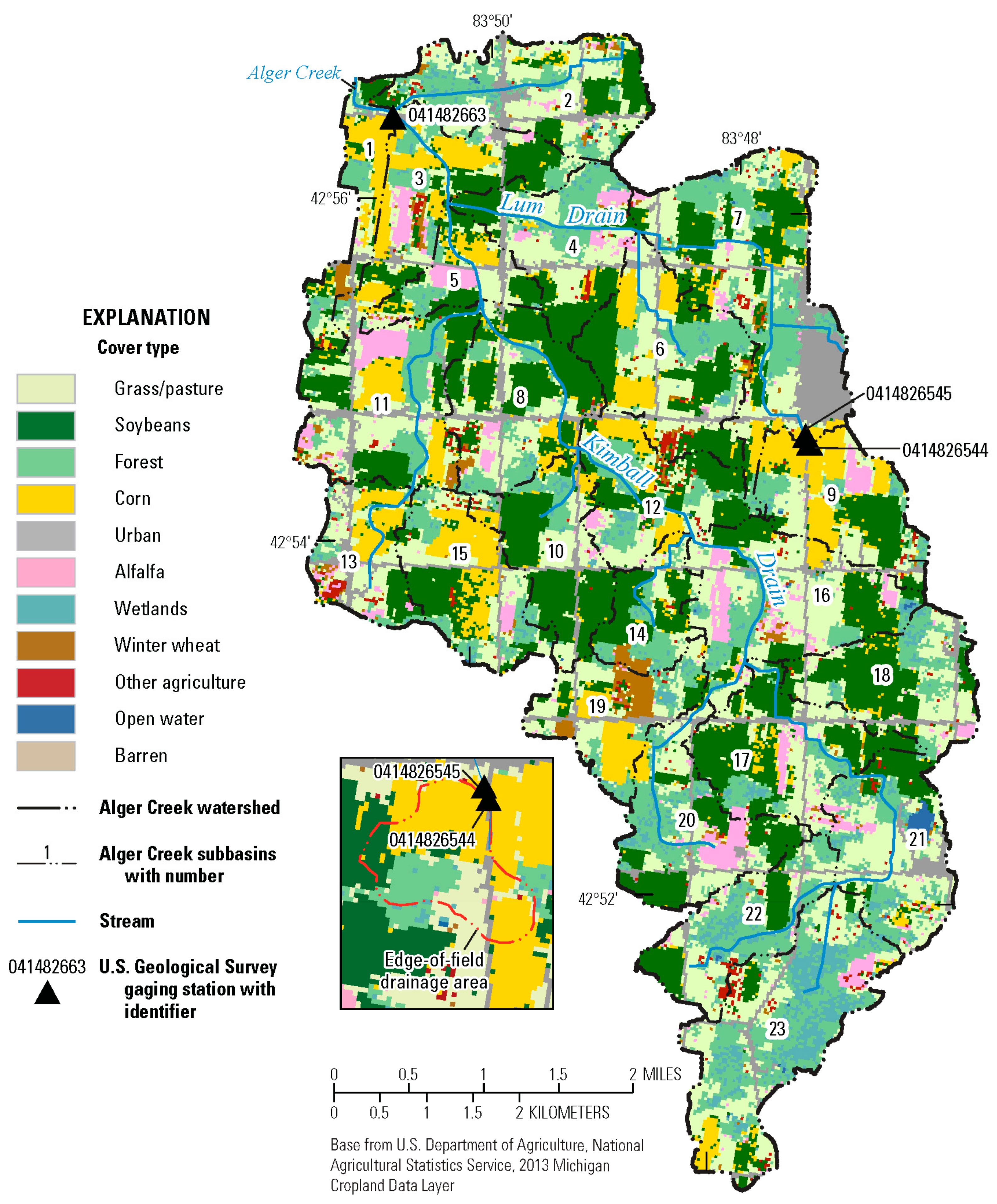
2.1. Study Watershed

The Saginaw River basin is located in the center of the Lower Peninsula of Michigan, and, at nearly 22,500 km² in size, is the State’s largest drainage basin. The Hydrologic Unit Code (HUC) 12 watershed that is the subject of this modeling study is Alger Creek, a tributary of the Saginaw River through the Flint River. It is approximately 50 km² and is located entirely within Genesee County, Michigan (Figure 1). The Alger Creek watershed consists of predominantly cultivated crop (primarily corn and soybean) and hay/pasture land cover, with pockets of woods (as mixed forest, deciduous forest, and woody wetland) and residential development (Figure 2) [24]. The Soil Survey Geographic Database (SSURGO) describes most soil in the basin as dominated by loam and silty loam [25]. The basin is mostly flat, with 41 m of relief and 1.3% slope within the entire basin [26]. The basin topography is highly conducive to flooding during heavy or long duration precipitation events. This basin has a temperate climate, and the average precipitation measured in the study area from 2012 to 2017 was 808 mm annually [27].

Alger Creek is located south of the city of Swartz Creek, MI (Figure 1), and is composed of two major tributaries: Kimball Drain and Lum Drain. Alger Creek is heavily influenced by agricultural activities as there is very little riparian area along its banks for most of its watershed. Both Kimball Drain and Lum Drain are maintained as county drains by the Genesee County Drain Commission, meaning that these drains can have their beds and banks reshaped to ensure free passage of water off of farmland and through their channels. Less than 0.7 km downstream from the USGS gauging station (USGS 041482663 Alger Creek at Hill Road near Swartz Creek, MI), Alger Creek joins with the West Branch Swartz Creek. The EOF study area in Michigan is located on a private field (Figure 2). The study field is a row crop parcel that rotates annually between corn and soybeans. There are two monitoring stations on the study field: one that evaluates and samples surface runoff (USGS 0414826544) and another that measures subsurface flow through a tile drain (USGS 0414826545). Tile maps were not available for the study field. Contributing areas were estimated using satellite imagery (for the tile site) and lidar (for the surface runoff site). Estimated contributing areas for the tile and surface runoff stations are 28.6 and 60.6 ha, respectively. As seen in Figure 2, runoff is from more than a single field—additional agricultural fields, forest, and pasture areas also are included in the drainage area delineation.

2.2. Data Collection and Processing

USGS collected extensive data at multiple gauges within the Alger Creek watershed, including the HUC 12 outlet, the EOF surface site, and the EOF tile site. Methods of data collection, sample processing, and data analysis at the EOF and tile sites follow procedures provided by Stuntebeck et al. [28]. Streamflow at the monitoring sites were recorded continuously during the study period. Water-quality samples were collected and analyzed for suspended sediment, chloride, nitrate plus nitrite, ammonium, unfiltered total Kjeldahl nitrogen (TKN), orthophosphosphate, and TP. Total nitrogen (TN), organic nitrogen, and particulate phosphorus (PP) were calculated. Terminology substitution for analytically-determined orthophosphate [29] as dissolved reactive phosphorus, or DRP [30], is used in this paper.

The Water and Environmental Analysis Laboratory at the University of Wisconsin in Stevens Point, Wisconsin analyzed all samples. Streamflow and water-quality sample concentrations were used to compute daily loads using the Graphical Constituent Loading Analysis System (GCLAS) [31]. Streamflow, sample results, and daily loads at the HUC 12 outlet are stored in the USGS National Water Information System [32]. The daily loads at the EOF and tile sites produced from GCLAS are available at USGS ScienceBase [33].

2.3. Soil and Water Assessment Tool Model Input and Setup

The USDA Agricultural Research Service developed the watershed-scale, process-based SWAT model [34,35,36,37]; it is currently the most widely used deterministic hydrological model in the world [35]. ArcSWAT 2012 was used to build the Alger Creek SWAT model [38]. This project used SWAT2012 Revision 665b, which was specifically modified to print the soluble or dissolved phosphorus in tile drainage to the HRU output. Input layers to model development were described in Merriman [39].

2.3.1. Watershed and Subbasin Delineation

Watershed delineation is the first step in the model setup, and begins by using a digital elevation model and hydrography dataset to define the flow path and partition the basin into subbasins. The National Elevation Dataset with a 10-m resolution [26] and the National Hydrography Dataset Plus [40] were used in this study. The subbasin delineation of the Alger Creek watershed resulted in 23 subbasins (Figure 2).

2.3.2. Hydrologic Response Units Development

After subbasin delineation, HRUs—where landscape processes are computed—are developed. By default in SWAT, HRUs within a subbasin with similar landuse, soil, and slope layers are lumped together [41]; however, this SWAT default lumping decreases the user’s ability to manipulate each field’s unique management characteristics [42]. A simple way to avoid this aggregation is to set HRU thresholds in the model to zero [21,43]. However, more detailed procedures presented by Daggupati et al. [21] and Kalcic et al. [20] allow each agricultural field to remain its own HRU, thereby the user can control each field’s management. Because this study looks at BMPs at the field scale, the Daggupati et al. [21] and Kalcic et al. [20] methodologies were loosely followed.

A Memorandum of Understanding was signed between USGS and USDA-NRCS to allow USGS access the National Conservation Planning (NCP) Database, which stores the repository of NRCS-funded BMPs throughout the United States. The spatially explicit NCP data allowed USGS to address the spatial complexity of BMPs throughout the small watershed. A field outline layer was developed using the Common Land Unit (CLU) data layer, which defines individual farm fields receiving USDA assistance. In the Alger Creek watershed, the CLU outlined 806 fields. The CLU does not cover the entire Alger Creek watershed; there are gaps in it for residential, urban, forested, and wetlands. Homesteads, urban areas, forests, and fields not receiving NRCS assistance were manually delineated. The National Wetlands Inventory from the U.S. Fish and Wildlife Service [44] was overlaid to incorporate 298 ha of wetlands and ponds. The SWAT input landuse layer was made using the majority value for each outlined field from the 2013 Cropland Data Layer (CDL) [24]. Most of the CDL layers are available at a 30-m resolution; however, the resolution of 2008 and 2009 CDL was 56 m, and these layers were resampled to a 30-m resolution for consistency. Altogether, there were 1134 fields encompassing the Alger Creek watershed. The outline created for landuse was also used for the soil layer definition, where the majority SSURGO soil type present in each field was used. A slope layer was created using “single slope option” in ArcSWAT, and HRU thresholds for landuse, soils, and slope were set to zero to keep the field boundaries as delineated. Most HRUs represented one farm field or contiguous landuse; however, when a field contained a topographic divide and drained to multiple subbasins, then that field was divided into separate HRUs. This occurred to numerous fields, increasing the final number of HRUs to 1544.

2.3.3. Weather

Three National Climatic Data Center (NCDC) [45] weather stations were selected for use in the Alger Creek model (Figure 1 and

Table 1. U.S. Geological Survey gauging stations and National Climatic Data Center weather stations in the Alger Creek watershed, Michigan.

Owner	Site ID	Station Name	Parameter	Period of Record Used
USGS	041482663	Alger Creek At Hill Road Near Swartz Creek, MI	Streamflow Water Quality	4/13/2012 to 9/30/2016
USGS	0414826544	Trib To Lum Drain Adj Sharp Rd Nr Swartz Creek, MI	Surface runoff Water Quality	4/13/2012 to 9/30/2016
USGS	0414826545	Trib To Lum Drain Near Swartz Creek, MI (Tile)	Tile flow Water Quality	4/17/2012 to 9/30/2016
NCDC	USW00014826	Flint Bishop International Airport MI US	Precipitation Temperature	1/1/1960 to 9/30/2016
NCDC	USC00204793	Linden WWTP MI US	Precipitation Temperature	1/1/2002 to 9/30/2016
NCDC	USC00202328	Durand WWTP MI US	Temperature	12/1/2003 to 9/30/2016
Notes: USGS = U.S. Geological Survey; NCDC = National Climatic Data Center.

). Each SWAT subbasin uses the closest station for daily precipitation and temperature data. For any days with missing record, the SWAT weather generator filled in those days using averages from a statistics table built from observations at the Flint Bishop International Airport. The weather generator was also used to calculate daily values for solar radiation, wind speed, and relative humidity.

2.3.4. Tile Drainage

Agricultural fields that were composed primarily of soils with hydrologic soil groups of C or D were assumed to be tile drained. This resulted in 432 HRUs or approximately 36% of the Alger Creek watershed being drained by subsurface tiles in the SWAT model.

2.3.5. Management

Based on the 2007–2014 CDLs, a suite of two-, three-, and five-year rotations were developed that most closely represented actual crops planted throughout the watershed during the calibration period (2012–2014). The following five basic crop rotations were developed: two-year Corn–Soy, three-year Corn–Soy–Soy, three-year Corn–Soy–Wheat, five-year Soy–Wheat–Soy–Corn–Soy, and five-year Alfalfa. These rotations were implemented in a staggered fashion to more realistically distribute the years when crops were present.

Details of agricultural management operations were developed in consultation with the local NRCS staff most familiar with common practices in the Alger Creek watershed. Operation information included dates of management activities and the types of agricultural machinery used as well as fertilizer application rates (

Table 2. Agricultural management operations used in the Alger Creek watershed SWAT model by crop.

		Date of Operation
Operation	Crop:	Corn	Soybeans	Winter Wheat		Alfalfa
	Year:	1	1	1	2	1	2-5
Kill Date						1 April
Secondary Tillage—Field cultivator		20 April	20 April			25 April
Planting		5 May	10 May	15 October		1 May
Fertilizer 1		1 May 1		12 October 1,4		2 May 6	2 June 6
Fertilizer 2		4 May 2			14 April 5
Fertilizer 3		5 June 3
Harvest 1 $		25 October	10 October		15 July	15 July	1 June
Harvest 2						1 September	15 July
Harvest 3							1 September
Primary Tillage—Chisel Plow		1 November	1 November *		1 November

Fertilizer application rates and fertilizer content in percent N-P-K: ¹ 112 kg ha⁻¹ 11-52-0. ² 65 kg ha⁻¹ 10-34-0. ³ 168 kg ha⁻¹ anhydrous ammonia. ⁴ 44.8 kg ha⁻¹ 46-0-0. ⁵ 196 kg ha⁻¹ 46-0-0. ⁶ 140 kg ha⁻¹ 11-52-0. ^$ For corn, soybeans, and winter wheat harvest, harvests are simulated by the harvest and kill operation (MGT_OPT = 5) in SWAT. Alfalfa harvests are harvest only which is a cutting that removes biomass but allows the plant to continue growing (MGT_OPT = 7). * If soybeans are followed by winter wheat in a crop rotation, then there is no fall tillage prior to planting winter wheat.

).

2.3.6. Best Management Practice Implementation

The NCP database identified 1208 instances of practices applied or planned within the Alger Creek watershed during the period 2005–2018. These instances are not equivalent to the number of unique BMPs, as a practice could appear in the database for several successive years and each appearance would be a distinct instance despite representing a single BMP implementation. Practices with five or fewer implementations were not modeled due to privacy concerns. Four additional practices that were not expected to result in nutrient reductions were also excluded from the analysis, after consultation with NRCS: forest wildlife structures, integrated pest management, upland wildlife habitat management, and use techniques to reduce pesticide drift. These exclusions reduced the number of BMP instances in the Alger Creek watershed to 796.

The overwhelming majority of BMPs (95% of fields with a BMP) modeled in the Alger Creek watershed were funded by GLRI. Structural BMPs were not common in this watershed; all of the funded BMPs were non-structural in nature and were modeled by adjusting management operations. According to the NCP database there were primarily four types of BMPs implemented in the Alger Creek watershed: cover crops (CC), nutrient management plan (NMP), reduced till (RT), and no-till (NT). The watershed had 216 BMPs either applied or planned on 108 fields.

BMPs were modeled similarly to techniques described in Arabi et al. [16]. The primary cover crop in the Alger Creek watershed is cereal rye. CC were implemented in the model by adjusting the management operation dates such that primary tillage occurred on 30 October and the cereal rye was planted on 1 November then killed on 1 April. The kill operation on 1 April of each year is accomplished through spraying the crops, and no soil disturbance is simulated. If a field was planted in winter wheat, then no cover crop was planted that winter. After the wheat was harvested the following summer, however, then the cover crop would be planted.

Two additional BMPs were simulated in the hypothetical scenarios discussed in the next section: conservation crop rotation (CCR) and filter strips (FS). CCR was implemented in the model by adding winter wheat into a corn–soybean rotation once every five years. When applied to individual fields, the year in which wheat was planted was staggered during Years 1–5 so that the percentage of fields in wheat was approximately equal each year. FS were implemented in the model using the Scheduled Management Operations (.ops) file by using the following default SWAT parameters: the ratio of field area to filter strip area was 40; the fraction of the HRU which drains to the most concentrated 10% of the filter strip area was 0.5; and the fraction of the flow which is fully channelized and not subject to filtering or infiltration effects was 0.

2.4. Scenarios

To help evaluate the effect of various conservation practice combinations on sediment and nutrient loadings, several scenarios were modeled. The first set of scenarios were designed to quantify the effect of GLRI and non-GLRI funded BMPs in the Alger Creek watershed. The number of BMPs modeled in each scenario is shown in

Table 3. BMP implementation scenarios investigated with the Alger Creek watershed SWAT model, Michigan.

Modeled Scenarios	Practices Added	Total Fields with BMPs (BMP Count)	Hectares of BMPs	Percent of Watershed with BMPs
Baseline	--	0 fields (0 BMPs)	0	0%
Applied GLRI BMPs	CC on 6 fields	52 fields (67 BMPs)	369	7.4%
	NMP on 15 fields
	NT on 40 fields
	RT on 6 fields
All Applied BMPs (GLRI + nonGLRI BMPs)	No non-GLRI funded Applied BMPs	52 fields (67 BMPs)	369	7.4%
All Applied + Planned GLRI BMPs	CC on 65 fields	103 fields (206 BMPs)	803	16.1%
	NMP on 74 fields
All Contracted BMPs (All Applied and Planned: GLRI + nonGLRI BMPs)		108 fields(216 BMPs)	815	16.4%
	CC on 5 fields
	NT on 5 fields
Low	CC on 14 fields	144 fields (325 BMPs)	1046	21.0%
	NMP on 9 fields
	NT on 21 fields
	RT on 28 fields
	CCR on 37 fields
Medium	CC on 104 fields	196 fields (620 BMPs)	1232	24.7%
	NMP on 98 fields
	NT on 128 fields
High	CC on 167 fields	363 fields (1145 BMPs)	2107	42.3%
	NMP on 167 fields
	NT on 167 fields
	FS on 23 fields

Notes: BMPs = best management practices; CC = cover crops; CCR = conservation crop rotation; FS = filter strip; GLRI = Great Lakes Restoration Initiative; NMP = nutrient management plan; NT = no-tillage; RT = reduced tillage.

. The role of non-GLRI funded BMPs in the Alger Creek watershed was minimal. According to the NCP database, only five fields implemented any BMPs that were not funded by GLRI. As scenarios progressed, more practices may be added to a field or an existing practice may be enhanced (i.e., from RT to NT), but once installed a practice was not removed. BMPs were in place during the entire simulation period; they were not implemented on specific calendar dates.

The total area of fields implementing different BMP combinations is summarized by scenario in Table 3 and

Table 4. Total area of BMP combinations by scenario investigated with the Alger Creek watershed SWAT model, Michigan. (Modeled scenarios: AA =All Applied BMPs; AA + PG = All Applied + Planned GLRI BMPs; AC = All Contracted BMPs; Low; Med = Medium; High).

BMP Combinations	Area (ha)
	AA	AA + PG	AC	Low	Med	High
CC	32	55	55	23
CCR				1
NMP		202	202	162	4	4
NT	204
RT	69	69	69	8
CC + NMP		209	209	121
CC + NT			12	67
CCR + NT				1
CCR + RT				175
NT + NMP	65
CCR + CC + NT				1
CCR + RT + NMP				39
CC + NT + NMP		268	268	348	914	1703
CC + NT + NMP + FS						87
CCR + CC + RT + NMP				88
CCR + CC + NT + NMP				12	314	261
CCR + CC + NT + NMP + FS						53
Total	369	803	815	1046	1232	2107

Notes: BMPs = best management practices; CC = cover crops; CCR = conservation crop rotation; FS = filter strips; GLRI = Great Lakes Restoration Initiative; NMP = nutrient management plan; NT = no-tillage; RT = reduced tillage.

. While NT was a common practice in the All Applied scenario, that was the only scenario which contained any fields with NT as a single practice. When Planned GLRI practices were added to the model, those NT fields had CC and NMP implemented as well, and that 204 ha are included in the CC + NT + NMP area of the All Applied and Planned GLRI (AA + PG) scenario. In the All Contracted scenario, there were 216 BMPs installed on 108 fields, encompassing 815 ha. While some of these fields (326 ha) implemented a single practice, the majority of fields with a BMP had two or more practices installed.

The second set of scenarios modeled were hypothetical levels of implementation that were intended to quantify what the effects of increased adoption of BMPs would be on sediment and nutrient loadings. These scenarios were developed in consultation with local NRCS to determine what practices would be of the most interest to local producers. The Low scenario targeted those fields which already contained a BMP in the Applied scenario but no additional BMPs in the Planned scenarios and upgraded them to implement the trio of CC + NT + NMP. The Low scenario also implemented practices in the NCP database that were designated “Certified Technical Assistance” (CTA), where no financial assistance was provided but the local NRCS agents provided technical guidance to the producer. The Medium scenario similarly upgraded any remaining field with 1 or 2 BMPs to the full trio of CC + NT + NMP. An additional 25% of remaining agricultural fields also had this trio of BMPs implemented. The High scenario implemented the trio of CC + NT + NMP on all remaining agricultural fields and installed a filter strip on one field in each of the 23 subbasins. The BMP coverage simulated with these Low, Medium, and High hypothetical levels of implementation correspond to approximately 40%, 60%, and 100%, respectively, of the agricultural fields in the HUC 12 watershed; this equates to 21%, 25%, and 42%, respectively, of the total land area in the Alger Creek watershed.

2.5. Calibration

The model was calibrated to the All Applied BMPs scenario, which incorporated BMPs that were certified as Applied in the NCP database, thus the calibration would best reflect the practices installed in the Alger Creek watershed during the calibration period (2012–2014). Streamflow, sediment, and nutrients were calibrated at the Alger Creek USGS gauging station (041482663), which gauges approximately 93% of the watershed. Simulated nitrate (NO₃-N) was calibrated to the observed summation of nitrate + nitrite. The model was calibrated at a monthly time step; daily data were also used to assist with calibration of timing parameters. In the Alger Creek watershed, the EOF data were not used for direct calibration of the model due to the uncertainty of the area drained by the monitored tile system. While the total flow and load leaving the tile are measured, the area contributing to this volume is estimated; therefore, it was not clear which HRUs and more likely which fraction of those HRUs to use for comparisons to observed data. The calibration was performed by simulating the SWAT model from 2007 to 2014 including a five-year warmup period as recommended by Daggupati et al. [46].

Calibration was completed using a combination of manual calibration and automated calibration using SUFI-2 in SWAT-CUP [47]. Tile drainage was implemented using the lag time method (ITDRN = 0). During initial simulations, the model was not producing tile flow in the winter months, yet the EOF monitoring site’s tile was flowing at times in winter months. In SWAT the daily soil temperatures are currently determined empirically as a function of several variables, including the previous day’s soil temperature at certain depth, the average annual air temperature, the current day’s soil-surface temperature, and downward position of the soil profile [41]. A lag coefficient is introduced that influences the previous day’s temperature and current day’s temperature. However, Bélanger [48] found that SWAT underestimates soil temperature during winter even with the adjusted lag factor, which reduces tile flow as tile flow is not simulated while soils are frozen. A physically-based soil-temperature module to address this situation would be an improvement in the SWAT model. To increase soil temperatures enough to allow tile flow while maintaining some of the daily climatic fluctuations, in this study, all negative air temperatures were replaced with one-tenth of their observed value.

After adjusting the daily minimum and maximum air temperatures, snow parameters were fit first using auto-calibration techniques. Final snow parameters were set and then hydrology parameters were calibrated using monthly streamflow data. Parameters related to sediment were investigated next, followed by parameters that primarily affected nitrogen and phosphorus processes. Calibration performance was evaluated using various statistics as well as visual comparison of simulated and observed daily streamflow values; both hydrographs and flow duration curves were used to evaluate model performance.

Quantitative statistics were used to evaluate the relationship between observed and simulated values as recommended in Moriasi et al. [49,50]. The quantitative statistics applied in this study are Nash–Sutcliffe simulation efficiency (NSE), the coefficient of determination (R²), and percentage bias (PBIAS). NSE is the most accepted and implemented statistical standard for the evaluation of performance in watershed modeling [35,46,51] and is well-known for estimating peaks of model responses. The NSE value ranges from 1 to −∞, where a value of 0.75–1 indicates a very good model fit, 0.65–0.75 is good, 0.50–0.65 is satisfactory, and <0.5 is unsatisfactory. Higher values of R² demonstrate a better fit of the simulated data to the observed data. On the other hand, PBIAS is used to assess the average tendency of system response. The optimal value of PBIAS is 0.0%, where absolute values of PBIAS <10%, <15%, and <25% indicate a very good model fit for streamflow, sediment, and nutrients, respectively, 10–15%, 15–30%, and 25–40% indicate good, 15–25%, 30–55%, and 40–70% indicate satisfactory, and >25%, >55%, and >70% indicate unsatisfactory. Positive values of PBIAS indicate model underestimating bias and negative values indicate model overestimating bias [52].

After calibration, the additional scenarios were prepared by using the calibrated model but adding the practices specified in Table 3, or, in the case of the baseline scenario, by removing all of the NCP database practices. This baseline scenario was developed to compare all other scenarios against.

3. Results and Discussion

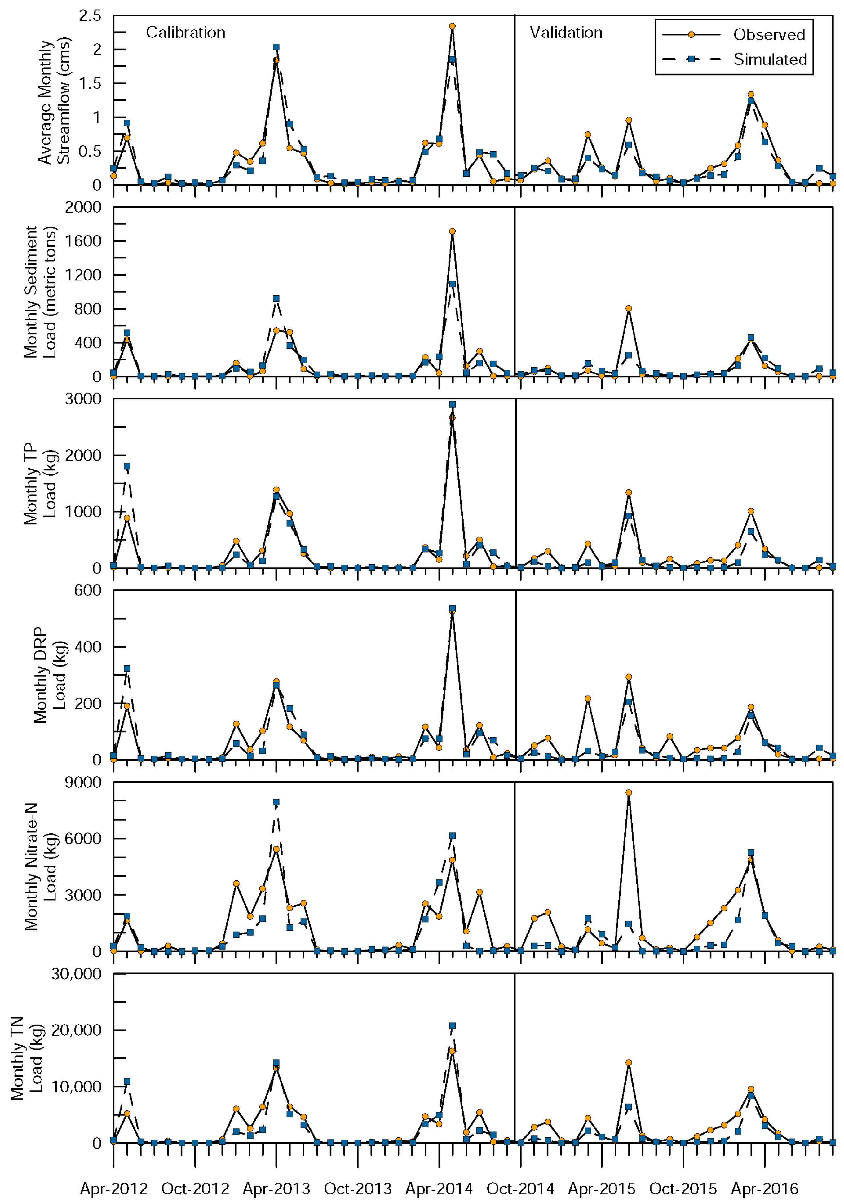
3.1. Calibration and Validation

Generally, the model did a good job of capturing streamflow volume on a monthly basis. However, low and medium streamflows were frequently overestimated, with the notable exception of January–March 2013 when SWAT undersimulated streamflow (Figure 3). Final calibration parameter values and method selections are presented in

Table 5. SWAT methods and parameters for the Alger Creek watershed model, Michigan.

Parameter Type	Parameter	File	Description	Default Value	Model Range	Calibrated
Snow	SMTMP	.bsn	Snowmelt base temperature (°C)	0.5	−5 to 5	4.9
Snow	SFTMP	.bsn	Snowfall temperature (°C)	1	−5 to 5	1.7
Snow	SMFMX	.bsn	Maximum snowmelt factor for June 21 (mm H2O/°C-day)	4.5	0 to 20	3.2
Snow	SMFMN	.bsn	Minimum snowmelt factor for December 21 (mm H2O/°C-day)	4.5	0 to 20	2.6
Snow	SNOCOVMX	.bsn	Minimum snow water content that corresponds to 100% snow cover (mm)	1	0 to 500	48
Hydrology	CN2	.mgt	Initial SCS runoff curve number for moisture condition II	Dependent on soils and landuse		−19.80%
Hydrology	ESCO	.hru	Soil Evaporation compensation factor	0.95	0 to 1	0.95
Hydrology	REVAPMN	.gw	Threshold depth of water in the shallow aquifer required for “revap” or percolation to the deep aquifer to occur (mm)	750	0 to 1000	500
Hydrology	GWQMN	.gw	Threshold depth of water in the shallow aquifer required for return flow to occur (mm)	1000	0 to 5000	Default
Hydrology	GW_REVAP	.gw	Groundwater “revap” coefficient	0.02	0.2 to 0.20	0.066
Hydrology	GW_DELAY	.gw	Groundwater delay (days)	31	0 to 2000	14
Hydrology	ALPHA_BF	.gw	Base flow recession constant	0.048	0 to 1	Default
Hydrology	CH_N2	.rte	Manning’s coefficient for channel	0.014	0 to 0.3	0.075
Tile Drainage	ITDRN	.bsn	Tile drainage method; 0 = lag time method; 1 = Hooghoudt and Kirkham tile drain equations	0	0 or 1	0
Tile Drainage	DEP_IMP	.hru	Depth to impervious layer in soil profile in tile drained fields (mm)	6000	0 to 100,000	1200
Tile Drainage	DEP_IMP	.hru	Depth to impervious layer in soil profile in undrained fields (mm)	6000	0 to 100,000	3500
Tile Drainage	Ddrain	.mgt	Depth to drains (mm); must be >0 to initiate tile drainage	0	0 to 2000	1000
Tile Drainage	Tdrain	.mgt	Time to drain soil to field capacity (hours)	0	0 to 72	48
Tile Drainage	Gdrain	.mgt	Drain tile lag time (hours)	0	0 to 100	24
Sediment	SPCON	.bsn	Linear parameter for calculating the maximum amount of sediment that can be reentrained during channel sediment routing	0.0001	0.0001 to 0.01	0.0008
Sediment	SPEXP	.bsn	Exponent parameter for calculating sediment reentrained in channel sediment routing	1	1.0 to 2.0	1.4
Sediment	PRF_BSN	.bsn	Peak rate adjustment factor for sediment routing in the main channel	1	0.5 to 2.0	1.8
Sediment	ADJ_PKR	.bsn	Peak rate adjustment factor for sediment routing in tributary channels	1	0.5 to 2.0	0.5
Phosphorus	PSP	.bsn	Phosphorus availability index	0.4	0.01 to 1	0.37
Phosphorus	PPERCO	.bsn	Phosphorus percolation coefficient (10 m3 Mg−1)	10	10.0 to 17.5	15.2
Phosphorus	PHOSKD	.bsn	Phosphorus soil partitioning coefficient (m3 Mg−1)	175	100 to 200	188
Phosphorus	P_UPDIS	.bsn	Phosphorus uptake distribution parameter	20	0 to 100	98.3
Phosphorus	SOL_CRK	.sol	Maximum crack volume of soil profile (fraction)	0.5	0 to 1	0.25
Phosphorus	SOL_P_MODEL	.bsn	Soil Phosphorus Model (0 = original; 1 = new soil P model)	0	0 or 1	1
Nitrogen	NPERCO	.bsn	Nitrate percolation coefficient	0.2	0 to 1	0.161
Nitrogen	CDN	.bsn	Denitrification exponential rate coefficient	1.4	0.0 to 3.0	0.317
Nitrogen	SDNCO	.bsn	Denitrification threshold water content	1.1	0 to 1	0.991
Nitrogen	N_UPDIS	.bsn	Nitrogen uptake distribution parameter	20	0 to 100	32.4
Nitrogen	ANION_EXCL	.sol	Fraction of porosity (void space) from which anions are excluded	0.5	0 to 1	0.2

. Water balance components as a percentage of total water yield during the calibration period were 49% surface runoff, 28% tile flow, 15% ground water, and 8% lateral flow. Monthly plots of simulated and observed streamflow, sediment, TP, DRP, nitrate, and TN are shown in Figure 3.

Calibrating the model based on limited observed data (less than three years) did not allow for a wide variation in the climate. While the calibration period contained natural variability in precipitation and streamflow, the range was limited. There were no extended dry periods or extended wet periods, and this may have caused model bias. This may explain the poorer performance during the validation period which contained the driest year (2015) of the five-year calibration and validation period. The validation period also contained multiple fall/winter storm events (November–December 2014 and November 2015–January 2016). This type of cold-weather runoff event was not present during the fall/winter months of the calibration period, and the model performed poorly during these months typically undersimulating streamflow and nutrient loading.

Calibration results are generally very good, whereas validation results are satisfactory (

Table 6. Calibration and validation monthly summary statistics for the Alger Creek watershed SWAT model, Michigan.

Constituent	NSE	PBIAS	R2	NSE	PBIAS	R2
	Calibration WY2012*-WY2014			Validation WY2015-WY2016
Flow	0.90	−6.7	0.91	0.83	17.6	0.88
Sediment	0.79	−1.1	0.81	0.54	3.5	0.57
TP	0.87	−7.1	0.91	0.73	41.8	0.87
DRP	0.88	−3.3	0.90	0.53	42.2	0.64
NO3-N	0.51	18.8	0.67	0.28	49.7	0.39
TN	0.77	6.7	0.84	0.60	48.2	0.80

* WY 2012 partial record. Notes: NSE = Nash–Sutcliffe simulation efficiency; PBIAS = percentage bias; R² = coefficient of determination; DRP = dissolved reactive phosphorus; NO₃-N = nitrate; TP = total phosphorus; TN = total nitrogen; WY = water year, the 12-month period 1 October–30 September designated by the calendar year in which it ends.

). Monthly NSE statistics ranged from 0.51 to 0.90, indicating calibration was satisfactory for NO₃-N and very good for flow, sediment, TP, DRP, and TN. Monthly PBIAS values were all very good and ranged from −7.1% to 18.8%. Monthly R² values for flow, sediment, TP, DRP, and TN were all between 0.81 and 0.91, whereas the monthly R² value for NO₃-N calibration was 0.67. During the two-year validation period, PBIAS statistics ranged from satisfactory (flow, TP, DRP, NO₃-N, and TN) to very good (sediment), and NSE statistics were unsatisfactory (NO₃-N), satisfactory (sediment, DRP, and TN), good (TP), and very good (flow).

Simulated and observed crop yields were compared after final calibration, and the model predicted higher corn and wheat yields and lower soybean yields than observed (

Table 7. Observed and simulated crop yields for the Alger Creek watershed SWAT model, Michigan.

	Average Annual Crop Yield (Metric Tons ha−1)		PBIAS
	Observed	Simulated	(%)
Corn	8.77	9.49	−8
Soybean	2.70	2.37	12
Winter Wheat	4.32	5.63	−30

Notes: PBIAS = percentage bias.

). The observed crop yields are from the Genesee County, MI crop yields as reported by USDA [53]. During 2012–2014, the observed average corn, soybean, and wheat yields were 8.8 metric tons per hectare (t ha⁻¹), 2.7 t ha⁻¹, and 4.3 t ha⁻¹, respectively. The simulated crop yields during that same three-year period were 9.5 t ha⁻¹, 2.4 t ha⁻¹, and 5.6 t ha⁻¹.

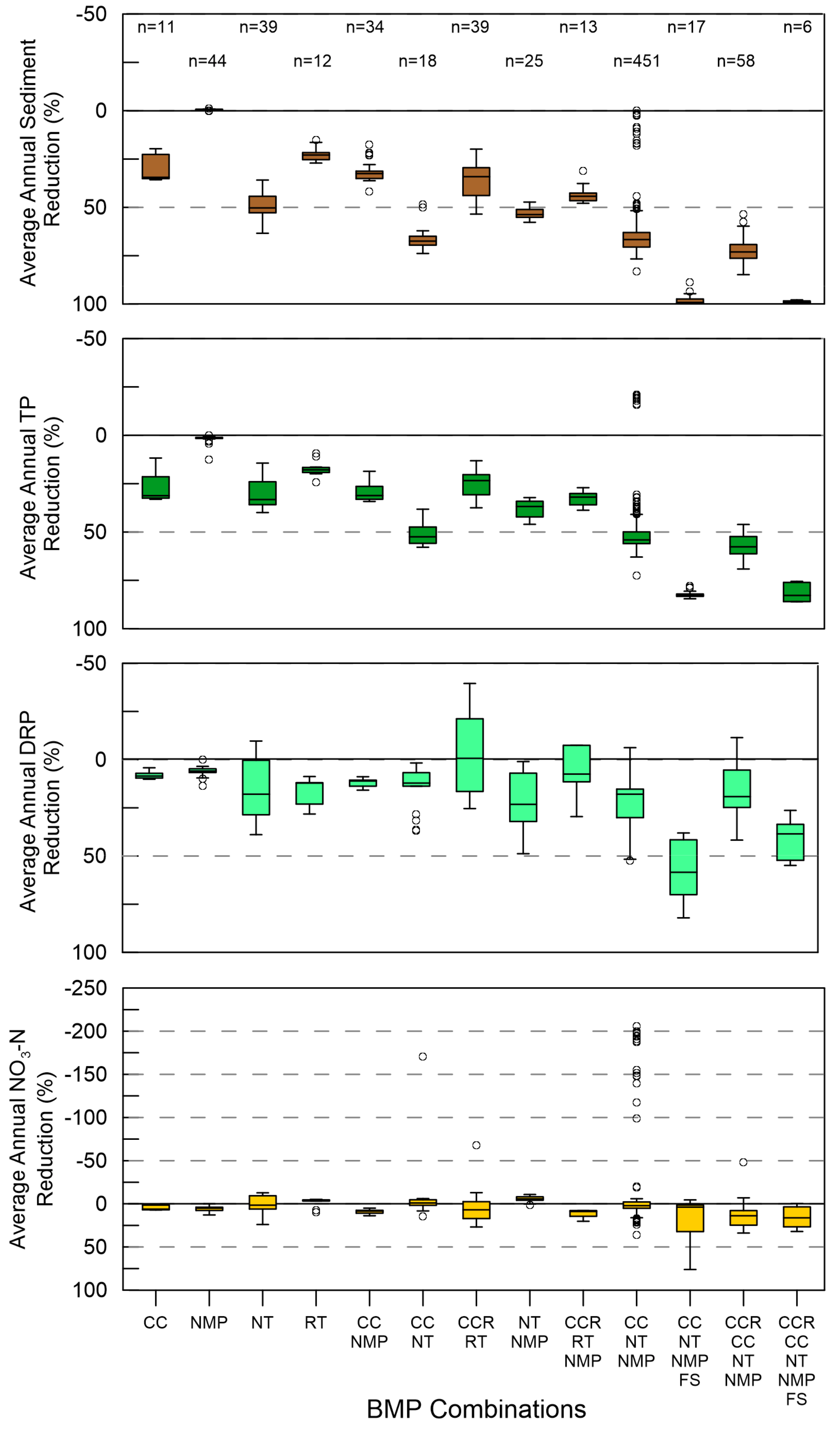
3.2. Effect of Best Management Practices at the Field-Scale

The effects of BMPs were evaluated by compiling annual sediment, TP, DRP, and NO₃-N losses for those HRUs containing BMPs for a 10-year simulation period (2005–2014). The differences in average annual losses were then aggregated by BMP combination. The percent reduction in sediment and nutrient losses were computed by subtracting the scenario of interest losses from the baseline scenario losses and then dividing by the baseline scenario losses.

Average annual reductions are presented in Figure 4 for each unique BMP or BMP combination that was implemented on more than five fields, independent of scenario. Due to the unique soil and land-use characteristics of individual HRUs as well as various crop rotations and spatial differences in precipitation, there was a lot of variability in the field-scale losses for each BMP combination. All constituents show a similar trend in that the average annual reductions in sediment and nutrient losses tend to be larger for fields with multiple BMPs implemented in combination than for fields with only a single BMP. The median average annual reduction by BMP combination is also summarized in

Table 8. Median average annual reductions in sediment and nutrient loadings by Best Management Practice (BMP) or BMP combination with the Alger Creek watershed SWAT model, Michigan. Negative values indicate an increase in sediment or nutrients.

BMP/BMP Combination	n	Median Average Annual Reductions (%)
		Sediment	TP	DRP	NO3-N
CC	11	34	31	8	6
NMP	44	−1	1	6	5
NT	39	50	33	18	2
RT	12	23	18	12	−4
CC + NMP	34	33	31	11	8
CC + NT	18	68	53	12	−1
CCR + RT	39	34	23	−1	7
NT + NMP	25	54	37	23	−6
CCR + RT + NMP	13	44	32	8	9
CC + NT + NMP	451	67	54	18	2
CC + NT + NMP + FS	17	99	83	58	4
CCR + CC + NT + NMP	58	73	58	19	14
CCR + CC + NT + NMP + FS	6	99	83	39	16

Notes: BMP = best management practice; CC = cover crops; CCR = conservation crop rotation; DRP = dissolved reactive phosphorus; FS = filter strips; GLRI = Great Lakes Restoration Initiative; n = number of HRUs with BMP/BMP combination implemented; NMP = nutrient management plan; NO₃-N = nitrate-nitrogen; NT = no-tillage; RT = reduced tillage; TP = total phosphorus.

.

Implementation of NMP as a single practice resulted in an almost imperceptible increase (median of −1%) in average annual sediment losses on most HRUs, and CC + NT + NMP, while reducing TP on more than 97% of the HRUs that implemented that combination, did cause an increase in average annual TP losses on 13 HRUs. All other practices resulted in average annual reductions in sediment and TP losses. The effectiveness of BMPs at reducing nutrient losses were much lower for the dissolved constituents (DRP and NO₃-N). Any BMP combination that included one of the tillage BMPs (NT or RT) saw an average annual increase of DRP or NO₃-N on at least one HRU. The adoption of these tillage BMPs occasionally created an increase in NO₃-N and DRP losses, as their implementation decreases surface runoff and increases infiltration. With higher soil moisture, there was more water contributing to tiles; this increase in tile flow can also create an increase in NO₃-N and DRP being leached through the soil profile.

When evaluating the modeled BMPs from the NCP database, the most commonly funded BMP was NMP, followed by CC. At the field-scale, the most effective single practice at reducing sediment, TP, and DRP was NT followed by CC, while the most effective single practice at reducing NO₃-N was CC. NMP was the least effective practice at reducing sediment and phosphorus loads but was comparable to other practices at reducing nitrate losses. The BMP combinations showing the greatest reductions in sediment and phosphorus losses were those that included FS. The addition of FS to a BMP combination at 23 common sites increased the median average annual reductions from 63% to 99% for sediment, from 52% to 83% for TP, from 18% to 52% for DRP, and minimally from 3% to 4% for NO₃-N.

In the All Contracted scenario (data not shown), which evaluated the performance of three single BMPs (CC, NMP, and RT) and three BMP combinations, median average annual reductions at the HRU level for sediment, TP, DRP, and NO₃-N were 35%, 32%, 12%, and 5%, respectively. When evaluating the hypothetical High scenario, the median average annual reductions at the HRU level (for those HRUs with BMPs) for sediment, TP, DRP, and NO₃-N were 68%, 54%, 18%, and 3%, respectively. These larger reductions in sediment and phosphorus losses reflect the effect of implementing BMP combinations rather than single BMPs, as the High scenario was almost exclusively HRUs with three or more BMPs implemented.

3.3. Effect of Best Management Practices at the Watershed-Scale

Field-scale reductions do not translate directly to reductions at the watershed outlet. When analyzing the effect of funded BMPs on sediment and nutrient losses leaving the watershed, the spatial extent of the BMPs is important. The fields with BMPs implemented range from 7% of the watershed in the Applied GLRI/All Applied scenario to 16% in the AA + PG and All Contracted scenarios. With less than 10% of the watershed implementing BMPs in the All Applied scenario, the reductions of 3% or less for sediment, TP, and DRP and an increase of less than 1% in NO₃-N losses were modest (Figure 5). Surface runoff, sediment and phosphorus loads by scenario and subbasin are mapped in Figure 6; only eight subbasins (1, 3, 5, 11, 14, 18, 19, and 20) show any perceptible reductions in the All Applied scenario for one or more constituent. Average annual sediment, TP, DRP, and NO₃-N reductions at the watershed outlet in the AA + PG scenario were 1%, 7%, 5%, and 2%, respectively. This scenario represents the effect of all GLRI funded practices. Additional reductions are visible at the subbasin level for subbasins 4, 16, and 17. Only 12 ha of non-GLRI funded BMPs were modeled in the watershed as part of the All Contracted scenario. These BMPs in comparison contributed minimally to the sediment and nutrient load reductions at the watershed outlet, as the average annual sediment, TP, DRP, and NO₃-N reductions in the All Contracted scenario were nearly unchanged at 0.5%, 7%, 5%, and 1%, respectively (Figure 5).

In the hypothetical Low, Medium, and High scenarios, the percentage of the Alger Creek watershed with implemented BMPs was 21%, 25%, and 42% respectively. At these levels of implementation, the effects were far more pronounced. The Low scenario represented the most diverse mixture of BMPs with more than 13 different BMP combinations modeled. Of all the hypothetical scenarios, this scenario actually produced the greatest reduction (4%) in nitrate at the watershed outlet. As the Medium and High scenarios implemented more NT practices, more fields saw an increase in their NO₃-N losses; with the universal implementation of NT in the High scenario, this increase was seen at the watershed outlet as well.

Average annual sediment, TP, DRP, and NO₃-N reductions at the HUC 12 outlet were 1%, 11%, 7%, and 4%, respectively, in the Low scenario; 3%, 18%, 11%, and 0.5%, respectively, in the Medium scenario; and 12%, 31%, 21%, and −4%, respectively, in the High scenario. In the High scenario, nearly 60% of the watershed was non-agricultural and implemented no BMPs, which subsequently saw no reductions at the field-scale in the various scenarios. It is important to understand the role of various landuses on the sediment and nutrient reductions in the watershed. Average annual yields are presented by landuse in

Table 9. Average annual field-scale yields by landuse in the All Applied scenario investigated with the Alger Creek watershed SWAT model, Michigan.

Landuse	Hectares	Sediment Yield (t ha−1)	TP Yield (kg ha−1)	DRP Yield (kg ha−1)	NO3-N Yield (kg ha−1)	TN Yield (kg ha−1)
Row crops	2103	0.83	0.96	0.10	6.80	11.72
Alfalfa	122	0.06	0.19	0.11	0.25	0.57
Pasture	1298	1.38	1.17	0.06	0.11	6.51
Urban	366	0.11	0.34	0.24	2.87	3.09
Forest	887	0.02	0.02	0.01	0.03	0.11
Water/Wetlands	209	0.01	0.02	<0.01	0.01	0.06

Notes: Row crops include fields with any combination of corn, soybeans, winter wheat and/or cereal rye. DRP = dissolved reactive phosphorus; NO₃-N = nitrate; TP = total phosphorus; TN = total nitrogen.

for the All Applied scenario, which is the most representative of current NCP BMP implementation. The row crops land-use category includes fields with cultivated crops in any combination of corn, soy, winter wheat, and possibly a cover crop of cereal rye. Alfalfa is only planted once every five years and is harvested 2–3 times per year. Pasture is not actively managed and is often located on fields with steeper slopes. On average, pasture lands had the highest sediment and TP losses followed by row crops. The highest NO₃-N losses were seen on row-cropped land followed by urban areas. These small areas of mostly residential developments had the highest DRP yields in the watershed.

The relative contributions of the different landuses were calculated by summing the field-scale losses by subbasin and across the watershed. This approach does not take into account reach-scale processes that may further increase or decrease the in-stream loads, but is instead a measure of the percent contribution to the reaches. The percent contributions by landuse for both the All Applied and High scenarios are presented in

Table 10. Load contribution by landuse in the All Applied and High scenarios investigated with the Alger Creek watershed SWAT model, Michigan.

	All Applied Scenario					High Scenario
Landuse	Sediment	TP	DRP	NO3-N	TN	Sediment	TP	DRP	NO3-N	TN
	(% of Total)					(% of Total)
Row crops	48.5	54.5	51.6	92.0	71.7	25.2	37.4	45.3	92.1	66.6
Alfalfa	0.2	0.6	3.5	0.2	0.2	0.3	0.9	4.0	0.2	0.2
Pasture	49.8	40.9	19.2	0.9	24.5	72.3	56.4	21.7	0.9	28.9
Urban	1.1	3.3	22.8	6.8	3.3	1.6	4.5	25.8	6.6	3.9
Forest	0.4	0.6	2.6	0.2	0.3	0.5	0.8	2.9	0.2	0.3
Water/Wetlands	0.1	0.1	0.2	0.0	0.0	0.1	0.1	0.3	0.0	0.0

Notes: Row crops include fields with any combination of Corn, Soy, Winter Wheat and/or Cereal Rye. DRP = dissolved reactive phosphorus; NO₃-N = nitrate; TP = total phosphorus; TN = total nitrogen.

. The BMP combinations implemented throughout this study were only placed on managed agricultural lands. The yields from the other landuses did not change throughout the scenarios, and as a result their relative contributions to the total load increased as the contribution from agricultural lands decreased. When looking at the DRP losses by subbasin (Figure 6), subbasins 4 and 7 do not see substantial reductions as the scenarios progress because most of their DRP is not sourced from agricultural land as urban/developed lands comprise more than 25% of these subbasins.

3.4. Model Limitations

Modeling each farm’s exact operational history is unfeasible, as the operational history of each individual farm is not known. The standard management operations used in this study are the best representation of average practices in the watershed. Only the BMPs present in the NCP database were modeled, even though the authors recognize that many other practices are present in the basin. BMPs could be farmer-initiated or state, county, locally, or otherwise funded and not be recorded in the NCP. Selzer et al. [54] reports that BMPs across the Saginaw Bay watershed are funded by local conservation districts, Michigan Department of Agriculture and Rural Development, and non-governmental organizations, and additionally the Michigan Agriculture Environmental Assurance Program provides technical assistance to farmers who want to install BMPs.

Agricultural management decisions are complex and based on multiple factors including weather, crop prices, previous crops grown, farming equipment available, etc. that vary annually. Therefore, management assumptions were made based on input from local NRCS agents and the NCP database BMPs. In addition, BMPs were not applied temporally to match NCP certified dates and management and maintenance of BMPs were assumed as constant over the simulation period.

Due to the lack of long-term monitoring data available within the Alger Creek watershed, the calibration period was less than three years, and a two-year period was used for validation. While not possible in this study, incorporating additional years of data would be beneficial to ensure the model was calibrated in a robust manner that included more climatic variability.

4. Conclusions

In this study, a SWAT model was developed for the Alger Creek watershed, Michigan to assess the effectiveness of USDA-RCS funded BMPs to reduce nutrients and to quantify nutrient reductions due to GLRI or other funding programs. Monthly calibration was performed at a single site near the watershed outlet and produced NSE and PBIAS statistics ranging from satisfactory (NO₃-N) to very good (flow, sediment, TP, DRP, and TN). During the two-year validation period, PBIAS statistics ranged from satisfactory (flow, TP, DRP, NO₃-N, and TN) to very good (sediment), and NSE statistics were unsatisfactory (NO₃-N), satisfactory (sediment, DRP, TN), good (TP), and very good (flow).

The calibrated model indicated that fields in row crop agriculture and pasture lands had the highest potential for sediment and TP losses; residential areas produced the highest DRP losses on a per hectare basis. The NCP database did not contain any BMPs on pasture lands or urban areas; therefore, this study does not evaluate BMP performance on various landuse types, only agricultural lands. The effects of agricultural BMPs on sediment and nutrient losses were evaluated by comparing various levels of BMP implementation during a 10-year simulation period. The effects were quantified as field-scale losses and as load reductions at the watershed outlet. In the Alger Creek watershed, GLRI funded the following BMPs and BMP combinations: CC, NMP, NT, RT, CC + NMP, and CC + NT + NMP. At the field-scale, NT was the most effective single practice to reduce sediment (median 50%), TP (median 33%), and DRP (median 18%), while CC was the most effective single practice to reduce NO₃-N (median 6%). BMP effectiveness varied greatly by field due to the unique combinations of soils, landuse, crop rotations, and precipitation patterns across the watershed. Some fields saw increases in DRP and NO₃-N losses with the adoption of NT or RT due to increased infiltration and soluble nutrient losses through tile drainage. BMP combinations of two or more practices produced greater sediment and nutrient reductions than single practices. CCR + CC + NT + NMP was the most effective non-structural BMP combination to reduce sediment (median 73%), TP (median 58%), DRP (median 19%), and NO₃-N (median 14%). The addition of FS to BMP combinations further increased sediment and nutrient reductions.

According to model simulations, GLRI practices on 803 ha (16.1% of the watershed) accounted for average annual sediment, TP, DRP, and NO₃-N reductions of 1%, 7%, 5%, and 2%, respectively, at the watershed outlet. The NCP database contained only five fields with BMPs funded by non-GLRI programs; with the addition of these BMPs, the average annual sediment, TP, DRP, and NO₃-N reductions at the watershed outlet were nearly unchanged at 0.5%, 7%, 5%, and 1%, respectively.

Hypothetical scenarios were used to evaluate sediment and nutrient losses under various levels of BMP implementation. In the hypothetical High scenario, a suite of BMPs (CC + NT + NMP) were implemented on all row crop fields (2107 ha), and FS were also installed on 23 fields; this resulted in overall average annual reductions in sediment, TP, DRP, and NO₃-N at the watershed outlet of 12%, 31%, 21%, and −4%, respectively. To achieve this level of implementation would require more than quadruple the number of BMPs currently funded by GLRI and other programs. Despite less than 50% of the Alger Creek watershed in row crop agriculture, this hypothetical scenario indicates that the implementation of non-structural agricultural BMPs can have a sizable effect on reducing sediment and phosphorus loads in the watershed.

References

1. Stow, C.A.; Dyble, J.; Kashian, D.R.; Johengen, T.H.; Winslow, K.P.; Peacor, S.D.; Francoeur, S.N.; Burtner, A.M.; Palladino, D.; Morehead, N.; et al. Phosphorus targets and eutrophication objectives in Saginaw Bay: A 35 year assessment. J. Great Lakes Res. 2014, 40, 4–10. [Google Scholar] [CrossRef]
2. Robertson, D.M.; Saad, D.A. Nutrient Inputs to the Laurentian Great Lakes by Source and Watershed Estimated Using SPARROW Watershed Models1. JAWRA J. Am. Water Resour. Assoc. 2011, 47, 1011–1033. [Google Scholar] [CrossRef] [PubMed]
3. Freedman, P.L. Saginaw Bay: An Evaluation of Existing and Historical Conditions; Environmental Protection Agency: Washington, DC, USA, 1974. [Google Scholar]
4. He, C.; Zhang, L.; DeMarchi, C.; Croley, T.E. Estimating point and non-point source nutrient loads in the Saginaw Bay watersheds. J. Great Lakes Res. 2014, 40, 11–17. [Google Scholar] [CrossRef]
5. International Joint Commission (IJC). Great Lakes Water Quality Agreement: Annex 4—Nutrients. Available online: http://www.ijc.org/en_/Great_Lakes_Water_Quality (accessed on 11 November 2017).
6. De Pinto, J.V.; Young, T.C.; McIlroy, L.M.; Meilroy, L.M. Great lakes water quality improvement. Environ. Sci. Technol. 1986, 20, 752–759. [Google Scholar] [CrossRef] [PubMed]
7. Dolan, D.M.; Chapra, S.C. Great Lakes total phosphorus revisited: 1. Loading analysis and update (1994–2008). J. Great Lakes Res. 2012, 38, 730–740. [Google Scholar] [CrossRef]
8. Komiskey, M.J.; Bruce, J.L.; Velkoverh, J.L.; Merriman-Hoehne, K.R. Great Lakes Restoration Initiative: Edge-of-Field Monitoring. Available online: http://wim.usgs.gov/geonarrative/glri-eof/ (accessed on 10 May 2017).
9. Merriman, K.R.; Gitau, M.W.; Chaubey, I. A Tool for Estimating Best Management Practice Effectiveness in Arkansas. Appl. Eng. Agric. 2009, 25, 199–213. [Google Scholar] [CrossRef]
10. Her, Y.; Frankenberger, J.; Chaubey, I.; Srinivasan, R. Threshold Effects in HRU Definition of the Soil and Water Assessment Tool. Trans. ASABE 2015, 58, 367–378. [Google Scholar] [CrossRef]
11. Baird & Associates. Sediment Trap Assessment Saginaw River, Michigan; Baird & Associates Technical Report; Baird & Associates: Madison, WI, USA, 2001. [Google Scholar]
12. Baird & Associates. Sediment Transport Modeling: Saginaw Bay, Saginaw River Basin; Baird & Associates Technical Report; Baird & Associates: Madison, WI, USA, 2000. [Google Scholar]
13. He, C.; DeMarchi, C.; Tao, W.; Johengen, T.H. Modeling Distribution of Point and Nonpoint Sources Pollution Loadings in the Saginaw Bay Watersheds, Michigan. In Geospatial Tools for Urban Water Resources; Lawrence, P.L., Ed.; Springer: Dordrecht, The Netherlands, 2013; pp. 97–113. ISBN 978-94-007-4734-0. [Google Scholar]
14. Giri, S.; Nejadhashemi, A.P.; Woznicki, S.A. Evaluation of targeting methods for implementation of best management practices in the Saginaw River Watershed. J. Environ. Manag. 2012, 103, 24–40. [Google Scholar] [CrossRef] [PubMed]
15. Baffaut, C.; Dabney, S.M.; Smolen, M.D.; Youssef, M.A.; Bonta, J.V.; Chu, M.L.; Guzman, J.A.; Shedekar, V.S.; Jha, M.K.; Arnold, J.G. Hydrologic and Water Quality Modeling: Spatial and Temporal Considerations. Trans. ASABE 2015, 58, 1661–1680. [Google Scholar] [CrossRef]
16. Arabi, M.; Frankenberger, J.R.; Engel, B.A.; Arnold, J.G. Representation of agricultural conservation practices with SWAT. Hydrol. Process. 2008, 22, 3042–3055. [Google Scholar] [CrossRef]
17. Gitau, M.W.; Gburek, W.J.; Bishop, P.L. Use of the SWAT model to quantify water quality effects of agricultural BMPs at the farmscale- level. Trans. ASABE 2008, 51, 1925–1936. [Google Scholar] [CrossRef]
18. Bosch, N.S.; Allan, J.D.; Selegean, J.P.; Scavia, D. Scenario-testing of agricultural best management practices in Lake Erie watersheds. J. Great Lakes Res. 2013, 39, 429–436. [Google Scholar] [CrossRef]
19. Legge, J.T.; Doran, P.J.; Herbert, M.E.; Asher, J.; O’Neil, G.; Mysorekar, S.; Sowa, S.; Hall, K.R. From model outputs to conservation action: Prioritizing locations for implementing agricultural best management practices in a Midwestern watershed. J. Soil Water Conserv. 2013, 68, 22–33. [Google Scholar] [CrossRef]
20. Kalcic, M.M.; Chaubey, I.; Frankenberger, J.R. Defining Soil and Water Assessment Tool (SWAT) hydrologic response units (HRUs) by field boundaries. Int. J. Agric. Biol. Eng. 2015, 8, 69–80. [Google Scholar]
21. Daggupati, P.; Douglas-Mankin, K.R.; Sheshukov, A.Y.; Barnes, P.L.; Devlin, D.L. Field-Level Targeting Using SWAT: Mapping Output from HRUs to Fields and Assessing Limitations of GIS Input Data. Trans. ASABE 2011, 54, 501–514. [Google Scholar] [CrossRef]
22. Runkel, R.L.; Crawford, C.G.; Cohn, T.A. Load Estimator (LOADEST): A FORTRAN Program for Estimating Constituent Loads in Streams and Rivers. In U.S. Geological Survey Techniques and Methods Book 4, Chapter A5; USGS: Reston, VA, USA, 2004; p. 69. [Google Scholar]
23. Komiskey, M.J.; Stuntebeck, T.D.; Frame, D.R.; Madison, F.W. Nutrients and sediment in frozen-ground runoff from no-till fields receiving liquid-dairy and solid-beef manures. J. Soil Water Conserv. 2011, 66, 303–312. [Google Scholar] [CrossRef]
24. USDA National Agricultural Statistics Service (NASS); Cropland Data Layer (CDL). 2013. Available online: https://nassgeodata.gmu.edu/CropScape/ (accessed on 30 May 2014).
25. Soil Survey Staff, Natural Resources Conservation Service, U.S.D. of A. Soil Survey Geographic (SSURGO) Database. Available online: https://sdmdataaccess.sc.egov.usda.gov (accessed on 17 January 2014).
26. U.S. Geological Survey National Elevation Dataset (NED). 1/3 Arc-Second. Available online: https://nationalmap.gov/elevation.html (accessed on 16 January 2014).
27. USGS. U.S. Geological Survey National Water Information System Data Available on the World Wide Web (USGS Water Data for the Nation); USGS: Reston, VA, USA, 2017.
28. Stuntebeck, T.D.; Komiskey, M.J.; Owens, D.W.; Hall, D.W. Methods of Data Collection, Sample Processing, and Data Analysis for Edge-of-Field, Streamgaging, Subsurface-Tile, and Meteorlogical Stations at Discovery Farms and Pioneer Farm in Wisconsin, 2001–7; U.S. Geological Survey Open-File Report 2008–1015, 51p; USGS: Reston, VA, USA, 2008. [Google Scholar]
29. Hem, J.D. Study and Interpretation of the Chemical Characteristics of Natural Water, 3rd ed.; U.S. Geological Survey, Water Supply Paper 2254; USGS: Reston, VA, USA, 1985. [Google Scholar]
30. American Public Health Association. Standard Methods for the Examination of Water & Wastewater, Centennial Edition, 21st ed.; Eaton, A.D., Clesceri, L.S., Rice, E.W., Greenberg, A.E., Franson, M.A.H., Eds.; American Public Health Association: Washington, DC, USA, 2006.
31. Koltun, G.F.; Eberle, M.; Gray, J.R.; Glysson, G.D. User’s Manual for the Graphical Constituent Loading Analysis System (GCLAS); U.S. Geological Survey Techniques and Methods 4–C1, 51p; USGS: Reston, VA, USA, 2006. [Google Scholar]
32. U.S. Geological Survey USGS Water Data for the Nation: U.S. Geological Survey National Water Information System Database. Available online: https://waterdata.usgs.gov/nwis/ (accessed on 18 April 2017).
33. Komiskey, M.J.; Rachol, C.M.; Stuntebeck, T.; Hayhurst, B.; Toussant, C.; Dobrowolski, E. Daily Loads of Nutrients, Sediment, and Chloride at Great Lakes Restoration Initiative USGS Edge-of-Field and Tile Stations: U.S. Geological Survey Data Release; USGS: Reston, VA, USA, 2018. [Google Scholar]
34. Arnold, J.G.; Srinivasan, R.; Muttiah, R.S.; Williams, J.R. Large area hydrologic modeling and assessment part I: Model development. J. Am. Water Resour. Assoc. 1998, 34, 73–89. [Google Scholar] [CrossRef]
35. Gassman, P.W.; Reyes, M.R.; Green, C.H.; Arnold, J.G. The Soil and Water Assessment Tool: Historical Development, Applications, and Future Research Directions. Trans. ASABE 2007, 50, 1211–1250. [Google Scholar] [CrossRef]
36. Neitsch, S.L.; Arnold, J.G.; Kiniry, J.R.; Williams, J.R.; King, K.W. Soil and Water Assessment Tool Theoretical Documentation Version 2000; Texas Water Resources Institute: College Station, TX, USA, 2002; p. 494. [Google Scholar]
37. Douglas-Mankin, K.R.; Srinivasan, R.; Arnold, J.G. Soil and Water Assessment Tool (SWAT) Model: Current Developments and Applications. Trans. ASABE 2010, 53, 1423–1431. [Google Scholar] [CrossRef]
38. Winchell, M.; Srinivasan, R.; Di Luzio, M.; Arnold, J.G. Arcswat Interface for SWAT2012: User’s Guide; Texas A&M Agrilife Research & Extension Center: Amarillo, TX, USA, 2013; p. 464. [Google Scholar]
39. Merriman, K.R. Development of an Assessment Tool for Agricultural Best Management Practice Implementation in the Great Lakes Restoration Initiative Priority Watersheds—Alger Creek, Tributary to Saginaw River, Michigan. Fact Sheet 2015, 6932. [Google Scholar] [CrossRef]
40. National Hydrography Dataset Plus v2 (NHDPlusv2). Available online: http://www.horizon-systems.com/nhdplus/ (accessed on 21 July 2014).
41. Neitsch, S.L.; Arnold, J.G.; Kiniry, J.R.; Srinivasan, R.; Williams, J.R. Soil and Water Assessment Tool Input/Output File Documentation, Version 2005. Temple, Tex.: USDA-ARS Grassland. Soil Water Res. Lab. 2005, 65, 139–158. [Google Scholar] [CrossRef]
42. Teshager, A.D.; Gassman, P.W.; Secchi, S.; Schoof, J.T.; Misgna, G. Modeling Agricultural Watersheds with the Soil and Water Assessment Tool (SWAT): Calibration and Validation with a Novel Procedure for Spatially Explicit HRUs. Environ. Manag. 2016, 57, 894–911. [Google Scholar] [CrossRef] [PubMed]
43. Gitau, M.W.; Veith, T.L.; Gburek, W.J.; Jarrett, A.R. Watershed level best management practice selection and placement in the Town Brook Watershed, New York. J. Am. Water Resour. Assoc. 2006, 42, 1565–1581. [Google Scholar] [CrossRef]
44. U.S. Fish and Wildlife Service National Wetlands Inventory. Available online: http://www.fws.gov/wetlands/ (accessed on 5 March 2015).
45. National Climatic Data Center (NCDC) Climate Data Online. Available online: Https://www.ncdc.noaa.gov/cdo-web/ (accessed on 12 July 2016).
46. Daggupati, P.; Pai, N.; Ale, S.; Douglas-Mankin, K.R.; Zeckoski, R.W.; Jeong, J.; Parajuli, P.B.; Saraswat, D.; Youssef, M.A. A recommended calibration and validation strategy for hydrologic and water quality models. Trans. ASABE 2015, 58, 1705–1719. [Google Scholar] [CrossRef]
47. Abbaspour, K.C. SWAT-CUP 2012: SWAT Calibration and Uncertainty Programs—A User Manual; EAWAG Swiss Federal Institute of Aquatic Science and Technology: Dübendorf, Switzerland, 2014. [Google Scholar]
48. Bélanger, J.A. Modelling Soil Temperature on the Boreal Plain With an Emphasis on the Rapid Cooling Period, Master’s Thesis, Lakehead University, Thunder Bay, ON, Canada, 2009. [Google Scholar]
49. Moriasi, D.N.; Arnold, J.G.; Van Liew, M.W.; Binger, R.L.; Harmel, R.D.; Veith, T.L. Model evaluation guidelines for systematic quantification of accuracy in watershed simulations. Trans. ASABE 2007, 50, 885–900. [Google Scholar] [CrossRef]
50. Moriasi, D.N.; Gitau, M.W.; Pai, N.; Daggupati, P. Hydrologic and Water Quality Models: Performance Measures and Evaluation Criteria. Trans. ASABE 2015, 58, 1763–1785. [Google Scholar] [CrossRef]
51. Mankin, K.R.; DeAusen, R.D.; Barnes, P.L. Assessment of a GIS-AGNPS interface model. Trans. ASAE 2002, 45, 1375–1383. [Google Scholar] [CrossRef]
52. Gupta, H.V.; Sorooshian, S.; Yapo, P.O. Status of Automatic Calibration for Hydrologic Models: Comparison with Multilevel Expert Calibration. J. Hydrol. Eng. 1999, 4, 135–143. [Google Scholar] [CrossRef]
53. USDA National Agricultural Statistics Service (NASS) County Yield Estimates (2000–2016). Available online: https://quickstats.nass.usda.gov/ (accessed on 1 January 2017).
54. Selzer, M.D.; Joldersma, B.; Beard, J. A reflection on restoration progress in the Saginaw Bay watershed. J. Great Lakes Res. 2014, 40, 192–200. [Google Scholar] [CrossRef]
Figure 1. Locations of U.S. Geological Survey (USGS) gauging stations and National Climatic Data Center (NCDC) weather stations in the Alger Creek watershed, Michigan.
Sustainability 10 00851 g001
Figure 2. Land cover and delineated subbasins in the Alger Creek watershed, Michigan.
Sustainability 10 00851 g002
Figure 3. Comparison of monthly plots of simulated and observed streamflow, sediment, total phosphorus (TP), dissolved reactive phosphorus (DRP), nitrate, and total nitrogen (TN) at the Alger Creek, Michigan gauge (USGS 041482663).
Sustainability 10 00851 g003
Figure 4. Simulated average annual reductions by Best Management Practice (BMP) or BMP combination in Alger Creek, Michigan. Negative values indicate an increase in sediment or nutrients. Boxplots: rectangle represents the interquartile range with median indicated, whiskers extend to the minimum and maximum values after exclusion of any outliers; circles are outliers, defined as values extending beyond the rectangle by more than 1.5 times the interquartile range. CC= cover crops; CCR = conservation crop rotation; DRP = dissolved reactive phosphorus; FS= filter strip; n = number of HRUs with BMP/BMP combination implemented; NMP = nutrient management plan; NO3-N = nitrate-nitrogen; NT = no-tillage; RT = reduced tillage; TP = total phosphorus.
Sustainability 10 00851 g004
Figure 5. Percent reductions in sediment and nutrient loads by scenario at the HUC 12 outlet, Alger Creek, Michigan. Negative values indicate an increase in sediment or nutrients. DRP = dissolved reactive phosphorus; GLRI = Great Lakes Restoration Initiative.
Sustainability 10 00851 g005
Figure 6. Simulated surface runoff, sediment and nutrient loads by scenario and subbasin, Alger Creek, Michigan.
Sustainability 10 00851 g006aSustainability 10 00851 g006b