A Sustainable Closed-Loop Supply Chain Decision Mechanism in the Electronic Sector

Abstract

In a closed-loop supply chain for electronic products, the manufacturer’s priority is to enhance the residual value of the collected end-of-use product and decide whether to outsource this business to a retailer, a third-party service, or retain it exclusively. In this paper, we constructed three models to study the decision mechanism in a closed-loop supply chain, with different players selected to collect the used product. By comparing the three models, we characterized the conditions under which the manufacturer will benefit most, and we then aimed to determine the best choice for the manufacturer. Our findings show that, when the retailer and the third-party service provider provide equal performance in collecting the used product, the manufacturer will give priority to the third-party service provider if they choose to outsource this business. If the reverse flows managed by the retailer result in a higher payoff for the manufacturer, then the manufacturer will choose to outsource this business to the retailer who will also benefit.

1. Introduction

The progress of science and technology is driving the rapid development of the electronics industry. New electronic products are now being introduced at an increasingly fast rate, and the abandoned waste products are burdening society and the environment. As claimed by the Environmental Protection Agency (EPA), there are 20–50 million tons of wasted electronic products generated worldwide every year, which is a considerable environmental concern. Given the danger of natural resource depletion, governments are paying more attention to environmental protection, environmental legislation, and encouraging enterprises to recycle and reuse waste electronic products to reduce environmental pollution and minimize resource waste.

With the continuous development of the green supply chain management concept, enterprises are incorporating recycling remanufacturing into whole supply chain management. Remanufacturing of used electronic products can save natural materials and energy compared with traditional manufacturing by reducing the generation of waste and carbon emissions. Moreover, remanufacturing can reduce manufacturers’ production costs. Therefore, increasingly higher numbers of manufacturers are using remanufacturing strategies. For instance, Recellular, America’s largest mobile phone recycling firm, recycles waste mobile phones from third-party logistics companies using certain incentives. The company’s operating income was $40 million USD in 2005, and has steadily increased. Kodak recycles its used camera products by providing consumers and retailers with certain economic benefits, and reuses specific parts from old products.

As far as remanufacturing is concerned, a sustainable concept called a closed-loop supply chain has been receiving attention from researchers, practitioners, and manufacturers. Closed-loop supply chains have the following advantages: companies focus on eco-protective products because consumers consider environmental protection when buying products, companies can benefit from the returns of broken or used products through the closed-loop supply chain, and companies have the opportunity to increase profits and explore new markets. In the electronic products closed-loop supply chain, the manufacturer is the leader of the chain. Manufacturers must invest in operational activities such as advertising, improving customer knowledge about used product return policies, and creating and maintaining recycling facilities. While managing the closed-loop supply chain process, manufacturers must decide to outsource product recycling according to the trade-off between the incentive and the return residual value. To study this decision problem, we developed a Stackelberg game model. The model mainly solves the issues about the factors on node enterprises’ decisions and their influence mechanism in a two-stage closed-loop supply chain for electronic products. The main contribution of this paper seeks to solve the decision problems of the closed-loop supply by separately studying the centralized and decentralized decision. In each decision, the Stacklberg game is used to build three decision models to boost the decision-making capacity of the closed-loop supply chain. Moreover, in efforts to choose and set more valuable and practical variables and parameters in these models, this paper combines practical situations with authority literatures, and optimizes the existing research. Lastly, the models are simulated by the 3-D simulation method, which can more intuitively present the influencing mechanism of the multiple variables’ simultaneous change on the decisions of the closed-loop supply chain.

The remainder of this paper is organized as follows. A literature review is represented in Section 2. In Section 3, the problem is defined, and the notation is illustrated. Section 4 builds the Stackelberg game model for closed-loop supply chain in the electronic sector. Section 5 gives numerical examples to demonstrate the feasibility of the proposed model. Section 6 concludes the paper.

2. Literature Review

Closed-loop supply chains have attracted the attention of scholars and practitioners because they both improve the environment and increase profits. Savaskan et al. [1] and Savaskan and Wassenhove [2] introduced the idea that a closed-loop supply chain works better when the retailer collects the used product. Turki and Rezg [3] studied the optimization of a manufacturing/remanufacturing system, considering withdrawn products and the return of used products from the market. De Giovanni [4] illustrated that the players only cooperate when collection is linked with a significant incentive in the closed-loop supply chain. Mitra [5] addressed the inventory management issue in closed-loop supply chains, and developed deterministic and stochastic models for a two-echelon system. For the sustainability of the supply chain, Turki et al. [6] studied the optimization of a manufacturing–remanufacturing–transport–warehousing closed-loop supply chain composed of two machines for manufacturing and remanufacturing, manufacturing stock, a purchasing warehouse, a transport vehicle, and recovery inventory. Huang et al. [7] investigated the uncertainty factors that impact the collection strategy of a remanufacturing closed-loop supply chain, and found that the manufacturer would improve the level of return as the intensity of stochastic disturbance increases. De Giovanni and Zaccour [8] showed that both the retailers and the manufacturer in a closed-loop supply chain can benefit when they share the cost of the efforts to increase the return rate. Yoon and Jeong [9] identified effective compensation strategies to determine the appropriate advertising investment and trade-in value in a market where two retailers compete in the closed-loop supply chain. Qiang et al. [10] investigated the closed-loop supply chain network with decentralized decision-makers consisting of raw material suppliers, retail outlets, and the manufacturers, and derived the optimality conditions of the various decision-makers. Maiti and Giri [11] considered a closed-loop supply chain in which the manufacturer provides a decent quality product to consumers with a third party collecting the used items. Zhang et al. [12] considered a closed-loop supply chain management issue in a dual channel supply chain with the manufacturer selling products via direct Internet channels as well as indirect retailer channels. Miao et al. [13] considered three kinds of decision models for closed-loop supply chains with trade-ins, and investigated how the trade-in strategy impacts firms’ environmental performance.

The closed-loop supply chain in the electronic sector is the main type of closed-loop supply chain, which is the main scientific research focus. Wu et al. [14] proposed a closed-loop supply chain network equilibrium model with ecological indicators of the electronic information manufacturing industry, including the raw material suppliers of the electronic information manufacturing industry, manufacturers with recovery operation functions, retailers, and demand markets. Miao et al. [13] established a closed-loop supply chain system model for recycling waste electronic products, involving manufacturers in the supply chain recycling process as the dominant party. Phuc et al. [15] presented a multi-electrical and electronic equipment closed-loop supply chain system model with fuzzy parameters to achieve sustainable development. For closed-loop supply chains in the electronics industry, Hong and Yeh [16] proposed a retailer collection model whereby the retailer collects end-of-life products and the manufacturer cooperates with a third-party firm to handle used products. The authors also proposed a non-retailer collection model whereby a third-party firm is subcontracted by the manufacturer for collection work. To address the adaptive coordination closed-loop supply chain problem for single consumer electronic products, Li and Xiao [17] analyzed the source of vulnerability in consumer electronic product supply chains, and proposed a self-adaptive fuzzy coordination model with compensation for the electronic product closed-loop supply chain. Based on the above studies, we considered the environmental factors involved in the recycling of electronic waste products in a closed-loop supply chain decision-making model, and then analyzed the coordination mechanism of the entire closed-loop supply chain in the electronics sector.

3. Problem Description and the Illustration of the Symbols

In this paper, we learned from De Giovanni [8] and created three scenarios, in which either the manufacturer, retailer, or the third-party service provider collect the used electronic product. In each scenario, the model was implemented in Stackelberg, in which the manufacturer acts as the leader, and the retailer as the follower. This information structure has been applied by many scholars in the field of supply chain management [18,19].

For each scenario, we developed a two-period model where the new electronic products are sold in the first period and the used products are collected in the second period. Therefore, we used t to denote the period index, and let $q_t$ be the demand for the product, and $p_t$ the retail price in the period t. Obtaining the demand function from De Giovanni and Zaccour [8], we supposed that the demand is linear in p and is given as $q_t=\alpha -\beta p_t$, in which function α and β are both positive parameters. $\alpha$ ≥ $\beta p_t$, $\alpha$ is the marketing potential, and β represents the consumer sensitivity to price. As stated by Giovanni and Zaccour [8], we chose this function because a linear demand can be illustrated because it can be derived from maximizing the consumer’s utility, and, to simplify the problem, we assumed that the demand solely depended on price and was stationary.

$c$ was used to denote the manufacturer’s cost per product, $r_j$ was the unit collection cost when the player $j$ collects the used electronic product. For every used product that is collected, $\mathsf{\Delta }$ is the residual value provided to the manufacturer [20,21,22,23,24,25,26]. We concluded that $0<\mathsf{\Delta }<c$ and $r_j<\mathsf{\Delta }$. The latter was concluded from the fact that the residual value that the manufacturer obtains from collecting the used product is larger than the marginal collection cost [27,28,29,30,31,32,33,34].

Guide et al. [34] stated that the return residual value declines with time, so we assumed that if the product is sold in period t, it can be only collected in period (t + 1). Under most circumstances, the product sold in the first period cannot be collected completely. Therefore, we used $\delta$ as the discount parameter for the product collected in the second period, $\delta \in \left(0,1\right)$. We used $d_j$ as the price that the manufacturer pays to the retailer or the third-part service provider. Additionally, $d_j=\left(1+\mu \right)r_j$, where $\mu$ is the markup, meaning that the manufacturer pays the retailer or the third-party service provider on a cost-plus-pricing approach, in line with De Giovanni and Zaccour [8]. We considered the incentive provided to the retailer or the third-service provider by the manufacturer. We assumed that the value of $\mu$ does not rely on the quality of the product as in Guide [35] but is affected by the buy-back price [23,36]. We concluded that $\mathsf{\Delta }-\left(1+\mu \right)r_j>0$ because the net per-return residual value to the manufacturer must be above zero. Under this condition, the manufacturer benefits from the reverse logistics process. For example, the collected product can be sold in a second-hand market and the components of the used product can be applied to create a new product.

Prior studies [1,2,8] investigated the collected product used to produce the same product. We used ${\Pi }_j$ as the total profit of player $j$, and ${\pi }_{jt}$ as the profit of player j in period t.

In order to clearly describe the problem of this study, notation is plainly listed as follows:

• $M$: the manufacturer.
• $R$: the retailer.
• $E$: the third-service provider.
• $c$: the manufacturer’ cost on per product.
• $r_j$: the unit-collection cost when the player $j$ collects the used product.
• $\mathsf{\Delta }$: the residual value to the manufacturer.
• $\delta$: the common discount parameter of the product collected in the second period.
• $d_j$: the price the manufacturer pay to the retailer or the third-service provider.
• $\mu$: the markup.
• ${\Pi }_j$: the total profit of player $j$.
• ${\pi }_{jt}$: the profit of the player $j$ in period $t$.
• $p_t$: the retail price at period $t$, $t=1,2$.
• $w_t$: the wholesale price, at period $t$, $t=1,2$.
• $q_t$: the demand for the product at period $t$, $t=1,2$.

4. The Stackelberg Game Model for Closed-Loop Supply Chains

Before the closed-loop supply chain model could be established, we quantified the relative parameters and compared the supply chain to illustrate that the closed-loop supply chain model is superior. As no used product is collected, we let $\delta$ be zero, so the players’ profit in the first phase of the supply chain was the same as in the second phase. Therefore, the relative parameters are as follows:

$$\begin{array}{ll}{\Pi }_M& =max\left({\pi }_{M1}+\delta {\pi }_{M2}\right)\\ & =\left(w_1-c\right)q_1+\left[\left(w_2-c\right)q_2+\delta \left(\mathsf{\Delta }-\left(1+\mu \right)\right)\right]q_1\end{array}$$

(1)

$$\begin{array}{ll}{\Pi }_R& =max\left({\pi }_{R1}+{\pi }_{R2}\right)\\ & =\left(p_1-w_1\right)q_1+\left(p_2-w_2\right)q_2\end{array}$$

(2)

$$\begin{array}{ll}{\Pi }_E& =max\left({\pi }_{E1}+{\pi }_{E2}\right)\\ & =\delta q_1\left[\left(1+\mu \right)-r_E\right]\end{array}.$$

(3)

4.1. The Manufacturer Collects the Used Electronic Product

In this situation, the manufacturer collects the used product and retains all the residual value of remanufacturing. The retailer dealer buys the product from the manufacturer at wholesale price $w_t$ and sells at retail price $p_t$ to the consumer, and t = 1, 2. The third-party corporation does not receive any business in this scenario. If the return profit is too low to provide enough incentive, the manufacturer will collect the used product by itself rather than outsource this business to another agent. The manufacturer may choose to collect the product by itself rather than choose outsourcing for other reasons. As such, the optimization problems of the manufacturer and the retailer in this condition are as follows:

$$\begin{array}{ll}{\Pi }_M{}^m& =max\left({\pi }_{M1}+{\pi }_{M2}\right)\\ & =\left(w_1-c\right)q_1+\left(w_2-c\right)q_2+\left(\mathsf{\Delta }-r\right)\delta q_1\end{array}$$

(4)

$$\begin{array}{ll}{\Pi }_R{}^m& =max\left({\pi }_{R1}+{\pi }_{R2}\right)\\ & =\left(p_1-w_1\right)q_1+\left(p_2-w_2\right)q_2.\end{array}$$

(5)

The total benefit received by the manufacturer can be divided into two parts: the forward profit and the backward profit. Forward profit refers to the manufacturer receiving the profit by selling its band to the retailer, and the backward profit is obtained through the collecting process. We can state this function more specifically as follows:

$$\begin{array}{ll}{\Pi }_M{}^m& =max\left({\pi }_{M1}+{\pi }_{M2}\right)\\ & =\left(w_1-c\right)q_1+\left(w_2-c\right)q_2+\left(\mathsf{\Delta }-r\right)\delta q_1.\end{array}$$

(6)

The manufacturer contributes to the forward flows in the chain. As it collects the used product, it will retain all the reverse benefits from the collecting when the loop is closed. The retailer can affect the marketing by setting the retail price, and no other players exist in this condition.

From the information above, these two players’ optimization problems are expressed as follows:

$$\begin{array}{ll}{\Pi }_M{}^m& =max\left({\pi }_{M1}+{\pi }_{M2}\right)\\ & =\left(w_1-c\right)q_1+\left(w_2-c\right)q_2+\left(\mathsf{\Delta }-r\right)\delta q_1\end{array}$$

(7)

$$\begin{array}{ll}{\Pi }_R{}^m& =max\left({\pi }_{R1}+{\pi }_{R2}\right)\\ & =\left(p_1-w_1\right)q_1+\left(p_2-w_2\right)q_2\end{array}$$

(8)

where $q_1=\alpha -\beta p_1$, $q_2=\alpha -\beta p_2$. To obtain a subgame-perfect Stackelberg equilibrium, we should solve the forward problem. The model is based on two periods. Each has two stages, so we needed to divide the problem into four stages. We discuss the second period first, as it has two stages: Stage 4 and Stage 3.

Stage 4: In this stage, the retailer decides the retail price $p_2$ in the second period to maximize its profit in this period:

$${max\pi }_{R2}=\left(p_2-w_2\right)\left(\alpha -\beta \right)p_2.$$

(9)

Calculating the first derivative of ${\pi }_{R2}$ with respect to $p_2$, we obtain

$$\frac{\partial {\pi }_{R2}}{\partial p_2}=-2\beta p_2+\alpha +\beta w_2=0.$$

(10)

Thus, we have $p_2=\frac{\alpha +\beta w_2}{2\beta }$. From this result, we know that the manufacturer can affect the market in the second period by setting the wholesale price, and if the manufacturer increases the wholesale price, the retailer will increase the retail price correspondingly. We also concluded from the result that the retail price will increase as the size of the market increases, denoted by α, and it will decrease with the consumer’s sensitivity to price.

Stage 3: In this stage, the manufacturer maximizes its profit in the second period by setting the wholesale price. By considering the above result, we have:

$$\max {\pi }_{M2}=\left(w_2-c\right)\frac{\left(\alpha -\beta w_2\right)}{2}+\left(\mathsf{\Delta }+r_M\right)\beta q_1.$$

(11)

Calculating the first derivative of ${\pi }_{M2}$ with respect to $w_2$, we have

$$\frac{\partial {\pi }_{R2}}{\partial p_2}=\alpha -2\beta w_2+c\beta =0, w_2=\frac{\alpha +\beta c}{2\beta }, p_2=\frac{3\alpha +\beta c}{4\beta }, q_2=\frac{\alpha -\beta c}{4}.$$

(12)

From this result, we know the manufacturer can choose the wholesale price in the second period according to the size of the market and the sensitivity of the consumer to the price. Then we return to the first period that includes Stages 2 and 1.

Stage 2: In this stage, the retailer chooses the retail price to maximize its total profit in these two periods. The function is as follows:

$$\begin{array}{ll}{\Pi }_R{}^m& =\max {\pi }_{R1}+{\pi }_{R2}\\ & =\left(p_1-w_1\right)\left(\alpha -\beta p_1\right)+\left(p_2-w_2\right)q_2.\end{array}$$

(13)

Substituting the result for the second period, we have

$$\begin{array}{ll}{\Pi }_R{}^m& =\max {\pi }_{R1}+{\pi }_{R2}\\ & =\left(p_1-w_1\right)\left(\alpha -\beta p_1\right)+\left(\frac{\alpha -\beta c}{4}\right)\left(\frac{\alpha -\beta c}{4\beta }\right).\end{array}$$

(14)

Calculating the first derivative of ${\Pi }_R{}^m$ with respect to $p_1$, we have

$$\frac{\partial {\Pi }_R{}^m}{\partial p_1}=\alpha +\beta w_1-2\beta p_1=0.$$

(15)

Thus, we obtain: $p_1\left(w_1\right)=\frac{\alpha +\beta w_1}{2\beta }$.

Based on this result, we concluded that the retail price increases with the size of the market, and it decreases with the consumers’ sensitivity to price. The retailer will increase the retail price correspondingly if the manufacturer increases the wholesale price.

Stage 1: In this stage, the manufacturer optimizes its total profits in the two periods by setting the wholesale price $w_1$ and the collection cost $r$ for the per-unit product.

$$\begin{array}{ll}{\Pi }_M{}^m& =max{\pi }_{M1}+{\pi }_{M2}\\ & =\left(w_1-c\right)\left(\frac{\alpha -\beta w_1}{2}\right)+\delta \left(\mathsf{\Delta }-r_M\right)\left(\frac{\alpha -\beta w_1}{2}\right)+\left(\frac{\alpha -\beta c}{2\beta }\right)\left(\frac{\alpha -\beta c}{4}\right).\end{array}$$

(16)

Calculating the first derivative of ${\Pi }_M{}^m$ with respect to $w_1$ and $r$, we have

$$\frac{\partial {\Pi }_M{}^m}{\partial w_1}=\frac{1}{2}\left[\alpha -2\beta w_1+\beta c-\delta \beta \left(\mathsf{\Delta }-r_M\right)\right]=0.$$

(17)

Thus, we obtain: $w_1=\frac{\alpha +\beta c+\delta \left(r_M-\mathsf{\Delta }\right)\beta }{2\beta }$.

Substituting $p_1$ and $q_1$, we obtain

$$p_1=\frac{3\alpha +\beta c+\delta \left(r_M-\mathsf{\Delta }\right)\beta }{4\beta }, q_1=\frac{3\alpha +\beta c+\delta \left(r_M-\mathsf{\Delta }\right)\beta }{4\beta }.$$

From the calculation above, we obtained the following:

$w_1=\frac{\alpha +\beta c+\delta \left(r_M-\mathsf{\Delta }\right)\beta }{2\beta }$, $p_1=\frac{3\alpha +\beta c+\delta \left(r_M-\mathsf{\Delta }\right)\beta }{4\beta }$, $q_1=\frac{3\alpha +\beta c+\delta \left(r_M-\mathsf{\Delta }\right)\beta }{4\beta }$, $w_2=\frac{\alpha +\beta c}{2\beta }$, $p_2=\frac{3\alpha +\beta c}{4\beta }$, $q_2=\frac{\alpha -\beta c}{4}$.

The corresponding total profits of these two players are as follows:

$${\Pi }_M{}^m=\frac{2{\left(\alpha -\beta c\right)}^2+{\delta }^2{\beta }^2{\left(\mathsf{\Delta }-r_M\right)}^2+2\delta \left(\alpha -\beta c\right)\left(\mathsf{\Delta }-r_M\right)}{8\beta }$$

$${\Pi }_R{}^m=\frac{2{[\left(\alpha -\beta c\right)+\delta \beta \left(\mathsf{\Delta }-r_M\right)]}^2+{\left(\alpha -\beta c\right)}^2}{16\beta }.$$

By comparing the optimization equilibrium of the manufacturer and the retailer before the chain is closed and that of the closed loop supply chain, we obtain

$${\Pi }_M{}^m-{\Pi }_M=\frac{2\left(\alpha -\beta c-1\right)\left(\alpha -\beta c\right)+{\beta }^2{\delta }^2{\left(\mathsf{\Delta }-r_M\right)}^2+2\beta \left(\alpha -\beta c\right)\left(\mathsf{\Delta }-r_M\right)}{8\beta }>0$$

$${\Pi }_R{}^m-{\Pi }_R=\frac{2{\left[\left(\alpha -\beta c\right)+\beta \delta \left(\mathsf{\Delta }-r_M\right)\right]}^2+\left(\alpha -\beta c-2\right)\left(\alpha -\beta c\right)}{16\beta }>0.$$

Therefore, from the above results, we concluded that using this model to close the chain will increase the supply chain’s residual value and will also optimize the supply chain’s efficiency, meaning the model is feasible.

4.2. Retailer Collects the Used Product

In this scenario, only the manufacturer and the retailer participate in the remanufacturing process. When the manufacturer chooses to outsource the business to a retailer, it is not responsible for the collecting. The retailer is in charge of collecting the used product and receives some benefits from the manufacturer in terms of gaining some residual value. The retailer can affect the operational and marketing strategy by setting the retail price. The optimization problem of the manufacturer and the retailer are as follows, respectively:

$$\begin{array}{ll}{\Pi }_M{}^r& =max\left({\pi }_{M1}+{\pi }_{M2}\right)\\ & =\left(w_1-c\right)q_1+\left(w_2-c\right)q_2+\left[\mathsf{\Delta }-\left(1+\mu \right)r_R\right]\delta q_1\end{array}$$

(18)

$$\begin{array}{ll}{\Pi }_R{}^r& =\max \left({\pi }_{R1}+{\pi }_{R2}\right)\\ & =\left(p_1-w_1\right)q_1+\left[\left(p_2-w_2\right)q_2+\mu r_R\delta q_1\right].\end{array}$$

(19)

By analyzing the problem, we concluded that the second-period strategies in this scenario are the same as in the first scenario, so we can jump directly to the first period.

Stage 2: Just as with the last scenario, the retailer chooses the retail price $p_1$ to maximize its total profit in these two periods. The function is as follows:

$$\begin{array}{ll}{\Pi }_R{}^r& =\max \left({\pi }_{R1}+{\pi }_{R2}\right)\\ & =\left(p_1-w_1\right)\left(\alpha -\beta p_1\right)+\left[\left(p_2-w_2\right)q_2+\mu r_R\delta \left(\alpha -\beta p_1\right)\right].\end{array}$$

(20)

From the last scenario, we know that the first-order condition results are as follows: $w_2=\frac{\alpha +\beta c}{2\beta }$, $p_2=\frac{3\alpha +\beta c}{4\beta }$, and $q_2=\frac{\alpha -\beta c}{4}$. Inserting these results into the equation above, we obtain the optimization problem:

$$\begin{array}{ll}{\Pi }_R{}^r& =\max \left({\pi }_{R1}+{\pi }_{R2}\right)\\ & =\left(p_1-w_1\right)\left(\alpha -\beta p_1\right)+\left[\left(\frac{\alpha -\beta c}{4\beta }\right)\left(\frac{\alpha -\beta c}{4}\right)+\mu r_R\delta \left(\alpha -\beta p_1\right)\right].\end{array}$$

(21)

Calculating the first derivative of ${\Pi }_R{}^r$ with respect to $p_1$, we have

$$\frac{\partial {\Pi }_R{}^r}{\partial p_1}=\alpha -2\beta p+\beta w_1-\mu r_R\delta \beta =0.$$

(22)

Thus, we obtain: $p_1\left(w_1\right)=\frac{\left(\alpha +\beta w_1\right)-\mu r_R\delta \beta }{2\beta }$.

From the result above, we concluded that the retail price increases with the size of the market. The retailer also increases the retail price correspondingly if the manufacturer increases the wholesale price, and it will decrease with the consumers’ sensitivity to price. $\mu r_R$ is the unit-collecting residual value provided by the manufacturer to the retailer. Because all parameters affect the judgment of the players’ strategies and profits, the retail price will decrease as $\mu r_R$ increases. This may provide information about when a retailer may produce more profit from the recycling of the used products. A retailer will choose to reduce the retail price to increase the volume of the products that will be collected in the reverse process.

Stage 1: The manufacturers’ optimization function is as follows:

$$\begin{array}{ll}{\Pi }_M{}^r& =max\left({\pi }_{M1}+{\pi }_{M2}\right)\\ & =\left(w_1-c\right)q_1+\left(w_2-c\right)q_2+\left[\mathsf{\Delta }-\left(1+\mu \right)r_R\right]\delta q_1.\end{array}$$

(23)

Substituting for $p_1$, we obtain

$$\begin{array}{ll}{\Pi }_M{}^r& =max\left({\pi }_{M1}+{\pi }_{M2}\right)\\ & =\frac{\left(w_1-c\right)\left(\alpha -\beta w_1+\mu r_R\delta \beta \right)}{2}+\frac{\delta \left[\mathsf{\Delta }-\left(1+\mu \right)r_R\right]\left(\alpha -\beta w_1+\mu r_R\delta \beta \right)}{2}+\frac{{\left(\alpha -\beta c\right)}^2}{8\beta }.\end{array}$$

(24)

Calculating the first derivative of ${\Pi }_M{}^r$ with respect to $w_1$, we have

$$\frac{\partial {\Pi }_M{}^r}{\partial w_1}=2\left(\alpha +\delta \beta \mathsf{\Delta }+c\beta +\delta \beta r_R+2\mu r_R\delta \beta -2\beta w_1\right)=0.$$

(25)

Thus, we can obtain $w_1=\frac{\beta \delta \left(\mathsf{\Delta }+r_R+2\mu r_R\right)+\left(\alpha +\beta c\right)}{2\beta }$, $p_1=\frac{\beta \delta \left(\mathsf{\Delta }+r_R\right)+\left(3\alpha +\beta c\right)}{4\beta }$, $q_1=\frac{\left(\alpha -\beta c\right)-\beta \beta \left(\mathsf{\Delta }+r_R\right)}{4}$, $w_2=\frac{\alpha +\beta c}{2\beta }$, $p_2=\frac{3\alpha +\beta c}{4\beta }$, and $q_2=\frac{\alpha -\beta c}{4}$.

To solve the problem, we include two factors, A and B:

$$A=\frac{\left(\alpha -\beta c\right)-\beta \delta \left(\mathsf{\Delta }+r_R\right)}{2}, B=\frac{\beta \delta \left(\mathsf{\Delta }+r_R+2\mu r_R\right)+\left(\alpha -\beta c\right)}{2\beta }.$$

Therefore, the corresponding optimization results of the total profits are as follows:

$${\Pi }_M{}^r=\frac{4\beta BA+4\beta \delta \left[\mathsf{\Delta }-\left(1+\mu \right)r_R\right]A+\left(\alpha -\beta c\right)}{8\beta }$$

$${\Pi }_R{}^r=\frac{8\left(\alpha -\beta c\right)A-8\beta A+{\left(\alpha -\beta c\right)}^2}{16\beta }.$$

In this scenario, comparing the profit of the manufacturer and the retailer before the chain is closed and that of the closed loop supply chain, we obtain

$${\Pi }_M{}^r-{\Pi }_M=\frac{4\beta \mathrm{BA}+4\beta \delta \left[\mathsf{\Delta }-\left(1+\mu \right)r_E\right]A-\left(\alpha -\beta c\right)}{8\beta }>0$$

$${\Pi }_R{}^r-{\Pi }_R=\frac{2\left(4A-1\right)\left(\alpha -\beta c\right)-8\beta A+{\left(\alpha -\beta c\right)}^2}{16\beta }>0.$$

Therefore, we concluded that using this model to close the chain will increase the supply chain’s residual value and will increase the supply chain efficiency, so the model is feasible.

4.3. Third-Party Service Provider Collects the Used Product

In this scenario, only the manufacturer and the third-party service provider participate in the remanufacturing process. When the manufacturer chooses to outsource the business to a third-party service provider, it is not responsible for the collecting process. The third-party service provider is exclusively in charge of the reverse logistics flows and receives a per unit repay from the manufacturer for the business to gain some residual value. The retailer can only affect the marketing strategy by setting the retail price. The optimization problems of these three players are as follows:

$$\begin{array}{ll}{\Pi }^e{}_M& =max\left({\pi }_{M1}+{\pi }_{M2}\right)\\ & =\left(w_1-c\right)q_1+\left(w_2-c\right)q_2+\left[\mathsf{\Delta }-\left(1+\mu \right)r_E\right]\delta q_1\end{array}$$

(26)

$${\Pi }^e{}_R=max\left({\pi }_{R1}+{\pi }_{R2}\right)=\left(p_1-w_1\right)q_1+\left(p_2-w_2\right)q_2$$

(27)

$${\Pi }^e{}_E=max\left({\pi }_{E2}\right)=\mu r_E\delta q_1$$

(28)

where $q_1=\alpha -\beta p_1$ and $q_2=\alpha -\beta p_2$.

As with the last two scenarios, we should solve the problem backward. Being different from the two models above, as a result of the participation of the third party in this model, we divided the problem into five stages. The decision-making process can be regarded as a dynamic game, so we calculated the problem backward.

Stage 5: Because the optimization equation for third party is as follows:

$${\Pi }^e{}_E=max\left({\pi }_{E2}\right)=\mu r_E\delta \left(\alpha -\beta p_1\right).$$

(29)

The profit of the third party only has a relationship with the retail price in the first period f, and is not affected by the value of the other parameters in the second stage.

Stage 4: In this stage, the retailer chooses the retailer price $p_2$ in the second period that maximizes its profit in this period. From the first scenario, we have

$$p_2=\frac{\alpha +\beta w_2}{2\beta }.$$

(30)

Stage 3: In this stage, the manufacturer determines the wholesale price to maximize its profit in the second period. In considering the above results, we have

$$w_2=\frac{\alpha +\beta c}{2\beta }, p_2=\frac{3\alpha +\beta c}{4\beta }, q_2=\frac{\alpha -\beta c}{4}.$$

Stage 2: In this stage, the retailer maximizes its total profit in both periods by determining the retail price. We then have the function as follows:

$$\begin{array}{ll}{\Pi }^e{}_R& =max\left({\pi }_{R1}+{\pi }_{R2}\right)\\ & =\left(p_1-w_1\right)\left(\alpha -\beta p_1\right)+\frac{{\left(\alpha -\beta c\right)}^2}{8\beta }.\end{array}$$

(31)

Calculating the first derivative of ${\Pi }^e{}_R$ with respect to $p_1$, we obtain the following reaction equation with respect to $w_1$:

$$q_1=\frac{\alpha -\beta w_1}{2}.$$

Stage 1: In this stage, the manufacturer chooses the wholesale price $w_1$ to optimize its total profit in these two periods:

$$\begin{array}{ll}{\Pi }^e{}_M& =max\left({\pi }_{R1}+{\pi }_{R2}\right)\\ & =\left(w_1-c\right)\left(\frac{\alpha -\beta w_1}{2}\right)+\frac{{\left({\pi }_{R1}-\beta c\right)}^2}{8\beta }+\delta \left[\mathsf{\Delta }-\left(1+\mu \right)r_E\right]\left(\frac{\alpha -\beta w_1}{2}\right).\end{array}$$

(32)

Calculating the first derivative of ${\Pi }^e{}_M$ with respect to $w_1$, we have

$$\frac{\partial {\Pi }^e{}_M}{\partial w_1}=\frac{1}{2}\left(\alpha -2\beta w_1+c\beta \right)-\frac{\beta \delta }{2}\left[\mathsf{\Delta }-\left(1+\mu \right)r_E\right]=0.$$

(33)

Thus, we obtain: $w_1=\frac{\left(\alpha +\beta c\right)-\beta \delta \left[\mathsf{\Delta }-\left(1+\mu \right)r_E\right]}{2\beta }$,

Correspondingly, we have

$$p_1=\frac{\left(3\alpha +\beta c\right)-\beta \delta \left[\mathsf{\Delta }-\left(1+\mu \right)r_E\right]}{4\beta }, q_1=\frac{\left(\alpha -\beta c\right)+\beta \delta \left[\mathsf{\Delta }-\left(1+\mu \right)r_E\right]}{4}.$$

When the manufacturer has to increase its payment to the third-service provider, it correspondingly increases the wholesale prices. As such, the retailer in this scenario is passive. From another aspect, we concluded that the retailer prefers to undertake the operation of recycling used products to secure more control. Therefore, when the third-party service provider collects the used product, the unique Stackelberg equilibrium strategies and profits are as follows:

$w_1=\frac{\left(\alpha +\beta c\right)-\beta \delta \left[\mathsf{\Delta }-\left(1+\mu \right)r_E\right]}{2\beta }$, $p_1=\frac{\left(3\alpha +\beta c\right)-\beta \delta \left[\mathsf{\Delta }-\left(1+\mu \right)r_E\right]}{4\beta }$, $q_1=\frac{\left(\alpha -\beta c\right)+\beta \delta \left[\mathsf{\Delta }-\left(1+\mu \right)r_E\right]}{4}$, $w_2=\frac{\alpha +\beta c}{2\beta }$, $p_2=\frac{3\alpha +\beta c}{4\beta }$, and $q_2=\frac{\alpha -\beta c}{4}$.

The corresponding equilibrium results are

$${\Pi }^e{}_M-{\Pi }_M=\frac{2\left(\alpha -\beta c-1\right)\left(\alpha -\beta c\right)+2\beta \delta \left(\alpha -\beta c\right)D+{\beta }^2{\delta }^2{D}^2}{8\beta }>0$$

$$\begin{gathered} {\Pi }^e{}_R=\frac{{\left(\alpha -\beta c\right)}^2+{\left[\alpha -\beta c+\beta \delta D\right]}^2}{16\beta } \\ D=\left[\mathsf{\Delta }-\left(1+\mu \right)r_E\right]. \end{gathered}$$

In this scenario, comparing the profit of all three players before the chain is closed to that of the closed loop supply chain, we have

$${\Pi }^e{}_M-{\Pi }_M=\frac{2\left(\alpha -\beta c-1\right)\left(\alpha -\beta c\right)+2\beta \delta \left(\alpha -\beta c\right)D+{\beta }^2{\delta }^2{D}^2}{8\beta }>0$$

$${\Pi }_R{}^e-{\Pi }_R=\frac{\left(\beta -\beta c-2\right)\left(\alpha -\beta c\right)\left[\alpha -\beta c+\beta \delta D\right]}{16\beta }>0.$$

Similarly, using this model to close the chain will increase the supply chain’s profit and will optimize the supply chain efficiency, so the model is feasible.

5. Comparison and Analysis of the Models

We constructed the three models and solved the related variables. Then, we compared the value of the variables under different models to identify the circumstance under which the decision is optimized to help with supply chain decision-making. Here, we used the simulation method to clarify the problem and visually present the results of this study, based on the advantages of the simulation method [21].

The values of the relevant parameters are presented in

Table 1. Assumed value of relevant parameters for recycling electronic products.

Item	Parameter	Assumed Value
Demand parameters	$\alpha$, $\beta$	1.00
Collection cost	$r_M$, $r_R$, $r_E$	$\left[0,1\right]$
Recycling ratio	$\delta$	0.91

according to the standards and features of the electronic product industry. We normalized the demand parameters as $\alpha =\beta =1$ so that the other parameters would be automatically limited to the range between 0 and 1.

The recycling ratio $\delta$ of electronic products requires that the recovery ratio of large home appliances be about 91%, so we set $\delta =0.91$.

Remark 1.

Only if the outsource can economically manage the reverse logistics will the manufacturer always choose to economically collect the used product.

First, we concluded from these three models that it is wise to close the loop. Our findings also showed that, when the retailer and the third-party service provider show equal performance in collecting the used electronic product, the manufacturer will choose the third-service provider if it decides to outsource this business. Outsourcing is another choice only when the manufacturer manages the reverse logistic performance incurring higher costs than the outsourcer. By evaluating the cost of the reverse logistics, the manufacturer will decide whether to outsource this business or not according to the trade-off between the incentive and the return residual value. A high incentive will promote outsourcing because the retailer or the third-party service provider will be attracted economically and eventually decide to construct an efficient reverse logistic system. For this problem, we referred to Giovanni and Zaccour [8], and our findings do not fully align with their research, which showed that the manufacturer of a closed loop supply chain will suffer economically by outsourcing when the incentive is too high. In their research, the incentive included of a share of the residual value, which is transferred from the manufacturer to the retailer in the chain so that the supply chain will be coordinated appropriately. In this research, the focus was not on the coordination of the chain. Therefore, the return incentive is not an appropriate tool for managing the reverse logistic process, but a tool for choosing the player to close the loop properly. However, the manufacturer’s desire to outsource will decrease and even disappear completely when the return residual value is very high. The manufacturer prefers to manage the reverse logistics process exclusively, and appropriate the residual value entirely. This conclusion was acknowledged by De Giovanni [4] whose research showed that high return residual values have some negative influence on the coordination of the chain.

Remark 2.

The manufacturer should always choose to collect the used product except when the collecting costs are too high.

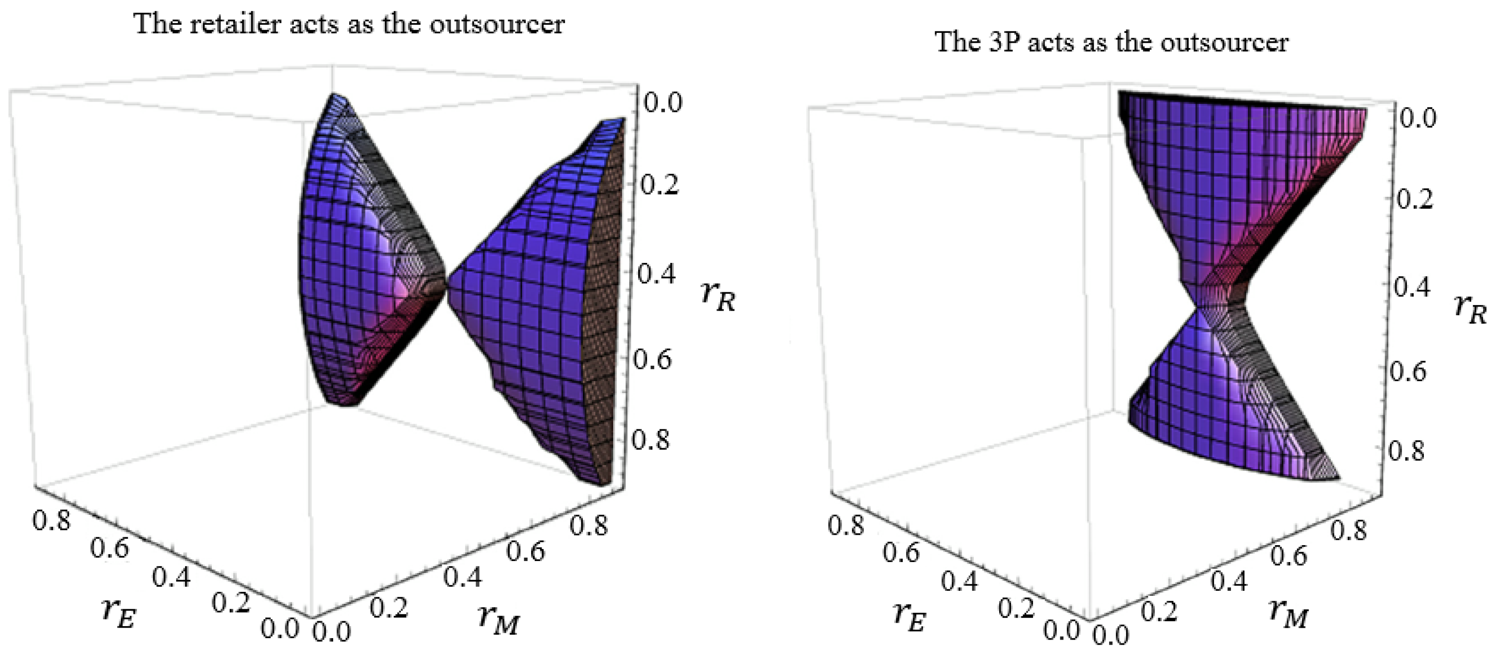
As for the supply side of the market, backward logistics also significantly influence consumer demand, as we concluded from Figure 1, which was generated by the 3-D simulation tool in Matlab. Managing the reverse logistics properly is important as it impacts sales and marketing strategies [13]. From this research, marketing strategies can be viewed as a proxy for the players’ social performance to some extent. Therefore, the manufacturer’s decision for the closed loop supply chain structure will affect the social outcomes. Majumder and Groenevelt [23] also emphasized that remanufacturing and pricing strategies should be determined jointly to increase the efficiency of the loop. As the reverse logistics strategy considerably influence the customers’ desire to return the used product, the reward flows must be handled successfully to appropriately impact sales. From Figure 1, outsourcing this business can increase sales only when the collecting cost of the manufacturer is substantially higher than that of the outsourcer. The cost structure of the chain influences the benefit obtained from the reverse flows, so the customers receive additional pressure when making a purchasing choice when the remanufacturing system is efficient. As such, we concluded that outsourcing is a wise choice, independent of the manufacturer’s collecting costs.

Remark 3.

Considering all admissible parameters, the retailer always benefits when collecting the used product.

Many researchers [1,2,4] are concluding that the retailer always benefits economically when it manages the reverse logistics. Bhattacharya et al. [2] proved that an efficient reverse flow mechanisms will enforce the retailer’s desire to increase the volume of business when it performs better operationally and economically than when the loop is not closed. Collecting the used electronic product is not a traditional task for a retailer who seeks to profit using marketing, pricing, and advertising strategies. When the incentive for collecting the used electronic product is sufficiently high, the retailer invests more to the remanufacturing system and its gains may be even higher than those of the manufacturer. As the leader of the chain, the manufacturer should prioritize choosing the structure of the chain. If the reverse flows managed by the retailer will result in a higher payoff for the manufacturer, then the manufacturer will choose to outsource this business to the retailer who will also benefit.

Finally, we should note that the third-party service provider is always willing to close the loop if asked to perform this operation, as the service provider is paid on a cost-plus basis that will result in incurring a profit. Because the close-loop supply chain will not affect the prices and the demands of the second-period equilibrium, the influence of these three supply chain models on the consumer can only be assessed by sales in the first period.

6. Conclusions

The analysis of the differences in the players’ performances in these three models will help the manufacturer select an optimal method to close the loop to significantly increase its profits. Our results can assist the decision-maker during the selection of a proper reverse logistics structure to efficiently run the chain. This paper also reveals the strategic nature of a closed-loop supply chain in the electronic sector. The theoretical and practical implications are as follows:

Firstly, our research determines that both the retailer and the third-party service provider have considerable interest when they are chosen to manage the reverse logistics flows. The retailer always prefers that the loop is closed, whether or not it is chosen to manage the product collection exclusively. Regardless, the retailer has more control on the forward flows when it can determine the return rate. Because the retailer has additional power in the chain, it is always better off economically, no matter how the reverse logistics are managed. Conversely, a third-party service provider always prefers to manage the reverse logistics exclusively, simply because this is its core business. This evidence introduces some interesting ideas to decision-makers about the implementation of an adequate incentive in the chain.

Secondly, the manufacturer always prefers to select the retailer as the outsourcer to close the loop, only if the third-party service provider operationally performs better than the retailer. Extraordinarily, when both outsources show equal performance operationally, the manufacturer is always willing to outsource this operation to a retailer. We deem that this conclusion is due to the interaction between marketing and operational strategies. Because the retailer also has the opportunity to create a pricing strategy, it decides the price when marketing with the dual target of increasing sales and the return rate. This result provides further information about choosing a proper closed loop supply chain structure, emphasizing the importance of considering the differences between outsource operational performance and the relationships of the chain and the supplier decision power.

Thirdly, these three models demonstrate that the wholesale and retail prices are lower only in the few cases in which the manufacturer chooses to outsource the operation. When the manufacturer does not collect by itself, outsourcers may create speculative strategies that negatively impact their business. This conclusion is particularly relevant for decision-makers when they evaluate the social operation progress for which a specific closed-loop supply chain structure will be required. The choice to outsource reverse logistics significantly influences the pricing strategies and, consequently, the demand.

Though this study has identified some important theoretical and managerial insights, there are several directions worth investigating in further research. Future efforts could consist in investigating the impact of the recovery policy on the whole closed-loop supply chain and its members, where the recycling fraction is a state variable. Secondly, a more complex system with random demand and random return of used electronic products could be considered. Lastly, more comprehensive contracts could also be considered, such as quantity discount contracts and revenue sharing contracts, to the closed-loop supply chain when making decisions.

References

- Savaskan, R.C.; Bhattacharya, S.; Van Wassenhove, L.N. Closed-Loop Supply Chain Models with Product Remanufacturing. Manag. Sci. 2004, 50, 239–252. [Google Scholar] [CrossRef]
- Savaskan, R.C.; Van Wassenhove, L.N. Reverse Channel Design: The Case of Competing Retailers. Manag. Sci. 2006, 52, 1–14. [Google Scholar] [CrossRef]
- Turki, S.; Rezg, N. Unreliable manufacturing supply chain optimisation based on an infinitesimal perturbation analysis. Int. J. Syst. Sci. Oper. Logist. 2016, 5, 25–44. [Google Scholar] [CrossRef]
- Giovanni, P.D. Environmental collaboration through a reverse revenue sharing contract. Ann. Oper. Res. 2014, 6, 1–23. [Google Scholar]
- Mitra, S. Inventory management in a two-echelon closed-loop supply chain with correlated demands and returns. Comput. Ind. Eng. 2012, 62, 870–879. [Google Scholar] [CrossRef]
- Turki, S.; Didukh, S.; Sauvey, C.; Rezg, N. Optimization and Analysis of a Manufacturing–Remanufacturing–Transport–Warehousing System within a Closed-Loop Supply Chain. Sustainability 2017, 9, 561. [Google Scholar] [CrossRef]
- Huang, Z.; Nie, J.; Tsai, S.-B. Dynamic Collection Strategy and Coordination of a Remanufacturing Closed-Loop Supply Chain under Uncertainty. Sustainability 2017, 9, 683. [Google Scholar] [CrossRef]
- Giovanni, P.D.; Zaccour, G. Cost–Revenue Sharing in a Closed-Loop Supply Chain; Birkhäuser: Boston, MA, USA, 2013. [Google Scholar]
- Yoon, S.; Jeong, S. Investment Strategy in a Closed Loop Supply Chain: The Case of a Market with Competition between Two Retailers. Sustainability 2017, 9, 1712. [Google Scholar] [CrossRef]
- Qiang, Q.; Ke, K.; Anderson, T.; Dong, J. The closed-loop supply chain network with competition, distribution channel investment, and uncertainties. Omega 2013, 41, 186–194. [Google Scholar] [CrossRef]
- Maiti, T.; Giri, B.C. A closed loop supply chain under retail price and product quality dependent demand. J. Manuf. Syst. 2015, 37, 624–637. [Google Scholar] [CrossRef]
- Zhang, Z.Z.; Wang, Z.J.; Liu, L.W. Retail Services and Pricing Decisions in a Closed-Loop Supply Chain with Remanufacturing. Sustainability 2015, 7, 2373–2396. [Google Scholar] [CrossRef]
- Miao, S.; Chen, D.; Wang, T. Modelling and research on manufacturer’s capacity of remanufacturing and recycling in closed-loop supply chain. J. Stat. Comput. Sim. 2017, 87, 3325–3335. [Google Scholar] [CrossRef]
- Wu, C.; Wei, Z.; Li, M. Ecological Network Equilibrium Model of Closed-loop Supply Chain of Electronic Information Manufacturing Industry. Sci. Technol. Manag. Res. 2015, 5, 190–194. [Google Scholar]
- Phuc, P.N.K.; Yu, V.F.; Chou, S.Y. Optimizing the fuzzy closed-loop supply chain for electrical and electronic equipments. Int. J. Fuzzy. Syst. 2013, 15, 9–21. [Google Scholar]
- Hong, I.H.; Yeh, J.S. Modeling closed-loop supply chains in the electronics industry: A retailer collection application. Transport. Res. E-Log. 2012, 48, 817–829. [Google Scholar] [CrossRef]
- Li, Q.; Xiao, R.B. Adaptive Coordination of Closed-Loop Supply Chain for Consumer Electronic Product with Uncertainty. Ind. Eng. J. 2013, 4, 20–27. [Google Scholar]
- He, X.; Prasad, A.; Sethi, S.P. Cooperative Advertising and Pricing in a Dynamic Stochastic Supply Chain: Feedback Stackelberg Strategies. Soc. Sci. Elect. Pub. 2009, 18, 1634–1649. [Google Scholar] [CrossRef]
- Debo, L.G.; Toktay, L.B.; Wassenhove, L.N.V. Market Segmentation and Product Technology Selection for Remanufacturable Products. Manag. Sci. 2005, 51, 1193–1205. [Google Scholar] [CrossRef]
- Tsai, S.-B. Using the DEMATEL model to explore the job satisfaction of research and development professionals in China’s photovoltaic cell industry. Renew. Sustain. Energy Rev. 2018, 81, 62–68. [Google Scholar] [CrossRef]
- Lee, Y.-C.; Hsiao, Y.-C.; Peng, C.-F.; Tsai, S.-B.; Wu, C.-H.; Chen, Q. Using Mahalanobis–Taguchi system, logistic regression, and neural network method to evaluate purchasing audit quality. Proc. Inst. Mech. Eng. Part B J. Eng. Manuf. 2015, 229, 3–12. [Google Scholar] [CrossRef]
- Liu, B.; Li, T.; Tsai, S.-B. Low carbon strategy analysis of competing supply chains with different power structures. Sustainability 2017, 9, 835. [Google Scholar] [CrossRef]
- Majumder, P.; Groenevelt, H. Competition in remanufacturing. Prod. Oper. Manag. 2010, 10, 125–141. [Google Scholar] [CrossRef]
- Qu, Q.; Tsai, S.-B.; Tang, M.; Xu, C.; Dong, W. Marine ecological environment management based on ecological compensation mechanisms. Sustainability 2016, 8, 1267. [Google Scholar] [CrossRef]
- Tsai, S.-B.; Yu, J.; Ma, L.; Luo, F.; Zhou, J.; Chen, Q.; Xu, L. A study on solving the production process problems of the photovoltaic cell industry. Renew. Sustain. Energy Rev. 2018, 82, 3546–3553. [Google Scholar] [CrossRef]
- Chin, T.; Tsai, S.-B.; Fang, K.; Zhu, W.; Yang, D.; Liu, R.-H.; Tsuei, R.T.C. EO-Performance relationships in reverse internationalization by Chinese Global Startup OEMs: Social networks and strategic flexibility. PLoS ONE 2016, 11, e0162175. [Google Scholar] [CrossRef] [PubMed]
- Lee, S.-C.; Su, J.-M.; Tsai, S.-B.; Lu, T.-L.; Dong, W. A comprehensive survey of government auditors’ self-efficacy and professional Development for improving audit quality. SpringerPlus 2016, 5, 1263. [Google Scholar] [CrossRef] [PubMed]
- Lee, Y.-C.; Wang, Y.-C.; Chien, C.-H.; Wu, C.-H.; Lu, S.-C.; Tsai, S.-B.; Dong, W. Applying revised gap analysis model in measuring hotel service quality. SpringerPlus 2016, 5, 1191. [Google Scholar] [CrossRef] [PubMed]
- Tsai, S.-B.; Zhou, J.; Gao, Y.; Wang, J.; Li, G.; Zheng, Y.; Ren, P.; Xu, W. Combining FMEA with DEMATEL Models to Solve Production Process Problems. PLoS ONE 2017, 12, e0183634. [Google Scholar] [CrossRef] [PubMed]
- Liu, W.; Wei, Q.; Huang, S.-Q.; Tsai, S.-B. Doing Good Again? A Multilevel Institutional Perspective on Corporate Environmental Responsibility and Philanthropic Strategy. Int. J. Environ. Res. Public Health 2017, 14, 1283. [Google Scholar] [CrossRef] [PubMed]
- Wang, J.; Yang, J.-M.; Chen, Q.; Tsai, S.-B. Collaborative Production Structure of Knowledge Sharing Behavior in Internet Communities. Mob. Inf. Syst. 2016, 2016, 8269474. [Google Scholar] [CrossRef]
- Du, P.; Xu, L.; Chen, Q.; Tsai, S.-B. Pricing competition on innovative product between innovator and entrant imitator facing strategic customers. Int. J. Prod. Res. 2016. [Google Scholar] [CrossRef]
- Liu, W.; Shi, H.-B.; Zhang, Z.; Tsai, S.-B.; Zhai, Y.; Chen, Q.; Wang, J. The Development Evaluation of Economic Zones in China. Int. J. Environ. Res. Public Health 2018, 15, 56. [Google Scholar] [CrossRef] [PubMed]
- Guide, V.D.R., Jr.; Jayaraman, V.; Linton, J.D. Building contingency planning for closed-loop supply chains with product recovery. J. Oper. Manag. 2004, 21, 259–279. [Google Scholar] [CrossRef]
- Guide, V.D.R., Jr.; Wassenhove, L.N.V. The Evolution of Closed-Loop Supply Chain Research. Oper. Res. 2009, 57, 10–18. [Google Scholar] [CrossRef]
- Su, J.F.; Yang, Y.; Yang, T. Simulation of Conflict Contagion in Customer Collaborative Product Innovation. Int. J. Simul. Model. 2015, 14, 134–144. [Google Scholar] [CrossRef]
Figure 1.
The profits of a manufacturer in r-space.