Effects of Non-Stationarity on Flood Frequency Analysis: Case Study of the Cheongmicheon Watershed in South Korea


1
Department of Civil Engineering, Kangwon National University, Chuncheon 24341, Korea
2
Department of Civil Engineering, Chungnam National University, Daejeon 34134, Korea
3
Department of Civil Engineering, Seoul National University of Science and Technology, Seoul 01811, Korea
4
Engineering School of Sustainable Infrastructure and Environment, University of Florida, Gainesville, FL 32611, USA
*
Author to whom correspondence should be addressed.
Sustainability 2018, 10(5), 1329; https://0-doi-org.brum.beds.ac.uk/10.3390/su10051329
Submission received: 12 March 2018
/
Revised: 16 April 2018
/
Accepted: 18 April 2018
/
Published: 25 April 2018
(This article belongs to the Special Issue Impacts of Climate Change on Hydrology, Water Quality and Ecology)
Abstract
:Due to global climate change, it is possible to experience the new trend of flood in the near future. Therefore, it is necessary to consider the impact of climate change on flood when establishing sustainable water resources management policy. In order to predict the future flood events, the frequency analysis is commonly applied. Traditional methods for flood frequency analysis are based on the assumption of stationarity, which is questionable under the climate change, although many techniques that are based on stationarity have been developed. Therefore, this study aims to investigate and compare all of the corresponding effects of three different data sets (observed, RCP 4.5, and 8.5), two different frequency models (stationary and non-stationary), and two different frequency analysis procedures (rainfall frequency first approach and direct discharge approach). As a result, the design flood from the observed data by the stationary frequency model and rainfall frequency first approach can be concluded the most reasonable. Thus, the design flood from the RCP 8.5 by the non-stationary frequency model and rainfall frequency first approach should be carefully used for the establishment of flood prevention measure while considering climate change and uncertainty.
1. Introduction
The sustainable water resources management needs to move beyond conceptual theories and to be carried out by practical approaches when the relationship between hydrology and ecology becomes more important [1,2,3]. As the stress on water-dependent habitats is increasing due to climate change and growing anthropogenic activities [4,5,6,7,8], it is quite obvious that balancing the water needs of people and ecosystems will become a major environmental issue. Therefore, a plan for the sustainable water management should include the potential effects of flood, drought, and degradation of water quality, which may occur in the near future. Furthermore, sustainable water management should provide a healthy environment for ecosystems of a watershed [9,10].
Especially, in addition to drought and water quality degradation, extreme and frequent flood events in a specific region can also have a negative impact on ecosystem. Poff [11] analyzed the ecological response to flooding increased by climate change and suggested that the implementation of non-structural flood management policies is of great necessity. Whipple et al. [12] proposed various flood characteristics using a cluster analysis, such as ecological magnitude, time of occurrence, duration, etc. Predick and Turner [13] also examined the components that have effects on habitat quality and habitat configuration in flood.
According to the IPCC [14], the average of global surface temperature had increased by 0.74 °C during the last 100 years. A general consensus showed that the global warming and change of hydrological cycle will cause the increase of extreme climate events in both frequency and intensity, which will result in more severe flooding, drought, and water quality degradation [15,16,17,18,19]. Another important factor is land use change, which means the increase of impervious layer for urbanization. Apollonio et al. [20] analyzed that flooding areas and land use changes are significantly correlated, and also suggested that the correlation can be negligible in a large basin. Blöschl et al. [21] also suggested that land cover change could affect the impact on flooding and low flows. Land use change will have a significant impact in a short-term analysis while climate change will have a significant impact in a long-term analysis because a specific land use change plan in a long-term aspect is too uncertain. Therefore, in this study, only climate change was considered as a factor affecting the estimation of flood, because one of the objectives of this study is to identify the change of flood magnitude of climate scenarios up to 2100.
For the reasonable prediction of future flood under climate change, a flood frequency analysis is an inevitable tool because most of hydraulic structures are planned based on the design floods. The prediction of flood event is carried out by a frequency model, which is a mathematical description of the statistical characteristics [22]. Therefore, the practical applications are of great importance in order to improve the existing methods for flood frequency analysis when the relationship between hydrology and ecology becomes more important.
Numerous methods, such as empirical method, phenomenological method, dynamic method, and stochastic watershed modelling have been proposed to predict flood quantiles at each return period. The empirical method is one of the most popular methods for engineering design and planning. Thus, many hydrologists have carried out various researches to improve flood frequency analyses [23,24,25,26,27]. The traditional flood frequency analysis was performed under the stationary assumption, which means that floods are the consequence of identically distributed and independent random process. However, Milly et al. [28] insisted that the assumption of stationarity is very questionable. Under climate change, more intensive and frequent heavy rainfall events are expected in the future. Therefore, many studies have pointed out that the traditional flood frequency analysis based on stationarity is less reliable in the future [29,30,31,32,33,34,35]. Many methods for flood frequency analysis using the non-stationary condition have been developed to improve the traditional approach. By summarizing the current approaches, Khaliq et al. [36] suggested that the extremal, r-largest, peaks-over-threshold, and time varying moments methods are effective techniques for non-stationary flood frequency analysis.
Besides, it is also important to discuss the analysis procedure to estimate the design flood. In South Korea, due to the lack of observed discharge, rainfall frequency analysis to estimate design rainfalls at each return period is performed firstly, and then the design rainfall is converted into design flood with the same return period. This procedure sometimes calculates the results different from those directly estimated by the annual maximum flood data. Nevertheless, those studies on these effects are limited.
Therefore, the main purpose of this study is to suggest the appropriateness and uncertainty of the design flood through flood frequency analysis at the Cheongmicheon watershed in South Korea. To do this, 12 cases were considered by combining three types of data set, two frequency models, and two frequency analysis procedures, and compared all of the corresponding design floods. First, the observed data, RCP 4.5, and RCP 8.5 data were used as three types of data set. Second, a stationary frequency model and a non-stationary frequency model using the time-varying moment method for the Generalized Extreme Value (GEV) distribution were used as two frequency models. Also, in order to compare the changes of design flood according to two different frequency analysis procedures, the procedure using rainfall frequency analysis and HEC-HMS model and the procedure using SWAT model and flood frequency analysis were used.
2. Methodology
2.1. Non-Stationary Flood Frequency Analysis
The assumptions of independence and stationarity on the observed data are very important because they can validate the results from flood frequency analysis. However, when the frequency of a particular observed data, such as rainfall or temperature, is too high, these two assumptions cannot be applied because this observed data no longer independent and stationary to the previous observations. Especially, the problem of non-stationarity becomes more significant under the climate change. From the perspective of climate change, the statistical parameters change over time, and finally this trend violates these two assumptions. Nowadays, the assumption of non-stationarity is widely accepted and applied in many studies that are related to the frequency analysis and the hydrological modeling. Studies of non-stationarity based on flow or water level data can be broadly divided into two categories, namely validation of non-stationarity and estimation of model parameter under non-stationarity assumption.
The validity of non-stationarity can be assessed by investigating the presence of monotonic trends using the non-parametric Mann–Kendall (MK) test [37]. It is commonly used to identify a gradual trend of time series. When xi and xk of time series, , are independent, the statistics S and signs are calculated by Equation (1). The statistical hypothesis test is also performed in order to find the p-value using ZMK from Equation (2) and significance level, .
Also, the parameters of the various probability density functions (pdf) under the non-stationary condition can be estimated by the various methods, such as r-largest method, peaks-over-threshold (POT) method, time varying moments method, pooled flood frequency analysis, local likelihood analysis, and quantile regression [36].
In recent studies, the estimation of return period using the non-stationary frequency analysis has been performed. Serinaldi [38] explained the differences between stationary univariate and non-stationary multivariate frequency analyses on the aspect of return period. Also, Read and Vogel [39] suggested that a hydraulic structure planned by traditional return period concept can be failed because average return periods become much more uncertain under non-stationary condition. Obeysekera and Salas [40] also summarized that the conventional approaches of return period, risk, and reliability should not be used for a design of hydraulic structure when non-stationary condition exists. Furthermore, Serinaldi and Kilsby [41] argued that the nonstationary frequency analyses should not only be based on at-site time series but also require additional information and detailed exploratory data analyses and thus suggested that advanced technology needs advanced training to be correctly applied before adopting policies that make nonstationary analyses mandatory. Also, Serinaldi et al. [42] argued that the application of null hypothesis tests to detect non-stationarity in a time series could be flawed. Thus, because the debate over the non-stationary frequency analysis has been continuing, a more accurate and advanced theory should be developed. Therefore, this study considered the time varying moment method among the five methods was used to apply non-stationarity.
In the time varying moment method, the length of time window is different depending on the type of data. In this study, the length of time window are set to 10 years for observed rainfall data, and 50 years for future rainfall data (RCP 4.5 and RCP 8.5). Also, Generalized Extreme Value (GEV) distribution is adopted in this study. GEV distribution under the stationarity assumption uses three parameters. The pdf and the cumulative distribution function of the GEV distribution are represented by Equations (3) and (4), respectively.
where , , and are the location, the scale, and the shape parameters, respectively.
Generally, the MLE method is widely used to reasonably estimate GEV parameters. Because it can be obtained by deriving the likelihood function, the log-likelihood function to GEV distribution is shown in Equation (5).
Meanwhile, GEV distribution under the non-stationary assumption is described by the regression results of each parameter. In this study, and are assumed variables, whereas is assumed to be a constant because this shape parameter is difficult to be estimated reliably [43,44]. Equation (6) is the parameter setting on the non-stationary assumption. Equation (7) is the corresponding log-likelihood function to the non-stationary GEV distribution.
2.2. Comparative Strategy
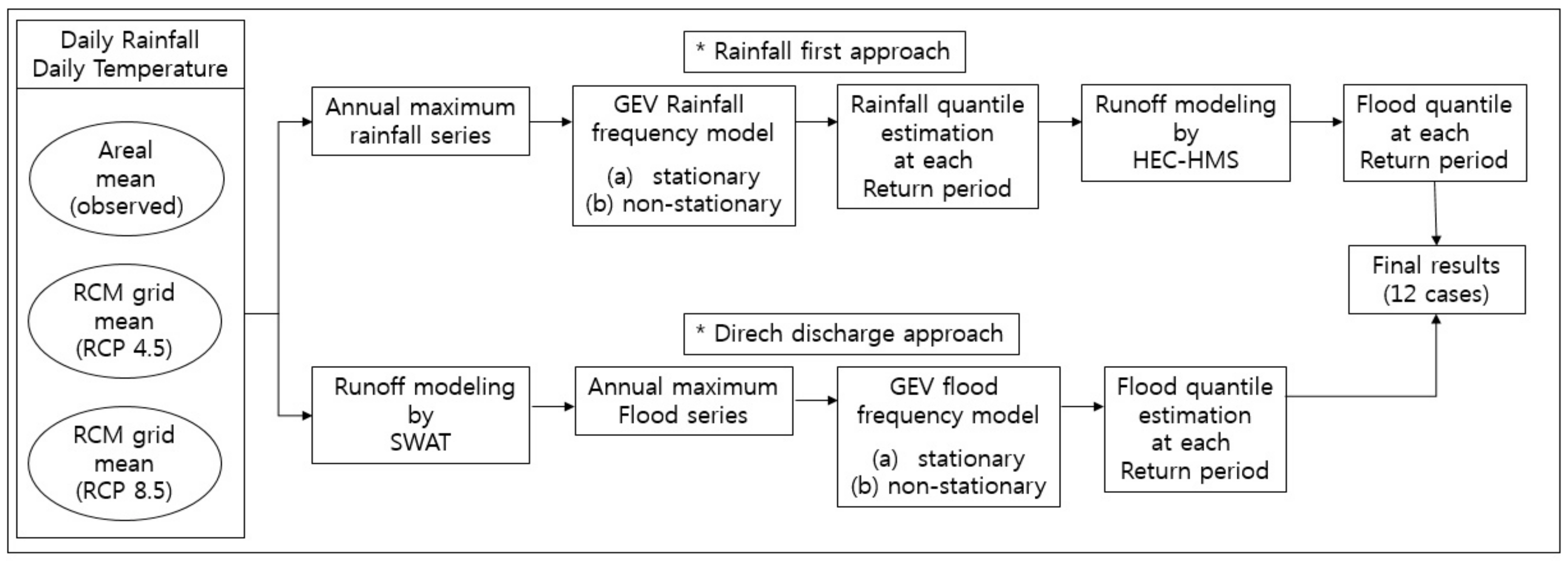
In South Korea, the length of measured discharge data is too short to directly analyze the flood quantiles at each return period. Therefore, the rainfall frequency analysis is firstly performed to calculate the design rainfalls at each return period. Then, the calculated design rainfall is applied to the rainfall-runoff model to estimate the design flood. However, this approach has the disadvantage of using the assumption that the return periods in rainfall and flood are the same. Therefore, the results between this approach (hereafter, rainfall frequency first approach) and the direct flood frequency analysis, which directly uses discharge data (hereafter, direct discharge approach), are compared under stationary or non-stationary flood frequency models using the observed data and the annual maximum rainfall data from RCP 4.5 and 8.5. Figure 1 shows the flowchart of this comparative study.
Firstly, the rainfall frequency analysis under the stationary and non-stationary frequency analyses to the three annual maximum rainfall data (observed, RCP 4.5, and RCP 8.5) are performed, and then the estimated design rainfalls at each return period are input to the Hydrologic Engineering Center-Hydrologic Modeling System (HEC-HMS) to calculate the design flood quantiles. Although there are so many popular software for rainfall-runoff modeling, like MIKE21 [45], SWMM [46], etc., HEC-HMS model (version 4.2) by US Army Corps of Engineers [47] is widely used to simulate the rainfall-runoff process in South Korea. Therefore, the design rainfalls from rainfall frequency analysis can be used to derive design flood quantiles using HEC-HMS.
For the direct discharge approach, the SWAT model that was developed by Arnold et al. [48] has been applied in order to simulate the daily discharge in this study because this model is known as a suitable tool for calculation of daily discharge using daily rainfall data. The hydrological cycle simulated by SWAT model is based on the water balance equation,
where is final soil water content; is the initial soil water content; is the time (days); is the amount of rainfall on a day; is the amount of surface runoff on a day; is the amount of evapo-transpiration on a day; is the amount of infiltrating water on a day; and, is the amount of return flow on a day.
Finally, 12 cases (see Table 1) have been carried out with rainfall frequency first vs direct flood frequency approaches, stationary vs non-stationary frequency models, and three types of available data (observed, RCP 4.5, and RCP 8.5).
2.3. Major Parameters of HEC-HMS Model and Calibration Tool of SWAT Model
After performing the rainfall frequency analysis, the effective rainfall is calculated by the NRCS method. Before the develop HEC-HMS model, the results of the daily design rainfall from rainfall frequency analysis were separated into hourly design rainfall by Huff-3 distributed method. Also, the areal reduction factor, Thiessen polygon method, and critical storm duration concept were used.
The HEC-HMS uses lumped parameters that were averaged in space and time for runoff simulation. The physical information of the sub-basins and reaches were determined using digital elevation model and landuse data. The study watershed was divided into small and relatively homogeneous six sub-basins according to the drainage divides based on the topography (see Figure 1). The CN values of the sub-basin were used to calculate the effective rainfall through the NRCS method, as shown in Table 2. The surface runoff was calculated by Clark hydrograph and the flood routing was conducted by Muskingum method. These values, including time of concentration () and storage coefficient (), are also summarized in Table 2.
In the long-term runoff simulation by SWAT, the most important process is the calibration of model parameters. The modeler’s experience by the trial-and-error method is a popular approach to determine the best set of parameters. However, it is difficult for a modeler to find an optimal parameter value that satisfies the temporal and spatial scales through trial-and-error method. Therefore, a SUFI-2 algorithm in SWAT-CUP tool is used in this study in order to select the appropriate set of parameters for the SWAT model. In SUFI-2, uncertainty in parameters, expressed as ranges, accounts for all the sources of uncertainties such uncertainty in driving variables, conceptual model, parameters, and measured data. The degree of uncertainty is measured by 95% prediction uncertainty (95PPU), here called the P-factor. The results of calibration and validation are shown in Section 4.1.
3. Study Area, Data and Trend Analysis
3.1. Characteristics of Study Area
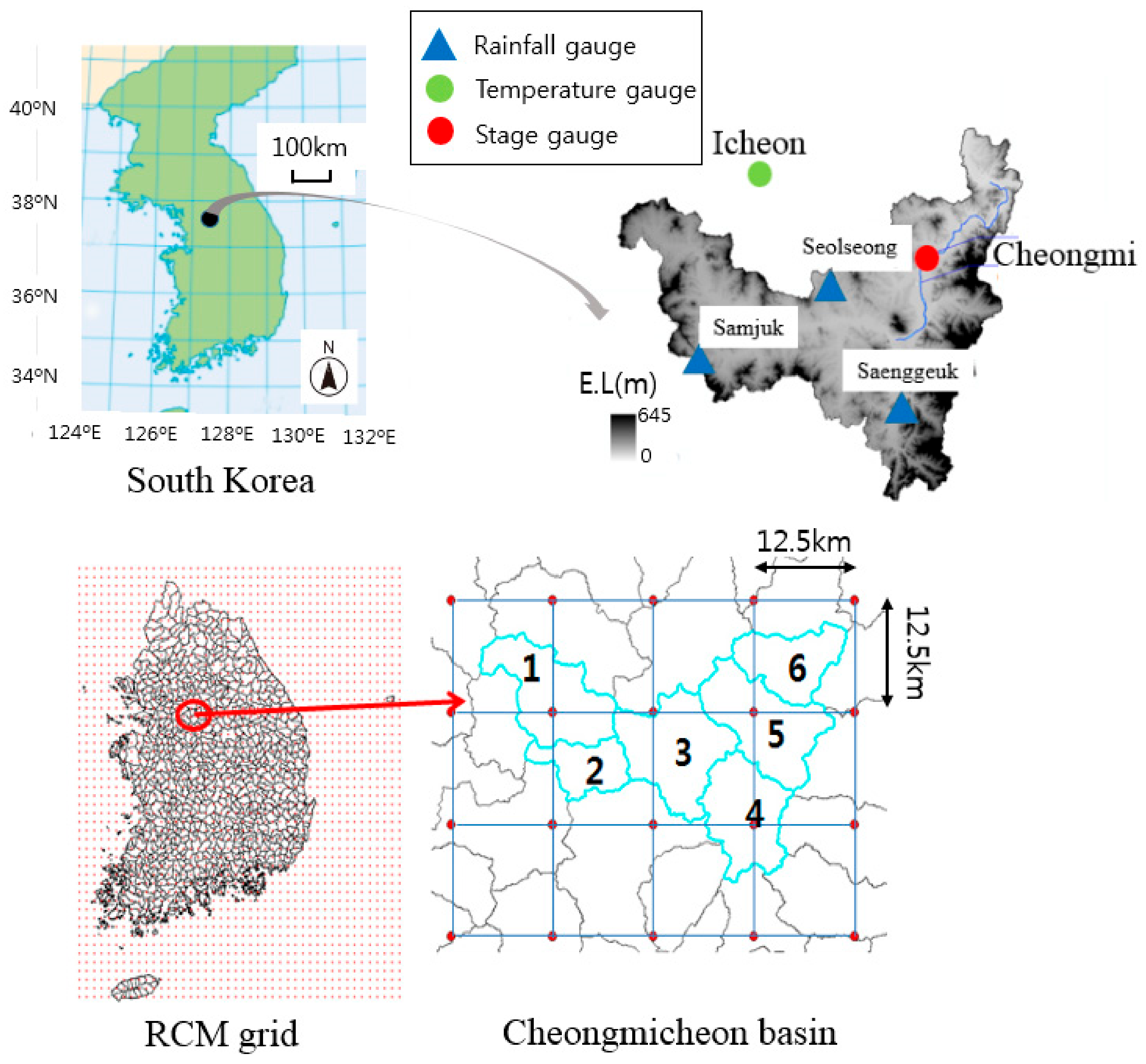
The Cheongmicheon watershed is selected because the water resources management plan preventing flood and drought has been newly developed after Restoration of Four Major Rivers Project funded by South Korea government. The longitude and latitude of this watershed are 127°20′~127°44′ E, and 37°60′~37°84′ N, respectively. The total length of main channel is 60.8 km and the area is 596.60 km2. The mean altitude of the watershed is approximately E.L. 141.38 m, while the altitude of most area lies between E.L. 50 m and E.L. 100 m. The mean gradient is 17.0% with 676 m of the peak altitude. The hydrological soils are categorized as A, B, C, and D by the NRCS method. A type and B type, which are comparatively well drained, account for 5.4% and 33.7% of the total area, respectively, whereas C type and D type, which are comparatively badly drained, account for 17.3% and 43.5% of the total area, respectively. Figure 2 shows the study watershed, which consists of six sub-basins. In this basin, three rain gauges (Seolsung, Samjuk, and Saenggeuk), one temperature gauge (Icheon), and one stage gauge (Cheongmi) are operated.
The meteorological data used in this study are observed and future data. The daily rainfall data and the daily mean temperature data that were measured at three rainfall gauges and a temperature gauge were collected from the stating year of each gauge to 2017. The starting years of Selsong, Samjuk, and Saenggeuk rainfall gauges are 1970, 1990, and 1970, respectively. Also, the starting year of Icheon temperature gauge is 1973.
The future daily rainfall and the future daily mean temperature data were obtained from the regional climate model (RCM), HadGEM3-RO. Representative Concentration Pathways (RCPs) are four greenhouse gas concentration trajectories that were adopted by the IPCC in its fifth Assessment Report in 2014. RCPs are consistent with a wide range of possible change in future anthropogenic greenhouse gas emissions. RCP 2.6 scenario assumes that global greenhouse gas emissions peak between 2010 and 2020 with a substantial decline of emissions thereafter. The maximum emission under RCP 4.5 scenario is expected around 2040 compared with around 2080 under RCP 6.0 scenario. Under the RCP 8.5 scenario, the emissions continue to rise throughout the 21st century. The increase of global greenhouse gas emissions finally increases temperature and precipitation. In this study, RCP 4.5 and 8.5 were selected because these two scenarios were the most representative. The time length of the future data is 90 years from 2011 to 2100.
3.2. Characteristics of the Collected Data and Trend
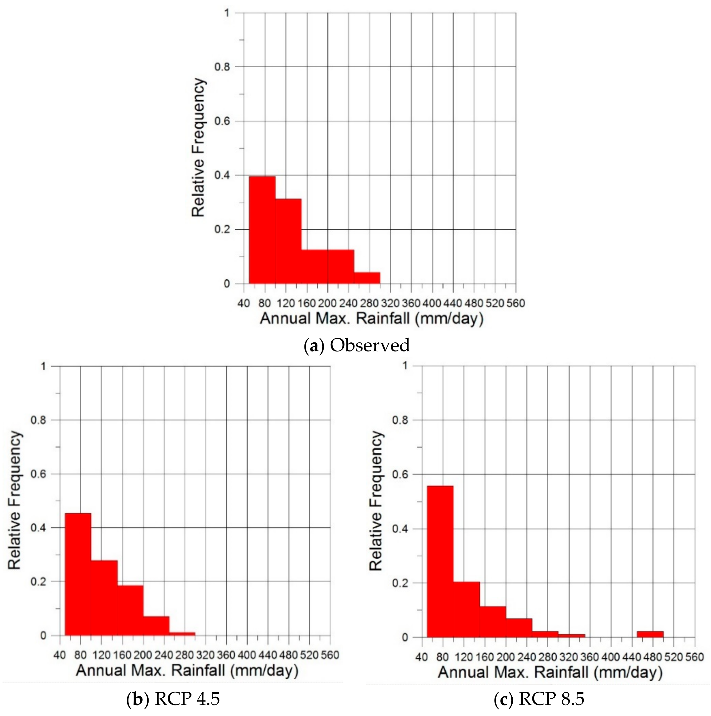
The annual maximum rainfall data sets to the observed and future climate scenarios (RCP 4.5 & 8.5) are shown in Figure 3. Also, Figure 4 and Table 3 show the statistical differences between the observed and the future annual maximum daily rainfall data sets. The probability density of RCP 8.5 is significantly different from those of the observed and RCP 4.5, because the skewness of RCP 8.5 is much larger than others. Also, the probability densities of the observed and RCP 4.5 are similar, but the mean of the observed data is 15.4 mm larger than that of the RCP 4.5.
The MK trend test was performed to identify trends and the results are shown in Table 4. All of the future rainfall data under RCP 4.5 and 8.5 show the weak and strong increasing trends under the 5% significant level, respectively, while the observed data show no trend. Therefore, it can be suggested that non-stationary flood frequency analysis should be considered for the future rainfall data because the stationarity cannot be guaranteed in RCP scenarios.
4. Results
In the rainfall frequency first approaches, the data periods for the past and the future data are 1965 to 2017 and 2011 to 2100, respectively. In the direct discharge approaches, the data periods for the past and future data are 1991 to 2017 and 2011 to 2100. That is, the length of the observed discharge (26 years) is much shorter than that of the observed rainfall (52 years).
4.1. Results of Calibration by HEC-HMS Model and SWAT Model
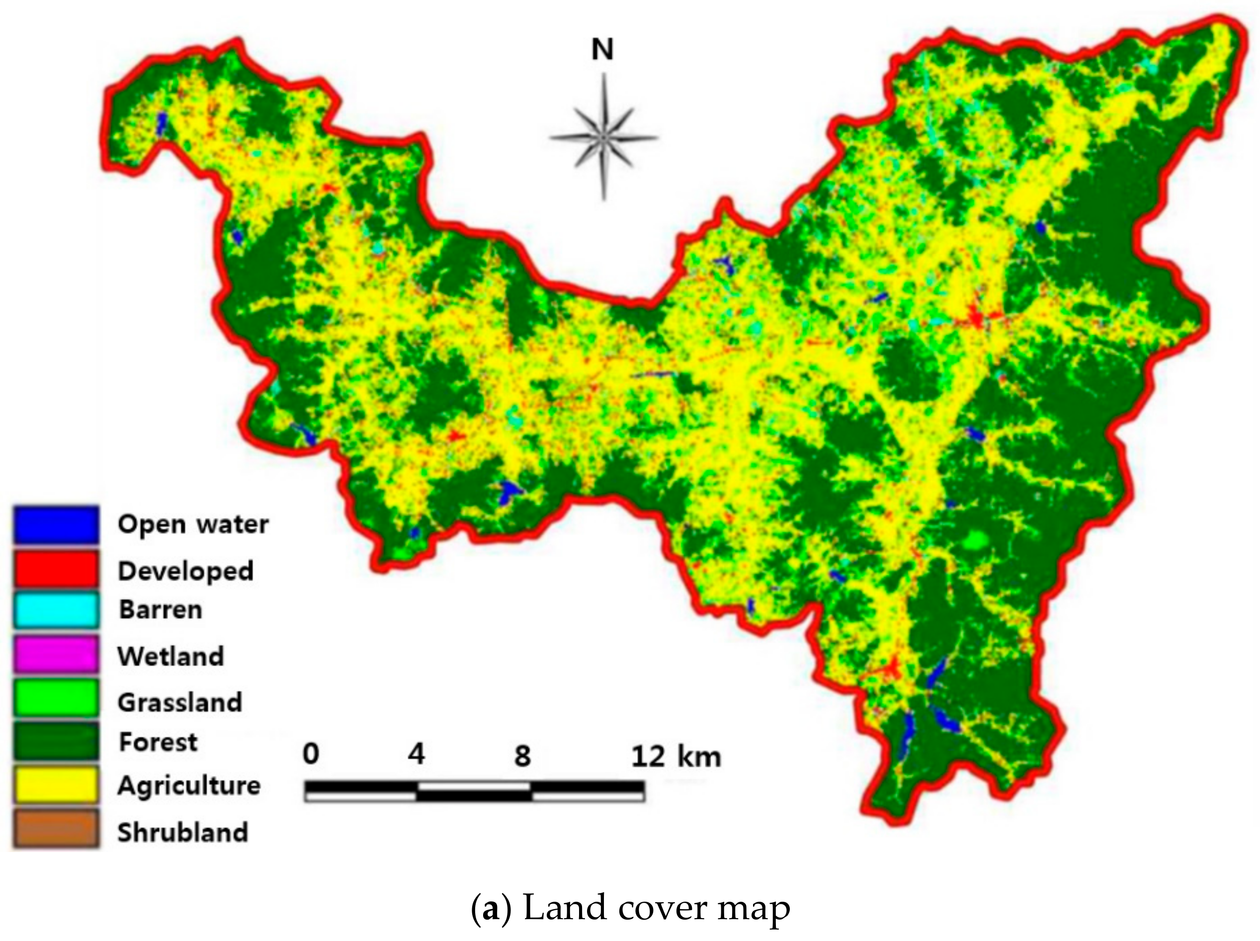
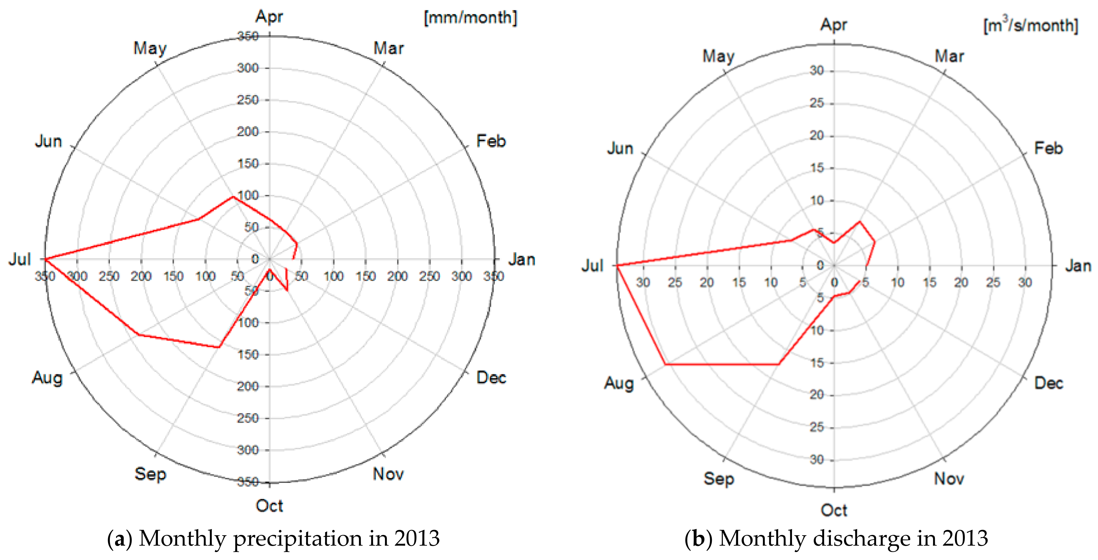
HEC-HMS model is used for the rainfall frequency first approach and SWAT model is adopted for the direct discharge approach. In this study, the case in 2013 is selected to calibrate the parameters using the SWAT model. Figure 5a,b show the land cover map and the soil type map using hydrological soil group by NRCS in the Cheongmicheon watershed. Also, Figure 6a,b represent the monthly precipitation and discharge in 2013. The annual precipitation of the Cheongmicheon watershed in 2013 is 1288 mm/year, while the national average in the Republic of Korea is 1163 mm/year during the same period. 55% of the annual precipitation is concentrated in summer (June to August), while 27% is concentrated in July alone. The annual average discharge is 11.3 m3/s. The greatest monthly discharge occurred in July and the annual maximum daily precipitation is 70 mm, recorded in July. The number of rainy days is 130 and the largest amount of discharge is 157 m3/s.
The parameters in SWAT model were calibrated by SWAT-CUP and also the results were validated. The calibration periods were 1 January 2013–31 December 2013, and also the validation periods were 1 January 1997–31 December 1999. Especially, for the validation, three-year observed daily runoff data was used to check the adequacy of the calibrated parameters in the SWAT model.
Figure 7a,b are the model results of calibration in the year 2013 and validation in the years 1997–1999. With the optimized parameters, the monthly and seasonal discharges are fitted well to the observed. In addition, the Nash and Sutcliffe efficiency (NSE) [49] and R2 are calculated, as shown in Figure 7c. Given that the closer the two indices are to unity, the more accurate the simulation capability of the model is, the model performances can be concluded to be relatively exact.
4.2. Comparative Results of 12 Cases
The probability distribution for frequency analysis of rainfall data and discharge data is a GEV distribution with three parameters in this study. The three parameters of GEV distribution are estimated by MLE, because it is unbiased, consistent, and sufficient estimator to GEV distribution. The time varying moment method with 10-years (observed rainfall data and discharge) and 50-years (future rainfall and discharge under RCPs 4.5 and 8.5) is used to perform the non-stationary frequency analysis. When the rainfall frequency first approach is applied, the design rainfalls at all of the return periods are converted into discharges by the HEC-HMS model. In the case of direct discharge approach, the annual maximum floods that were generated by SWAT model are directly used to perform flood frequency analysis.
Table 5 summarizes the results of the design floods at each return period of 12 cases. At all return periods, RCP 8.5 has the higher values of design flood when compared to RCP 4.5. The standard return period in the Cheongmicheon watershed is 100-year. In 100-year return period, the minimum design flood was 1973.4 m3/s (Case 6), and also, the maximum design flood was 3975.2 m3/s (Case 11). However, using only Table 5, it is very difficult to suggest the most likely design flood in the Cheongmicheon watershed because there is high uncertainty between the cases. Therefore, the impact analyses to combinations of three types of data sets, two types of frequency models, and two types of frequency analysis approaches were performed before the suggestion of the most reasonable design flood.
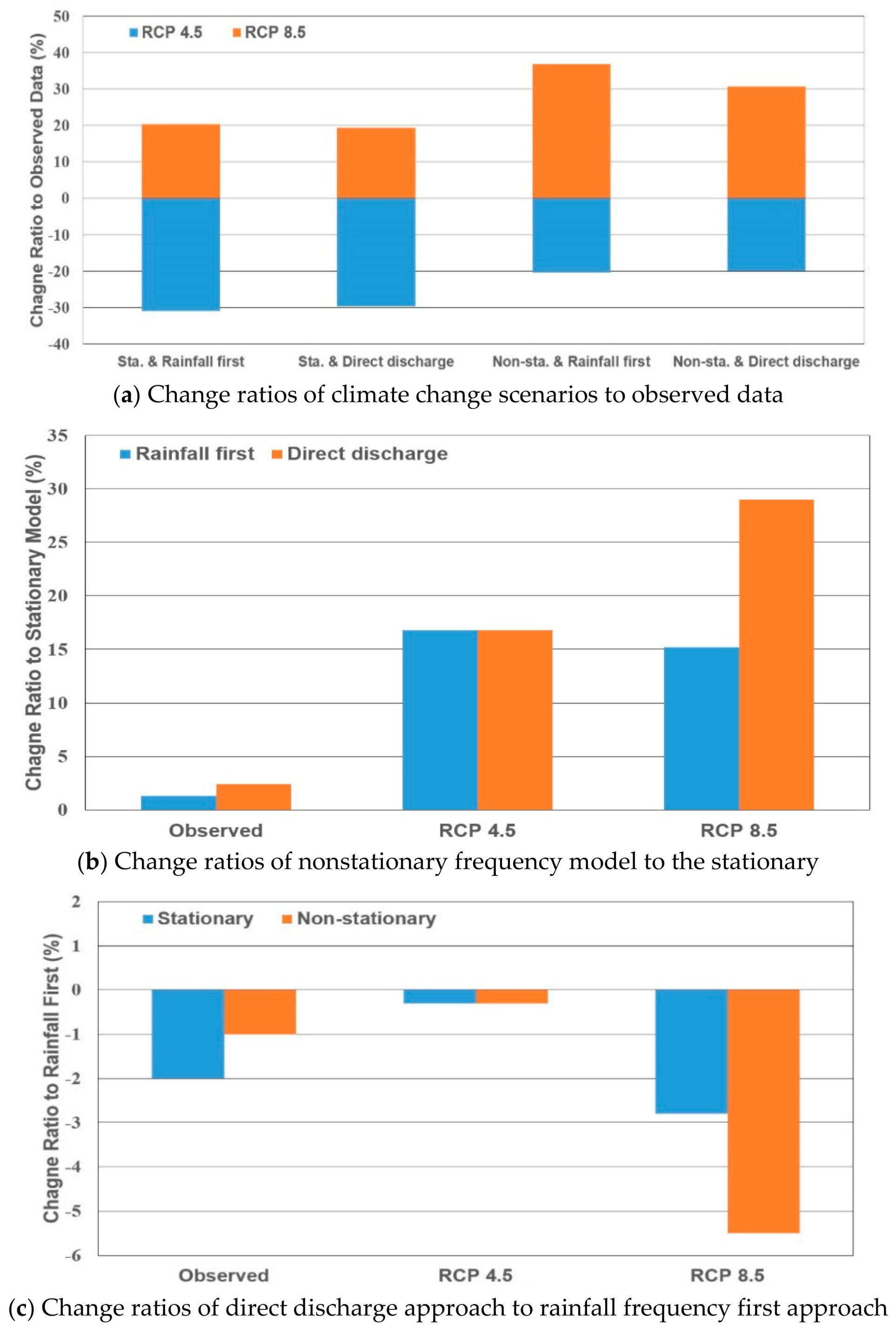
Figure 8a–c show the change ratios to each method. Firstly, in Figure 8a, all of the design floods from the observed data were larger than those from RCP 4.5 and smaller than those from RCP 8.5. Especially, the design flood by the combination between non-stationary frequency model and the rainfall frequency first approach was the highest under RCP 8.5. Therefore, it can be suggested that the design floods from RCP 4.5 are too small to establish the reasonable flood measure in the Cheongmicheon watershed. However, it is very difficult to choose between the design flood from the observed data and RCP 8.5, because RCP 8.5 is a possible scenario in the future. Therefore, it can be suggested that the design floods from the observed data and RCP 8.5 are considered as uncertainty for the effective flood prevention planning.
The second effect on the design floods is a type of the frequency model. Figure 8b shows the change ratios to the stationary frequency model. All of the design floods from RCP 4.5 and 8.5 were lager than those from the observed data. Especially, the difference of the design flood between stationary and non-stationary frequency models on the observed data was much smaller than those of RCP 4.5 and 8.5 because the stationarity in the observed data was valid, as shown in the results of MK test. Therefore, it is suggested that the stationary frequency model is enough to estimate design flood from the observed data but the non-stationary frequency model should be used to estimate it from RCP 8.5.
The last effect is a type of the frequency analysis procedure. Figure 8c shows the change ratios to rainfall frequency first approach. All of the design floods by direct discharge approach were smaller than those of rainfall frequency first approach. However, it is suggested that this effect can be negligible because the maximum change ratio (−5.5%) was significantly smaller than those of the other two effects. Therefore, it is reasonable that the rainfall frequency first approach is selected because it is commonly used in South Korea due to the lack of flood data.
Finally, when comparing all the results of three effects, the 100-year design flood (2866.2 m3/s) from the observed data by the stationary frequency model and the rainfall frequency first approach (Case 1) can be suggested as the most reasonable because climate scenarios has not been applied yet in South Korea. However, it is needed that the 100-year design flood (3975.2 m3/s) from the RCP 8.5 by the non-stationary frequency model and the rainfall frequency first approach (Case 11) should be carefully considered in the future. In spite of ambiguity of selection of reasonable approach these results can be used to develop the mandating flood prevention guideline considering climate change because there has been no standard approach in South Korea.
5. Conclusions
The variability of flood has been significantly impacted by the climate change, and it affects the sustainability of ecological systems, including a human society. Estimation of design flood by frequency analysis is the first step of sustainable water resources management for the prevention of flooding, drought, and degradation of water quality in a watershed. However, the assumption of stationarity used in conventional flood frequency analysis does not consider the increasing variation of rainfall due to climate change. Therefore, in this study, the various factors, including non-stationarity to impact the design flood through flood frequency analysis, were examined at the Cheongmicheon watershed in South Korea.
After data collection at the watershed of interest, trends of observed data, and future data under RCP 4.5 and 8.5 in the Cheongmicheon watershed were investigated by MK non-parametric trend test. The stationarity was less plausible under RCP 4.5 and 8.5 because all future annual maximum daily rainfall data under RCP 4.5 and 8.5 showed the increasing trend. Also, the comparative study using 12 cases combined by three different data sets (observed, RCP 4.5, and 8.5), two different frequency models (stationary and non-stationary), and two different frequency analysis procedures (rainfall frequency first and direct discharge approach) was performed to investigate their impact on the design floods. In two different frequency modeling, the GEV distribution was selected as the probability distribution, and also, the time varying moment method with 10-year for the observed data and 50-year for the RCP 4.5 and 8.5 moving window was applied for the non-stationary frequency analysis. Also, in two different frequency procedures, HEC-HMS model for rainfall frequency first approach and SWAT model that was calibrated by SUFI-2 algorithm for direct discharge approach were used to estimate design flood at each return period.
By analyzing results of the 12 cases, it was known that the design floods from RCP 8.5 (Cases 9, 10, 11, and 12) were relatively larger compared to those from RCP 4.5 (Cases 5, 6, 7, and 8). Especially, the design floods from RCP 4.5 were smaller than those from the observed data (Cases 1, 2, 3, and 4). Therefore, it was concluded that the design floods from RCP 4.5 were excluded firstly in the suggestion of the reasonable design flood. However, on the aspect of uncertainty in climate scenario, it was suggested that the design flood from RCP 8.5 could be considered as a possible one. As a result of effect by different frequency modeling, it was found that all of the design floods using non-stationary frequency model were larger than those using stationary frequency modeling. However, it was suggested that the stationary modeling was only applied to the observed data because the change ratio on the observed data were negligibly small. This result was consistent with the result of MK non-parametric trend test. Also, the results of effect by different frequency procedure showed that this effect could be negligible because the change ratio was significantly small when compared to other effects. Therefore, it was suggested that the rainfall frequency first approach was reasonable because it was generally used in South Korea.
Finally, this study showed that the design floods in Case 1 (observed data + stationary frequency model + rainfall frequency first approach), which is the same to the standard of South Korea were the most reasonable for establishment of flood prevention measure at the Cheongmicheon watershed. However, it can be proposed that the design floods in Case 11 (RCP 8.5 + non-stationary frequency model + rainfall frequency first approach) should be considered as importantly in near future because climate change scenarios have not been applied to frequency analysis yet in South Korea. For the preventive measures, the consideration of climate change and land use change scenarios should be in the calculation process of design floods. In the future, the covariates will be added to this approach to include the effects of additional meteorological and physical information.
Author Contributions
S.U.K. and M.S. established research direction and gave constructive suggestions. E.-S.C. and X.Y. performed the analysis in this study and also wrote this manuscript.
Acknowledgments
This study was supported by Chungnam National University.
Conflicts of Interest
The authors declare no conflict of interest.
References
- Wood, P.G.; David, M.H.; Sadler, J.P. Hydroecology and Ecohydrology: Past, Present and Future; John Wile & Sons: West Sussex, UK, 2007. [Google Scholar]
- Elderd, B.D.; Nott, M.P. Hydrology, habitat change and population demography: An individual-based model for the endangered Cape Sable seaside sparrow ammodramus maritimus mirabilis. J. Appl. Ecol. 2008, 45, 258–268. [Google Scholar] [CrossRef]
- Tilman, D.; Haddi, A.E. Drought and biodiversity in grass land. Oecologia 1992, 89, 257–264. [Google Scholar] [CrossRef] [PubMed]
- Wang, Y.-J.; Qin, D.H. Influence of climate change and human activity on water resources in arid region of Northwest China: An overview. Adv. Clim. Chang. Res. 2017, 8, 268–278. [Google Scholar] [CrossRef]
- Zang, C.; Liu, J.; Jiang, L.; Gerten, D. Impacts of human activities and climate variability on green and blue water flows in the Heihe river basin in Northwest China. Hydrol. Earth Syst. Sci. 2013, 10, 9477–9504. [Google Scholar] [CrossRef]
- Chenoweth, J.; Hadjikakou, M.; Zounides, C. Quantifying the human impact on water resources: A critical review of the water footprint concept. Hydrol. Earth Syst. Sci. 2014, 18, 2325–2342. [Google Scholar] [CrossRef] [Green Version]
- Chung, E.S.; Park, K.; Lee, K.S. The relative impacts of climate change and urbanization on the hydrological response of a Korean urban watershed. Hydrol. Process. 2011, 25, 544–560. [Google Scholar] [CrossRef]
- Kim, H.; Lee, K.-K. A comparison of the water environment policy of Europe and South Korea in response to climate change. Sustainability 2018, 10, 384. [Google Scholar] [CrossRef]
- OECD. Sustainable Management of Water Resources in Agriculture; IWA Publishing: London, UK, 2010. [Google Scholar]
- Kotir, J.H.; Smith, C.; Brown, G.; Marshall, N.; Johnstone, R. A System dynamics simulation model for sustainable water resources management and agricultural development in the Volta river basin, Ghana. Sci. Total Environ. 2016, 15, 444–457. [Google Scholar] [CrossRef] [PubMed]
- Poff, N.L. Ecological response to and management of increased flooding caused by climate change. Philos. Trans. R. Soc. Lond. 2002, 360, 1497–1510. [Google Scholar] [CrossRef] [PubMed]
- Whipple, A.A.; Viers, J.H.; Dahlke, H.E. Flood regime typology for floodplain ecosystem management as applied to the unregulated Cosumnes River of California, United States. Ecohydorlogy 2017, 10, 1–18. [Google Scholar] [CrossRef]
- Predick, K.I.; Turner, G.G. Landscape configuration and flood frequency influence invasive shrubs in floodplain forests of the Wisconsin River (USA). J. Ecol. 2008, 96, 91–102. [Google Scholar] [CrossRef]
- IPCC. Climate Change 2014 Fifth Assessment Report: Synthesis Report; WMO: Geneva, Switzerland; UNEP: Nairobi, Kenya, 2014. [Google Scholar]
- Dastagir, M.R. Modeling recent climate change induced extreme events in Bangladesh: A review. Weather Clim. Extrem. 2015, 7, 49–60. [Google Scholar] [CrossRef]
- Wheaton, E.; Kulshreshtha, S. Environmental sustainability of agriculture stressed by changing extremes of drought and excess moisture: A conceptual review. Sustainability 2017, 9, 970. [Google Scholar] [CrossRef]
- Wamsler, C.; Brink, E. Planning for climatic extremes and variability: A review of Swedish municipalities’ adaptation responses. Sustainability 2014, 6, 1359–1385. [Google Scholar] [CrossRef]
- Won, K.; Chung, E.-S.; Choi, S.-U. Parametric assessment of water use vulnerability variations using SWAT and fuzzy TOPSIS coupled with entropy. Sustainability 2015, 7, 12052–12070. [Google Scholar] [CrossRef]
- Xiao-long, W.; Yong-long, L.U.; Jing-yi, H.A.N.; Gui-zhen, H.E.; Tie-yu, W. Identification of anthropogenic influences on water quality of rivers in Taihu watershed. J. Environ. Sci. 2007, 19, 475–481. [Google Scholar]
- Apollonio, C.; Balacco, G.; Novelli, A.; Tarantino, E.; Piccinni, A.F. Land use change impact on flooding areas: The case study of Cervaro basin (Italy). Sustainability 2016, 8, 996. [Google Scholar] [CrossRef]
- Blöschl, G.; Ardoin-Bardin, S.; Bonell, M.; Dorninger, M.; Goodrich, D.; Gutknecht, D.; Matamoros, D.; Merz, B.; Shand, P.; Szolgay, J. At what scales do climate variability and land cover change impact on flooding and low flows? Hydrol. Process. 2007, 21, 1241–1247. [Google Scholar] [CrossRef]
- Rao, A.R.; Hamed, K.H. Flood Frequency Analysis; CRC Press: Boca Raton, FL, USA, 2000. [Google Scholar]
- Jenkinson, A.F. The frequency distribution of the annual maximum (or minimum) values of meteorological elements. Q. J. R. Meteorol. Soc. 1955, 81, 158–171. [Google Scholar] [CrossRef]
- Alexander, G.N.; Karoly, A.; Susts, A.B. Equivalent distributions with applications to rainfall as an upper bound to flood distribution. J. Hydrol. 1969, 9, 322–373. [Google Scholar] [CrossRef]
- Kirby, W. On the random occurrence of major floods. Water Resour. Res. 1969, 5, 778–784. [Google Scholar] [CrossRef]
- Kuczera, G. Robust flood frequency models. Water Resour. Res. 1982, 18, 315–324. [Google Scholar] [CrossRef]
- Singh, V.P.; Strupczewski, W.G. On the status of flood frequency analysis. Hydrol. Process. 2002, 16, 3737–3740. [Google Scholar] [CrossRef]
- Milly, P.C.D.; Betancourt, J.; Falkenmark, M.; Hirsch, R.M.; Kundzewicz, Z.W.; Lettenmaier, D.P.; Stouffer, R.J. Stationarity is dead: Whither water management? Science 2008, 319, 573–574. [Google Scholar] [CrossRef] [PubMed]
- Kahana, R.; Ziv, B.; Enzel, Y.; Dayan, U. Synoptic climatology of major floods in the Negev Desert, Israel. Int. J. Climatol. 2002, 22, 867–882. [Google Scholar] [CrossRef]
- Prudhomme, C.; Genevier, M. Can atmospheric circulation be linked to flooding in Europe? Hydrol. Process. 2011, 25, 1180–1190. [Google Scholar] [CrossRef] [Green Version]
- Nakamura, J.; Lall, U.; Kushnir, Y.; Robertson, A.W.; Seager, R. Dynamical structure of extreme floods in the US Midwest and the United Kingdom. J. Hydrometeorol. 2013, 14, 485–504. [Google Scholar] [CrossRef]
- Re, M.; Barros, V.R. Extreme rainfalls in SE South America. Clim. Chang. 2009, 96, 119–136. [Google Scholar] [CrossRef]
- Katz, R.W.; Parlange, M.B.; Naveau, P. Statistics of extremes in hydrology. Adv. Water Resour. 2002, 25, 1287–1304. [Google Scholar] [CrossRef]
- Tramblay, Y.; Neppel, L.; Carreau, J.; Kenza, N. Non-stationary frequency analysis of heavy rainfall events in Southern France. Hydrol. Sci. J. 2013, 58, 1–15. [Google Scholar] [CrossRef]
- Lopez, J.; Frances, F. Non-stationary flood frequency analysis in continental Spanish rivers, using climate and reservoir indices as external covariates. Hydrol. Earth Syst. Sci. 2013, 10, 3103–3142. [Google Scholar] [CrossRef]
- Khaliq, M.N.; Ouarda, T.B.M.J.; Ondo, J.C.; Gachon, P.; Bobée, B. Frequency analysis of a sequence of dependent and/or non-stationary hydro-meteorological observations: A review. J. Hydrol. 2006, 329, 534–552. [Google Scholar] [CrossRef]
- Mann, H.B. Nonparametric tests against trend. Econometrica 1945, 33, 245–259. [Google Scholar] [CrossRef]
- Serinaldi, F. Dismissing return periods! Stoch. Environ. Res. Risk Assess. 2015, 29, 1179–1189. [Google Scholar] [CrossRef]
- Read, L.K.; Vogel, R.M. Reliability, return periods, and risk under nonstationarity. Water Resour. Res. 2015, 51, 6381–6398. [Google Scholar] [CrossRef]
- Obeysekera, J.; Salas, J.D. Frequency of recurrent extremes under nonstationarity. J. Hydrol. Eng. 2016, 21, 4016005. [Google Scholar] [CrossRef]
- Serinaldi, F.; Kilsby, C.G. Stationarity is undead: Uncertainty dominates the distribution of extremes. Adv. Water Resour. 2015, 77, 17–36. [Google Scholar] [CrossRef]
- Serinaldi, F.; Kilsby, C.G.; Lombardo, F. Untenable nonstationarity: An assessment of the fitness for purpose of trend tests in hydrology. Adv. Water Resour. 2018, 111, 132–155. [Google Scholar] [CrossRef]
- Coles, S. An Introduction to Statistical Modeling of Extreme Values; Springer: London, UK, 2001. [Google Scholar]
- Katz, R.W. Statistical Methods for Nonstationary Extremes; Springer: New York, NY, USA, 2013. [Google Scholar]
- DHI. MIKE 21 Short Description; Danish Hydraulic Institute: Hørsholm, Denmark, 1995. [Google Scholar]
- USEPA. Storm Water Management Model: User’s Manual Ver. 5.1; National Risk Management Lab. Office of Research and Development: Cincinnati, OH, USA, 2015.
- US Army Corps of Engineers. Hydrologic Modeling System: User’s Manual Ver. 4.2; Hydrologic Engineering Center: Davis, CA, USA, 2016.
- Arnold, J.G.; Srinivasan, R.; Williams, J.R. Large area hydrologic modeling and assessment. Part I: Model development. J. Am. Water Resour. Assoc. 1998, 34, 73–89. [Google Scholar]
- Nash, J.E.; Sutcliffe, J.V. River flow forecasting through conceptual models: Part I: A discussion of principles. J. Hydrol. 1970, 10, 283–290. [Google Scholar] [CrossRef]
Figure 1.
Flowchart for comparative study.

Figure 2.
Configuration map of the study area and grid map in regional climate model (RCM).

Figure 3.
Annual maximum rainfall data (observed and future).

Figure 4.
Probability densities of annual maximum daily rainfall data sets.

Figure 5.
Land cover and soil type map in the Cheongmicheon watershed.


Figure 6.
Monthly precipitation and discharge in calibration year, 2013.

Figure 7.
Performance results of calibration and validation.

Figure 8.
Summary of change ratios of three approaches.


Table 1.
Comparative 12 cases in this study.
| Cases | Data | Frequency Model | Approach |
|---|---|---|---|
| Case 1 | Annual maximum rainfall data (observed) | Stationary | Rainfall first |
| Case 2 | Direct discharge | ||
| Case 3 | Non-stationary | Rainfall first | |
| Case 4 | Direct discharge | ||
| Case 5 | Annual maximum rainfall data (RCP 4.5) | Stationary | Rainfall first |
| Case 6 | Direct discharge | ||
| Case 7 | Non-stationary | Rainfall first | |
| Case 8 | Direct discharge | ||
| Case 9 | Annual maximum rainfall data (RCP 8.5) | Stationary | Rainfall first |
| Case 10 | Direct discharge | ||
| Case 11 | Non-stationary | Rainfall first | |
| Case 12 | Direct discharge |
Table 2.
Values of physical information and hydrologic parameters for Hydrologic Engineering Center-Hydrologic Modeling System (HEC-HMS) model.
Table 2.
Values of physical information and hydrologic parameters for Hydrologic Engineering Center-Hydrologic Modeling System (HEC-HMS) model.
| Sub-Basins | Area (km2) | CN (AMC III) | Clark’s Method | |
|---|---|---|---|---|
| 1 | 112.65 | 57.007 | 3.31 | 4.50 |
| 2 | 50.551 | 58.489 | 2.07 | 2.40 |
| 3 | 121.332 | 62.116 | 2.89 | 3.49 |
| 4 | 98.328 | 49.743 | 1.94 | 2.56 |
| 5 | 117.44 | 56.852 | 1.93 | 2.42 |
| 6 | 89.381 | 53.708 | 1.88 | 2.09 |
Table 3.
Descriptive statistics of annual maximum daily rainfall data sets.
| Items | Mean (mm) | Std. (mm) | Skewness | Kurtosis | |
|---|---|---|---|---|---|
| Annual maximum rainfall data | Observed | 132.1 | 54.4 | 0.841 | 2.815 |
| RCP 4.5 | 116.7 | 52.4 | 0.798 | 3.010 | |
| RCP 8.5 | 128.3 | 94.1 | 3.096 | 14.495 | |
Table 4.
Results of Mann-Kendall test to the annual maximum rainfall data ( = 0.05).
| Items | p-Value (Rainfall) | Decision (Rainfall) | |
|---|---|---|---|
| Annual maximum rainfall data | Observed | 0.1944 | No trend |
| RCP 4.5 | 0.0436 | Increasing Trend | |
| RCP 8.5 | 0.0097 | Increasing Trend | |
Table 5.
Results of design floods at each return period.
| Cases | 10-year R.P. (m3/s) | 50-year R.P. (m3/s) | 100-year R.P. (m3/s) | 200-year R.P. (m3/s) |
|---|---|---|---|---|
| Case 1 | 776.8 | 1265.2 | 2866.2 | 3198.2 |
| Case 2 | 683.6 | 1253.1 | 2807.8 | 3133.7 |
| Case 3 | 1136.7 | 1781.9 | 2903.6 | 3554.7 |
| Case 4 | 1134.3 | 1763.0 | 2875.1 | 3263.9 |
| Case 5 | 516.1 | 963.7 | 1979.2 | 2153.4 |
| Case 6 | 507.6 | 959.0 | 1973.4 | 2128.4 |
| Case 7 | 829.4 | 1288.0 | 2312.1 | 2495.4 |
| Case 8 | 823.1 | 1278.4 | 2304.1 | 2492.1 |
| Case 9 | 990.3 | 1616.1 | 3451.1 | 4207.1 |
| Case 10 | 831.0 | 1520.2 | 3353.6 | 3829.8 |
| Case 11 | 1617.7 | 2670.6 | 3975.2 | 5584.1 |
| Case 12 | 1516.8 | 2176.6 | 3757.4 | 4732.6 |
© 2018 by the authors. Licensee MDPI, Basel, Switzerland. This article is an open access article distributed under the terms and conditions of the Creative Commons Attribution (CC BY) license (http://creativecommons.org/licenses/by/4.0/).
Share and Cite
MDPI and ACS Style
Kim, S.U.; Son, M.; Chung, E.-S.; Yu, X. Effects of Non-Stationarity on Flood Frequency Analysis: Case Study of the Cheongmicheon Watershed in South Korea. Sustainability 2018, 10, 1329. https://0-doi-org.brum.beds.ac.uk/10.3390/su10051329
AMA Style
Kim SU, Son M, Chung E-S, Yu X. Effects of Non-Stationarity on Flood Frequency Analysis: Case Study of the Cheongmicheon Watershed in South Korea. Sustainability. 2018; 10(5):1329. https://0-doi-org.brum.beds.ac.uk/10.3390/su10051329
Chicago/Turabian StyleKim, Sang Ug, Minwoo Son, Eun-Sung Chung, and Xiao Yu. 2018. "Effects of Non-Stationarity on Flood Frequency Analysis: Case Study of the Cheongmicheon Watershed in South Korea" Sustainability 10, no. 5: 1329. https://0-doi-org.brum.beds.ac.uk/10.3390/su10051329
Note that from the first issue of 2016, this journal uses article numbers instead of page numbers. See further details here.