Characterizing Drought Effects on Vegetation Productivity in the Four Corners Region of the US Southwest

Abstract

The droughts striking the Colorado Plateau, where the Hopi Tribe and Navajo Nation Native American reservation lands are located, and their impacts have appeared slowly and relatively unnoticed in conventional national drought monitoring efforts like the National Drought Monitor. To understand the effect of drought-based drivers on vegetation productivity in the Hopi Tribe and Navajo Nation reservation lands, an assessment approach was developed integrating climate, land cover types, and topographical data with annual geospatially explicit normalized difference vegetation index (NDVI)-related productivity from 1989 to 2014 derived from 15-day composite multi-sensor NDVI time series data. We studied vegetation–environment relationships by conducting multiple linear regression analysis to explain the driver of vegetation productivity changes. Our results suggest that the interannual change of vegetation productivity showed high variability in middle elevations where needleleaf forest is the dominant vegetation cover type. Our analysis also shows that the spatial variation in interannual variability of vegetation productivity was more driven by climate drivers than by topography ones. Specifically, the interannual variability in spring precipitation and fall temperature seems to be the most significant factor that correlated with the interannual variability in vegetation productivity during the last two and a half decades.

1. Introduction

Droughts are a recurrent part of our climate and are considered one of the most complex and least understood phenomenon among all-natural hazards in terms of their impact on vegetation function [1,2,3,4]. In recent years, droughts have become more frequent and severe across the world, with a noticeable increase in their spatial extent [5,6,7]. Droughts threaten societies at different economic, social, and environmental scales [8], and have been recognized as the principal cause of crop loss and severe food shortages, particularly in developing countries [7]. For the past few decades, droughts have constantly threatened the world’s food security [7]. In addition to the economic damage and impacts on natural resources, droughts have severe societal consequences causing displacement and migration and even political unrest [7,8,9].

Droughts in the United Sates are the costliest weather-related disaster [10]. From 1980 to 2003, the cost of drought was estimated at more than $144 billion dollars [11]. In the southwestern United States, droughts are relatively a familiar phenomenon (Figure 1), due to land surface–ocean interactions [12]. Several studies have shown that both climate and human activities are the key driving forces of change in the American Southwest landscapes [13]. Assessment of vegetation response to droughts in the region remains difficult due to the human dimensions of this problem and the changing characteristics of drought [14]. In the southwestern United States, the severity of drought impacts on forested land have been well documented since the 1990s because of temperature increase recorded during this period [14,15,16]

Understanding the spatial and temporal dimensions of droughts in relation to climatological, oceanic, and atmospheric parameters is key for developing drought monitoring tools and to providing valuable information for better early warning and knowledge-based decision support systems to help mitigate their impacts [8,17]. Therefore, effective drought monitoring systems would take into consideration past and present climatological conditions and changes [17]. Monitoring drought patterns and their impacts on vegetation activities and productivity at different spatial and temporal scales still presents some challenges, due in part to the complex relationship between vegetation, environmental, and biophysical factors [4,18].

The Hopi Tribe and Navajo Nation lands, also known as the Four Corners Region, collectively cover over 77,699 km² of land area. The ongoing drought impacting the Colorado Plateau, where the Hopi and Navajo Nation are located, have appeared slowly and relatively unnoticed in conventional national drought monitoring efforts like the National Drought Monitor [19]. The most recent drought conditions (Figure 2) in the region have emerged rapidly and intensely, characterized in 2002 by peak drought conditions. They have remained for well over a decade [4,14,16,19] and will have multiple impacts, not only on economic activity but also on the ecosystem services [12,20]. One concern about the ongoing drought in the region is the storage capacity of the Colorado River and the overuse of the regional aquifers [21].

Assessment of the ongoing drought impacts on the Hopi and Navajo Nation area presents some difficulties due to lack of long-term hydro-climatological data and ecological monitoring observations. This has made it difficult to track, measure, and quantify the impacts through this most recent drought, creating a challenging situation for resource managers and decision makers. The numerous gaps and inconsistencies in the hydro-climatological data make the traditional climate-based drought monitoring strategies based on historical ground-based meteorological observations from the limited existing weather stations not ideal for this region.

The aim of this study is to evaluate and understand the potential drought drivers that have shaped the spatial–temporal variability in vegetation productivity in the region over the period of 1989–2014, and to provide valuable spatial information related to interannual variability and changes in vegetation productivity for planning and mitigation purposes, assisting managers and decision makers in maintaining biodiversity. To address these questions, we developed an assessment approach integrating seasonal climate, land cover types and topographical data with annual geospatially explicit normalized difference vegetation index (NDVI)-related productivity from 1989 to 2014 derived from 15-day composite multi-sensor NDVI time series data. All data sets used in the study were harmonized into 5.6 km spatial resolution to match the NDVI data.

2. Study Area and Data

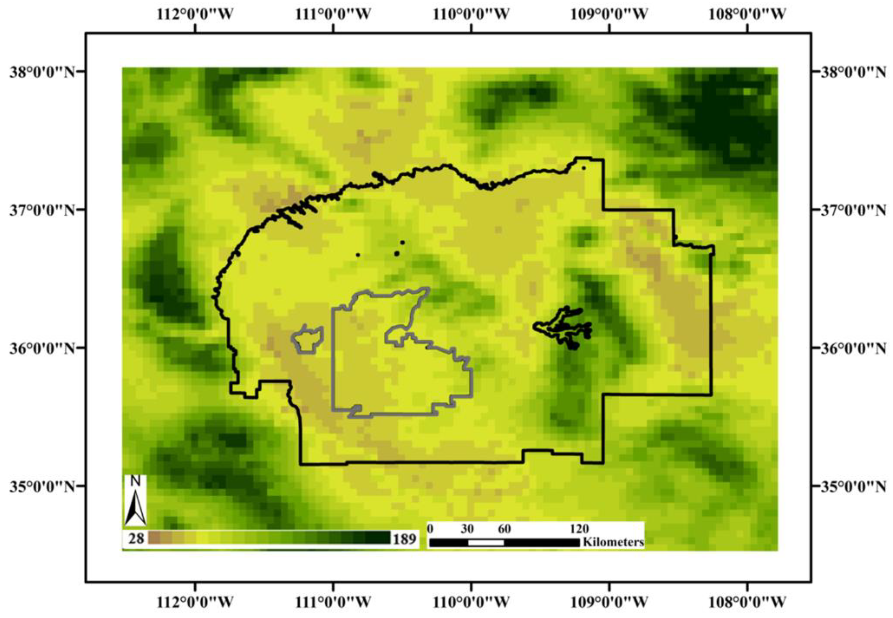
2.1. Study Area

The Hopi and Navajo Nation stretch from the Four Corners Monument landmark across the Colorado Plateau into Arizona, Utah, and New Mexico. The area is known for its cold winters and very hot summers (Figure 3) and its north–south precipitation contrasts. The total annual precipitation is almost equally divided between summer monsoons and winter snow storms. The annual freeze-free period varies between 130 and 180 days. Annual precipitation varies between 127 mm in the southern lower elevations and 381 mm in the higher northern Pinyon-juniper woodland areas atop Black Mesa plateau. Rainfall is low and moderate in the early winter, increases in February and March, and then decreases quickly in April. May through June is a very dry period [22]. Vegetation gradients are further controlled by the bi-seasonal and north–south climatic gradients. Three major cover types can be found in the study area: (1) grass-shrub at altitudes below 1650 m mainly dominated by sparse grassland-browse types of vegetation; (2) Pinyon-juniper between 1650 m and 2300 m dominated by woodland-browse species; and (3) pine forest above 2300 m.

2.2. Datasets

2.2.1. Remote Sensing Data

Fifteen-day composite multi-sensor NDVI time series data were acquired from the Vegetation Index and Phenology Laboratory at the University of Arizona for the period 1989 to 2014 at 5.6 km spatial resolution. This product is a sensor-independent and continuous NDVI record derived from AVHRR (1981–1999), SPOT (1998–2002), and MODIS (2000–2014) [23,24]. This 26-year NDVI time series consists of 15-day composites, resulting in 624 temporal images. Detailed information on the datasets is available on the Vegetation Index and Phenology Laboratory website: https://vip.arizona.edu/VIP_MEaSUREs_Project.php.

Climate data, precipitation and temperature, used in the study were generated from Oregon State University’s Parameter-elevation Regressions on Independent Slopes Model (PRISM) [25] dataset at 4 km spatial and monthly temporal resolution. Average seasonal monthly precipitation and temperature data were generated for the period 1989–2014 and were resampled to the NDVI spatial resolution of 5.6 km. As the land cover of the region is fairly stable due to the little natural and anthropogenic changes, the 2005 North American land Cover product at 250 m spatial resolution was used to extract the main land cover types. The land cover database was created by the North American Land Change Monitoring System [26]. According to this dataset, the land of the Hopi tribe and Navajo Nation is mainly characterized by shrubland, grassland, and needleleaf forest (Figure 4b). The pixel size of the land cover types was resampled to 5.6 km, using the dominant class approach, to match the NDVI pixel size. Topographic data used in the study are based on the Advanced Spaceborne Thermal Emission and Reflection Radiometer (ASTER) Global Digital Elevation Model (GDEM). Elevations range between 821 m and 3771 m (Figure 4a) corresponding to ecological zones with sparse to high vegetation cover (Figure 4b). The pixel size of the DEM data was also resampled to 5.6 km to match the NDVI time series.

3. Methodology

To understand the main forces driving changes in vegetation productivity during the last two and a half decades, a five-step framework was proposed and developed using response and explanatory variables approach. The first step is to derive the integrated annual NDVI parameter, a measure of vegetation productivity, as the dependent response variable. The second step consists of selecting the appropriate set of potential explanatory variables by testing the near-linear dependencies among the explanatory variables. This test allows the determination of the multicollinearity levels between the variables and selection of the appropriate explanatory variables as well as to estimate the effects of individual explanatory variables. The third step is to examine the coefficient of variation (CoV) of the productivity variable (response variable) as the ratio of the standard deviation and the spatial mean at the regional and among vegetation communities. The fourth step is to conduct stepwise multiple linear regression analysis (SMLR) to explain the source of the variability and change in vegetation productivity. Finally, the last step is to evaluate the local regression model performance using overall model residuals.

3.1. Response Variable: Deriving Annual Metric of Vegetation Productivity

The integrated annual NDVI (∑NDVI), a proxy of Gross/Net Primary Production (GPP/NPP) productivity parameter (Figure 5) was computed for each year from 1989 to 2014 using the 15-day NDVI time series. The integrated annual NDVI is a reliable proxy of biomass production [27,28] and is an integrative descriptor of ecosystem functioning and environmental drivers. To mitigate background noise, we only extracted these metrics during the snow-free period from March to November of each year to minimize snow impacts on NDVI values [4,29] we further considered NDVI > 0 only.

3.2. Explanatory Variables

The potential explanatory variables assumed to be the key drivers of vegetation productivity change are: climate variables, vegetation types, and topography characteristics.

Table 1. Explanatory variables used in this study including climate and topography drivers. Climate data were divided into the standard four seasons: winter (JFM: January, February, and March), spring (AMJ: April, May, and June), summer (JOS: July, August, and September), and fall (OND: October, November, and December).

Variables	Derived Variables
Topographical characteristics	Elevation Aspect Slope
Climate data	Seasonal precipitation Seasonal temperature
Vegetation types	Vegetation communities

lists the potential different variables used to explain changes in vegetation productivity [30].

3.3. Detecting Multicollinearity among the Explanatory Variables

The overall goal of conducting a multicollinearity test is to assess high intercorrelations among the explanatory independent variables and to remove these highly correlated explanatory variables from the model. Addressing multicollinearity is fundamental to accurately estimate the effects of individual explanatory variables in the regression model. Several techniques are available to detect multicollinearity in multiple regression analyses, such as eigensystem analysis [31,32], condition number technique, and the examination of correlation matrix. For this study, the examination of correlation matrix of explanatory variables was selected to determine the degree of correlation between the explanatory variables. This method is widely used to detect multicollinearity issues in multiple regression models [33,34].

Fourteen explanatory variables were selected for this test: 3 topography-based factors, elevation, slope, and aspect, one vegetation type variable, 10 climate-based variables (8 seasonal precipitation and temperature-based variables, 1 total annual precipitation, and 1 average annual precipitation). Climate data were divided into the standard four seasons. We calculated the seasonal precipitation by accumulating precipitation over the considered period and seasonal temperature by averaging over the same period. Two variables were excluded from the potential explanatory list, annual cumulative and mean annual rainfall, due to their high multicollinearity with other seasonal precipitation variables.

3.4. Interannual Variability of NDVI-Related Productivity Parameter

The interannual coefficient of variation (CoV) has been used to study spatiotemporal variation in vegetation productivity in different climate and ecosystem zones [35,36]. Change in CoV at any given pixel and over any considered period indicates changes in vegetation productivity [35]. For this reason, the use of CoV in this study can be useful to track variations in vegetation productivity. The interannual CoV of productivity was generated for each pixel in the study area to detect spatial difference in vegetation productivity changes along elevation gradients as well as among vegetation communities. Boxplots [37] were used to analyze variations in the interannual CoV of the productivity parameter among vegetation communities.

3.5. Vegetation Productivity–Environment Relationships

Stepwise multiple linear regressions were used to study the relationship between interannual variability in vegetation productivity and the various environmental variables. To determine the long-term responses of vegetation productivity to environmental variables, a spatial–temporal relationship model was developed. This requires bringing all variables into one spatial model to express the variability and change in productivity as a function of environmental variables over 26 years and the whole area as well as among vegetation communities. Residuals from the models were analyzed to infer any possible explanations related to the weakness of the model and if there were other factors that might be the source of the weakness.

4. Results and Discussion

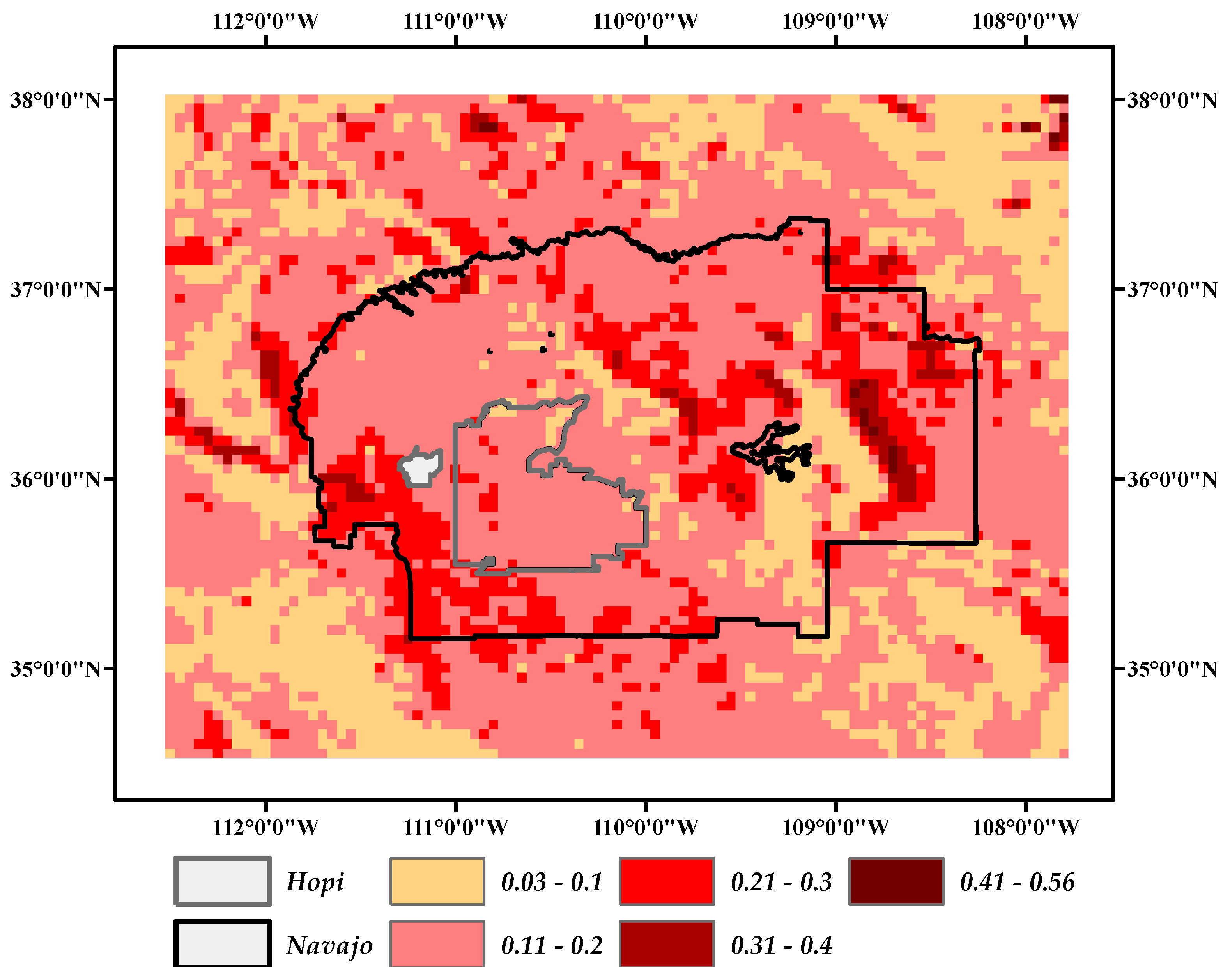
4.1. Spatial Patterns of Interannual CoV of the Productivity Variable

Figure 6 shows the spatial distribution of the interannual CoV of cumulative NDVI over the study period. The lowest interannual CoV values (i.e., those less than 0.1) were concentrated along high elevations indicating that these areas had the most stability and least temporal changes over the study period. These areas are dominated by needleleaf forest. The interannual CoV generally increased with decreasing elevation. The range from 0.21 to 0.56 corresponds to the highest interannual variability, a sign of a greater variability and change in vegetation productivity. The areas corresponding to the highest interannual CoV values are mostly low to mid-elevation where shrubland is the dominant vegetation type. The boxplot in Figure 7 shows the interannual CoV of cumulative NDVI across these three dominant vegetation cover types in the area: needleleaf forest, shrubland, and grassland. The figure indicates that needleleaf forest shows least variability in comparison with shrublands and grasslands. This suggests that needleleaf forest productivity is less sensitive to ongoing droughts, and that shrubland and grassland are more sensitive. This is likely related to the level of resilience among these vegetation communities modulated by their deeper rooting systems and access to deeper water during drought episodes and during the dry season.

4.2. Vegetation Productivity as a Function of Environmental Drivers

The interannual spatial variation in vegetation productivity was analyzed as a function of 12 environmental drivers to explain the source of the variation. The contribution of the potential explanatory variables to the interannual variability in vegetation productivity differed across variables. The results of the multiple linear regression approach used to assess the main forces driving variability in vegetation productivity are listed in

Table 2. Statistical results of the stepwise regression model for the response variable (vegetation productivity) showing the estimated error, standard error, and p-value for the statistical significance explanatory variables (p-value < 0.05).

Explanatory Variables	Estimated Coefficient	Standard Errors	p-Value
Fall precipitation	−0.22	0.018	5.82 × 10−35
Fall temperature	1.08	0.17	7.93 × 10−12
Spring precipitation	0.13	0.02	1.003 × 10−11
Summer precipitation	−0.164	0.015	2.23 × 10−26
Summer temperature	−0.68	0.18	0.005
Winter precipitation	0.05	0.014	1.69 × 10−4
Winter temperature	−0.69	0.087	4.72 × 10−13
Aspect	−0.0001	9.07 × 10−6	1.36 × 10−36
Elevation	−8.58 × 10−5	5.47 × 10−6	3.1 × 10−52
Vegetation types	0.001	4.82 × 10−4	4.56 × 10−5
Whole model	Intercept = 0.48 RMSE = 0.002 Adjusted R-Square = 0.37 p-value = 1.51 × 10−171

. The proportion of the interannual variability in vegetation productivity explained by the potential explanatory variables was around 37%. All explanatory variables, except slope and spring temperature, show a significant correlation at 95% confidence level in the study area. Spatial variation in interannual change in vegetation productivity was explained better by climate drivers than by topography. The interseasonal variability of temperature seems to be the most important factor affecting the vegetation productivity in the area.

Among all explanatory variables, winter and spring precipitation and fall temperature interannual variability showed strong negative impacts on vegetation productivity. Winter and summer temperature, summer and fall precipitation, as well as the topography factors (aspect and elevation) were negatively correlated with productivity, indicating that the interannual variability in vegetation productivity decreases with increase in the factor. These findings suggest that there is a strong positive feedback between the interannual variability in vegetation productivity and winter and fall precipitation, and fall temperature in the area driven by a strong water demand early in the growing season and a potentially longer growing season moderated by a delayed winter temperature both characteristic of cold weather in the region. Furthermore, topographic and vegetation types showed weak correlation coefficients in the regression model and elevation and vegetation types showed decreasing relationship with the interannual variability in cumulative NDVI.

To better understand the uncertainty resulting from the spatial regression model between the interannual variability in response and explanatory variables, the spatial distribution of the regression residuals was generated. Figure 8 shows the spatial distribution of residuals and where the model is strong, weak, and/or where the changes in the interannual CoV-NDVI related to vegetation productivity were controlled by other factors not considered in this study.

The residuals of the model obtained vary between −0.3 and 0.27 vegetation index (VI) unit over the study area with a standard deviation of 0.1 at the 95% confidence level. The range between [−0.3 to −0.1] corresponds to overestimation, while [0.101 to 0.27] indicates underestimation. Values between [−0.1 to 0.1] correspond to the 95% confidence level and a strong correlation. The model performed well in low elevations where shrubland and grassland are the dominant vegetation types. In general, the relationship between the interannual variability of vegetation productivity was overestimated and no significant correlation was found at high elevation areas where needle forest is the dominant cover type. This implies that the interannual variability in vegetation productivity of shrublands and forest at middle and high elevation is controlled by variables other than the explanatory variables used in this study. Those could be inter-annual variability in snow cover, or other parameters.

4.3. Vegetation Type Productivity Response to the Potential Environmental Variables

To better understand the potential drivers of the interannual variability in productivity among vegetation communities in the study area, the interannual variability of productivity was modeled as a function of the same potential drivers.

Table 3. Statistical results of the stepwise regression model for the response variable (vegetation productivity for grasslands) showing the estimated coefficient, standard error, and p-value for only significant explanatory variables as well as for the whole model.

Explanatory Variables	Estimated Coefficient	Standard Errors	p-Value
Fall precipitation	−0.17	0.03	1.5 × 10−6
Spring temperature	−1.06	0.39	0.007
Aspect	6.57 × 10−5	2.71 × 10−5	0.016
Whole model	Intercept = 0.32 RMSE = 0.03 Adjusted R-Square = 0.23 p-value = 8.31 × 10−8

,

Table 4. Statistical results of the stepwise regression model for the response variable (vegetation productivity for shrublands) showing the estimated error, standard error, and p-value for only significant explanatory variables as well as for the whole model.

Variables	Estimated Coefficient	Standard Errors	p-Value
Fall precipitation	−0.22	0.02	6.25 × 10−27
Fall temperature	1.07	0.19	2.16 × 10−8
Spring precipitation	0.16	0.02	8.22 × 10−14
Summer precipitation	−0.18	0.02	1.47 × 10−23
Winter precipitation	0.05	0.02	0.0016
Winter temperature	−0.72	0.09	4.48 × 10−14
Aspect	−1.21 × 10−4	1.02 × 10−5	2.07 × 10−31
Elevation	−8.68 × 10−5	6.05 × 10−6	1.30 × 10−44
Whole model	Intercept = 0.37 RMSE = 0.04 Adjusted R-Square = 0.31 p-value = 1.06 × 10−158

and

Table 5. Statistical results of the stepwise regression model for the response variable (vegetation productivity for pinon-juniper woodlands) showing the estimated error, standard error, and p-value for only significant explanatory variables as well as for the whole model.

Variables	Estimated Coefficient	Standard Errors	p-Value
Fall precipitation	−0.13	0.04	0.002
Aspect	−1.32	0.39	0.007
Elevation	6.57 × 10−5	3 × 10−5	1.9 × 10−5
Whole model	Intercept = 0.31 RMSE = 0.036 Adjusted R-Square = 0.28 p-value = 3.091 × 10−10

illustrate the results for the three dominant vegetation communities in the study area: grasslands, shrublands, and needleleaf forest. The extent of variability in vegetation productivity explained by the potential explanatory variables varies from one vegetation type to another. The percent of the explanatory variables involved in each regression model also varies from one vegetation community to another.

The interannual variability in vegetation productivity among grasslands explained by the explanatory variables was around 23%. The contribution of the explanatory variables in the regression model for grasslands was 30% (3 out of 12 explanatory variables show a significant relationship at the 95% confidence level). One topography driver, aspect, was included in the model and shows a positive relationship with the interannual variability in grassland productivity. Spring temperature and fall precipitation shows a negative coefficient in the regression model, suggesting that grassland productivity decreases with spring temperature and fall precipitation, while the aspect shows opposite correlation. This is consistent with the behavior of plants based on their root depth (grass versus large trees) and water availability [38].

The regression model for shrublands (see Table 4) resulted in an adjusted R-square of 0.31. Climate and topography drivers were significantly correlated with the interannual variability in shrubland productivity. Winter and spring precipitation and fall temperature exert stronger controls over interannual variability of vegetation productivity. However, winter temperature, summer and fall precipitation, as well as topographic drivers showed a significant but negative relationship. These results suggest that the interseasonal temperature plays an important role in the interannual variability in shrubland productivity.

The regression model between the interannual variability in productivity for forest area (pinyon-juniper woodlands) and the considered explanatory variables shows very low correlation. Table 5 shows the results for the model. The aspect has a strong impact on forest productivity, and is related to variation in sunlight and moisture availability in these areas.

5. Discussion

Droughts are a big part of the US Southwest, they reshape both land and people and are projected to intensify [13]. As they become more severe and longer, their impacts will become more profound, especially on the already vulnerable landscapes. In this work, we looked at the interannual variability of vegetation productivity, estimated by seasonal cumulative NDVI, a well-established proxy of gross primary production, in the Hopi and Navajo Nation Native American reservation lands in the context of a dryer and hotter climate. We looked at the strength of the relationships between vegetation productivity variability and the key environmental drivers. We used multi-sensor NDVI time series, long term climate data, and ancillary parameters and multiple linear regression analysis to assess the responses to the ongoing drought.

The spatial distribution of the interannual changes in vegetation productivity suggests that the highest variability is in the middle and low elevations, a key ecosystem service area to the inhabitants of this region. This is driven by a combination of limited and vulnerable vegetative cover, highly irregular and low precipitation, and hotter temperatures. An indication that this elevation zone has undergone greater change over the last two and a half decades compared to the rest of the region. On the other hand, the well-established high elevation forest cover seems to be less sensitive to seasonal variability and subsequently more resilient to droughts, a likely result of the deeper rooting system that permit access to deeper soil moisture [16] during peak dry and hot season.

Using the spatial regression model, we identified the main drivers of these spatial and temporal patterns of vegetation productivity change. Stepwise regression model analysis of the spatial variation in vegetation productivity indicates climate drivers exert more control (p < 0.05) than topography drivers. In general, spring precipitation and temperature, and fall temperature variability seem to be the most significant factors controlling vegetation productivity. Other explanatory drivers were found to be either insignificant or even anti-correlated with the interannual variability.

The strong relationship between interannual vegetation productivity of lower elevation and the spring and fall seasons is supported by earlier findings that suggest prolonged high evaporative demand can result in carbon starvation and tree mortality [39]. This will be exacerbated further by the projected decrease in winter and spring precipitation in the region [13,40]. At higher elevation, temperature and snowmelt dynamics are mitigating the impacts of drier and hotter than normal years, and consequently explain the weak relationship between change in vegetation productivity and seasonal variability of the climate drivers [16]. Snowmelt provides moisture throughout the early parts of the growing season, while hotter temperature, associated with the drier years, may also induce more favorable conditions for growth considering the usually cold and freezing conditions of higher elevation [4].

6. Conclusions

Whereas this work confirms the key role rainfall and temperature regimes exert over ecosystem productivity measured by cumulative NDVI, the quarterly based analysis suggests that the seasonal manifestation of future climate change is critical to understanding the full impact. Our results paint a geospatially and seasonally complex response to droughts and suggest that warming and drying climate is reshaping the vegetation cover while squeezing this cover towards higher elevation. Depending on how long-term climate change unfolds, we could see different and more complex responses. This seems to support earlier findings of the divergent responses to drier and hotter climate in complex terrains (loss of productivity due to dry and hot climate at lower elevation vs. resiliency of higher elevation vegetation cover).

The natives depend heavily on the very little ecosystem services of the region, especially grazing at low and mid elevation, which seem to be the most vulnerable and could collapse due to these successive droughts. Further work in this data scarce area should focus on improving hydroecological observations and the overall understanding of the expected climate change impact on these fragile and fairly isolated ecosystems.

References

1. Wilhite, D.A. The enigma of drought: Management and policy issues for the 1990s. Int. J. Environ. Stud. 1990, 36, 41–54. [Google Scholar] [CrossRef]
2. Glantz, M. Climate Affairs: A Primer; Island Press: Washington, DC, USA, 2003; 291p, ISBN 1559639199. [Google Scholar] [CrossRef]
3. Wu, C.; Chen, J.M. Diverse responses of vegetation production to interannual summer drought in North America. Int. J. Appl. Earth Obs. Geoinf. 2013, 21, 1–6. [Google Scholar] [CrossRef]
4. Herrmann, S.M.; Didan, K.; Barreto-Munoz, A.; Crimmins, M.A. Divergent responses of vegetation cover in Southwestern US ecosystems to dry and wet years at different elevations. Environ. Res. Lett. 2016, 11, 124005. [Google Scholar] [CrossRef]
5. Easterling, D.R.; Evans, J.L.; Groisman, P.Y.; Karl, T.R.; Kunkel, K.E.; Ambenje, P. Observed variability and trends in extreme climate events: A brief review. Bull. Am. Meteorol. Soc. 2000, 81. [Google Scholar] [CrossRef]
6. The Intergovernmental Panel on Climate Change (IPCC). Climate Change 2007: Impacts, Adaptation and Vulnerability; Contribution of Working Group II to the Fourth Assessment Report of the Intergovernmental Panel on Climate Change; Parry, M.L., Canziani, O.F., Palutikof, J.P., van der Linden, P.J., Hanson, C.E., Eds.; Cambridge University Press: Cambridge, UK, 2007; 976p, Available online: https://www.ipcc.ch/pdf/assessment-report/ar4/wg2/ar4-wg2-intro.pdf (accessed on 15 May 2016).
7. Food and Agriculture Organization (FAO). Drought-Related Food Insecurity: A Focus on the Horn of Africa. In Proceedings of the Emergency Ministerial-Level Meeting, Rome, Italy, 25 July 2011; Available online: http://www.fao.org/crisis/28402&#x2013;0f9dad42f33c6ad6ebda108ddc1009adf.pdf (accessed on 22 October 2017).
8. Chen, G.; Tian, H.; Zhang, C.; Liu, M.; Ren, W.; Zhu, W.; Lockaby, G.B. Drought in the southern united states over the 20th century: Variability and its impacts on terrestrial ecosystem productivity and carbon storage. Clim. Chang. 2012, 114, 379–397. [Google Scholar] [CrossRef]
9. Parida, B.R.; Oinam, B. Drought monitoring in India and the Philippines with satellite remote sensing measurement. EARSeL eProc. 2008, 7, 81–91. Available online: http://www.eproceedings.org (accessed on 6 February 2016).
10. Mishra, A.K.; Singh, V.P. A review of drought concepts. J. Hydrol. 2010, 391, 202–216. [Google Scholar] [CrossRef]
11. Ross, T.; Lott, N. A Climatology of 1980–2003 Extreme Weather and Climate Events; US Department of Commerece, National Ocanic and Atmospheric Administration, National Environmental Satellite Data and Information Service, National Climatic Data Center: Asheville, NC, USA, 2003. Available online: https://library.villanova.edu/Find/Record/1121254 (accessed on 26 May 2017).
12. Cook, E.R.; Seager, R.; Cane, M.A.; Stahle, D.W. North american drought: Reconstructions, causes, and consequences. Earth Sci. Rev. 2007, 81, 93–134. [Google Scholar] [CrossRef]
13. Seager, R.; Ting, M.; Held, I.; Kushnir, Y.; Lu, J.; Vecchi, G.; Naik, N. Model projections of an imminent transition to a more arid climate in southwestern north america. Science 2007, 316, 1181–1184. [Google Scholar] [CrossRef] [PubMed]
14. Breshears, D.D.; Cobb, N.S.; Rich, P.M.; Price, K.P.; Allen, C.D.; Balice, R.G.; Belnap, J. Regional vegetation die-off in response to global-change-type drought. Proc. Natl. Acad. Sci. USA 2005, 102, 15144–15148. [Google Scholar] [CrossRef] [PubMed]
15. Weiss, J.L.; Castro, C.L.; Overpeck, J.T. Distinguishing pronounced droughts in the Southwestern United States: Seasonality and effects of warmer temperatures. J. Clim. 2009, 22, 5918–5932. [Google Scholar] [CrossRef]
16. El-Vilaly, M.A.S.; Didan, K.; Marsh, S.E.; van Leeuwen, W.J.; Crimmins, M.A.; Munoz, A.B. Vegetation productivity responses to drought on tribal lands in the four corners region of the Southwest USA. Front. Earth Sci. 2017, 12, 37–51. [Google Scholar] [CrossRef]
17. Tadesse, T.; Wilhite, D.A.; Hayes, M.J.; Harms, S.K.; Goddard, S. Discovering associations between climatic and oceanic parameters to monitor drought in nebraska using data-mining techniques. J. Clim. 2005, 18, 1541–1550. [Google Scholar] [CrossRef]
18. Chapin, F.S., III; Matson, P.A.; Vitousek, P. Principles of Terrestrial Ecosystem Ecology; Springer: New York, NY, USA, 2011. [Google Scholar] [CrossRef]
19. Crimmins, M.A.; Selover, N.; Cozzetto, K.; Chief, K.; Meadow, A. Technical Review of the Navajo Nation Drought Contingency Plan—Drought Monitoring. Ecol. Appl. Ecol. Appl. 2013, 22, 104–118. Available online: http://cals.arizona.edu/climate/pubs/Navajo_Nation_Drought_Plan_Technical_Review.pdf (accessed on 13 April 2016).
20. Swetnam, T.W.; Betancourt, J.L. Mesoscale disturbance and ecological response to decadal climatic variability in the american southwest. In Tree Rings and Natural Hazards; Springer: Dordrecht, The Netherlands, 2010; pp. 329–359. [Google Scholar] [CrossRef]
21. Gastélum, J.R.; Cullom, C. Application of the colorado river simulation system model to evaluate water shortage conditions in the central arizona project. Water Resour. Manag. 2013, 27, 2369–2389. [Google Scholar] [CrossRef]
22. Grahame, J.D.; Sisk, T.D. Canyons, Cultures and Environmental Change: An Introduction to the Land Use History of the Colorado Plateau; Flagstaff, Northern Arizona University database: Flagstaff, AZ, USA, 2002; Available online: http://www.cpluhna.nau.edu/ (accessed on 15 January 2016).
23. Didan, K. Multi-Satellite Earth Science Data Record for Studying Global Vegetation Trends and Changes. IGARSS2010. 2010. Available online: https://pdfs.semanticscholar.org/9d77/006e8d0ff61ef13d9833a142da0f47ec63d1.pdf (accessed on 10 June 2016).
24. Didan, K.; Barreto, A.M.; Miura, T.; Tsend-Ayush, J.; Zhang, X.; Friedl, M.; Gray, J.; Van Leeuwen, W.; Czapla-Myers, J.; Doman Bennett, S.; et al. Multi-Sensor Vegetation Index and Phenology Earth Science Data Records: Algorithm Theoretical Basis Document and User Guide Version 4.0. Available online: https://vip.arizona.edu/VIP_ATBD_UsersGuide.php (accessed on 22 March 2016).
25. Di Luzio, M.; Johnson, G.L.; Daly, C.; Eischeid, J.; Arnold, J.G. Constructing Retrospective Gridded Daily Precipitation and Temperature Datasets for the Conterminous United States. J. Appl. Meteorol. Climatol. 2008, 47, 475–497. [Google Scholar] [CrossRef]
26. North American Land Change Monitoring System (NALCMS). North American Land Cover at 250 m Spatial Resolution. Produced by Natural Resources Canada/Canadian Center for Remote Sensing (NRCan/CCRS), United States Geological Survey (USGS); Insituto Nacional de Estadística y Geografía (INEGI), Comisión Nacional para el Conocimiento y Uso de la Biodiversidad (CONABIO) and Comisión Nacional Forestal (CONAFOR). 2005. Available online: https://landcover.usgs.gov/nalcms.php (accessed on 16 January 2016).
27. Tucker, C.J.; Justice, C.O.; Prince, S.D. Monitoring the grasslands of the Sahel 1984–1985. International J. Remote Sens. 1986, 7, 1571–1581. [Google Scholar] [CrossRef]
28. Running, S.W.; Thornton, P.E.; Nemani, R.; Glassy, J.M. Global terrestrial gross and net primary productivity from the Earth Observing System. Methods Ecosyst. Sci. 2000, 3, 44–45. [Google Scholar] [CrossRef]
29. Delbart, N.; Le Toan, T.; Kergoat, L.; Fedotova, V. Remote sensing of spring phenology in boreal regions: A free of snow-effect method using NOAA-AVHRR and SPOT-VGT data (1982–2004). Remote Sens. Environ. 2006, 101, 52–62. [Google Scholar] [CrossRef]
30. White, M.A.; Thornton, P.E.; Running, S.W.; Nemani, R.R. Parameterization and sensitivity analysis of the BIOME–BGC terrestrial ecosystem model: Net primary production controls. Earth Interact. 2000, 4. [Google Scholar] [CrossRef]
31. Walker, E. Detection of collinearity-influential observations. Commun. Stat. Theory Methods 1989, 18, 1675–1690. [Google Scholar] [CrossRef]
32. Castillo-Santiago, M.Á.; Ghilardi, A.; Oyama, K.; Hernández-Stefanoni, J.L.; Torres, I.; Flamenco-Sandoval, A.; Mas, J. Estimating the spatial distribution of woody biomass suitable for charcoal making from remote sensing and geostatistics in central mexico. Energy Sustain. Dev. 2012. [Google Scholar] [CrossRef]
33. Davison, J.E.; Breshears, D.D.; Van Leeuwen, W.J.D.; Casady, G.M. Remotely sensed vegetation phenology and productivity along a climatic gradient: On the value of incorporating the dimension of woody plant cover. Glob. Ecol. Biogeogr. 2011, 20, 101–113. [Google Scholar] [CrossRef]
34. Kariyeva, J.; van Leeuwen, W.J.D. Environmental drivers of NDVI-based vegetation phenology in central Asia. Remote Sens. 2011, 3, 203–246. [Google Scholar] [CrossRef]
35. Weiss, E.; Marsh, S.E.; Pfirman, E.S. Application of NOAA-AVHRR NDVI time-series data to assess changes in Saudi Arabia’s rangelands. Int. J. Remote Sens. 2001, 22, 1005–1027. [Google Scholar] [CrossRef]
36. Jordan, Y.C.; Ghulam, A.; Herrmann, R.B. Floodplain ecosystem response to climate variability and land-cover and land-use change in lower Missouri river basin. Landsc. Ecol. 2012, 27, 843–857. [Google Scholar] [CrossRef]
37. Härdle, W.K.; Simar, L. Applied Multivariate Statistical Analysis; Springer: Berlin/Heidelberg, Germany, 2012. [Google Scholar] [CrossRef]
38. Harper, A.B.; Denning, A.S.; Baker, I.T.; Branson, M.D.; Prihodko, L.; Randall, D.A. Role of deep soil moisture in modulating climate in the Amazon rainforest. Geophys. Res. Lett. 2010, 37. [Google Scholar] [CrossRef]
39. Allen, C.D.; Macalady, A.K.; Chenchouni, H.; Bachelet, D.; McDowell, N.; Vennetier, M.; Gonzalez, P. A global overview of drought and heat-induced tree mortality reveals emerging climate change risks for forests. For. Ecol. Manag. 2010, 259, 660–684. [Google Scholar] [CrossRef]
40. Easterling, D.R.; Arnold, J.; Knutson, T.; Kunkel, K.; LeGrande, A.; Leung, L.R.; Wehner, M. Precipitation change in the United States. In Climate Science Special Report: Fourth National Climate Assessment, Volume I; Wuebbles, D.J., Fahey, D.W., Hibbard, K.A., Dokken, D.J., Stewart, B.C., Maycock, T.K., Eds.; U.S. Global Change Research Program: Washington, DC, USA, 2017; pp. 207–230. [Google Scholar] [CrossRef]
Figure 1. Time series of annual temperature anomalies (top), percent of normal annual precipitation (middle), and annual average Palmer drought severity index (PDSI) (bottom) for Arizona, Colorado, New Mexico, Utah, and the Southwest. Annual temperature anomalies and percent of normal annual precipitation are relative to 1945–2014. NOAA NCDC provided state and regional data.
Sustainability 10 01643 g001
Figure 2. Time series of annual precipitation anomalies (brown) and annual average Palmer Drought Severity Index (red) in the Hopi and Navajo Nation region from 1989 through 2013 (data from NOAA NCDC).
Sustainability 10 01643 g002
Figure 3. Climograph showing average annual temperature and precipitation, derived from the Parameter-elevation Regressions on Independent Slopes Model (PRISM) data. The precipitation has a distinct seasonality where it is moderate in the winter, and then decreasing quickly in April, with a large monsoonal pulse (July–September).
Sustainability 10 01643 g003
Figure 4. Study area boundaries and elevation (top). The Hopi tribe land is delineated with the gray polygon and the Navajo Nation with the outside black line. Map of the dominant vegetation types (bottom). Produced by Natural Resources Canada/Canadian Center for Remote Sensing (NRCan/CCRS), United States Geological Survey (USGS); Insituto Nacional de Estadística y Geografía (INEGI), Comisión Nacional para el Conocimiento y Uso de la Biodiversidad (CONABIO), and Comisión Nacional Forestal (CONAFOR).
Sustainability 10 01643 g004
Figure 5. Map of annual cumulative NDVI (VI unit) for 2014 showing vegetation productivity distribution.
Sustainability 10 01643 g005
Figure 6. The spatial distribution of the interannual CoV cumulative NDVI from 1989 to 2014.
Sustainability 10 01643 g006
Figure 7. Box plot showing the variation of CoV of cumulative NDVI among shrubland (A), needleleaf forest (B), and grassland (C). Each box shows upper and lower quartiles along with 75th and 25th percentiles, and median. The interannual coefficients of variation are shown on the y-axis.
Sustainability 10 01643 g007
Figure 8. Spatial distribution of residuals resulting from the multiple regression model of vegetation productivity.
Sustainability 10 01643 g008