A Simulation of Rainwater Harvesting Design and Demand-Side Controls for Large Hospitals


Department of Health Administration, Texas State University, San Marcos, TX 78666, USA
Sustainability 2018, 10(5), 1659; https://0-doi-org.brum.beds.ac.uk/10.3390/su10051659
Submission received: 19 March 2018
/
Revised: 12 May 2018
/
Accepted: 18 May 2018
/
Published: 21 May 2018
Abstract
:Inpatient health buildings in the United States are the most intensive users of water among large commercial buildings. Large facilities (greater than 1 million square feet) consume an average of 90 million gallons per building per year. The distribution and treatment of water imposes a significant electrical power demand, which may be the single largest energy requirement for various states. Supply and demand-side solutions are needed, particularly in arid and semi-arid regions where water is scarce. This study uses continuous simulations based on 71 years of historical data to estimate how rainwater harvesting systems and demand-side interventions (e.g., low-flow devices, xeriscaping) would offset the demand for externally-provided water sources in a semi-arid region. Simulations from time series models are used to generate alternative rainfall models to account for potential non-stationarity and volatility. Results demonstrate that hospital external water consumption might be reduced by approximately 25% using conservative assumptions and depending on the design of experiment parameters associated with rainfall capture area, building size, holding tank specifications, and conservation efforts.
1. Introduction
The 2012 Energy Information Administration (EIA) Commercial Buildings Energy Consumption Survey (CBECS) identified inpatient healthcare buildings as the most intensive users of water among large commercial buildings. Facilities over 1,000,000 square feet consumed about 90 million gallons per building [1]. This type of utilization is increasingly problematic in arid and semi-arid regions such as central Texas (San Antonio), where population growth and drought have often resulted in water use restrictions and the emergence of desalination plants for brackish groundwater [2]. A need exists for demand and supply-side interventions such as the installation of low-flow devices and adoption of rainwater harvesting systems for existing or new construction, and such construction is supported by the State of Texas [3].
Rainwater harvesting systems (RWH) date back at least 4000 years [4], yet their adoption as a primary or tertiary water source is now gaining traction in the United States and other countries [5]. Several authors have explicated the methods and requirements for building domestic-use rainwater harvesting in the United States [6,7,8,9] as well as abroad [10,11]. In the United States, considerations for county-wide adoption of RWH systems have been investigated. With appropriate design and maintenance, quality standards can be met [3,12]. The use of RWH in healthcare facilities is also not a new concept and one promulgated by the World Health Organization [13]. In India, hospitals are sometimes fined for not using RWH [14].
There are many advantages in using rainwater harvesting. First, the water is free, as the cost is for the collection and use. Rainwater may be used to augment groundwater and surface water as necessary, particularly when water is in short supply. It provides a zero-hardness, no salt solution, which extends the life of equipment and is important for individuals on low-sodium diets. Rainwater also reduces runoff and non-point source pollution [15].
Depending on the aquifer absorption rate, RWH may be significantly more efficient in capturing water for use. As an example, a typical RWH is 75–90% efficient in capturing rain [3]. If an aquifer’s recharge rate is 20% after runoff and plant absorption and an RWH captures 80% of the rainfall, then four times as much rain would be required if extracted from groundwater rather than being harvested.
Furthermore, RWH systems save electricity. Water distribution, desalinization, and other purification measures demand significant kWh of energy. California estimated its water related energy use to be 19% of its total energy requirement in 2001 [16]. Given that hospitals are the most significant water users of all large buildings, they are then also a significant consumer of electricity due to water distribution alone.
The significance of this study is multifold. First, the study demonstrates the supply and demand-side requirements for building an RWH that achieves an external water source (e.g., ground or surface water) offset proportion for large hospitals, which are the largest consumers of water. Second, the study extends an evaluation of non-stationarity of rainfall in a semi-arid region, as this is vital to producing reasonable estimates of future demand [6,7]. Finally, the study furthers a socially responsible solution that offsets external water and electricity requirements, particularly since the building of large hospitals results in impervious cover affecting ground water recharge [17] and distribution as well as treatment of water is associated with a significant electricity demand.
2. Materials and Methods
2.1. Study Design
This study uses 71 years of daily National Oceanic and Atmospheric Administration (NOAA) rainfall supply data [18], information on hospital water consumption [1], multiple design of experiments (DOE) parameters, and response surface methodology (RSM) to estimate the feasible ground and surface water offset achievable by implementing RWH in large hospitals (those with 200,000 or more square feet of space) and by reducing demand. This study also investigates the possibility of non-stationarity of rainfall [19] and provides a fitted equation for calculating “failure probability” based on DOE assumptions, where “reliability” is defined as the proportion of time holding tanks are empty and “1-reliability” is then the failure probability.
2.2. RWH Systems
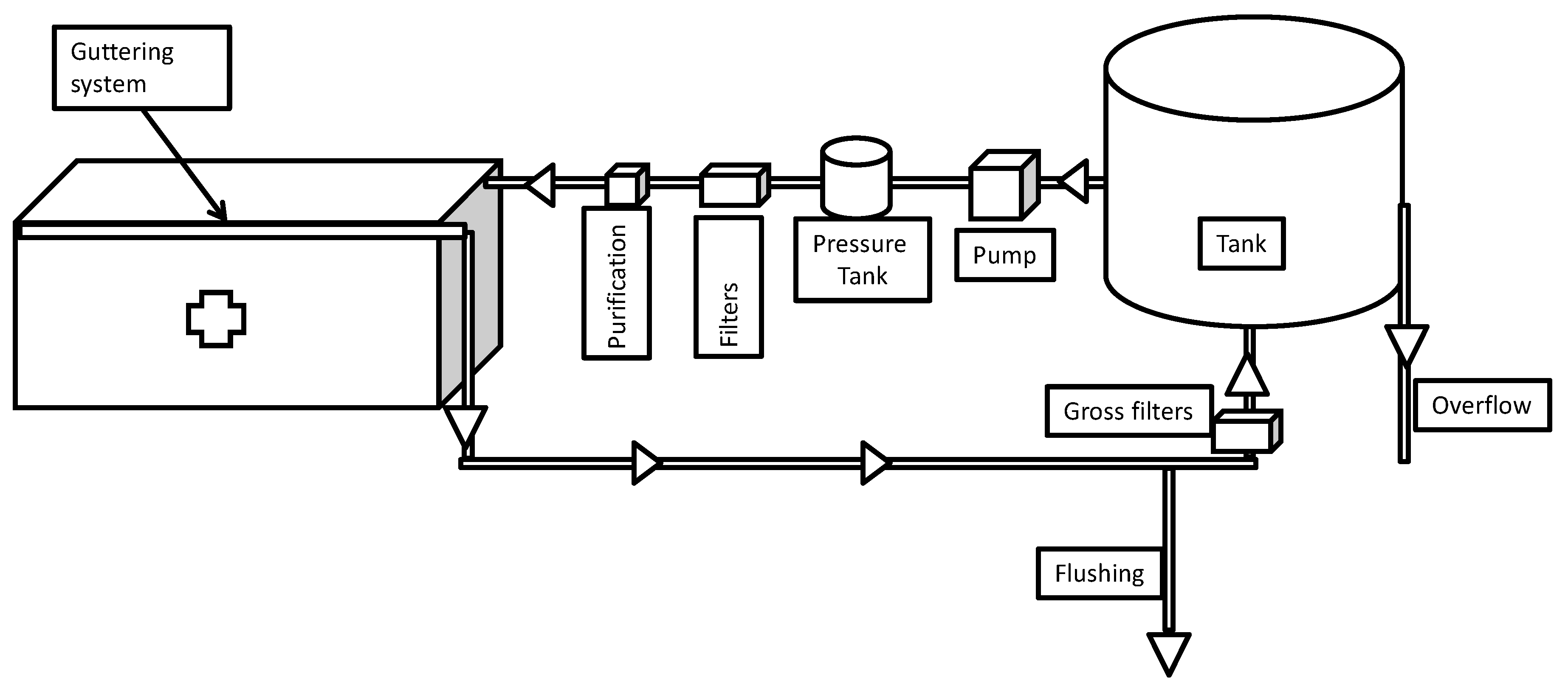
This study requires some familiarity with RWH systems, as the primary DOE components derive from that knowledge. Figure 1 is a diagram of a typical, commercial grade RWH system. Rainwater flows from capture spaces (e.g., roofs, garages, outbuildings) and is largely but not completely captured by guttering systems usually equipped with some sort of debris filter system such as screens. Some of the initial rainwater is flushed out of the system to eliminate contaminants that accumulate on the roof. Water then passes through filtration on the way to storage in a cistern, possibly with pre-treatment. A pump transfers water from the system to a pressure tank (possibly through additional filtration). On demand, water is transferred through filters of decreasing size and purification (e.g., ultraviolet light). Excess water is ejected out of the system, sometimes to non-potable tanks for irrigation of plants. This design is typical of RWH systems [3].
Although generating quality water is a major and clear concern of RWH systems, it is also well-researched [3,20,21]. Care must be taken to filtrate and purify (e.g., the use of filters, regenerable charcoal, and ultraviolet light); however, with proper care and maintenance, RWH systems produce high quality, potable, soft water. This study does not focus on the quality achievable from rainwater, but rather the feasible offset of external water consumption based on design characteristics of the RWH as well as conservation techniques such as low-flow plumbing installation. Quality of water is specifically delimited.
2.3. Study Setting & Data
This study’s setting is San Antonio, Texas. Although NOAA daily rainfall data are available for cities throughout the United States and substitution of that data into the provided simulation is trivial, San Antonio was selected for several distinguishing characteristics. San Antonio, Texas is located in a semi-arid region which routinely experiences droughts. The area has experienced a median annual rainfall of 30.4 inches over the past 71 years with significant variability year to year. Further, the population growth in the area has been robust. The increase is estimated at 12.4% from 1 April 2010 through 1 July2016, and the total population estimate is now 1.49 million [22]. These factors make the selected location ideal for evaluation, as the need to conserve water is paramount.
Supply (rainfall) data for the study were available from the NOAA [18], and the closest reporting station (San Antonio International Airport) served as the source for daily rainfall information. Daily rainfall from 1 January 1947 through 31 December 2017 provided the supply stream, as complete yearly records were available only beginning in 1947. These data are freely available from the EIA’s CBECS Study [1].
The historical data provided baseline runs to assist in validating the simulation distributions; however, the uncertain nature of rainfall suggested that alternative supply generators should be investigated [6,7]. If area rainfall trends upward or downward over time (perhaps, due to changes in climatology), then using only historical data as the supply source would not be representative of the future. Further, the effects of volatility required the evaluation of stochastic rainfall generators. For these reasons, simulations from time series models served as a secondary source of rainfall generation. Still, the historical model provided a good basis for initial investigation for this simulation which is now explicated.
2.4. Simulation: Parameters, Variables, & Flowchart
The simulation begins with the initialization of Design of Experiments (DOE) parameters (Supplementary material—“DOE”). For clarity, variables will be italicized, but parameters will be in regular type. Building size, tank holding capacity, roof capture area, and demand are important characteristics to evaluate when considering RWH systems [7,15]. Table 1 provides the operational definition of these parameters along with the source and values investigated.
The building size (BUILD) parameter is necessary to estimate the total daily demand of a hospital facility. For this simulation, some proportion of available square footage is used by a facility for capture of rainfall. Six specific building sizes are investigated ranging uniformly between 200,000 and 1.2 million square feet. The ROOF parameter (discussed below) makes that conversion.
The mean daily water demand (DEMAND) parameter is based on the building size. The Commercial Building Energy Consumption Survey (CBECS) from the US Energy Information Administration reports an average of 0.19 gallons per square foot per day are consumed by larger facilities [1]; however, we investigate the effect of demand reductions over a wide range. Just the addition of low-flow plumbing may reduce hospital consumption as much as 30% [23]. With xeriscaping and the addition of low-flow devices, it is not unreasonable to expect a 50% reduction in water consumption.
The capture area (ROOF) is based on the building size as well and is defined as the percentage of the building area (BUILD) actually used for rainwater harvesting. The capture area (ROOF) may include large, enclosed garages, outbuildings, and any area which has an appropriate roof structure and surface (either when built or after construction) that is not estimated as part of the hospital’s building space, so values above 100% are feasible, particularly if the hospital is designed in advance with rainwater harvesting in mind. Further, free-standing collection areas might also be incorporated. It is impossible to translate building square footage into capture square footage, which is why various values of ROOF capture proportions are investigated, {50%, 100%, 150%, 200%}.
The holding tank capacity (CAP) for large hospitals may include water-tower like structures, as installed in the Miami Veteran’s Hospital [24], or multiple smaller above or below-ground cisterns. The capacity of this tank is an engineering consideration that must be planned during the design/re-design phase. For this simulation, the values of {500 K gallons, 1 M gallons, 1.5 M gallons, and 2 M gallons} are investigated.
For the simulation models, the balance equation details the primary variables of interest. This model is shown as Equation (1).
Here, Vt is the volume in the tank at time t measured in gallons. C is the “capture” or rainfall supply while D is the associated demand. O is the overflow. The volume at time t must be positive, semi-definite and is restricted as such by using the maximum operator. Not shown here is that capture of water is imperfect. The Texas Manual on Rainwater Harvesting [3] suggests that capture efficiency (which is identified as E) is somewhere between 0.75 and 0.90. The simulation therefore uses a uniform distribution to model Equation (2), where St is the rainfall supply at time t. Inserting Equation (2) into Equation (1) results in a modified balance equation shown in Equation (3).
The daily rainfall in inches, St, is based on 71-years of daily NOAA data. In the historical runs (Supplementary material—“historical run”), the simulation assumes that the past rainfall data will be representative of the future. Because of potential non-stationarity (i.e., trending) and volatility of daily rainfall possibly due to changes in climatology, using a fixed, historical data stream might not represent what is achievable when adopting rainwater harvesting systems. For this reason, simulation from time series models were also investigated to model S. These time series simulations will be discussed later.
Mean values for the water demanded variable, D, derived from CBECS [1] based on average demand per square foot (DEMAND) multiplied by the total hospital square footage (BUILD). CBECS reported standard errors associated with these estimates, and these were used as part of a stochastic process. The water demanded (D) was then assumed to be from a Poisson process and modeled as an exponential distribution with a mean of 1/(DEMAND × BUILD). Because of the daily variability of demand and its strict truncation at zero, the exponential was a reasonable choice.
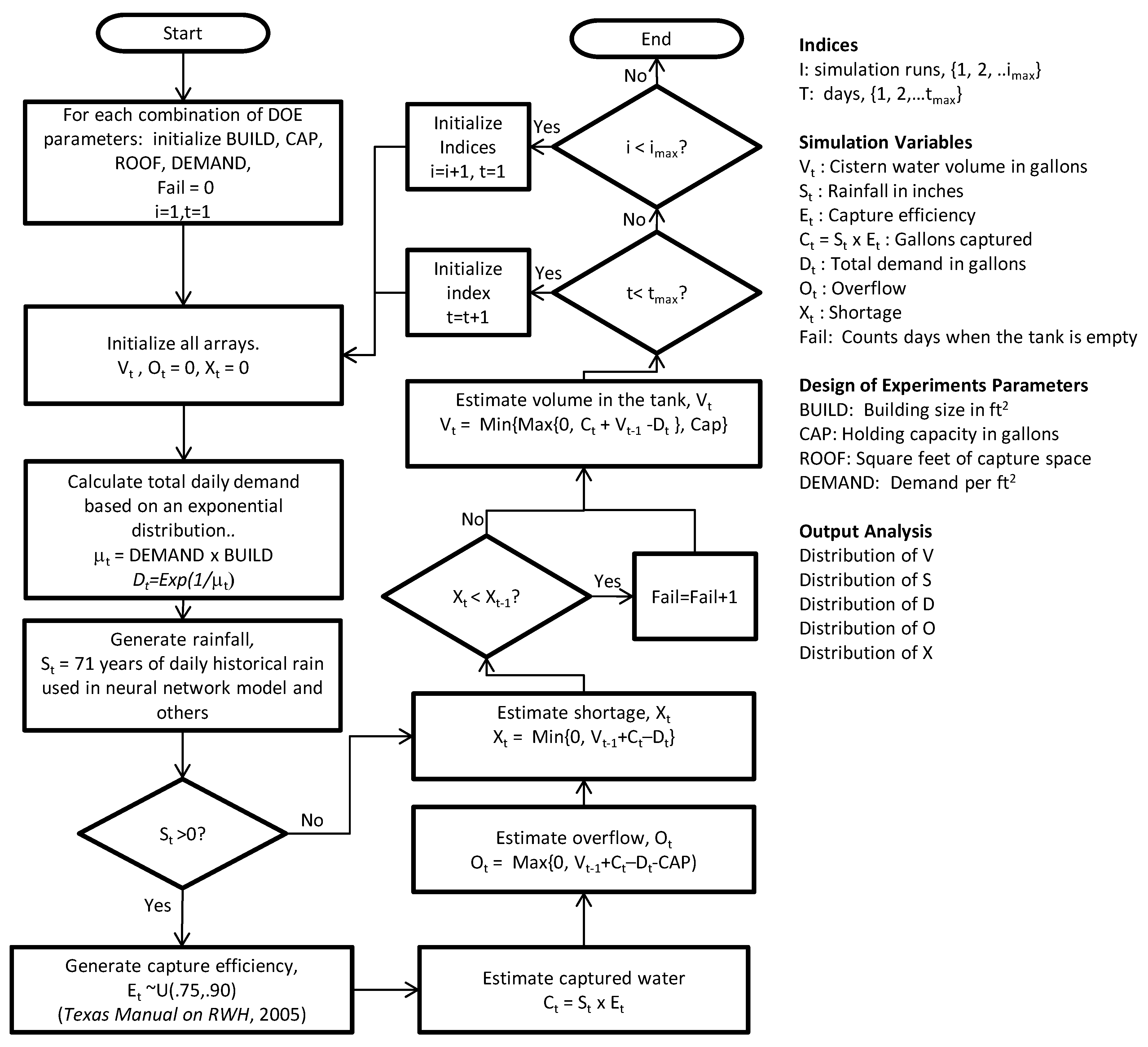
Equation (4) details all stochastic and deterministic elements associated with the simulation. Table 2 provides a complete list of variables and the associated explanations. Figure 2 depicts the variables and parameters for each iteration of the simulation model in a flowchart.
An important statistic for this simulation model was the proportion of external water demand offset that a specific design would have. Thus, the number of simulation iterations was set to ensure that the volume in the tank estimate was bracketed within 5000 gallons (margin of error, MOE), which represents 1% of the smallest tank size, a small error. The maximum standard error for volume (V) across all DOE scenarios was 4148 gl after a 25,915-day (71-years) run (excludes 29 February). Using this standard deviation, the MOE of 5000 gallons and α = 0.05, the estimate for the number of runs was calculated to be 3 as shown in Equation (5), where Z is the value for the standard normal distribution at the specified α.
With 6 building sizes (BUILD), 4 capture proportions (ROOF), 4 holding tank capacities (CAP), 3 demand parameters (DEMAND), 365 days per year, 71 years, and 3 iterations (sequence i), the total number of individual daily observations was 6 × 42 × 3 × 365 × 71 × 3 = 22,390,560 observations per rainfall generator.
2.5. Verification & Validation
To investigate validity, prior distributions were compared statistically and visually with posterior distributions. No significant differences were found. Posterior parameter values all matched the fixed values previously assigned, while the stochastic variables D (total daily demand) and E (efficiency of water capture) derived from the requisite distributions. The simulation was designed in R Statistical Software [25] using verbose commenting for debugging and the simulation flowchart (designed a priori) to reduce error. Random number seeds were used to ensure that differences in DOE replications were due to engineering design and not the selection of pseudo-random numbers. The results of the simulation runs were spot checked against direct calculations with no variability.
3. Results
3.1. Descriptive Statistics
Table 3 shows the descriptive statistics for the rainfall in the geographic region of interest. The average daily rainfall for all days in the dataset was 0.084. For only those days where rain occurred, the rainfall estimate was 0.380. Overall, 22.2% of the days experienced rainfall, although much of that was trace. As depicted previously, rainfall is seasonal.
Consumption data from CBECS [1] suggests that large hospitals, on average, consume 67.7 gallons of water per square foot per year. That statistic changes by Census region; however, consumption can range from 55.1 gl/ft2 in the Northeast to 76.0 gl/ft2 in the Midwest. There were 3040 facilities from which these statistics were derived.
Time series evaluation of rainfall is necessary to investigate any possible trends, which would change the historical analysis as well as seasonal and other components that might affect future rainfall. An analysis of the rainfall time series suggested that annual rainfall was relatively but not perfectly stationary year over year with monthly seasonality present. Figure 3 provides a yearly aggregated time series plot (beginning on 1 January 1947) with linear and loess curves superimposed. While a slight upward trend might be inferred from the linear fit, the loess curve suggests otherwise. There is no evidence of significant changes in this reporting station’s annual rainfall, although there may be multi-year periodicity associated with natural or human-made processes. As such, investigating stochastic rainfall generators as an alternative method for generating rainfall would be prudent.
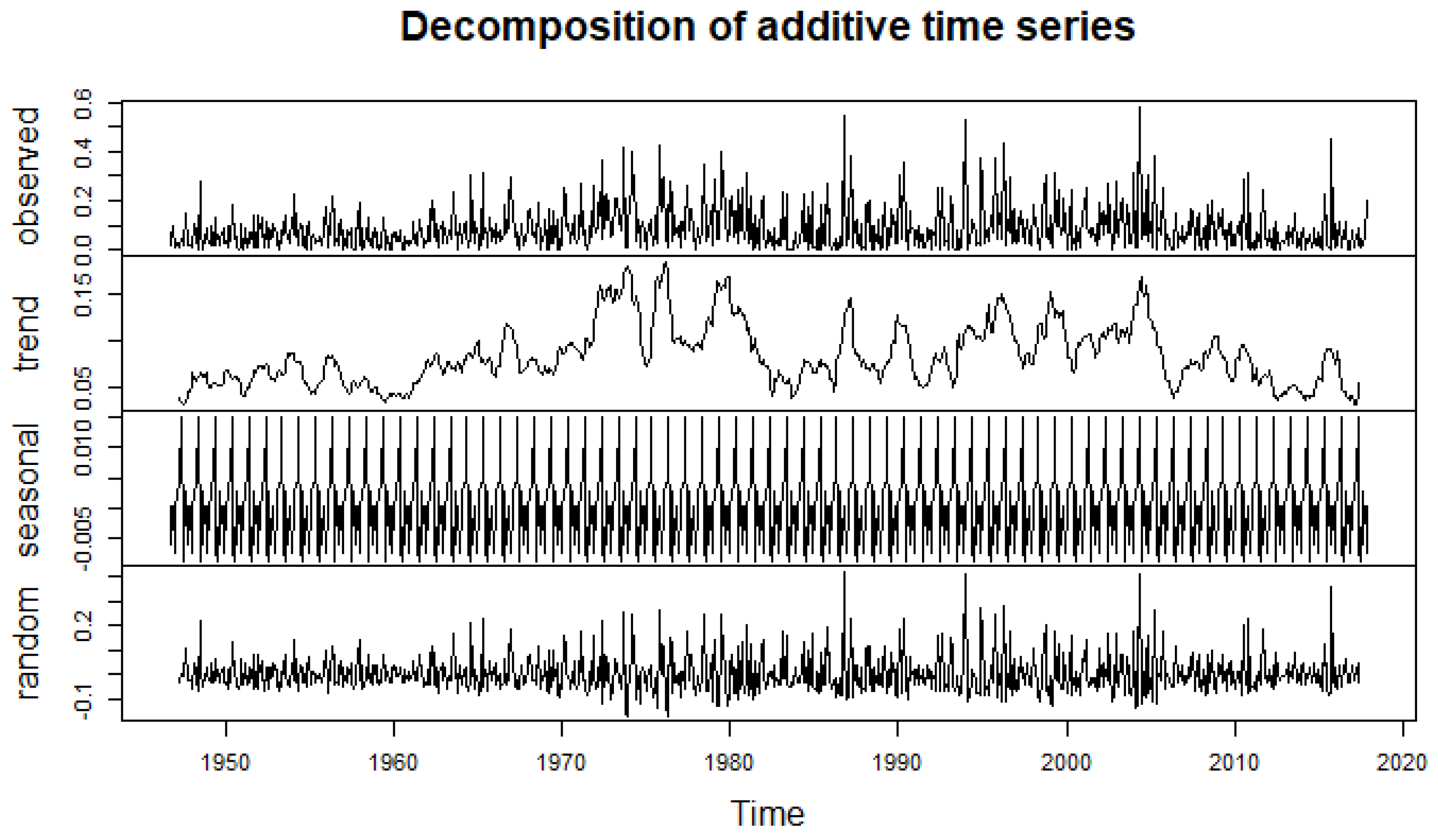
Decomposition of the monthly aggregated time series also suggest the absence of trend; however, volatility and seasonality appeared to be present. The volatility is evidenced by reviewing the error (random) components, while the seasonal components are graphed separately. Some cyclicity appears to exist, as there are multi-year waves, which are particularly noticeable starting in 1970 and extending through the mid 2000’s. Figure 4 depicts that decomposition.
Figure 5 depicts side-by-side notched boxplots by month illustrated that seasonality. Notches which do not overlap indicate statistical significance (). Darker boxplots highlight the months with the heaviest rainfall. May, June, September, and October are the months with the most significant median rainfall.
When looking at the daily time series, the volatility is clear. While aggregated data illustrate a lack of trend (yearly data) and definite seasonality (monthly data), the daily data illustrate the volatility and suggest a need to investigate rainfall generators that are stochastic. Figure 6 depicts the daily rainfall time plot.
3.2. Simulation Results, Historical Data
The results of the simulation using historical data demonstrate the offset available for various choices of the DOE parameters. The primary variable of interest was the ratio of SUPPLY/DEMAND, the proportion of the demanded water actually supplied by RWH. A second variable of interest was the proportion of time the tank was empty. If the tank was not empty on a given day, it was capable of supplying the hospital with 100% of its demand. Thus, manipulation of DOE parameters would provide engineers and designers information regarding what is necessary to offset water demand.
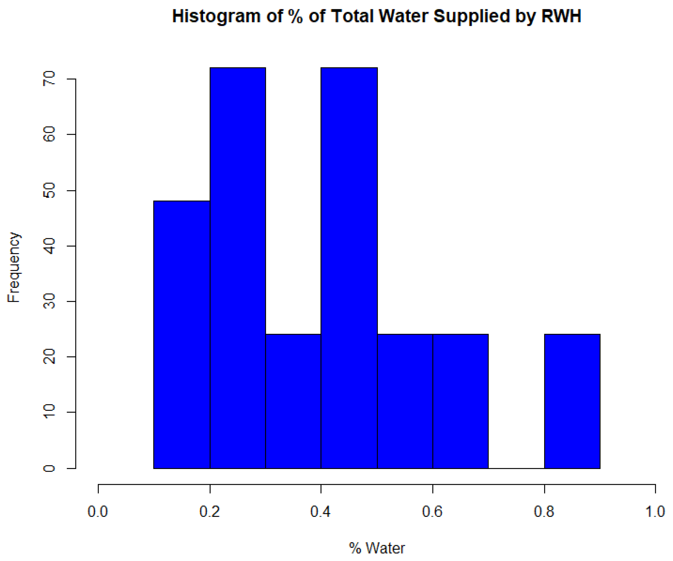
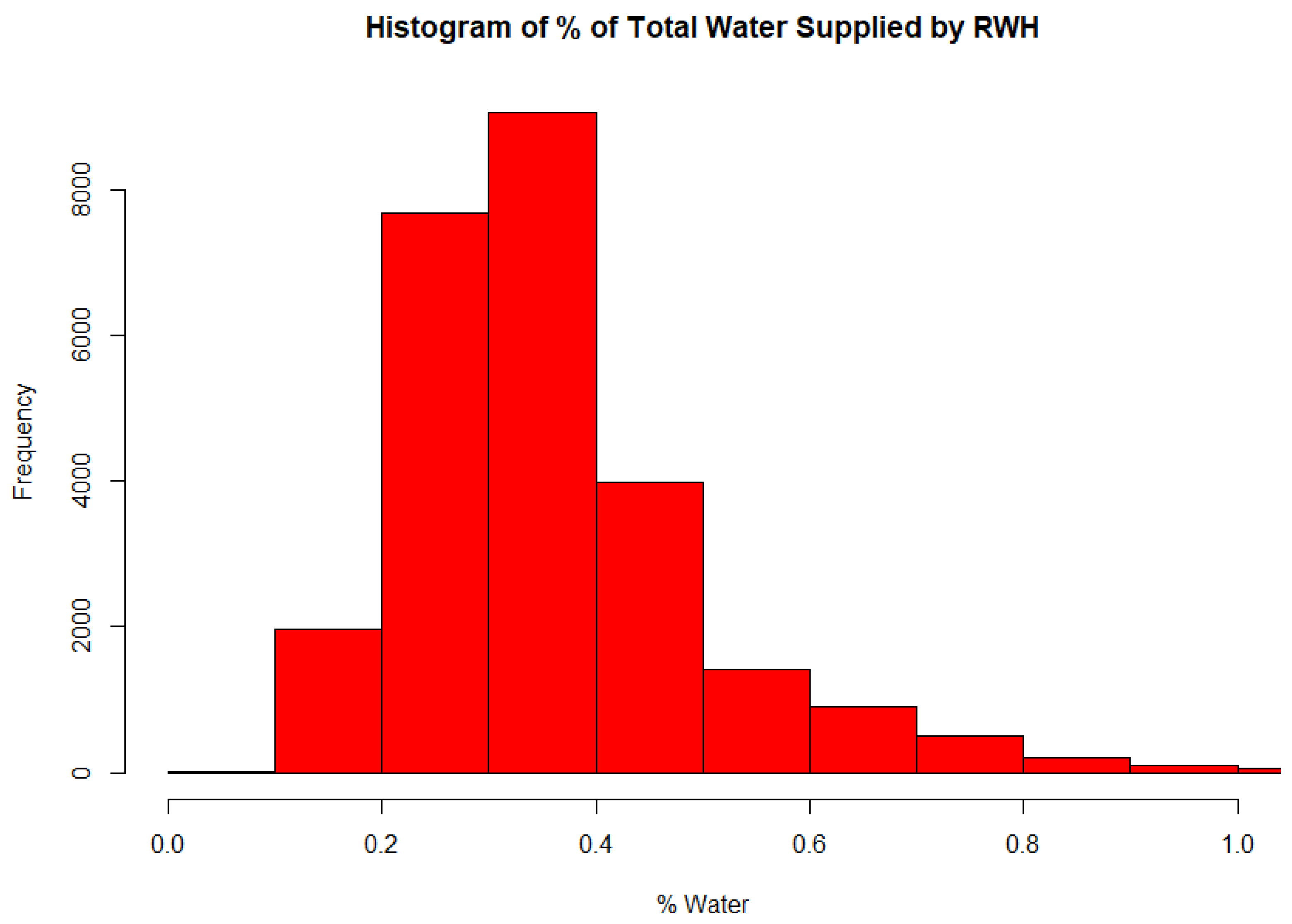
The contribution of RWH is clear from looking at the histogram of SUPPLY/DEMAND for all DOE runs. At best, RWH could eliminate 90% of the ground water and surface water demand for hospitals, reducing the impact on the environment in terms of both water and electricity. Even with the most unfavorable assumptions and design factors, a 10% reduction might be achieved. Figure 7 shows the histogram over all DOE parameters. The distribution appears bi-modal given the parameters investigated (0.2 and 0.4).
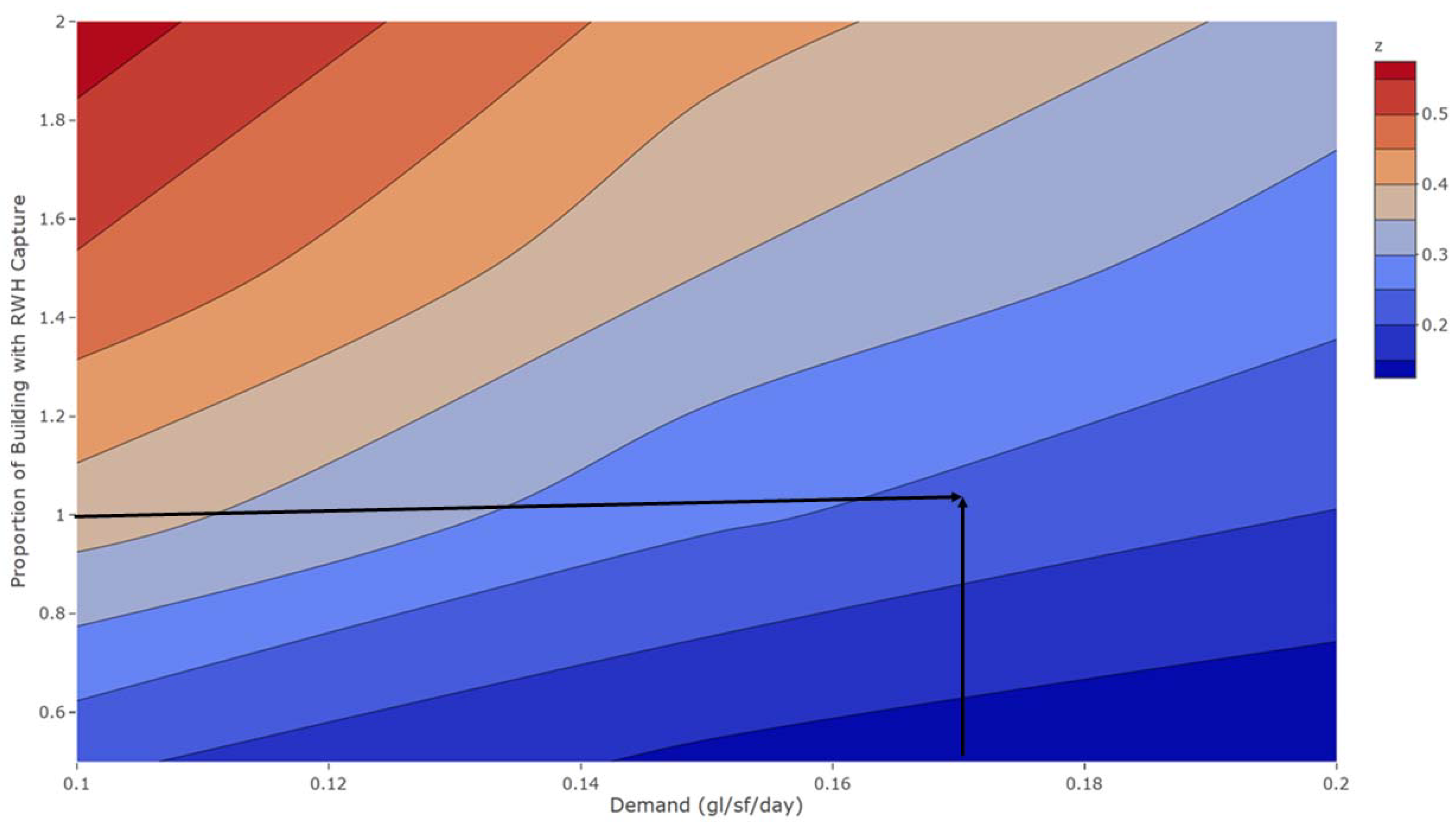
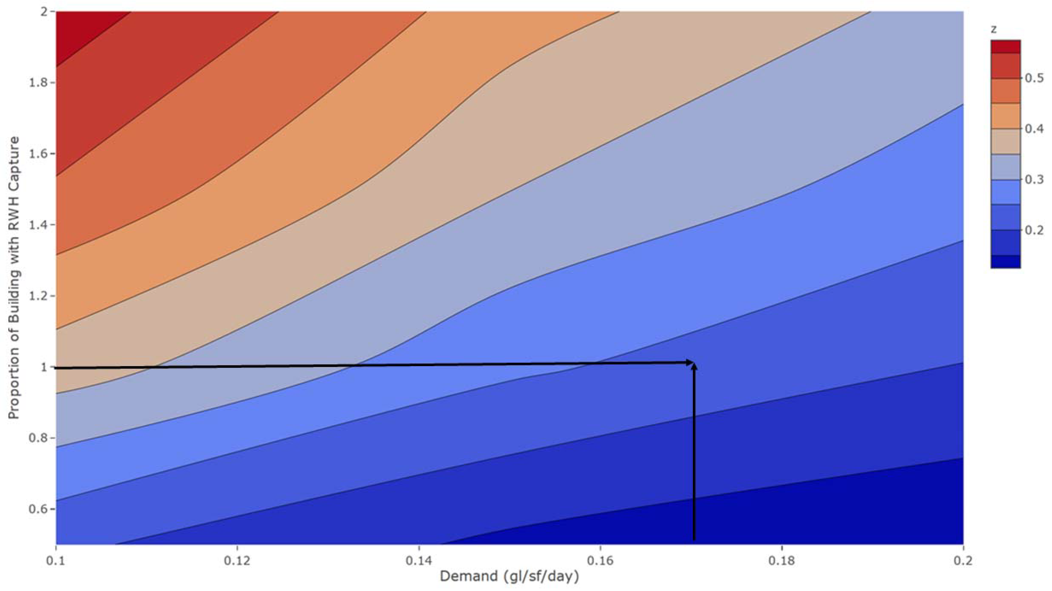
Figure 8 maps the “reliability” proportion, the proportion of days the water in the tank was not empty. This graphic depicts averages over all other DOE factor levels. What is interesting here is that using reasonable demand reductions of 10% (i.e., 0.17 gallons per square foot per day, represented by the vertical arrow on Figure 3) and adoption of rainwater harvesting at 100% (represented by the horizontal arrow on Figure 3) of built design would result in approximately 23% total reduction as depicted by the arrows in Figure 8.
Spearman’s correlation among the design parameters and the proportion of rainwater provided by RWH is shown in Table 4. The non-empty proportion was highly and positively correlated with the roof capture proportion (ρ = 0.778), while increases in demand had a predictably negative effect (ρ = −0.501). Surprisingly, the tank size had the smallest effect, although it was statistically significant at a < 0.01.
A simple multiple regression equation using only parameter terms, their squares, and the two-way interactions accounted for 99% of the variability in the average proportion of external water required using the historical data, . The value of converting the terms in the model to an equation is that this equation might be used to estimate external water reliance for this semi-arid region and the standardized coefficients provide importance indicators for each of the variables. Table 5 provides the standardized coefficients and associated p-values for the historical runs. Of particular interest is that demand reduction is of primary importance in reducing reliance on external water sources.
3.3. Time Series Models
Options for rainfall generators outside of historical data were investigated for use in a second simulation. The intent was to provide a secondary data stream to account for any variations in trend and volatility as well as the stochastic nature of rainfall. Historical data may not be fully representative of future rainfall just as historical portfolio returns may not reflect future returns. All models were built on a sequential 70% training set using the 71-years of historical data and evaluated against the remaining 30% test set (sequential). Naïve, seasonal naïve, Error, Trend & Seasonality (ETS), Auto-Regressive Integrated Moving Average (ARIMA), and a two-stage Gamma Hurdle were considered along with two stochastic, non-parametric generators and a Time Series with Neural Networks model. Each model is discussed and compared in the next sections.
The primary accuracy metrics reported here include the Mean Error (ME), the Mean Absolute Error (MAE), the Root Mean Square Error (RMSE), and the Mean Absolute Scaled Error (MASE). The ME is a measure of bias that averages the differences of the forecast values (F) from the observed values (X) for all available time period forecasts (index t), Equation (6). Ideally, time series models should identify unbiased forecasts (ME = 0).
The MAE is the average absolute difference between the observed (X) and forecast (F) scores for all available time period forecasts (index t) and is good measure of variability (Equation (7)). By taking the L1 norm, the deviations between observed and forecasts are made positive, and the MAE may be read in the original units (inches of rain).
The RMSE is the square root of the average squared difference between the observed (X) and forecast (F) scores and is a measure of variance that heavily penalizes outliers Equation (8). The squared differences are averaged and returned to their original units (e.g., inches of rain) by using the square root function.
The MASE provides a ratio of the average absolute error of the forecasting method divided by the average absolute error of the one-step naïve forecast (Equation (1)). In Equation (9), the numerator represents the Mean Absolute Error (MAE) of a forecast, while the denominator is the MAE of the naïve forecast. Ratios less than one indicate a forecasting model better than what would be expected from the naïve. The beauty of this equation is that models are evaluated against a baseline (the naïve).
3.4. Naïve Model
A naïve forecasting model is nothing more than “last = next.” The forecast for rain (F) at time t is nothing more than the observed rainfall (X) time period t − 1 (Equation (10)). The last time-period observation is used to forecast the next period, where multiple period forecasts are simply a straight-line estimate. This model provides a baseline for comparison via the Mean Absolute Scaled Error.
3.5. ETS Model
An ETS model evaluates a seasonal time series as a function of three components: smoothed error, smoothed trend, smoothed seasonality. When only the error is smoothed, ETS returns a Simple Exponential Smoothing (SES) model, where a linear combination generated by the scalar α applied to the immediately prior forecast (Ft) and the previous observation (Xt) generate the forecast. An additive version of this model is Equation (11). The scalar α is chosen through minimization of the RMSE or another variance metric.
Holt’s Trend Smoothing models may include both the SES but always have a trend smoothing component, β. Equation (12) illustrates the additive Holt’s model for a one-step forecast.
Holt and Winter’s Smoothing (or just Winter’s) include smoothed seasonality. Since the rainfall data are annual, there is no reason to believe that the previous year’s daily rainfall would have an influence on the current year’s rainfall. Since this study leverages auto-optimization of ETS, the parameters to be selected were allowed to be selected by the software, so for completeness, the formulation of the additive Holt and Winter’s model for daily data is show in Equation (13), where st is the rainfall experienced 365 days prior to the forecast and γ is the smoothing constant for the season.
To evaluate ETS models, auto-optimization of parameter coefficients was conducted using the “forecasting” library in R Statistical Software (The R Foundation for Statistical Computing, Institute for Statistics and Mathematics, Vienna, Austria) [26]. The suggested optimal parameters resulted in a simple, relatively unbiased (ME = 0.003), additive, simple exponential smoothing model: ETS(ANN), Equation (10). The RMSE of 0.324 was lower than the naïve model. and the auto-optimized model also performed just marginally better in comparison to the naïve (MASE = 0.971).
3.6. ARIMA Model
An auto-optimized Auto-Regressive, Integrated, Moving Average (ARIMA) model [26] with investigation of seasonal components was unable to provide reasonable forecasts for daily rainfall when compared to a naïve model. An ARIMA model uses autoregressors, integrated (differenced) values, and moving averages and may include these components with or without seasonality and drift. Equation (14) illustrates a non-seasonal ARIMA model on an already differenced time series vector, X′. In this equation, c represents the drift constant, the are the parameter estimates for the autoregressive terms for the differenced data, and the θ are the coefficient estimates for the moving averages. The “auto.arima()” function in R suggested an unbiased ARIMA(1,1,0) with drift but no seasonal components, yet the model was slightly biased (ME = 0.008), had higher variability than the ETS (RMSE = 0.331, MAE = 0.165), and performed worse in comparison to the naïve (MASE = 1.080).
3.7. Gamma Hurdle Model
A zero-inflated Gamma hurdle model was explored (Equation (15)). The Gamma Hurdle model uses logistic regression to evaluate the condition of rain or no rain. Given that the probability of rain is greater than 0.5 from this model, the amount of rain conditioned on the fact that it rained is modeled using a general linear model with a gamma link function. Unfortunately, this two-stage model had poor predictive accuracy when compared with the naïve model (MASE = 1.255), was slightly biased (ME = −0.056), and had a relatively high MAE (0.192).
3.8. Stochastic Rainfall Generator
In line with the work of Fulton et al. [7] and Bassinger et al. [6], a stochastic non-parametric rainfall generator was investigated to see if it might be reasonable enough to mimic the historical data stream reasonably while retaining variability. The probability of rain for any individual calendar day (365 days excluding 29 February) was estimated as a Bernoulli trial based on the empirical proportion of days rain occurred based on the 71 years of historical daily data (Supplementary material—“rain2”). The amount of rain for non-zero amounts was then estimated using the empirical distribution seen on that given day. This method of generating rain produced a slightly biased estimator (ME = 0.003) with a MAE of 0.164 and a high RMSE of 0.521 inches. The model did not perform better than the naïve (MASE = 1.072 on the test set).
3.9. Updated Stochastic, Non-Parametric Rainfall Generator
In the previous model, centered moving averages were used to estimate rainfall on the 30% test set. With 71 years of daily data, value might exist in modeling the probability of rain and the distribution of the amount of rain without averaging over 30 days. This model sampled from the marginal probability of rain by day. Given that a day received rain, the distribution of rainfall amount for that day was sampled. The results were slightly improved from the original stochastic generator but were still worse than the naïve model (MASE = 1.033).
3.10. Neural Network (NNETAR) Model
A final model for predicting model was built using time series components as well as a neural network. The model was implemented using Hyndman’s “nnetar” package in R [26]. After some parameter tuning on the training set, the model that emerged was a 5-lag, model with 1 layer consisting of 12 hidden nodes, and two external regressors (Month and Day). The slightly biased results (ME = 0.007) were impressive in terms of MAE (0.135) and MASE (0.809). This model outperformed all other models on the MAE and MASE metrics. Since the RMSE penalizes outliers (which exist in the dataset) much more heavily than the MAE, these were considered the most important statistics in evaluating a potential generator. For this reason, the neural network model served to generate forecast for our simulation. Table 6 provides the models’ performance.
3.11. Simulation Results, Time Series with Neural Net
The TS with Neural Net model served to produce estimates for rainfall in the second simulation, as it proved to be reasonable for forecasting an unseen test set. When applied to the entire dataset, the model was unbiased (ME = 0) with an RMSE of 0.34 and an MASE of 0.836. These values were superior to other TS models considered on the full data set. Using this rainwater stream, the results for the simulation were similar yet not identical to the historical data.
Evaluating the histogram of SUPPLY/DEMAND for all DOE runs using the neural network distribution (Figure 9) illustrates that, depending on parameters, offsets near 100% might be achievable depending on build and demand assumptions. The distribution is not identical to that of the historical data (unimodal, skewed right), as error in forecasting is somewhat smoothed. The modal range appears to be about 0.30 given the parameter values investigated. This is congruent with the average of the bimodal values (2 and 0.4) from the historical data.
Figure 10 maps the “reliability” proportion, the proportion of days the water in the tank was not empty for the TS with Neural Net model. This graphic depicts averages over all other DOE factor levels. What is interesting here is that using reasonable demand reductions of 10% (i.e., 0.17 gallons per square foot per day, represented by the vertical arrow on Figure 3) and adoption of rainwater harvesting at 100% (represented by the horizontal arrow on Figure 3) of built design would result in approximately 24% total reduction as depicted by the arrows in Figure 10. While the isobars are certainly not identical to the historical model, the neural net time series appears to be congruent with the historical model. This suggests that either historical or forecast data would work well for estimating requirements.
4. Discussion
In this study, demand and supply-side measures were investigated for their effects on reducing water consumption among the group of large commercial buildings consuming the highest quantity of this resource: large hospitals. While the study focused on a single semi-arid region, the methods are generalizable outside of this region.
Part of the analysis required some exploration of rainwater time series. For the region under investigation, no trend was observed; however, seasonality and volatility existed. After exploration of several methods, a neural network rainfall generator was selected along with the use of historical data.
The results of the simulation demonstrated achievable deductions of external water usage in the 20–30% range without much adjustment of demand behavior. Given the high water-usage of large hospitals, this savings might represent 18 to 27 million gallons saved per year. Further, the use of RWH is more efficient than using groundwater, as the efficiency of system capture is 75–90% versus standard absorption. RWH reduces runoff and non-point source pollution [3], and RWH also reduces energy demands for water transport. The associated savings in kWh requires additional investigation; however, states like California which spend 30% on moving and treating water would expect significant reductions in kWh energy usage.
Based on Spearman’s correlation, the proportion of building square footage used for rainwater capture is the most important metric followed by the reduction in demand through the adoption of low-flow plumbing, xeriscaping, and other conservation measures proxied as demand reduction. For new facilities, rainwater capture, xeriscaping, and low-flow devices should be considered as part of the design process. Retrofitting older facilities with RWH may be more challenging depending on the design characteristics, but, the socially responsible solution is to reduce demand and increase internal collection via harvesting where possible. Even without an RWH, reduction in demand should be a sustainability priority in all hospitals, particularly in semi-arid regions. The culture of the organization must support sustainability, though, and this may be the hardest problem to address.
This analysis is specifically designed for semi-arid regions, and while the rainfall was selected for a single region, it is trivial to replace this stream for evaluation of other areas. The intent of the paper is to highlight what might be achieved in difficult regions. For regions which experience more rain, the offset in water and electricity would be even more impressive.
As stewards of human health, hospitals have a responsibility to be conservators of resources as well. The two cannot be considered separately. The developed environment requires custodial care to support us, and the inclusion of smart designs for hospitals is important.
Supplementary Materials
The following are available online at https://0-www-mdpi-com.brum.beds.ac.uk/2071-1050/10/5/1659/s1.
Conflicts of Interest
The author declares no conflict of interest.
References
- U.S. Energy Information Administration. Available online: https://www.eia.gov/consumption/commercial/reports/2012/water/ (accessed on 18 March 2018).
- Texas Commission on Environmental Quality. Available online: https://www.tceq.texas.gov/drinkingwater/trot/location.html (accessed on 18 March 2018).
- Texas Water Development Board. Available online: http://www.twdb.texas.gov/publications /brochures/conservation/doc/RainwaterHarvestingManual_3rdedition.pdf (accessed on 18 March 2018).
- Abdulla, F.A.; Al-Shareef, A.W. Roof rainwater harvesting systems for household water supply in Jordan. Desalinization 2009, 243, 195–207. [Google Scholar] [CrossRef]
- Jones, M.P.; Hunt, W.F. Performance of rainwater harvesting systems in the southeastern United States. Resour. Conserv. Recycl. 2010, 54, 623–629. [Google Scholar] [CrossRef]
- Basinger, M.; Montalto, F.; Lall, U. A rainwater harvesting system reliability model based on nonparametric stochastic rainfall generator. J. Hydrol. 2010, 392, 105–118. [Google Scholar] [CrossRef]
- Fulton, L.V.; Bastian, N.D.; Mendez, F.A.; Musal, R.M. Rainwater harvesting system using a non-parametric stochastic rainfall generator. Simulation 2012, 89, 693–702. [Google Scholar] [CrossRef]
- Guo, Y.; Baetz, B.W. Sizing of rainwater storage units for green building applications. J. Hydrol. Eng. 2007, 12, 197–205. [Google Scholar] [CrossRef]
- Lall, U.; Sharma, A. A nearest neighbor bootstrap for resampling hydrologic time series. Water Resour. Res. 1996, 32, 679–693. [Google Scholar] [CrossRef]
- Al-Houri, Z.; Abu-Hadba, O.; Hamdan, K. The potential of roof top rain water harvesting as a water resource in Jordan: Featuring two application case studies. Int. J. Environ. Chem. Ecol. Geol. Geophys. Eng. 2014, 8, 147–153. [Google Scholar]
- Domènech, L.; Saurí, D. A comparative appraisal of the use of rainwater harvesting in single and multi-family buildings of the metropolitan area of Barcelona (Spain): Social experience, drinking water savings and economic costs. J. Clean. Prod. 2011, 19, 598–608. [Google Scholar] [CrossRef]
- Ennenbach, M.; Larraui, P.; Lall, U. County-scale rainwater harvesting feasibility in the United States: Climate, collection area, density, and reuse considerations. J. Am. Water Resour. Assoc. 2018, 54, 255–274. [Google Scholar] [CrossRef]
- World Health Organization. Available online: http://www.searo.who.int/ entity/water_sanitation/topics/rainwater/en/ (accessed on 18 March 2018).
- The Hindu. Available online: http://www.thehindu.com/news/cities/Delhi/ngt-fines-malls-hospitals-hotels-over-rainwater-harvesting/article7195788.ece (accessed on 18 March 2018).
- Krishna, H. An Overview of Rainwater Harvesting Systems and Guidelines in the United States. In Proceedings of the First American Rainwater Harvesting Conference, Austin, TX, USA, 21–23 August 2003. [Google Scholar]
- Klein, G.; Krebs, M.; Hall, V.; O’Brien, T.; Blevins, B. California’s Water-Energy Relationship. 2005 Integrated Energy Policy Report Proceeding. California, November 2005. Available online: http://large.stanford.edu/courses/2012/ph240/spearrin1/docs/CEC-700-2005-011-SF.PDF (accessed on 30 November 2017).
- Greater Edwards Aquifer Alliance. Available online: https://aquiferalliance.org/aquifer-at-risk/ (accessed on 18 March 2018).
- National Oceanic and Atmospheric Administration. Available online: https://www.ncdc.noaa.gov/cdo-web/datasets/LCD/stations/WBAN:12921/detail (accessed on 11 May 2018).
- Milley, P.C.D.; Betancourt, J.; Falkenmark, M.; Hirsch, R.; Kundzewicz, Z.W.; Lettenmaier, D.P.; Stouffer, R.J. Stationarity is dead: Whither water management? Sci. Mag. 2008, 319, 573–574. [Google Scholar] [CrossRef] [PubMed]
- Evans, C.A.; Coombes, P.J.; Dunstan, R.H. Wind, rain and bacteria: The effect of weather on the microbial composition of roof-harvested rainwater. Water Res. 2006, 40, 37–44. [Google Scholar] [CrossRef] [PubMed]
- Magyar, M.I.; Mitchell, V.G.; Ladson, A.R.; Diaper, C. An investigation of rainwater quality and sediment dynamics. Water Sci. Technol. 2007, 56, 21–28. [Google Scholar] [CrossRef] [PubMed]
- United States Census Bureau. Available online: https://www.census.gov/quickfacts/fact/table/sanantoniocitytexas/PST045217 (accessed on 18 March 2018).
- Durio, S. Dell Childrens’ Medical Center: Taking green building to highest level. Tex. Hosp. 2006, 3, 112–234. [Google Scholar]
- AKEA. Available online: http://www.akeainc.com/projects/design-build/item/1-million-gallon-elevated-water-storage-tank (accessed on 18 March 2018).
- R Core Team. R: A language and environment for statistical computing. R Foundations for Statistical Computing: Vienna, Austria. 2016. Available online: http://www.R_project.org/ (accessed on 18 March 2018).
- Hyndman, R. fpp: Data for “Forecasting principles & practice”. R package version 0.5. Available online: https://CRAN.R-project.org/package=fpp (accessed on 18 March 2018).
Figure 1.
An example of an RWH system.

Figure 2.
Flowchart for the simulation.

Figure 3.
Rainfall distribution by year.
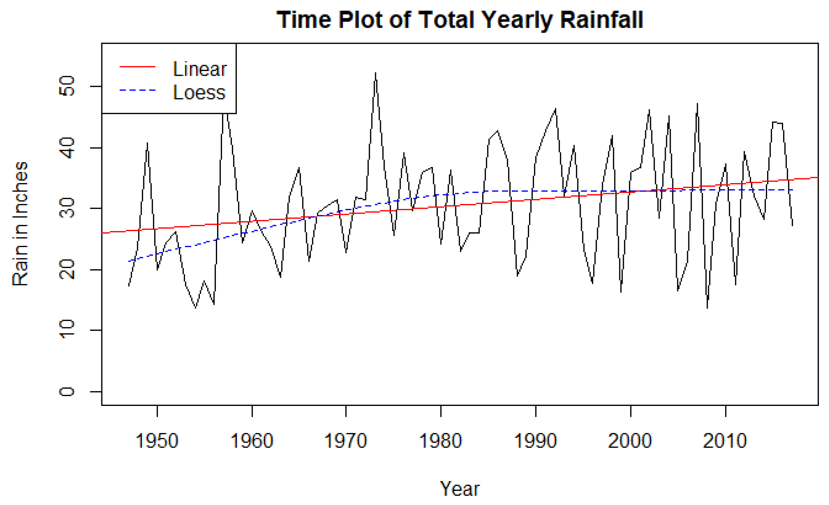
Figure 4.
Decomposition of monthly rainfall using R [25].
Figure 4.
Decomposition of monthly rainfall using R [25].

Figure 5.
Notched boxplot of mean daily rainfall.
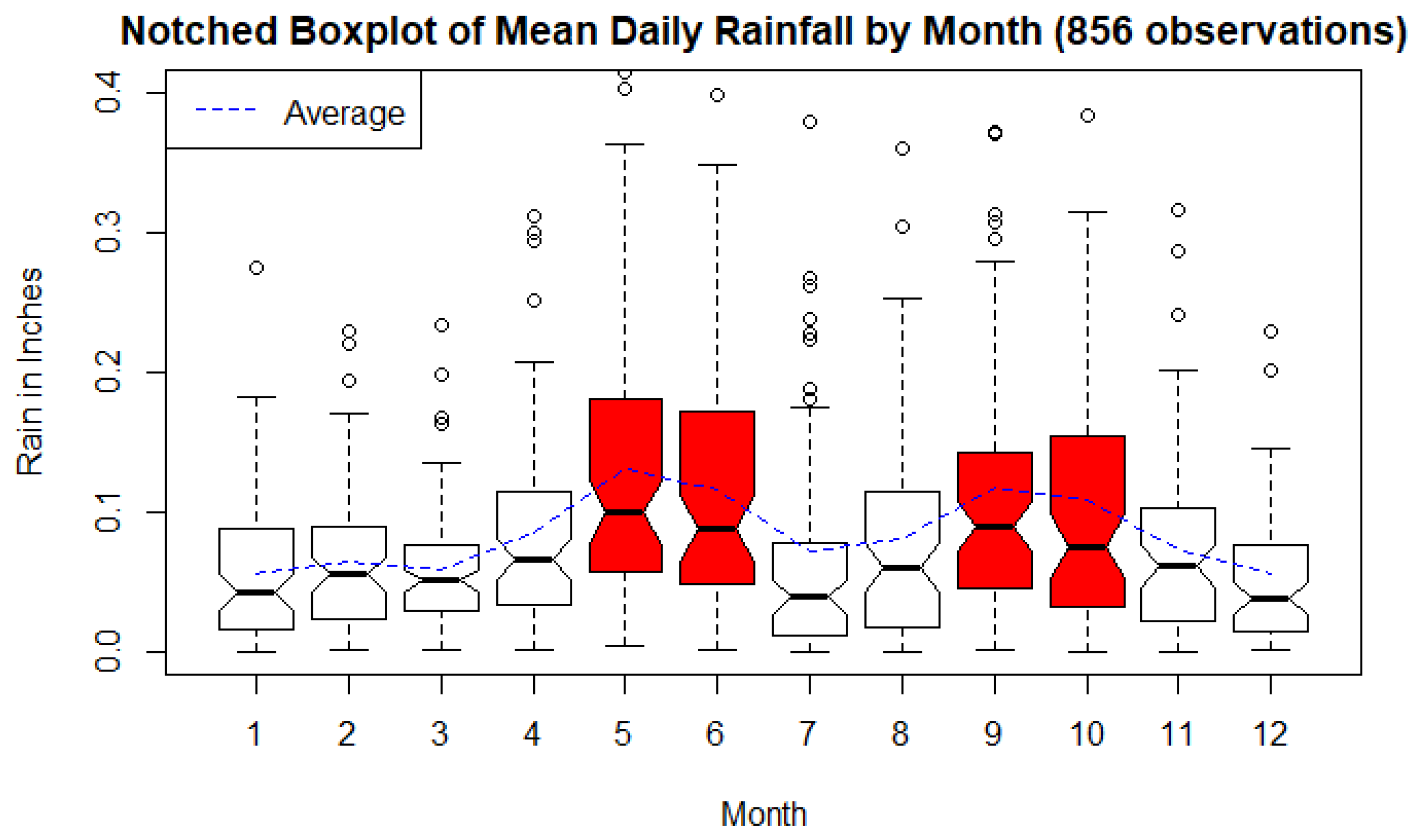
Figure 6.
Time plot of daily rainfall.
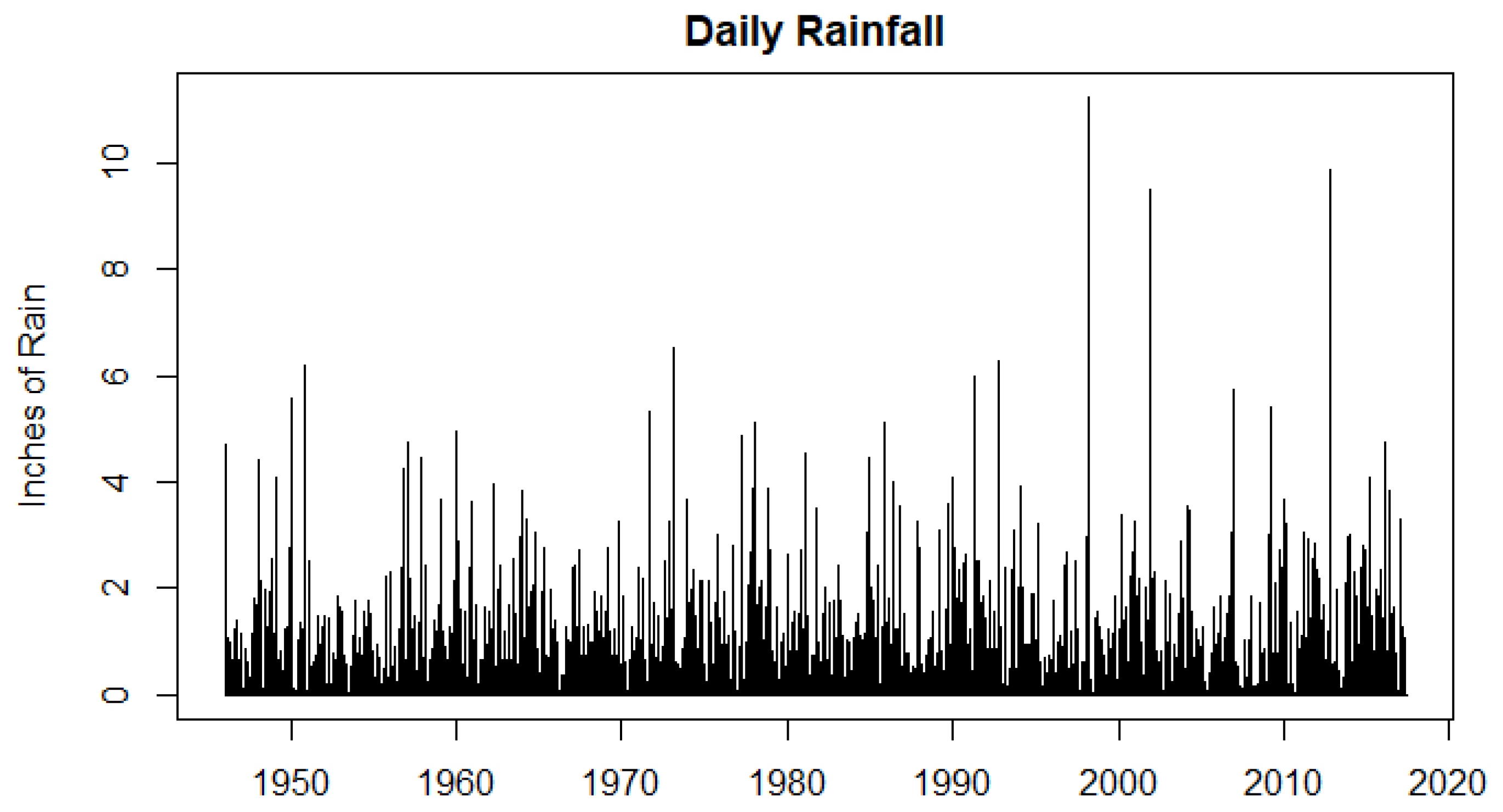
Figure 7.
Histogram of % water supplied by RWH (SUPPLY/DEMAND).

Figure 8.
This figure depicts a contour plot of the proportion of days the tank would not be empty (z-axis, the contours) versus the demand in gallons per square foot per day (x-axis) and the proportion of building size that is assigned RWH capability (e.g., 100% of the building = 1.0, (y-axis). Arrows indicate a 10% reduction in demand and square footage for rainfall capture equivalent to building size. The corresponding proportion of demand axis (contour) is roughly 0.23 (23%).

Figure 9.
Histogram demonstrating Supply/Demand for the neural network stream.

Figure 10.
This figure depicts a contour plot of the proportion of days the tank would not be empty (z-axis, the contours) versus the demand in gallons per square foot per day (x-axis) and the proportion of building size that is assigned RWH capability (e.g., 100% of the building = 1.0, (y-axis). Arrows indicate a 10% reduction in demand and square footage for rainfall capture equivalent to building size. The corresponding proportion of demand axis (contour) is approximately 0.24 (24% reduction).

Table 1.
Design of experiments parameters for the simulation.
| Parameter Name | Operational Definition | Values Investigated | Notes |
|---|---|---|---|
| BUILD | Building size, ft2 | {200 K, 400 K, 1.2 M} | Definition of Large Hospital [1] |
| DEMAND | Water demand, gl/ft2/day. | {0.10, 0.15, 0.20} | For large hospitals, CBECS [1] reports 0.19 gl/ft2/day. |
| ROOF | % building ft2 used for RWH | {50%, 100%, 200%} | |
| CAP | Holding capacity, gl | {500 K, 1 M, 1.5 M, 2 M} |
Table 2.
Variables.
| Variable Name | Operational Definition | Type | Comments |
|---|---|---|---|
| V | Volume in the tank, gl | Quantitative | Equation (1), Balance Equation |
| S | Daily rainfall, inches | Quantitative | Derived from NOAA [18] |
| E | Capture efficiency Et ~U(0.75, 0.90) | Quantitative | Texas Manual on Rainwater Harvesting [3] |
| C | Water captured, gallons | Quantitative | Equation (2) |
| D | Water demanded, gallons | Quantitative | CBECS [1] |
| O | Overflow, gallons | Quantitative | Calculated if Vt−1 + Ct − Dt > CAP |
| X | Shortage, gallons | Quantitative | Calculated if Vt−1 + Ct < Dt |
| Empty | Empty Status, Indicator | Qualitative | {0 = not empty, 1 = empty} |
Table 3.
Descriptive statistics for rainfall.
| N | Mean | SD | Median | Min | Max | |
|---|---|---|---|---|---|---|
| Daily Rainfall, All Days | 26,055 | 0.084 | 0.352 | 0.000 | 0.000 | 11.260 |
| Daily Rainfall, Rainy Days | 5781 | 0.380 | 0.669 | 0.120 | 0.010 | 11.260 |
| Proportion Rained Overall | 26,055 | 0.222 | 0.416 | 0.000 | 0.000 | 1.000 |
Table 4.
Spearman’s Correlations, All Statistically Significant at p < 0.01.
| Parameter | Building Size | Roof % | Tank Capacity | Demand/ft2 |
|---|---|---|---|---|
| % Not Empty | −0.193 | 0.778 | 0.189 | −0.501 |
Table 5.
Table of standardized regression coefficients for the DOE parameter fit.
| Parameter | β | Se | t | p |
|---|---|---|---|---|
| BUILD | −0.369 | 0.0375 | −8.587 | <0.001 |
| ROOF | 1.813 | 0.0404 | −21.605 | <0.001 |
| CAP | 0.334 | 0.0404 | 58.796 | <0.001 |
| DEMAND | −1.102 | 0.0604 | 20.218 | <0.001 |
| BUILD^2 | 0.152 | 0.0267 | 5.265 | <0.001 |
| ROOF^2 | −0.541 | 0.0309 | 11.293 | <0.001 |
| CAP^2 | −0.293 | 0.0309 | −36.202 | <0.001 |
| DEMAND^2 | 0.906 | 0.0569 | −12.662 | <0.001 |
| BUILD × ROOF | −0.460 | 0.0174 | −9.711 | <0.001 |
| BUILD × CAP | 0.129 | 0.0174 | 7.497 | <0.001 |
| BUILD × DEMAND | 0.288 | 0.0235 | 7.369 | <0.001 |
| ROOF × CAP | 0.427 | 0.0181 | −5.972 | <0.001 |
| ROOF × DEMAND | −0.639 | 0.0240 | 2.559 | <0.001 |
| CAP × DEMAND | −0.267 | 0.0240 | −3.169 | <0.001 |
Table 6.
Comparison of models on 30% test set.
| Model | ME | RMSE | MAE | MASE |
|---|---|---|---|---|
| ETS(ANN) | 0.00 | 0.32 | 0.15 | 0.97 |
| ARIMA(1,1,0) | 0.01 | 0.33 | 0.17 | 1.08 |
| Gamma Hurdle | −0.06 | 0.39 | 0.19 | 1.25 |
| Stochastic Generator 1 | 0.00 | 0.52 | 0.16 | 1.07 |
| Stochastic Generator 2 | 0.01 | 0.51 | 0.16 | 1.03 |
| TS with Neural Net | 0.01 | 0.38 | 0.14 | 0.88 |
© 2018 by the author. Licensee MDPI, Basel, Switzerland. This article is an open access article distributed under the terms and conditions of the Creative Commons Attribution (CC BY) license (http://creativecommons.org/licenses/by/4.0/).
Share and Cite
MDPI and ACS Style
Fulton, L.V. A Simulation of Rainwater Harvesting Design and Demand-Side Controls for Large Hospitals. Sustainability 2018, 10, 1659. https://0-doi-org.brum.beds.ac.uk/10.3390/su10051659
AMA Style
Fulton LV. A Simulation of Rainwater Harvesting Design and Demand-Side Controls for Large Hospitals. Sustainability. 2018; 10(5):1659. https://0-doi-org.brum.beds.ac.uk/10.3390/su10051659
Chicago/Turabian StyleFulton, Lawrence V. 2018. "A Simulation of Rainwater Harvesting Design and Demand-Side Controls for Large Hospitals" Sustainability 10, no. 5: 1659. https://0-doi-org.brum.beds.ac.uk/10.3390/su10051659
Note that from the first issue of 2016, this journal uses article numbers instead of page numbers. See further details here.