A Location-Inventory Problem in a Closed-Loop Supply Chain with Secondary Market Consideration


1
School of Management, Jinan University, Guangzhou 510632, China
2
Department of Industrial and Systems Engineering, The State University of New York at Buffalo, Buffalo, NY 14260, USA
3
Department of Accounting, Temple University, Philadelphia, PA 19122, USA
4
School of Information Management, Central China Normal University, Wuhan 430079, China
*
Authors to whom correspondence should be addressed.
Sustainability 2018, 10(6), 1891; https://0-doi-org.brum.beds.ac.uk/10.3390/su10061891
Submission received: 30 April 2018
/
Revised: 20 May 2018
/
Accepted: 1 June 2018
/
Published: 5 June 2018
(This article belongs to the Special Issue Sustainable Supply Chain System Design and Optimization)
Abstract
:To design sustainable supply chain systems in today’s business environment, this paper studies a location-inventory problem in a closed-loop supply chain by considering the sales of new and used products in the primary and secondary markets, respectively. This problem is formulated as a mixed-integer nonlinear program to optimize facility location and inventory management decisions jointly, and the logistics flows between the two markets are modeled dynamically. To solve this problem efficiently, a new heuristic approach is also developed by introducing an effective adaptive mechanism into differential evolution. Finally, numerical experiments are presented to validate the solution approach and provide valuable managerial insight. This paper makes a meaningful contribution to the literature by incorporating the secondary market into the study of closed-loop supply chains, and practically, it is also greatly beneficial to improve the sustainability and efficiency of modern supply chains.
1. Introduction
Consumer returns [1] are a common phenomenon in today’s business, and they become much more frequent as the rapid growth of e-commerce and the intense competition in the retailing industry. According to the National Retail Federation, the amounts of merchandise returned were $260.5 and $28.3 billion dollars in the U.S. and Canadian in 2015, respectively [2]. The average return rate for online products has reached 22% and it is still increasing [3], and at least 30% of all the products ordered online are returned as compared to 8.89% of that sold in traditional offline stores [4]. Particularly, for fashion products such as fashion apparel, it can be as high as 75% [5].
Consequently, considerable attention is paid to customer returns to improve the sustainability and efficiency of traditional supply chains. Closed-loop supply chains (CLSCs) [6] are an emerging concept that considers returned products in a logistics system. In a CLSC, there are reverse flows of used products (postconsumer use) back to manufacturers as well as the forward flow which is unidirectional from suppliers to manufacturers to distributors to retailers, and to consumers [7]. To further improve the sustainability of CLSCs, returned products can be disposed by considering their life cycles and the related services. In practice, secondary markets are important for retailers to sell off excess inventory and used items, and returned products can be reconditioned or refurbished [8] and then sold to secondary markets [9]. For example, automotive companies tend to provide whole life cycle service to the cars sold to their customers, and hence they can make profits from the service in early days and then from the sales of the used cars in the secondary market. In the consumer electronics industry, it is also a common practice to determine whether a product should be disposed or resold according to its life cycle. Usually, an end-of-life product will be disassembled into components or parts, but a new or fairly new product will be resold in the secondary market for more profits. Currently, many retailers have entered secondary markets to extend their business. For example, JD.com, which is one of the two largest B2C online retailers in China by transaction volume and revenue, launched a new program called “Paipai second-hand” to sell used products in secondary markets, and its main competitor, Alibaba Group, also invested in MEI.COM that sells discounted luxury products in those markets. Although secondary markets are very important and have a close relationship with CLSCs in practice, they are rarely considered in the CLSC literature. Therefore, it will be greatly beneficial to study CLSCs by incorporating secondary markets to represent the real-world business of significant interest and value.
This paper studies a joint location-inventory problem in a closed-loop supply chain by considering the secondary market. In such a system, a retailer will make three types of business decisions: (i) Choosing locations for its hybrid distribution-collection centers (HDCCs); (ii) Assigning HDCCs to customer zones in the forward and reverse flows; and (iii) Planning inventory replenishment for the primary and secondary markets. We develop a mix-integer nonlinear programming model to optimize the facility location, facility-customer assignment, and inventory replenishment decisions simultaneously, and we also design a novel self-adaptive differential evolution algorithm to solve this model efficiently. From a practical perspective, the research questions and gaps that motivate this study are summarized as follows:
- How can the logistics flows and interaction between the primary and secondary markets be formulated?
- What are the optimal facility location, facility-customer assignment, and inventory replenishment decisions in a CLSC when the primary and secondary markets are both considered?
- Which parameters are significant to the cost functions and business decisions in such a system?
The rest of this paper is organized as follows: Section 2 reviews the literature related to location-inventory problems, closed-loop supply chains, and secondary markets. Section 3 describes the research problem under study and formulates it as a mixed-integer nonlinear programming model. Section 4 proposes an improved self-adaptive differential evolution algorithm to solve the model efficiently. Section 5 presents the numerical study and computational results. Section 6 concludes this paper and provides directions for future research.
2. Literature Review
Sustainable supply chain design plays an important role in many industries, and it is greatly beneficial to pollution reduction and environmental protection. Currently, customer returns [10] are a common phenomenon in the real-world business, and they become much more frequent as the rapid growth of e-commerce. To enhance the disposal of returned products and improve the sustainability of today’s supply chains, this paper studies a location-inventory problem (LIP) in a closed-loop supply chain (CLSC) by incorporating the secondary market. Therefore, our study is related to three research streams, which are closed-loop supply chain, secondary market, and location inventory problem.
The closed-loop supply chain is an important topic of significant impact in practice because of the rising awareness of environmental issues. In the literature, CLSCs are extensively studied by incorporating many real-world businesses such as manufacturing and remanufacturing [11,12], dual recycling channels [13], environmental regulations [14], material management [15], and disruption risks [16]. They are also investigated from the perspective of supply chain coordination [17,18], and Govindan et al. [19] presents a comprehensive and thorough review on the related works. Since a main motivation to study CLSCs come from governmental legislation that forced producers to take care of their end-of-life (EOL) products, most research efforts on CLSCs are focused on the disposal of EOL products [20,21] without considering the life cycles of the products and services. However, nowadays, many returned products are in new or fairly new conditions, and they represent a large body of the reverse logistics in reality. Therefore, there will be a big gap if it is assumed that the reverse logistics in a CLSC only consists of EOL products that need to be recycled and disposed, and it is greatly beneficial to consider the whole life cycle and study how to handle the returned products in new or good conditions effectively to improve the performance and sustainability of modern supply chains.
Secondary markets have become an important marketplace for business organizations to sell off excess inventory or used products, and it is a common practice to resell returned products of good quality at a discounted price in a secondary market. Because of their great importance in practice, secondary markets have attracted much research attention in the literature [22]. For example, Angelus [23] investigates how to dispose excess inventory of new products in secondary markets, and more recent works are extended to refurbished products by considering refurbishing authorization strategy [9], product upgrade decisions [24], and consumer return policies [25]. To study the impact of secondary markets on supply chains, Lee and Whang [26] find that the secondary market creates two interdependent effects, i.e., a quantity effect regarding the sales by a manufacturer and an allocation effect that is related to supply chain performance. He and Zhang [27] also show that the secondary market will have a positive impact on supply chain performance in general. In practice, an important consideration for the sales of used products in a secondary market is their sources, and it is not unusual to see that those products come from the returned or recycled items in a CLSC. However, the interaction between CLSCs and secondary markets is rarely studied in the literature. To fill this gap, we consider such interaction dynamically in this study, and hence it can well represent the reality.
Nowadays, many business decisions are made jointly instead of separately to improve supply chain performance, and it is a common practice to integrate facility location [28], inventory management, and vehicle routing problems and solve them together. Correspondingly, the first two problems can be integrated into location-inventory problems (LIPs) [29], and all of them can be combined as location-inventory-routing problems [30]. In the literature, LIPs were first proposed by Daskin et al. [31] and Shen et al. [32], and they have been studied extensively in several directions thereafter. For example, location-inventory models are extended to consider difference inventory control strategies [33], uncertain or correlated demands [34,35], lateral transshipment [36], product attributes (e.g., perishable products, seasonal products, substitutable products, etc.) [37,38], and third-party logistics [39]. As the emergence of CLSCs, LIPs are also studied by considering reverse logistics. For example, Li et al. [40] study a LIP in a CLSC with third-party logistics and proposed a novel heuristic approach based on differential evolution and genetic algorithm to solve the problem. Diabat et al. [8] investigate a LIP in an uncapacitated CLSC where returns are remanufactured as spare parts. Asl-Najafi et al. [41] develop a dynamic closed-loop location-inventory model under facility disruption risks. Zhang and Unnikrishnan [42] propose a capacitated location-inventory model with bidirectional flows. Kaya and Urek [43] develop a mixed-integer nonlinear facility location inventory pricing model to maximize the total profit of a CLSC.
Although LIPs are studied extensively with the presence of CLSCs, such efforts are usually focused on the primary market and hence the secondary market is ignored. Since secondary markets are growing rapidly and become very important in reality, it will be of great interest to connect the primary and secondary markets by CLSCs and study the work and logistics flows within such a system. In this paper, we make a remarkable contribution to the literature by introducing the secondary market into the study of LIPs and CLSCs. More specifically, we optimize facility location and inventory management decisions jointly in a closed-loop supply chain network by considering both primary and secondary markets, and the logistics flows between the two markets are modelled precisely in this closed-loop system. This work extends the study of CLSCs by covering the whole life cycle of a product, and it also makes a significant contribution to the literature by consolidating the three research streams above.
3. Model
3.1. Problem Description
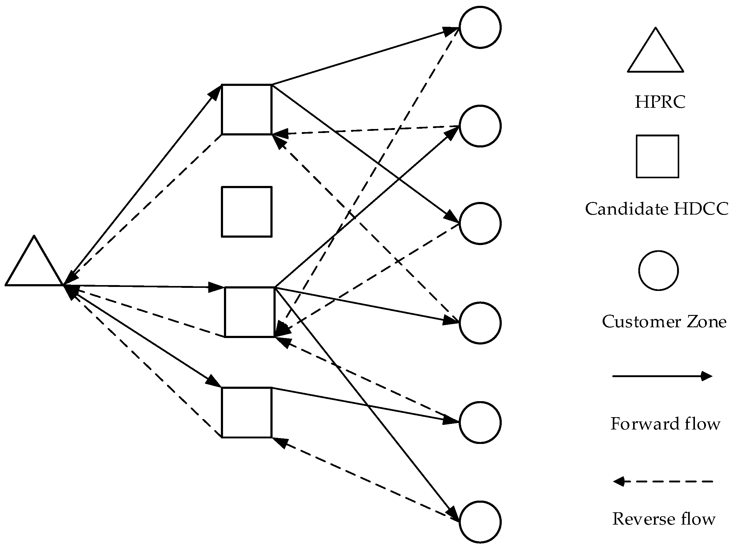
This paper studies a location inventory problem in a multi-echelon closed-loop supply chain that consists of a hybrid production-recovery center (HPRC), multiple hybrid distribution-collection centers (HDCCs), and many customer zones. In such an integrated network, business decisions at HPRC and HDCCs are considered and optimized jointly. This is very helpful for cost savings and pollution reduction [44], and hence will significantly improve the sustainability of the business.
As shown in Figure 1, the logistics flows in the primary and secondary markets are carried by a same set of facilities. In the forward flow, an HDCC will order new and refurbished products from the HPRC and fulfill the demand in the customer zones to which it is assigned. In the reverse flow, it will collect returns from those customer zones in both primary and secondary markets. In this study, the locations of customer zones are predefined and fixed, but the locations of HDCCs will be selected and optimized. The distance between HDCCs and customer zones is Euclidean distance.
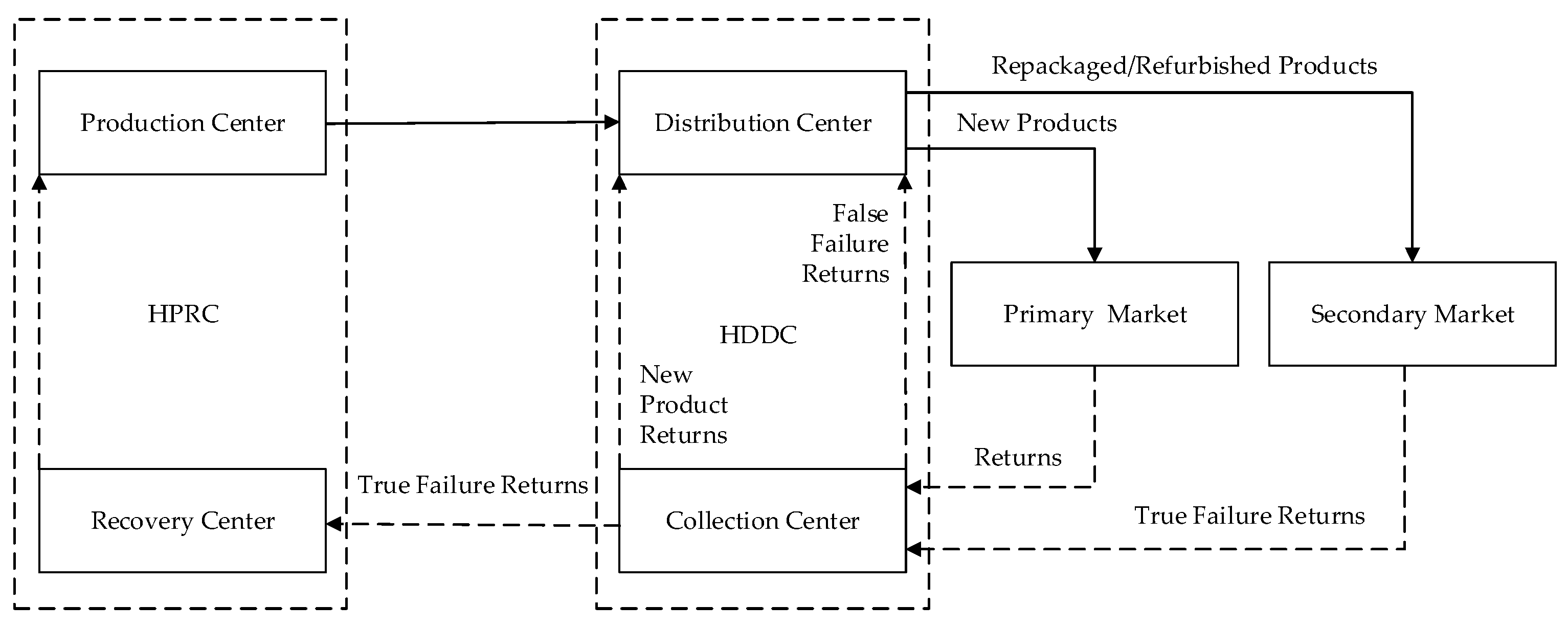
In the primary market, a returned product will be inspected at an HDCC and processed according to the inspection result. If it is a new item that is never used or opened, it will be sold to the primary market again. If the item is used but does not have any quality issues, it will be reconditioned (e.g., cleaning, repackaging, etc.) and then sold to the secondary market. If the item is used and defective, then it will be shipped to the HPRC for refurbishment.
In the secondary market, we assume that only defective products can be returned, so that all returned products will be shipped to the HPRC for refurbishment after they are inspected at HDCCs. Besides ordering refurbished products from the HPRC, the HDCC also uses two types of products from the primary market as the supply to the secondary market, which are new products whose original packages are damaged in transit or the returned used products that are not defective. Figure 2 illustrates the business processes in the closed-loop supply chain under study.
In this paper, a mixed-integer nonlinear programming (MINLP) model is formulated to minimize the total cost in such a CLSC, and the following decisions will be optimized simultaneously by solving this model:
- HDCC location selection;
- Assignment of customer zones to HDCCs in the forward logistics flow;
- Assignment of HDCCs to customer zones in the reverse logistics flow;
- Number of orders per year.
3.2. Notations
Sets
| I | set of candidate HDCC locations; |
| J | set of customer zones; |
Parameters
| ai | fixed (annual) cost of locating a HDCC at i, for each i ∈ I; |
| bi | fixed administrative and handling cost of placing an order at HDCC i to the HPRC, for each i ∈ I; |
| ci | fixed cost per shipment from the HPRC to HDCC i, for each i ∈ I; |
| dij | shipment cost per unit of product between HDCC i and customer j, for each i ∈ I and j ∈ J; |
| ei | shipment cost per unit of product between the HPRC and HDCC i, for each i ∈ I; |
| fi | inspection cost per unit of product at HDCC i, for each i ∈ I; |
| gi | processing (repackaging) cost per unit of used product without quality issues at HDCC i, for each i ∈ I; |
| hi | (annual) holding cost per unit of product at HDCC i, for each i ∈ I; |
| k | recovery cost per unit of used product with quality issues at the HPRC; |
| l | order lead time (in days) at HDCCs; |
| q1 | return rate of new products in the primary market; |
| q2 | return rate of refurbished products in the secondary market; |
| μj,1 | mean (daily) demand for new products in customer zone j, for each j ∈ J; |
| μj,2 | mean (daily) demand for refurbished products in customer zone j, for each j ∈ J; |
| variance of (daily) demand for new products in customer zone j, for each j ∈ J; | |
| variance of (daily) demand for refurbished products in customer zone j, for each j ∈ J; | |
| α | desired percentage of demand satisfied (service level); |
| zα | standard normal deviate such that ; |
| λ | working days per year; |
| β | percentage of used products without quality issues in total returns in the primary market; |
| γ | percentage of used products with quality issues in total returns in the primary market; |
| θ | percentage of returns of new products in the primary market (i.e., ); |
| δ | percentage of new products whose packages are damaged in transit. |
Decision variables
| Xi | 1 if a HDCC is opened at location i, 0, otherwise; |
| Yij | 1 if customer zone j is assigned to HDCC i in the forward flow, 0, otherwise; |
| Zji | 1 if HDCC i is assigned to customer zone j in the reverse flow, 0, otherwise. |
3.3. Mathematical Formulation
The objective function of the MINLP model is to minimize the total cost in the closed-loop system under study, and it is composed of five main components:
- Location cost, i.e., the cost of opening and operating HDCCs;
- Shipping cost from HDCCs to customer zones;
- Safety stock cost;
- Inventory cost which covers working and other inventories;
- Return cost which includes all the costs associated with returns in the primary and secondary markets.
3.3.1. Location Cost
The location cost (CL) is expressed by
3.3.2. Shipping Cost from HDCCs to Customer Zones
In the primary and secondary markets, the total annual shipping cost from HDCCs to customer zones is expressed by
3.3.3. Safety Stock Cost
According to the risk pooling effect [45], the probability of stock-out will be less than or equal to α if the amount of safety stock is . Therefore, in the primary and secondary markets, the annual cost of safety stock can be calculated by
3.3.4. Inventory Cost
In this study, we assume that HDCCs use a (Q, r) inventory model with type I service to manage their inventories because it is common to approximate the (Q, r) model with the order quantity determined by an economic order quantity (EOQ) model [46]. The order frequency and quantities at an HDCC are determined by the expected demands in the customer zones that are served by the HDCC. Let ni be the number of orders from HDCC i to the HPRC in a year. The total inventory cost at a HDCC consists of:
- Working inventory cost
- Order cost
In the primary and secondary markets, order cost at HDCC i is expressed by bini.
- Shipping cost from the HPRC to HDCCs.
In the primary and secondary markets, shipping cost from the HPRC to HDCC i is expressed by
- Holding cost of the working inventory
In the primary and secondary markets, holding cost of the working inventory at HDCC i is expressed by
- 2.
- Return inventory cost
Besides working inventory, returned products will also add to the total inventory and hence lead to additional costs. In this study, we assume that returned products without quality issues will stay in inventory and be resold in the next period after they are collected from customer zones, but those with quality issues will be shipped to the HPRC and will not account for the inventory cost. In this case, returned inventory cost in the primary market can be calculated by
- 3.
- Total inventory cost
The total inventory cost in the primary and secondary markets is aggregated as
Obviously, CINV is convex with respect to ni. Taking the partial derivative of CINV to ni, then the optimal quantity of ni can be calculated by
Therefore, the total inventory cost in the primary and secondary markets can be rewritten as
3.3.5. Return Cost
Return cost consists of the expenses caused by returns. In the primary market, it consists of: (a) Inspection cost, which is the cost of inspecting returned products at HDCCs; (b) Repackaging cost, which is the cost of repackaging or reconditioning returned products that have no quality issues at HDCCs; (c) Recovery cost, which is the cost of refurbishing returned products that have quality issues at the HPRC; (d) Shipping cost of returned products from customer zones to HDCCs; and (e) Shipping cost of returned products from HDCCs to the HPRC. In the secondary market, the cost terms are mostly the same except the repackaging cost because only defective products can be returned in this market. Therefore, return cost can be calculated as follows:
- 1.
- Inspection cost
In the primary and secondary markets, the total inspection cost at HDCCs is given by
- 2.
- Repackaging cost
In the primary market, the total repackaging cost at HDCCs is given by
- 3.
- Recovery cost
In the primary and secondary markets, the total recovery cost at the HPRC is given by
- 4.
- Shipping cost from customers to HDCCs
In the primary and secondary markets, the total shipment cost of returned products from customer zones to HDCCs is given by
- 5.
- Shipping cost from HDCCs to HPRC
In the primary and secondary markets, the total shipment cost of returned products from HDCCs to the HPRC is given by
Therefore, the total return cost in the closed-loop supply chain can be calculated as follows:
3.3.6. MINLP Model
Let CTOT be the total cost in the closed-loop supply chain. Then, the LIP problem under study can be formulated as follows:
subject to
The objective function shown in Equation (1) is to minimize the total annual cost in the closed-loop system under study. Constraint (2) means that at least one HDCC will be established in this system. Constraint (3) means that a customer zone will be assigned to one HDCC exactly in the forward flow. Constraint (4) means that a HDCC will be assigned to one customer zone exactly in the reverse flow. Constraints (5) and (6) mean that a HDCC will provide services in the forward and reverse logistics networks, respectively, only if it is established. Constraints (7) and (8) mean that, once it is established, an HDCC must serve at least one customer zone in the forward and reverse logistics networks, respectively. Constraint (9) means that a HDCC cannot collect returned products in the reverse flow unless it is functional in the forward logistics. Constraints (10)–(12) mean that decisions variables are binary in this model.
4. Solution Approach
The location problem is NP-hard in general [47], and the joint location-inventory problems are usually more complex to solve. Therefore, evolutionary algorithms (EAs) are extensively used to solve LIPs in the literature [39,40]. Differential evolution (DE) [48] shares similar characteristics with other population-based EAs, and it has been widely applied to solve global optimization problems [49] such as LIPs because of its simplicity and effectiveness [40]. Although DE has a strong global search ability, its performance is not always guaranteed because of its prematurity and weak local search ability. To obtain a more robust and effective approach, an improved self-adaptive differential evolution (ISaDE) algorithm is designed to overcome those shortcomings. The parameters and operators in the ISaDE algorithm are introduced in Table 1.
Generally, DE contains four operations: initialization, mutation, crossover, and selection. After initialization, DE enters a loop of mutation, crossover and selection operations to update the population. The main operations in ISaDE are described in details as follows.
4.1. Initialization
4.1.1. Individuals
In a DE scheme, individuals in a population represent the candidate solutions to an optimization problem, and they will evolve to better solutions iteratively. Therefore, the form of individuals plays an important role in the development of a DE algorithm, and an encoding-decoding scheme is needed to translate individuals in a population to the solutions to the MINLP model, and vice versa. In ISaDE, an individual is represented by a vector with 2N elements, where the first N elements are related to the forward logistics flow, and the last N elements are related to the reverse flow. Mathematically, an individual is represented by Equation (13):
For example, HDCCs will be established at four candidate locations to serve ten customer zones, and hence an individual can be encoded as {1, 4, 4, 1, 1, 2, 4, 2, 2, 4, 2, 2, 1, 2, 1, 4, 2, 1, 1, 1}. In this example, the first ten entries in this vector means that in the forward logistics flow, the HDCC at location 1 (or HDCC 1) will server customer zones {1, 4, 5}, HDCC 2 will serve customer zones {6, 8, 9}, and the HDCC 4 serves customer zones {2, 3, 7,10}. The last ten entries in this vector means that, in the reverse logistics, HDCC 1 will collect returns from customer zones {3, 5, 8, 9, 10}, HDCC 2 will collect returns from customer zones {1, 2, 4, 7}, and HDCC 4 will collect returns from customer zones {6}. Therefore, decision variables in the MINLP model, i.e., Xi, Yij and Zji, can be represented by individuals in ISaDE.
4.1.2. Population Initialization
Given i (1 ≤ i ≤ P), the initial population can be generated by Equation (14):
where round is the rounding function, r(j) ∈ [0,1] is the jth realization of a uniform random variable. is a vector whose entries are the unique values of in ascending order, xL and xU are the lower and upper bound of respectively.
Practically, xL and xU mean the minimum and maximum numbers of HDCCs to be established. Obviously, xL is equal to 1, and xU is the number of candidate HDCC locations. The encoding scheme of the last N entries ensures that an HDCC cannot become a collection center in the reverse logistics unless it functions as a distribution center in the forward logistics.
4.2. Mutation
In DE algorithms, the mutation operation plays a vital role because of its importance to the search capability and convergence rate. The basic mutation scheme (DE/rand/1) produces a new vector by adding a weighted difference of two randomly selected vectors to a random vector in generation g. In this study, DE/rand/1 is adopted as the basic mutation strategy, and it can be expressed by Equation (15):
where i ≠ r1 ≠ r2 ≠ r3, r1, r2, r3 are randomly selected from {1, 2, …, P}, round is the rounding function, and F ∈ [0,1] is the mutation factor that controls the amplification of differential variation.
To avoid prematurity and accelerate convergence, we design a new adaptive mechanism to choose F randomly at each iteration, and it is introduced by Equation (16) in the mutation operation:
where rand1 and rand2 are two random variables that are uniformly distributed on [0,1], τ1 is a constant value that represents the probability of updating parameters, Fmin and Fmax is the minimum and maximum F, respectively. Note that, in our experiments, we set Fmin = 0.1, Fmax = 0.9 and τ1 = 0.9.
4.3. Crossover
In ISaDE, the crossover operation is used to generate new individuals and increase the diversity of a population. After the mutation operation, a trial vector will be generated from a mutate vector and target vector by applying the crossover operator. To increase the population diversity and strengthen the searching abilities, we introduce a novel crossover operator in ISaDE. The trial vector is generated by Equation (17):
where k ∈ [1, 2,…, P] is a random integer, r(j) ∈ [0,1] is a random number that is generated from the uniform distribution, and CR ∈ [0,1] is the crossover factor that controls the amplification of differential variation.
To further increase the diversity of a population and improve the robustness of the algorithm, an adaptive mechanism is also introduced in the crossover operator. More specifically, the crossover factor CR is adaptively changed according to Equation (18):
where rand3 and rand4 are two random variables that are uniformly distributed on [0,1], and τ2 is a constant that represents the probability of updating parameters. Note that we have τ2 = 0.9 in this study.
4.4. Feasibility Correction
The crossover and mutation operations may create new individuals that are equivalent to infeasible solutions to the MINLP model by violating Constraint (9). To avoid this issue, a screening mechanism is needed to remove infeasible solutions that are generated by ISaDE. In this study, the feasibility correction procedure is designed as follows: A new individual will be checked after it is generated. If it equals to a solution that indicates an HDCC will be established only for collecting returns in the reverse flow, it will be substituted by a new individual that is randomly generated by Equation (12).
4.5. Selection
After a new population is generated from its predecessor by mutation, crossover, and feasibility correction, a selection operation will be performed by evaluating the objective values of all trial vectors because the new population needs to be better than its predecessor. In ISaDE, the objective value of an trial vector will be compared to the corresponding target vector by using a greedy criterion [48], and the selection operation can be expressed by Equation (19):
where is the objective function shown in Equation (1).
4.6. Stopping Criteria
The operations above will be repeated iteratively until a termination criterion is satisfied. The execution of ISaDE will be terminated if any of the two criteria below is satisfied:
- Stop if no better solution is obtained in consecutive K iterations (where K is a pre-defined counter value);
- Stop if the maximum number of iterations, which is denoted by G, is reached.
4.7. Algorithm Flow
The steps in ISaDE are summarized as follows:
Step 1: Initialization. Create P individuals randomly;
Step 2: Set iteration index G to 1;
Step 3: Set initial target index K to 1;
Step 4: Calculate objective values of individuals in the population. Note that the objective is given by Equation (1);
Step 5: Mutation operation: update mutation factor F using Equation (14) and generate mutation vector by Equation (13);
Step 6: Crossover operation: update crossover factor CR using Equation (16) and generate trail vector by Equation (15);
Step 7: Feasibility correction: identify and remove the individuals that are equivalent to infeasible solutions;
Step 8: Selection operation: generate a new population by Equation (17) and calculate objective values;
Step 9: Stop the algorithm if any stopping criterion is satisfied. Otherwise, go to Step 4.
5. Numerical Experiment
This section presents computational results to study related parameters and validate ISaDE. First, control parameters F and CR are analyzed because they are important for ISaDE. Next, sensitivity analysis is conducted to measure the impact of cost parameters. Last, ISaDE is compared with Lingo 11 to validate its effectiveness and efficiency.
In this study, the locations of candidate HDCCs and customer zones are randomly generated on a grid with the size of (0,100) × (0,100), and the parameters in the MINLP model are shown in Table 2. All experiments were implemented by using Java JDK 1.7 on a Windows PC (AMD A10-9600P RADEON R5, 10 COMPUTE CORES 4C+6G 2.40GHz; RAM: 4.00 GB DDR; OS: Windows 10).
5.1. Parameter Analysis
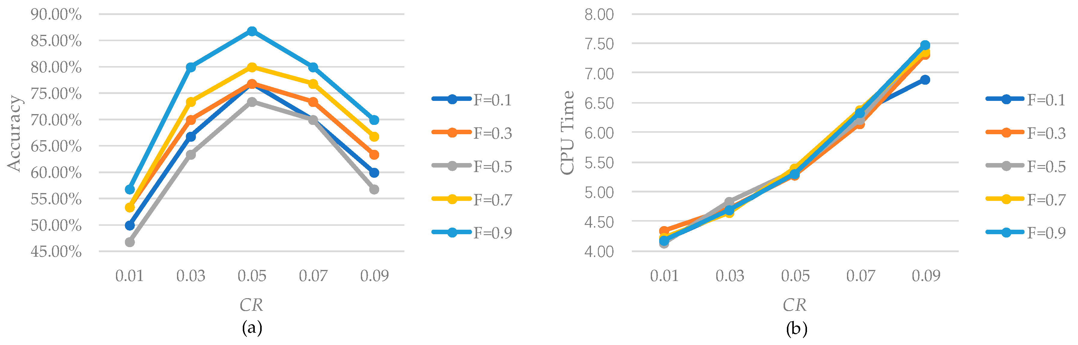
In ISaDE, mutation factor F and crossover probability CR are two important parameters that have a significant impact on solution accuracy and time efficiency. To evaluate their effects, we use an example network that consists of 10 candidate HDCC locations and 100 customer zones, and execute the algorithm 30 times under each combination of parameters by setting P = 5N. The numerical results are shown in Figure 3.
In Figure 3, the performance of ISaDE is evaluated by (a) solution accuracy in terms of the probability of finding the optimal solution, and (b) time efficiency in terms of CPU Time. From Figure 3, we can see that the performance of ISaDE can be affected by F and CR individually or jointly. Figure 3a shows that (i) as CR increases, solution accuracy will first increase and then decrease, and the best solution accuracy is achieved when CR = 0.05, and (ii) as F increases, solution accuracy will always increase, and the best solution accuracy is achieved when F = 0.9. Figure 3b shows that time efficiency will always increase as CR increases, but is almost identical under the different values of F. Overall, ISaDE has the best performance when F = 0.9 and CR = 0.05, and hence this setting will be used in the subsequent analysis.
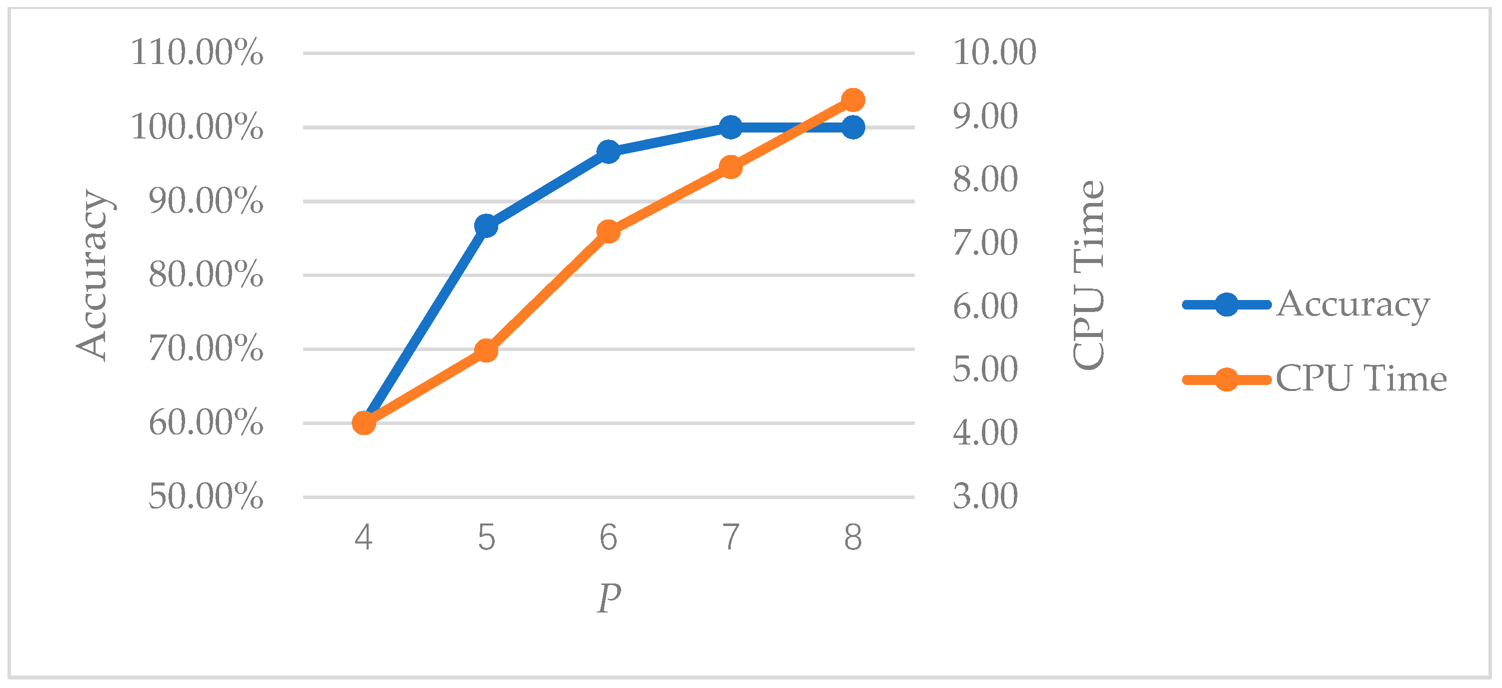
Besides parameters F and CR, population size P is another important parameter that can affect the robustness and effectiveness of ISaDE. Therefore, P is also tested at different values by using the example above, and the results are shown in Figure 4. We can see that, as P increases, both solution accuracy and CPU time will increase monotonically. This means that a larger population size will lead to a more stable solution, but it will also increase the runtime of the algorithm. Obviously, ISaDE has the best overall performance when P = 6N or P = 7N, and P = 6N will be used in the subsequent analysis.
5.2. Sensitivity Analysis
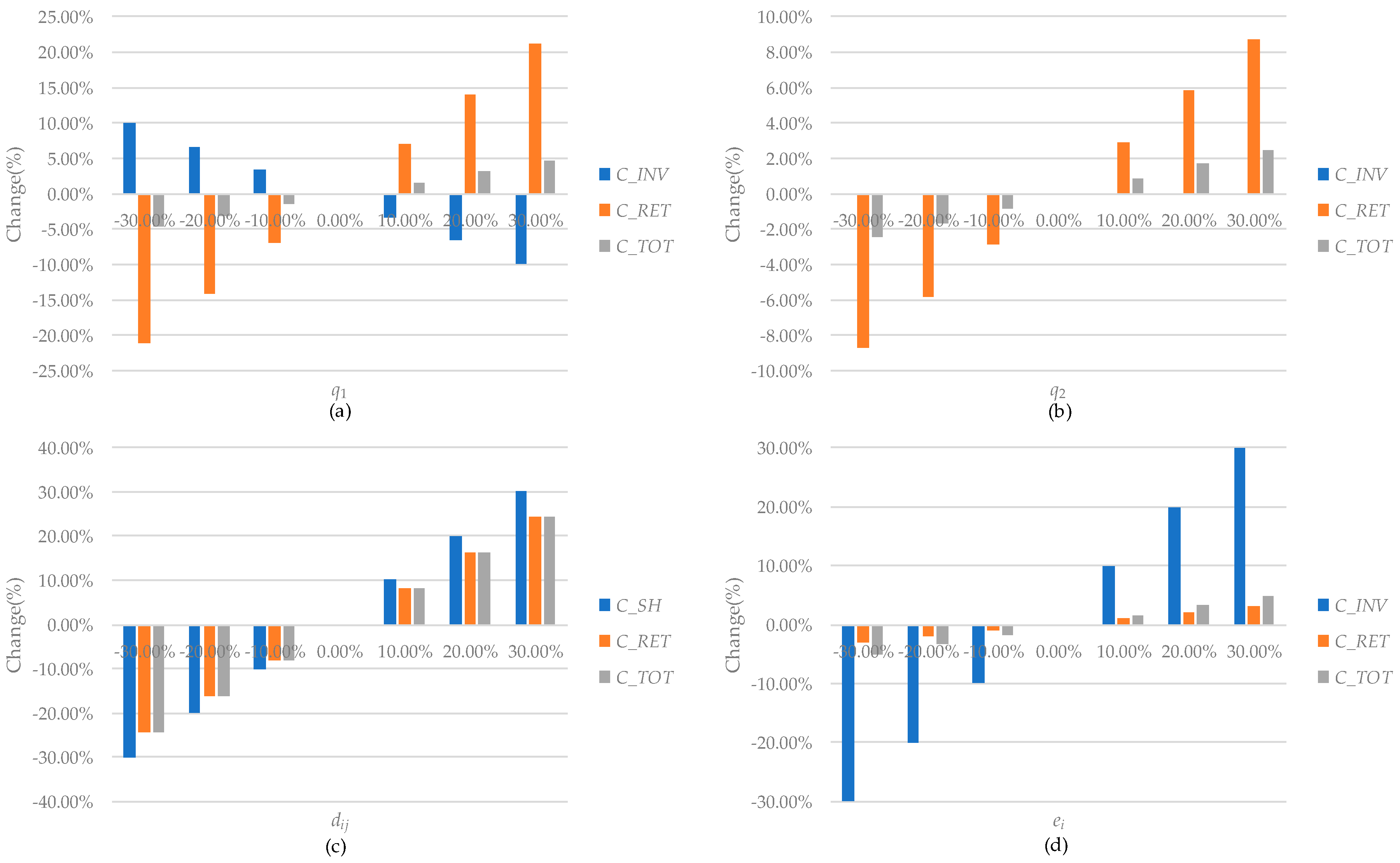
Sensitivity analysis is an effective means to study how the change of a parameter affects the output of a system. In practice, it provides an efficient way for decision-makers to identify main drivers to improve their supply chain systems. In this study, sensitivity analysis is conducted to measure the impact of the changes of business parameters on the optimal solution. For dij, ei, q1 and q2, each parameter is analyzed individually by varying its value within the range of [−30%, 30%] and fixing the other paramaters. The numerical results are shown in Figure 5, and we can draw the conclusions below:
- (1)
- From Figure 5a, we can see that, as q1 increases, inventory cost CINV will decrease but return cost CRET will increase significantly, and hence total cost CTOT will increase slightly. We can also see that, as q1 decreases, inventory cost CINV will increase but return cost CRET will decrease significantly, and hence total cost CTOT will decrease slightly. When q1 varies from −30% to 30%, the ranges of the changes of CINV, CRET, and CTOT are [−9.89%, 9.89%], [−21.09%, 21.09%] and [−4.65%, 4.65%], respectively.
- (2)
- From Figure 5b, we can see that when q2 changes, return cost CRET will change reversely and the other individual costs will remain the same. Hence, total cost CTOT will increase. When q2 varies from −30% to 30%, the ranges of the changes of CRET and CTOT are [−8.72%, 8.72%] and [−2.48%, 2.48%], respectively.
- (3)
- From Figure 5c, we can see that, as dij increases, shipping cost CSH and return cost CRET will increase significantly, and, as dij decreases, CSH and CRET will decrease significantly. When dij changes, although the other individual costs will remain the same, total cost CTOT will still change significantly because of the changes of CSH and CRET. When dij varies from −30% to 30%, the ranges of the changes of CSH, CRET, and CTOT are [−30.00%, 30.00%], [−24.42%, 24.42%] and [−24.31%, 24.31%], respectively.
- (4)
- From Figure 5d, we can see that, as ei increases, inventory cost CINV and return cost CRET will increase significantly and slightly, respectively. We can also see that, as ei decreases, inventory cost CINV and return cost CRET will decrease significantly and slightly, respectively. When ei varies from −30% to 30%, the ranges of the changes of CINV, CRET, and CTOT are [−29.86%, 29.86%], [−3.03%, 3.03%] and [−4.94%, 4.94%], respectively.
In this study, sensitivity analysis is also conducted on bi, ci, hi, gi, fi, k and δ, but the numerical results are not shown because their impacts are not significant.
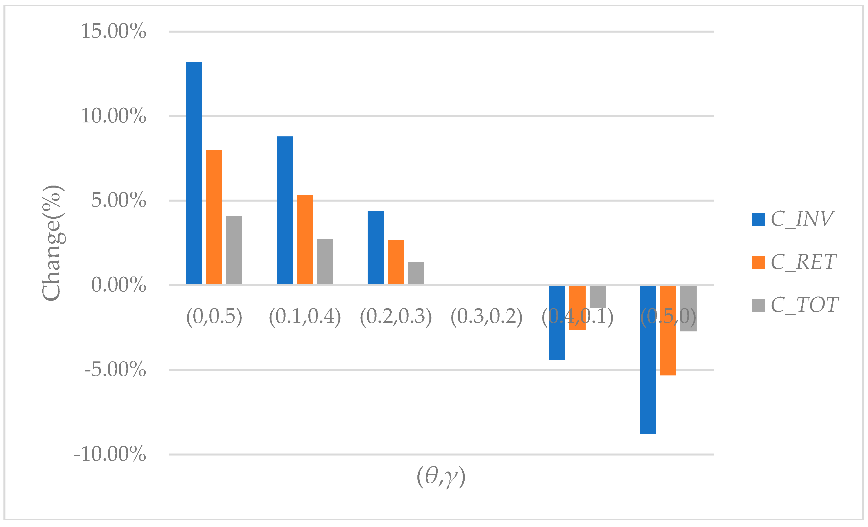
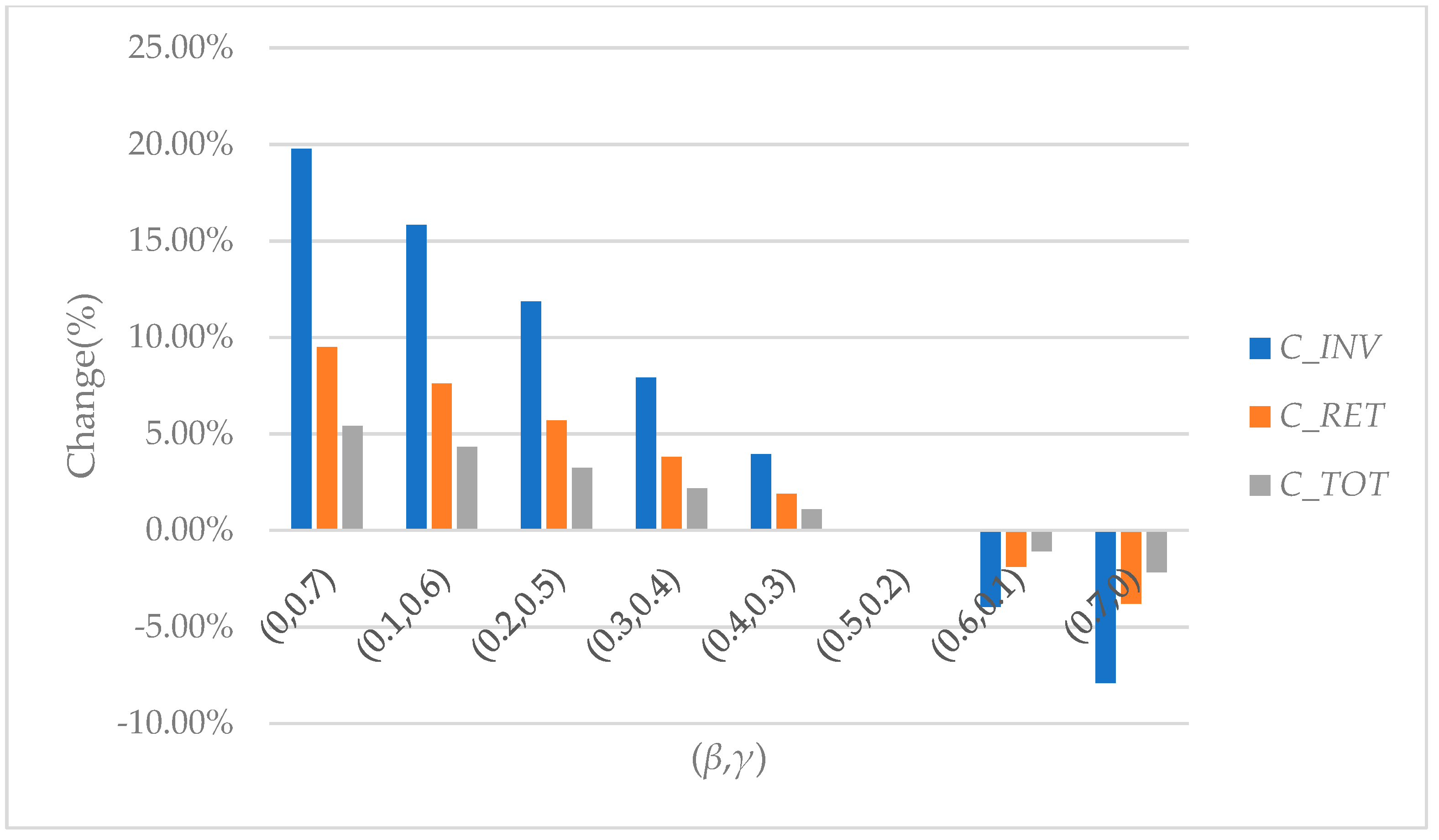
Although it is well known that returns are causing tremendous loss in the industry, it is not clear how the loss is driven by different types of returns. To support important business decisions such as return policies, it will be greatly beneficial to analyze the sensitivity of the cost functions to different types of returns in the primary market. Since the sum of θ, β, and γ always equals 1, a parameter cannot be changed without affecting others. Therefore, sensitivity analysis is conducted on θ, β, γ in pairs, and the numerical results are shown in Figure 6, Figure 7 and Figure 8.
From Figure 6, we can see that when γ is fixed, the change of (θ, β) has a great impact on the inventory, return and total costs, and those costs will decrease significantly as θ increases and β decreases. More specifically, when γ = 0.2 and (θ, β) changes from (0, 0.8) to (0.8, 0), the ranges of the changes of CINV, CRET, and CTOT are [1.32%, −2.20%], [2.28%, −3.80%] and [0.83%, −1.38%], respectively. From Figure 7, we can see that when β is fixed, the change of (θ, γ) has a great impact on the inventory, return and total costs, and those costs will decrease significantly as θ increases and γ decreases. More specifically, when β = 0.5 and (θ, γ) changes from (0, 0.5) to (0.5, 0), the ranges of the changes of CINV, CRET, and CTOT are [13.19%, −8.79%], [7.98%, −5.32%] and [4.07%, −2.72%], respectively. From Figure 8, we can see that when θ is fixed, the change of (β, γ) has a significant impact on the return and total costs. More specifically, when θ = 0.3 and (β, γ) changes from (0, 0.7) to (0.7, 0), the ranges of the changes of CINV, CRET, and CTOT are [19.78%, −7.91%], [9.50%, −3.80%] and [5.41%, −2.16%], respectively.
5.3. Performance Comparison
In this sub-section, ISaDE is compared with Lingo 11 to validate its performance in terms of solution accuracy and time efficiency, and the numerical results are shown in Table 3. To compare their performances thoroughly, ISaDE and Lingo are tested on a set of problems in small (i.e., 20 × 5, 40 × 5, 60 × 5), medium (i.e., 80 × 10, 100 × 10, 120 × 10) and large (i.e., 140 × 15, 160 × 15, 180 × 15) sizes. Moreover, there are two instances for each size, and the coordinates of HDCC locations and customer zones are different in the two instances. For each problem, ISaDE is executed 30 times, but Lingo is executed only once because of their different natures. From Table 3, we can see that ISaDE is much faster than Lingo for all instances, and hence it has great time efficiency to solve those problems. Moreover, for each instance, the mean optimal value from 30 runs of ISaDE is almost identical to the optimal value given by Lingo, which indicates that ISaDE has a good capability to search the global optimums. We can also see that the standard deviation of the optimal values given by ISaDE is very small in all test cases, and this indicates that ISaDE has a good consistency to find the optimal solution. Therefore, we can conclude that ISaDE is a robust and efficient approach to solve the LIP problem under study.
6. Conclusions
There is growing interest among researchers in the concept of sustainability [50], and closed-loop supply chain (CLSC) is a sustainable design that attracts a lot of attention due to increasing environmental concerns and significant economic impact of customer returns. In practice, CLSCs provide an effective means to collect customer returns and recycle used items, while secondary markets are important channels to sell those products. In this paper, we study a location-inventory problem (LIP) in a CLSC by considering the secondary market, and our main contributions are summarized as follows:
- This paper considers both primary and secondary markets for the operations of a CLSC, and it fills the gap in the existing CLSC literature that rarely considers secondary markets.
- A mixed-integer nonlinear programming model is developed to optimize facility location and inventory management decisions jointly, and the logistics flows between the primary and secondary markets are modelled precisely. Since LIPs are NP-hard, an improved self-adapting differential evolution algorithm is designed to solve such problems efficiently. The numerical experiments show that this algorithm is a robust and effective approach that has a better performance than Lingo.
- This paper also provides valuable managerial insight into how to improve the sustainability and finance performance of the closed-loop system under study. In this study, the impact of important business parameters on cost functions is measured and evaluated quantitatively, and it is greatly beneficial for decision makers to identify the key factors in their business and improve their supply chains accordingly.
This study can be extended in several directions. First, many other research problems or business processes can be incorporated to extend this study. For example, this problem can be extended to a location-inventory-routing problem (LIRP) by incorporating vehicle routing problem. Second, we assume that the assignment between HDCCs and customer zones are the same in both primary and secondary markets in this study, but it will be more flexible to relax this assumption and consider different assignments in different markets. Finally, a parameter analysis approach is adopted to achieve the best performance of ISaDE, but it will be more helpful to design a mechanism to tune the parameters automatically.
Author Contributions
H.G. developed the mathematical model, designed the experiments, and co-drafted the manuscript. C.L. supervised the whole research work and provided constructive suggestions to improve the research and manuscript. Y.Z. proposed the research problem, involved in model development, and co-drafted the manuscript. C.Z. co-drafted, reviewed, and edited the manuscript. M.L. contributed to the research problem and literature review. C.L. and Y.Z. revised the manuscript. All authors have read and approved the manuscript.
Acknowledgments
This research was supported by the National Natural Science Foundation of China under Grant Nos. 71672074 and 71772075.
Conflicts of Interest
The authors declare no conflict of interest.
References
- Choi, T.-M.; Guo, S. Responsive supply in fashion mass customisation systems with consumer returns. Int. J. Prod. Res. 2017, in press. [Google Scholar] [CrossRef]
- National Retail Federation. 2015 Consumer Returns in the Retail Industry. Available online: https://nrf.com/sites/default/files/Images/Media%20Center/NRF%20Retail%20Return%20Fraud%20Final_0.pdf (accessed on 18 April 2018).
- Rao, S.; Rabinovich, E.; Raju, D. The role of physical distribution services as determinants of product returns in Internet retailing. J. Oper. Manag. 2014, 32, 295–312. [Google Scholar] [CrossRef]
- E-Commerce Product Return Rate—Statistics and Trends. Available online: https://www.invespcro.com/blog/ecommerce-product-return-rate-statistics/ (accessed on 18 April 2018).
- Mostard, J.; Teunter, R. The newsboy problem with resalable returns: A single period model and case study. Eur. J. Oper. Res. 2006, 169, 81–96. [Google Scholar] [CrossRef]
- Al-Salem, M.; Diabat, A.; Dalalah, D.; Alrefaei, M. A closed-loop supply chain management problem: Reformulation and piecewise linearization. J. Manuf. Syst. 2016, 40, 1–8. [Google Scholar] [CrossRef]
- Souza, G.C. Closed-loop supply chains: A critical review, and future research. Decis. Sci. 2013, 44, 7–38. [Google Scholar] [CrossRef]
- Diabat, A.; Abdallah, T.; Henschel, A. A closed-loop location-inventory problem with spare parts consideration. Comput. Oper. Res. 2015, 54, 245–256. [Google Scholar] [CrossRef]
- Liu, H.H.; Lei, M.; Huang, T.; Leong, G.K. Refurbishing authorization strategy in the secondary market for electrical and electronic products. Int. J. Prod. Econ. 2018, 195, 198–209. [Google Scholar] [CrossRef]
- Chen, J.; Chen, B.T.; Li, W. Who should be pricing leader in the presence of customer returns? Eur. J. Oper. Res. 2018, 265, 735–747. [Google Scholar] [CrossRef]
- Turki, S.; Didukh, S.; Sauvey, C.; Rezg, N. Optimization and analysis of a manufacturing–remanufacturing-transport-warehousing system within a closed-loop supply chain. Sustainability 2017, 9, 561. [Google Scholar] [CrossRef]
- Hasani, A.; Zegordi, S.H.; Nikbakhsh, E. Robust closed-loop supply chain network design for perishable goods in agile manufacturing under uncertainty. Int. J. Prod. Res. 2012, 50, 4649–4669. [Google Scholar] [CrossRef]
- Huang, Y.T.; Wang, Z.J. Dual-recycling channel decision in a closed-loop supply chain with cost disruptions. Sustainability 2017, 9, 2004. [Google Scholar] [CrossRef]
- Xu, Z.; Pokharel, S.; Elomri, A.; Mutlu, F. Emission policies and their analysis for the design of hybrid and dedicated closed-loop supply chains. J. Clean. Prod. 2017, 142, 4152–4168. [Google Scholar] [CrossRef]
- Son, D.; Kim, S.; Park, H.; Jeong, B. Closed-loop supply chain planning model of rare metals. Sustainability 2018, 10, 1061. [Google Scholar] [CrossRef]
- Jabbarzadeh, A.; Haughton, M.; Khosrojerdi, A. Closed-loop supply chain network design under disruption risks: A robust approach with real world application. Comput. Ind. Eng. 2018, 116, 178–191. [Google Scholar] [CrossRef]
- Choi, T.M.; Li, Y.; Xu, L. Channel leadership, performance and coordination in closed loop supply chains. Int. J. Prod. Econ. 2018, 146, 371–380. [Google Scholar] [CrossRef]
- Taleizadeh, A.A.; Sane-Zerang, E.; Choi, T.M. The effect of marketing effort on dual channel closed loop supply chain systems. IEEE Trans. Syst. Man Cybern. Syst. 2016, 48, 265–276. [Google Scholar] [CrossRef]
- Govindan, K.; Soleimani, H.; Kannan, D. Reverse logistics and closed-loop supply chain: A comprehensive review to explore the future. Eur. J. Oper. Res. 2015, 240, 603–626. [Google Scholar] [CrossRef] [Green Version]
- Masoudipour, E.; Amirian, H.; Sahraeian, R. A novel closed-loop supply chain based on the quality of returned products. J. Clean. Prod. 2017, 151, 344–355. [Google Scholar] [CrossRef]
- Kannan, D.; Garg, K.; Jha, P.C.; Diabat, A. Integrating disassembly line balancing in the planning of a reverse logistics network from the perspective of a third party provider. Ann. Oper. Res. 2017, 253, 353–376. [Google Scholar] [CrossRef]
- Guo, H.; Zhang, Y.; Zhang, C.; Liu, Y.; Zhou, Y. Location-inventory decisions for closed-loop supply chain management in the presence of secondary market. Ann. Oper. Res. 2018. under review. [Google Scholar]
- Angelus, A.A. multiechelon inventory problem with secondary market sales. Manag. Sci. 2011, 57, 2145–2162. [Google Scholar] [CrossRef]
- Xiong, Y.; Zhao, P.; Xiong, Z.K.; Li, G.D. The impact of product upgrading on the decision of entrance to a secondary market. Eur. J. Oper. Res. 2016, 252, 443–454. [Google Scholar] [CrossRef]
- Huang, X.M.; Gu, J.W.; Ching, W.K.; Siu, T.K. Impact of secondary market on consumer return policies and supply chain coordination. Omega 2014, 45, 57–70. [Google Scholar] [CrossRef]
- Lee, H.; Whang, S. The impact of the secondary market on the supply chain. Manag. Sci. 2002, 48, 719–731. [Google Scholar] [CrossRef]
- He, Y.J.; Zhang, J. Random yield supply chain with a yield dependent secondary market. Eur. J. Oper. Res. 2010, 206, 221–230. [Google Scholar] [CrossRef] [Green Version]
- Melo, M.T.; Nickel, S.; Saldanha-Da-Gama, F. Facility location and supply chain management—A review. Eur. J. Oper. Res. 2009, 196, 401–412. [Google Scholar] [CrossRef]
- Farahani, R.Z.; Bajgan, H.R.; Fahimnia, B.; Kaviani, M. Location-inventory problem in supply chains: A modelling review. Int. J. Prod. Res. 2015, 53, 3769–3788. [Google Scholar] [CrossRef]
- Guo, H.; Li, C.; Zhang, Y.; Zhang, C.; Wang, Y. A nonlinear integer programming model for integrated location, inventory and routing decisions in a closed-loop supply chain. Complexity 2018. under review. [Google Scholar]
- Daskin, M.S.; Coullard, C.R.; Shen, Z.J.M. An inventory-location model: Formulation, solution algorithm and computational results. Ann. Oper. Res. 2002, 110, 83–106. [Google Scholar] [CrossRef]
- Shen, Z.J.M.; Coullard, C.; Daskin, M.S. A joint location-inventory model. Transp. Sci. 2003, 37, 40–55. [Google Scholar] [CrossRef]
- Berman, O.; Krass, D.; Tajbakhshb, M.M. A coordinated location-inventory model. Eur. J. Oper. Res. 2012, 217, 500–508. [Google Scholar] [CrossRef]
- Diabat, A.; Dehghani, E.; Jabbarzadeh, A. Incorporating location and inventory decisions into a supply chain design problem with uncertain demands and lead times. J. Manuf. Syst. 2017, 43, 139–149. [Google Scholar] [CrossRef]
- Shahabi, M.; Unnikrishnan, A.; Jafari-Shirazi, E.; Boyles, S.D. A three level location-inventory problem with correlated demand. Transp. Res. Part B Methodol. 2014, 69, 1–18. [Google Scholar] [CrossRef]
- Meissner, J.; Senicheva, O.V. Approximate dynamic programming for lateral transshipment problems in multi-location inventory systems. Eur. J. Oper. Res. 2018, 265, 49–64. [Google Scholar] [CrossRef]
- Dai, Z.; Aqlan, F.; Zheng, X.; Gao, K. A location-inventory supply chain network model using two heuristic algorithms for perishable products with fuzzy constraints. Comput. Ind. Eng. 2018, in press. [Google Scholar] [CrossRef]
- Farahani, M.; Shavandi, H.; Rahmani, D. A location-inventory model considering a strategy to mitigate disruption risk in supply chain by substitutable products. Comput. Ind. Eng. 2017, 108, 213–224. [Google Scholar] [CrossRef]
- Mohammad Arabzad, S.; Ghorbani, M.; Tavakkoli-Moghaddam, R. An evolutionary algorithm for a new multi-objective location-inventory model in a distribution network with transportation modes and third-party logistics providers. Int. J. Prod. Res. 2014, 53, 1038–1050. [Google Scholar] [CrossRef]
- Li, Y.H.; Guo, H.; Zhang, Y. An integrated location-inventory problem in a closed-loop supply chain with third-party logistics. Int. J. Prod. Res. 2017, in press. [Google Scholar] [CrossRef]
- Asl-Najafi, J.; Zahiri, B.; Bozorgi-Amiri, A.; Taheri-Moghaddam, A. A dynamic closed-loop location-inventory problem under disruption risk. Comput. Ind. Eng. 2015, 90, 414–428. [Google Scholar] [CrossRef]
- Zhang, Z.H.; Unnikrishnan, A. A coordinated location-inventory problem in closed-loop supply chain. Transp. Res. Part B Methodol. 2016, 89, 127–148. [Google Scholar] [CrossRef] [Green Version]
- Kaya, O.; Urek, B. A mixed integer nonlinear programming model and heuristic solutions for location, inventory and pricing decisions in a closed loop supply chain. Comput. Oper. Res. 2016, 65, 93–103. [Google Scholar] [CrossRef]
- Torabi, S.A.; Namdar, J.; Hatefi, S.M.; Jolai, F. An enhanced possibilistic programming approach for reliable closed-loop supply chain network design. Int. J. Prod. Res. 2015, 54, 1358–1387. [Google Scholar] [CrossRef]
- Eppen, G.D. Effects of centralization on expected costs in a multi-location newsboy problem. Manag. Sci. 1979, 25, 498–501. [Google Scholar] [CrossRef]
- Axsäter, S. Using the deterministic EOQ formula in stochastic inventory control. Manag. Sci. 1996, 42, 830–834. [Google Scholar] [CrossRef]
- Shen, Z.J.M. Integrated supply chain design models: A survey and future research directions. J. Ind. Manag. Optim. 2007, 3, 1–27. [Google Scholar] [CrossRef]
- Storn, R.; Price, K. Differential evolution—A simple and efficient heuristic for global optimization over continuous spaces. J. Glob. Optim. 1997, 11, 341–359. [Google Scholar] [CrossRef]
- Fu, C.M.; Jiang, C.; Chen, G.S.; Liu, Q.M. An adaptive differential evolution algorithm with an aging leader and challengers mechanism. Appl. Soft. Comput. 2017, 57, 60–73. [Google Scholar] [CrossRef]
- Dubey, R.; Gunasekaran, A.; Childe, S.J. The design of a responsive sustainable supply chain network under uncertainty. Int. J. Adv. Manuf. Technol. 2015, 80, 427–445. [Google Scholar] [CrossRef]
Figure 1.
A closed-loop supply chain system.

Figure 2.
Business processes in the closed-loop supply chain.

Figure 3.
Analysis of F and CR: (a) Solution accuracy; (b) CPU time.

Figure 4.
Analysis of P.

Figure 5.
Sensitivity analysis on individual parameters: (a) q1; (b) q2; (c) dij; (d) ei.

Figure 6.
Sensitivity analysis on (θ, β).
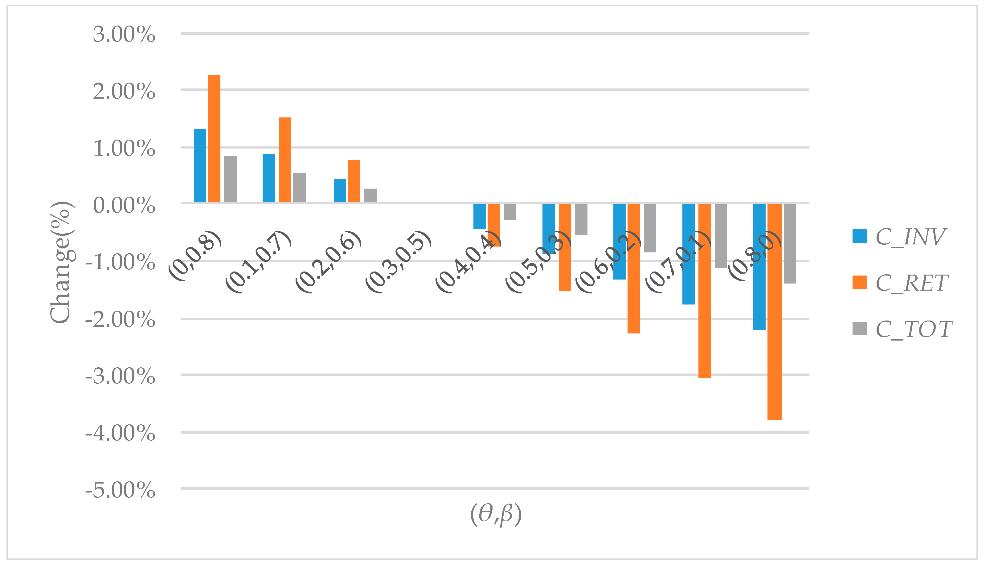
Figure 7.
Sensitivity analysis on (θ, γ).

Figure 8.
Sensitivity analysis on (β, γ).


Table 1.
ISaDE parameters.
| Notation | Explanation |
|---|---|
| P | population size |
| N | dimension (i.e., number of customer zones in this study) |
| G | maximum number of generations in an evolution process |
| Xig | solution vector for individuals i in generation g (1 ≤ i ≤ P, 1 ≤ g ≤ G) |
| Vig | mutant vector for individuals i in generation g (1 ≤ i ≤ P, 1 ≤ g ≤ G) |
| Uig | trial vector for individuals i in generation g (1 ≤ i ≤ P, 1 ≤ g ≤ G) |
| F | mutation factor |
| CR | crossover factor |
Table 2.
MINLP model parameters.
| Parameter | Value | Parameter | Value | Parameter | Value |
|---|---|---|---|---|---|
| ai | U(1000,1500) | bi | 10 | ci | 10 |
| ei | 5 | fi | 1 | gi | 1 |
| hi | 1 | k | 1 | l | 1 |
| 0.6 | 0.2 | θ | 0.3 | ||
| β | 0.5 | γ | 0.2 | δ | 0.1 |
| μj,1 | U(20,30) | μj,2 | U(20,30) | μj,1 | |
| μj,2 | zα | 1.96 |
Remark: In Table 2, U(a, b) is a random variable which is uniformly distributed on [a, b].
Table 3.
ISaDE vs. Lingo.
| Instance | Lingo | ISaDE | |||||||
|---|---|---|---|---|---|---|---|---|---|
| |I| | |J| | M | Optimal Value | CPU Time (Second) | Minimal Optimal Value | Mean Optimal Value | Accuracy | CPU Time (Second) | S.D. |
| 20 | 5 | 1 | 14,517,000 | 5 | 14,516,998.92 | 14,516,998.92 | 30/30 | 0.05 | 0.02 |
| 2 | 16,466,660 | 4 | 16,466,663.93 | 16,466,663.93 | 30/30 | 0.05 | 0.01 | ||
| 40 | 5 | 1 | 19,859,890 | 17 | 19,859,893.56 | 19,859,893.56 | 30/30 | 0.25 | 0.03 |
| 2 | 24,472,080 | 16 | 24,472,084.35 | 24,472,084.35 | 30/30 | 0.24 | 0.02 | ||
| 60 | 5 | 1 | 39,150,200 | 54 | 39,150,197.89 | 39,150,197.89 | 30/30 | 0.74 | 0.02 |
| 2 | 34,123,250 | 55 | 34,123,253.17 | 34,123,253.17 | 30/30 | 0.86 | 0.02 | ||
| 80 | 10 | 1 | 36,067,500 | 366 | 36,067,501.19 | 36,067,833.08 | 29/30 | 3.20 | 0.08 |
| 2 | 36,817,290 | 322 | 36,817,292.21 | 36,817,292.21 | 30/30 | 3.31 | 0.06 | ||
| 100 | 10 | 1 | 41,614,510 | 607 | 41,614,506.01 | 41,615,224.45 | 29/30 | 7.19 | 0.47 |
| 2 | 43,691,570 | 658 | 43,691,555.00 | 43,691,555.00 | 30/30 | 7.18 | 0.15 | ||
| 120 | 10 | 1 | 52,857,780 | 794 | 52,857,779.71 | 52,858,293.20 | 29/30 | 11.80 | 0.41 |
| 2 | 54,864,290 | 951 | 54,864,286.28 | 54,864,662.23 | 29/30 | 12.51 | 0.26 | ||
| 140 | 15 | 1 | 51,683,540 | 2346 | 51,683,539.20 | 51,684,081.84 | 29/30 | 25.81 | 0.49 |
| 2 | 51,621,370 | 2323 | 51,621,374.64 | 51,622,454.67 | 29/30 | 25.94 | 0.33 | ||
| 160 | 15 | 1 | 57,996,260 | 3087 | 57,996,255.14 | 57,996,873.79 | 29/30 | 40.89 | 0.49 |
| 2 | 57,462,900 | 3026 | 57,462,863.84 | 57,462,863.84 | 30/30 | 40.64 | 0.75 | ||
| 180 | 15 | 1 | 62,450,150 | >3600 | 62,450,075.38 | 62,450,075.38 | 30/30 | 68.13 | 1.57 |
| 2 | 62,215,080 | >3600 | 62,215,009.73 | 62,215,702.32 | 29/30 | 68.93 | 1.87 | ||
Remark: In Table 3, |I| and |J| represent the number of customer zones and HDCCs, respectively. M is the incidence number.
© 2018 by the authors. Licensee MDPI, Basel, Switzerland. This article is an open access article distributed under the terms and conditions of the Creative Commons Attribution (CC BY) license (http://creativecommons.org/licenses/by/4.0/).
Share and Cite
MDPI and ACS Style
Guo, H.; Li, C.; Zhang, Y.; Zhang, C.; Lu, M. A Location-Inventory Problem in a Closed-Loop Supply Chain with Secondary Market Consideration. Sustainability 2018, 10, 1891. https://0-doi-org.brum.beds.ac.uk/10.3390/su10061891
AMA Style
Guo H, Li C, Zhang Y, Zhang C, Lu M. A Location-Inventory Problem in a Closed-Loop Supply Chain with Secondary Market Consideration. Sustainability. 2018; 10(6):1891. https://0-doi-org.brum.beds.ac.uk/10.3390/su10061891
Chicago/Turabian StyleGuo, Hao, Congdong Li, Ying Zhang, Chunnan Zhang, and Mengmeng Lu. 2018. "A Location-Inventory Problem in a Closed-Loop Supply Chain with Secondary Market Consideration" Sustainability 10, no. 6: 1891. https://0-doi-org.brum.beds.ac.uk/10.3390/su10061891
Note that from the first issue of 2016, this journal uses article numbers instead of page numbers. See further details here.