Assessing the Climate Change Impacts of Biogenic Carbon in Buildings: A Critical Review of Two Main Dynamic Approaches


Abstract
:1. Introduction
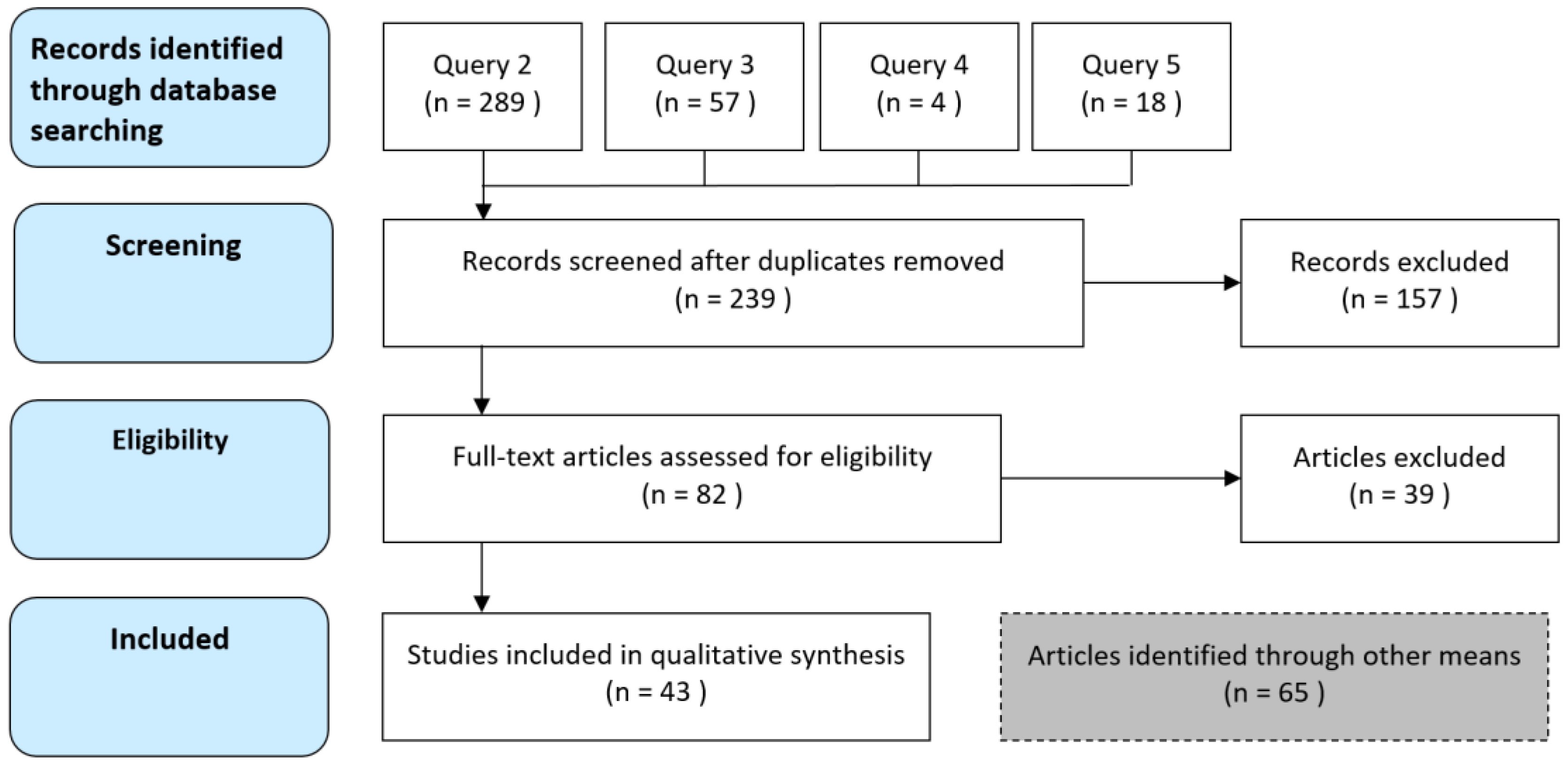
2. Methodology
- ((“Dynamic” AND (“life cycle assessment” OR “lca” or “life cycle analysis”)) OR “DLCA”)
- (1.) AND (“building” or “construction”)
- (1.) AND (“biogenic” or “forest”) AND “carbon”
- (1.) AND “biomaterials”
- (1.) AND (“building” or “construction”) AND (“biogenic” or “forest”) AND “carbon”.
3. Critical Review of the Literature
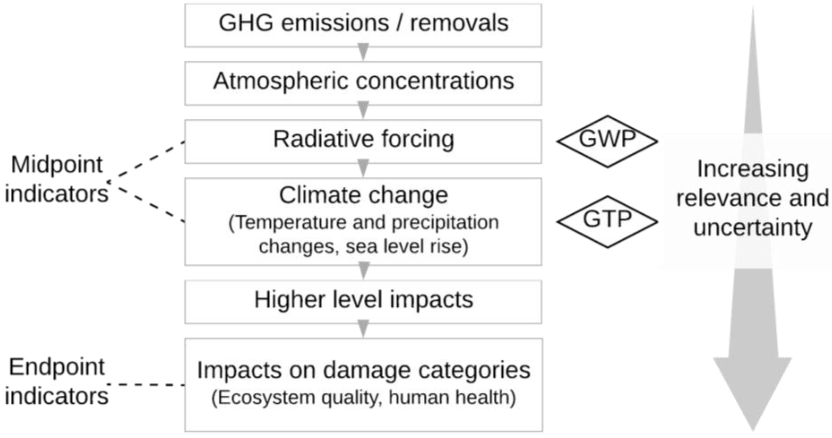
3.1. Conventional LCIA Metrics for Climate Change
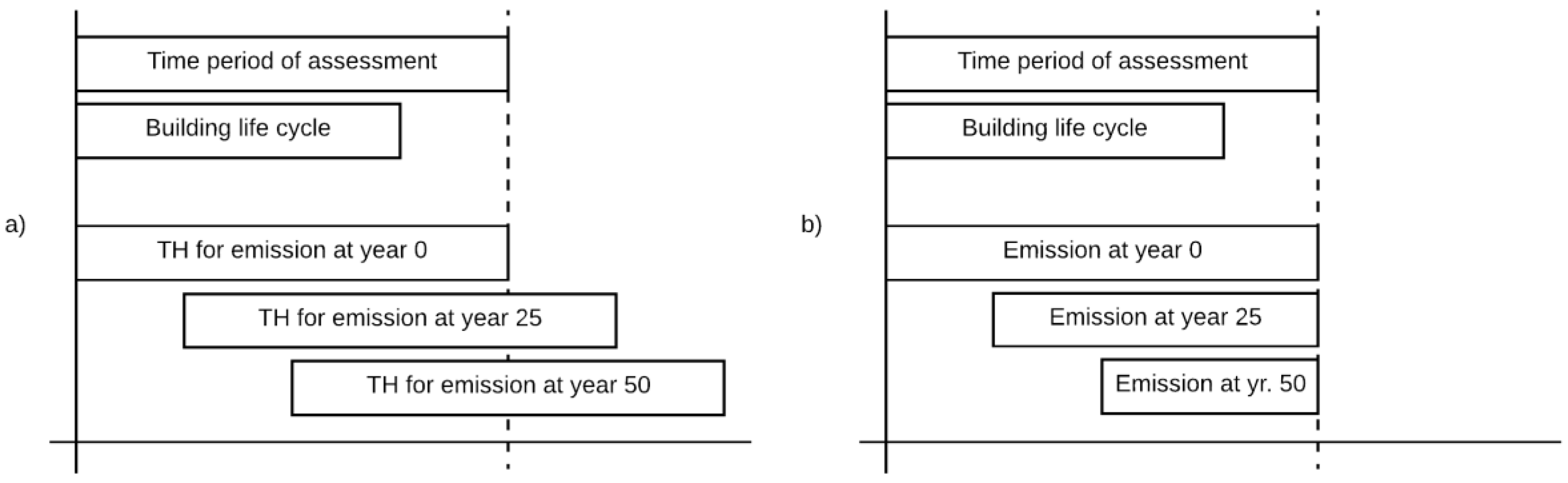
3.2. Time in Conventional LCIA Practice
3.3. Approaches to Include Time in The LCIA of Biogenic Carbon
- Biogenic carbon assessment requires a better understanding of the dynamics of the global carbon cycle;
- The definition of time boundaries for any LCA is highly sensitive and subjective, but temporal issues should be included in the assessment of biogenic carbon;
- For any form of temporary carbon storage, defining assumptions and methodologies clearly and explicitly is important, and both short- and long-term impacts should be considered;
- The use of single metrics (e.g., GWP100) is insufficient, as only the combination of multiple indicators can express the full scale of global warming impacts (cumulative and instantaneous climate effects). No preference was given to having either three mid-point metrics (for impacts i–iii) or a single, aggregated end-point metric.
4. Comparing Two Biogenic Carbon LCIA Methods
4.1. The Dynamic Life Cycle Assessment (DLCA) Framework
4.2. GWPbio, a Metric-Based Alternative to DLCA
A Note on Potential Inconsistencies When Using GWPbio
4.3. Comparison of Both Dynamic Approaches
4.4. Implications for Current Building LCA Practice
5. Limits of This Review
6. Conclusions
Author Contributions
Acknowledgments
Conflicts of Interest
References
- Rockström, J.; Gaffney, O.; Rogelj, J.; Meinshausen, M.; Nakicenovic, N.; Schellnhuber, H.J. A roadmap for rapid decarbonization. Science 2017, 355, 1269–1271. [Google Scholar] [CrossRef] [PubMed] [Green Version]
- UNEP; SBCI. Buildings and Climate Change: A Summary for Decision-Makers; United Nations Environment Programme: Paris, France, 2009. [Google Scholar]
- Levine, M.; Ürge-Vorsatz, D.; Blok, K.; Geng, L.; Harvey, D.; Lang, S.; Levermore, G.; Mongameli Mehlwana, A.; Mirasgedis, S.; Novikova, A.; et al. Residential and commercial buildings. In Climate Change 2007: Mitigation. Contribution of Working Group III to the Fourth Assessment Report of the Intergovernmental Panel on Climate Change; Metz, B., Davidson, O.R., Bosch, P.R., Dave, R., Meyer, L.A., Eds.; Cambridge University Press: Cambridge, UK; New York, NY, USA, 2007; Chapter 6; pp. 387–446. ISBN 9780521880091. [Google Scholar]
- Lucon, O.; Ürge-Vorsatz, D.; Zain Ahmed, A.; Akbari, H.; Bertoldi, P.; Cabeza, L.F.; Eyre, N.; Gadgil, A.; Harvey, L.D.D.; Jiang, Y.; et al. Buildings. In Climate Change 2014: Mitigation of Climate Change: Contribution of Working Group III to the Fifth Assessment Report of the Intergovernmental Panel on Climate Change; Edenhofer, O., Pichs-Madruga, R., Sokona, Y., Farahani, E., Kadner, S., Seyboth, K., Adler, A., Baum, I., Brunner, S., Eickemeier, P., et al., Eds.; Cambridge University Press: Cambridge, UK; New York, NY, USA, 2014; Chapter 9; pp. 671–738. [Google Scholar]
- De Wolf, C.; Pomponi, F.; Moncaster, A. Measuring embodied carbon dioxide equivalent of buildings: A review and critique of current industry practice. Energy Build. 2017, 140, 68–80. [Google Scholar] [CrossRef]
- Moncaster, A.M.; Symons, K.E. A method and tool for ‘cradle to grave’ embodied carbon and energy impacts of UK buildings in compliance with the new TC350 standards. Energy Build. 2013, 66, 514–523. [Google Scholar] [CrossRef]
- Dixit, M.K.; Fernández-Solís, J.L.; Lavy, S.; Culp, C.H. Identification of parameters for embodied energy measurement: A literature review. Energy Build. 2010, 42, 1238–1247. [Google Scholar] [CrossRef]
- Ibn-Mohammed, T.; Greenough, R.; Taylor, S.; Ozawa-Meida, L.; Acquaye, A. Operational vs. embodied emissions in buildings—A review of current trends. Energy Build. 2013, 66, 232–245. [Google Scholar] [CrossRef]
- Rouleau, J.; Gosselin, L.; Blanchet, P. Understanding energy consumption in high-performance social housing buildings: A case study from Canada. Energy 2018, 145, 677–690. [Google Scholar] [CrossRef]
- Cole, R.J.; Kernan, P.C. Life-cycle energy use in office buildings. Build. Environ. 1996, 31, 307–317. [Google Scholar] [CrossRef]
- Sartori, I.; Hestnes, A.G. Energy use in the life cycle of conventional and low-energy buildings: A review article. Energy Build. 2007, 39, 249–257. [Google Scholar] [CrossRef]
- Ramesh, T.; Prakash, R.; Shukla, K.K. Life cycle energy analysis of buildings: An overview. Energy Build. 2010, 42, 1592–1600. [Google Scholar] [CrossRef]
- Anand, C.K.; Amor, B. Recent developments, future challenges and new research directions in LCA of buildings: A critical review. Renew. Sustain. Energy Rev. 2017, 67, 408–416. [Google Scholar] [CrossRef] [Green Version]
- Lessard, Y.; Anand, C.K.; Blanchet, P.; Frenette, C.; Amor, B. LEED v4: Where Are We Now? Critical Assessment through the LCA of an Office Building Using a Low Impact Energy Consumption Mix. J. Ind. Ecol. 2017. [Google Scholar] [CrossRef]
- Fouquet, M.; Levasseur, A.; Margni, M.; Lebert, A.; Lasvaux, S.; Souyri, B.; Buhé, C.; Woloszyn, M. Methodological challenges and developments in LCA of low energy buildings: Application to biogenic carbon and global warming assessment. Build. Environ. 2015, 90, 51–59. [Google Scholar] [CrossRef]
- Ciais, P.; Sabine, C.; Bala, G.; Bopp, L.; Brovkin, V.; Canadell, J.; Chhabra, A.; DeFries, R.; Galloway, J.; Heimann, M.; et al. Carbon and Other Biogeochemical Cycles. In Climate Change 2013—The Physical Science Basis. Contribution of Working Group I to the Fifth Assessment Report of the Intergovernmental Panel on Climate Change; Stocker, T.F., Qin, D., Plattner, G.-K., Tignor, M., Allen, S.K., Boschung, J., Nauels, A., Xia, Y., Bex, V., Midgley, P.M., Eds.; Cambridge University Press: Cambridge, UK; New York, NY, USA, 2013; Chapter 6; pp. 465–570. ISBN 9781107661820. [Google Scholar]
- USGBC. LEED v4 for Building Design and Construction; U.S. Green Building Council: Washington, DC, USA, 2018. [Google Scholar]
- Skullestad, J.L.; Bohne, R.A.; Lohne, J. High-rise Timber Buildings as a Climate Change Mitigation Measure—A Comparative LCA of Structural System Alternatives. Energy Procedia 2016, 96, 112–123. [Google Scholar] [CrossRef]
- Lenzen, M.; Treloar, G. Embodied energy in buildings: Wood versus concrete—Reply to Börjesson and Gustavsson. Energy Policy 2002, 30, 249–255. [Google Scholar] [CrossRef]
- Dodoo, A.; Gustavsson, L.; Sathre, R. Lifecycle carbon implications of conventional and low-energy multi-storey timber building systems. Energy Build. 2014, 82, 194–210. [Google Scholar] [CrossRef]
- Bejo, L. Operational vs. Embodied Energy: A Case for Wood Construction. Drv. Ind. 2017, 68, 163–172. [Google Scholar] [CrossRef]
- Gustavsson, L.; Pingoud, K.; Sathre, R. Carbon Dioxide Balance of Wood Substitution: Comparing Concrete- and Wood-Framed Buildings. Mitig. Adapt. Strateg. Glob. Chang. 2006, 11, 667–691. [Google Scholar] [CrossRef]
- Pan, Y.; Birdsey, R.A.; Fang, J.; Houghton, R.; Kauppi, P.E.; Kurz, W.A.; Phillips, O.L.; Shvidenko, A.; Lewis, S.L.; Canadell, J.G.; et al. A Large and Persistent Carbon Sink in the World’s Forests. Science 2011, 333, 988–993. [Google Scholar] [CrossRef] [PubMed]
- Seidl, R.; Thom, D.; Kautz, M.; Martin-Benito, D.; Peltoniemi, M.; Vacchiano, G.; Wild, J.; Ascoli, D.; Petr, M.; Honkaniemi, J.; et al. Forest disturbances under climate change. Nat. Clim. Chang. 2017, 7, 395–402. [Google Scholar] [CrossRef] [PubMed] [Green Version]
- Kurz, W.A.; Shaw, C.H.; Boisvenue, C.; Stinson, G.; Metsaranta, J.; Leckie, D.; Dyk, A.; Smyth, C.E.; Neilson, E.T. Carbon in Canada’s boreal forest—A synthesis. Environ. Rev. 2013, 21, 260–292. [Google Scholar] [CrossRef]
- Nabuurs, G.J.; Masera, O.; Andrasko, K.; Benitez-Ponce, P.; Boer, R.; Dutschke, M.; Elsiddig, E.A.; Ford-Robertson, J.; Frumhoff, P.; Karjalainen, T.; et al. Forestry. In Climate Change 2007: Mitigation. Contribution of Working Group III to the Fourth Assessment Report of the Intergovernmental Panel on Climate Change; Metz, B., Davidson, O.R., Bosch, P.R., Dave, R., Meyer, L.A., Eds.; Cambridge University Press: Cambridge, UK; New York, NY, USA, 2007; Chapter 9; pp. 541–584. ISBN 0521880114. [Google Scholar]
- Smyth, C.E.; Stinson, G.; Neilson, E.; Lemprière, T.C.; Hafer, M.; Rampley, G.J.; Kurz, W.A. Quantifying the biophysical climate change mitigation potential of Canada’s forest sector. Biogeosciences 2014, 11, 3515–3529. [Google Scholar] [CrossRef]
- Giesekam, J.; Pomponi, F. Briefing: Embodied carbon dioxide assessment in buildings: Guidance and gaps. Proc. Inst. Civ. Eng. Eng. Sustain. 2017, 1–8. [Google Scholar] [CrossRef]
- Gasser, T.; Guivarch, C.; Tachiiri, K.; Jones, C.D.; Ciais, P. Negative emissions physically needed to keep global warming below 2 °C. Nat. Commun. 2015, 6, 7958. [Google Scholar] [CrossRef] [PubMed] [Green Version]
- Lemprière, T.C.; Kurz, W.A.; Hogg, E.H.; Schmoll, C.; Rampley, G.J.; Yemshanov, D.; McKenney, D.W.; Gilsenan, R.; Beatch, A.; Blain, D.; et al. Canadian boreal forests and climate change mitigation. Environ. Rev. 2013, 21, 293–321. [Google Scholar] [CrossRef]
- Thormark, C. The effect of material choice on the total energy need and recycling potential of a building. Build. Environ. 2006, 41, 1019–1026. [Google Scholar] [CrossRef]
- Pajchrowski, G.; Noskowiak, A.; Lewandowska, A.; Strykowski, W. Wood as a building material in the light of environmental assessment of full life cycle of four buildings. Constr. Build. Mater. 2014, 52, 428–436. [Google Scholar] [CrossRef]
- Fava, J.A. Will the Next 10 Years be as Productive in Advancing Life Cycle Approaches as the Last 15 Years? Int. J. Life Cycle Assess. 2006, 11, 6–8. [Google Scholar] [CrossRef]
- McManus, M.C.; Taylor, C.M. The changing nature of life cycle assessment. Biomass Bioenergy 2015, 82, 13–26. [Google Scholar] [CrossRef] [PubMed] [Green Version]
- Guinée, J.B.; Heijungs, R.; Huppes, G.; Zamagni, A.; Masoni, P.; Buonamici, R.; Ekvall, T.; Rydberg, T. Life Cycle Assessment: Past, Present, and Future. Environ. Sci. Technol. 2011, 45, 90–96. [Google Scholar] [CrossRef] [PubMed]
- Hellweg, S.; Mila i Canals, L. Emerging approaches, challenges and opportunities in life cycle assessment. Science 2014, 344, 1109–1113. [Google Scholar] [CrossRef] [PubMed]
- De Rosa, M.; Schmidt, J.; Brandão, M.; Pizzol, M. A flexible parametric model for a balanced account of forest carbon fluxes in LCA. Int. J. Life Cycle Assess. 2017, 22, 172–184. [Google Scholar] [CrossRef]
- Helin, T.; Sokka, L.; Soimakallio, S.; Pingoud, K.; Pajula, T. Approaches for inclusion of forest carbon cycle in life cycle assessment—A review. GCB Bioenergy 2013, 5, 475–486. [Google Scholar] [CrossRef]
- Guinée, J.B.; Heijungs, R.; van der Voet, E. A greenhouse gas indicator for bioenergy: Some theoretical issues with practical implications. Int. J. Life Cycle Assess. 2009, 14, 328–339. [Google Scholar] [CrossRef]
- Levasseur, A.; Lesage, P.; Margni, M.; Deschênes, L.; Samson, R. Considering Time in LCA: Dynamic LCA and Its Application to Global Warming Impact Assessments. Environ. Sci. Technol. 2010, 44, 3169–3174. [Google Scholar] [CrossRef] [PubMed]
- Collinge, W.O.; Landis, A.E.; Jones, A.K.; Schaefer, L.A.; Bilec, M.M. Dynamic life cycle assessment: Framework and application to an institutional building. Int. J. Life Cycle Assess. 2013, 18, 538–552. [Google Scholar] [CrossRef]
- Su, S.; Li, X.; Zhu, Y.; Lin, B. Dynamic LCA framework for environmental impact assessment of buildings. Energy Build. 2017, 149, 310–320. [Google Scholar] [CrossRef]
- Buyle, M.; Braet, J.; Audenaert, A. Life Cycle Assessment of an Apartment Building: Comparison of an Attributional and Consequential Approach. Energy Procedia 2014, 62, 132–140. [Google Scholar] [CrossRef]
- Suh, S.; Huppes, G. Methods for life cycle inventory of a product. J. Clean. Prod. 2005, 13, 687–697. [Google Scholar] [CrossRef]
- Brander, M.; Tipper, R.; Hutchison, C.; Davis, G. Consequential and Attributional Approaches to LCA: A Guide to Policy Makers with Specific Reference to Greenhouse Gas LCA of Biofuels; Ecometrica Press: Edinburgh, UK, 2008; Volume 44. [Google Scholar]
- Grant, M.J.; Booth, A. A typology of reviews: An analysis of 14 review types and associated methodologies. Health Inf. Libr. J. 2009, 26, 91–108. [Google Scholar] [CrossRef] [PubMed]
- Nelson, J. Using conceptual depth criteria: Addressing the challenge of reaching saturation in qualitative research. Qual. Res. 2016, 69–71. [Google Scholar] [CrossRef]
- Booth, A. Unpacking your literature search toolbox: On search styles and tactics. Health Inf. Libr. J. 2008, 25, 313–317. [Google Scholar] [CrossRef] [PubMed]
- Mason, M. Sample Size and Saturation in PhD Studies Using Qualitative Interviews. Forum Qual. Sozialforsch. Forum Qual. Soc. Res. 2010, 11. [Google Scholar] [CrossRef]
- O’Reilly, M.; Parker, N. ‘Unsatisfactory Saturation’: A critical exploration of the notion of saturated sample sizes in qualitative research. Qual. Res. 2013, 13, 190–197. [Google Scholar] [CrossRef]
- Moher, D.; Liberati, A.; Tetzlaff, J.; Altman, D.G. Preferred Reporting Items for Systematic Reviews and Meta-Analyses: The PRISMA Statement. PLoS Med. 2009, 6, e1000097. [Google Scholar] [CrossRef] [PubMed]
- Brandão, M.; Levasseur, A.; Kirschbaum, M.U.F.; Weidema, B.P.; Cowie, A.L.; Jørgensen, S.V.; Hauschild, M.Z.; Pennington, D.W.; Chomkhamsri, K. Key issues and options in accounting for carbon sequestration and temporary storage in life cycle assessment and carbon footprinting. Int. J. Life Cycle Assess. 2013, 18, 230–240. [Google Scholar] [CrossRef]
- Brandão, M.; Levasseur, A. Assessing Temporary Carbon Storage in Life Cycle Assessment and Carbon Footprinting: Outcomes of an Expert Workshop; Publications Office of the European Union: Luxembourg, 2011. [Google Scholar]
- Levasseur, A.; Cavalett, O.; Fuglestvedt, J.S.; Gasser, T.; Johansson, D.J.A.; Jørgensen, S.V.; Raugei, M.; Reisinger, A.; Schivley, G.; Strømman, A.; et al. Enhancing life cycle impact assessment from climate science: Review of recent findings and recommendations for application to LCA. Ecol. Indic. 2016, 71, 163–174. [Google Scholar] [CrossRef]
- Levasseur, A. Climate Change. In Life Cycle Impact Assessment; Hauschild, M.Z., Huijbregts, M.A.J., Eds.; LCA Compendium—The Complete World of Life Cycle Assessment; Springer: Dordrecht, The Netherlands, 2015; pp. 39–50. ISBN 978-94-017-9743-6. [Google Scholar]
- Cherubini, F.; Fuglestvedt, J.S.; Gasser, T.; Reisinger, A.; Cavalett, O.; Huijbregts, M.A.J.; Johansson, D.J.A.; Jørgensen, S.V.; Raugei, M.; Schivley, G.; et al. Bridging the gap between impact assessment methods and climate science. Environ. Sci. Policy 2016, 64, 129–140. [Google Scholar] [CrossRef]
- Pawelzik, P.; Carus, M.; Hotchkiss, J.; Narayan, R.; Selke, S.; Wellisch, M.; Weiss, M.; Wicke, B.; Patel, M.K. Critical aspects in the life cycle assessment (LCA) of bio-based materials—Reviewing methodologies and deriving recommendations. Resour. Conserv. Recycl. 2013, 73, 211–228. [Google Scholar] [CrossRef]
- Brown, S.; Lim, B.; Schlamadinger, B. Evaluating approaches for estimating net emissions of carbon dioxide from forest harvesting and wood products. In Proceedings of the IPCC/OECD/IEA Programme on National Greenhouse Gas Inventories, Dakar, Senegal, 5–7 May 1998; Intergovernmental Panel on Climate Change: Geneva, Switzerland, 1998. [Google Scholar]
- Apps, M.J.; Kurz, W.A.; Beukema, S.J.; Bhatti, J.S. Carbon budget of the Canadian forest product sector. Environ. Sci. Policy 1999, 2, 25–41. [Google Scholar] [CrossRef]
- De Rosa, M.; Pizzol, M.; Schmidt, J. How methodological choices affect LCA climate impact results: The case of structural timber. Int. J. Life Cycle Assess. 2018, 23, 147–158. [Google Scholar] [CrossRef]
- Guest, G.; Cherubini, F.; Strømman, A.H. Global Warming Potential of Carbon Dioxide Emissions from Biomass Stored in the Anthroposphere and Used for Bioenergy at End of Life. J. Ind. Ecol. 2013, 17, 20–30. [Google Scholar] [CrossRef]
- Jørgensen, S.V.; Hauschild, M.Z.; Nielsen, P.H. The potential contribution to climate change mitigation from temporary carbon storage in biomaterials. Int. J. Life Cycle Assess. 2015, 20, 451–462. [Google Scholar] [CrossRef] [Green Version]
- Levasseur, A.; Lesage, P.; Margni, M.; Samson, R. Biogenic Carbon and Temporary Storage Addressed with Dynamic Life Cycle Assessment. J. Ind. Ecol. 2013, 17, 117–128. [Google Scholar] [CrossRef]
- Ellison, D.; Lundblad, M.; Petersson, H. Carbon accounting and the climate politics of forestry. Environ. Sci. Policy 2011, 14, 1062–1078. [Google Scholar] [CrossRef]
- Cherubini, F.; Strømman, A.H.; Hertwich, E. Effects of boreal forest management practices on the climate impact of CO2 emissions from bioenergy. Ecol. Model. 2011, 223, 59–66. [Google Scholar] [CrossRef]
- Jolliet, O.; Brent, A.; Goedkoop, M.; Itsubo, N.; Mueller-Wenk, R.; Peña, C.; Schenk, R.; Stewart, M.; Weidema, B.; Bare, J.; et al. Final Report of the LCIA Definition Study; Life Cycle Impact Assessment Programme of the Life Cycle Initiative: Paris, France, 2003. [Google Scholar]
- Cherubini, F.; Bright, R.M.; Strømman, A.H. Global climate impacts of forest bioenergy: What, when and how to measure? Environ. Res. Lett. 2013, 8, 014049. [Google Scholar] [CrossRef]
- Peters, G.P.; Aamaas, B.; Lund, M.T.; Solli, C.; Fuglestvedt, J.S. Alternative “Global Warming” Metrics in Life Cycle Assessment: A Case Study with Existing Transportation Data. Environ. Sci. Technol. 2011, 45, 8633–8641. [Google Scholar] [CrossRef] [PubMed]
- Cherubini, F.; Guest, G.; Strømman, A.H. Application of probability distributions to the modeling of biogenic CO2 fluxes in life cycle assessment. GCB Bioenergy 2012, 4, 784–798. [Google Scholar] [CrossRef]
- Shine, K.P.; Derwent, R.G.; Wuebbles, D.J.; Morcrette, J.-J. Radiative forcing of climate. In Climate Change: The IPCC Scientific Assessment. Report Prepared by Working Group I for Intergovernmental Panel on Climate Change; Houghton, J.T., Jenkins, G.J., Ephraum, J.J., Eds.; Cambridge University Press: Cambridge, UK; New York, NY, USA; Melbourne, Australia, 1990; Chapter 2; pp. 41–68. ISBN 0521407206. [Google Scholar]
- Cherubini, F.; Huijbregts, M.; Kindermann, G.; Van Zelm, R.; Van Der Velde, M.; Stadler, K.; Strømman, A.H. Global spatially explicit CO2 emission metrics for forest bioenergy. Sci. Rep. 2016, 6, 20186. [Google Scholar] [CrossRef] [PubMed] [Green Version]
- Shine, K.P.; Fuglestvedt, J.S.; Hailemariam, K.; Stuber, N. Alternatives to the Global Warming Potential for Comparing Climate Impacts of Emissions of Greenhouse Gases. Clim. Chang. 2005, 68, 281–302. [Google Scholar] [CrossRef] [Green Version]
- Shine, K.P.; Berntsen, T.K.; Fuglestvedt, J.S.; Skeie, R.B.; Stuber, N. Comparing the climate effect of emissions of short- and long-lived climate agents. Philos. Trans. R. Soc. A Math. Phys. Eng. Sci. 2007, 365, 1903–1914. [Google Scholar] [CrossRef] [PubMed] [Green Version]
- Shine, K.P. The global warming potential—The need for an interdisciplinary retrial. Clim. Chang. 2009, 96, 467–472. [Google Scholar] [CrossRef]
- Fuglestvedt, J.S. Metrics of Climate Change: Assessing Radiative Forcing and Emission Indices. Clim. Chang. 2003, 58, 267–331. [Google Scholar] [CrossRef]
- Pierrehumbert, R.T. Short-Lived Climate Pollution. Annu. Rev. Earth Planet. Sci. 2014, 42, 341–379. [Google Scholar] [CrossRef]
- Smith, S.J.; Wigley, T.M.L. Global Warming Potentials: 2. Accuracy. Clim. Chang. 2000, 44, 459–469. [Google Scholar] [CrossRef]
- Cherubini, F.; Tanaka, K. Amending the Inadequacy of a Single Indicator for Climate Impact Analyses. Environ. Sci. Technol. 2016, 50, 12530–12531. [Google Scholar] [CrossRef] [PubMed]
- Allen, M.R.; Fuglestvedt, J.S.; Shine, K.P.; Reisinger, A.; Pierrehumbert, R.T.; Forster, P.M. New use of global warming potentials to compare cumulative and short-lived climate pollutants. Nat. Clim. Chang. 2016, 6, 773–776. [Google Scholar] [CrossRef] [Green Version]
- Jolliet, O.; Antón, A.; Boulay, A.-M.; Cherubini, F.; Fantke, P.; Levasseur, A.; McKone, T.E.; Michelsen, O.; Milà i Canals, L.; Motoshita, M.; et al. Global guidance on environmental life cycle impact assessment indicators: Impacts of climate change, fine particulate matter formation, water consumption and land use. Int. J. Life Cycle Assess. 2018, 1–19. [Google Scholar] [CrossRef]
- Myhre, G.; Shindell, D.; Bréon, F.-M.F.-M.; Collins, W.; Fuglestvedt, J.S.; Huang, J.; Koch, D.; Lamarque, J.-F.J.-F.; Lee, D.; Mendoza, B.; et al. Anthropogenic and Natural Radiative Forcing—Supplementary Material. In Climate Change 2013: The Physical Science Basis. Contribution of Working Group I to the Fifth Assessment Report of the Intergovernmental Panel on Climate Change; UNEP: Nairobi, Kenya, 2013; Chapter 8SM; pp. 1–44. [Google Scholar]
- Moura-Costa, P.; Wilson, C. An Equivalence Factor between CO2 Avoided Emissions and Sequestration—Description and Applications in Forestry. Mitig. Adapt. Strateg. Glob. Chang. 2000, 5, 51–60. [Google Scholar] [CrossRef]
- Fearnside, P.M.; Lashof, D.A.; Moura-Costa, P. Accounting for time in mitigating global warming through land-use change and forestry. Mitig. Adapt. Strateg. Glob. Chang. 2000, 5, 239–270. [Google Scholar] [CrossRef]
- Clift, R.; Brandão, M. Carbon Storage and Timing of Emissions—A Note by Roland Clift and Miguel Brandao; Centre for Environmental Strategy, University of Surrey: Surrey, UK, 2008. [Google Scholar]
- Marland, G.; Marland, E.S.; Shirley, K.; Cantrell, J.; Stellar, K. Accounting for sequestered carbon: The value of temporary storage. In Assessing Temporary Carbon Storage in Life Cycle Assessment and Carbon Footprinting: Outcomes of an Expert Workshop; Publications Office of the European Union: Luxembourg, 2011; pp. 51–53. [Google Scholar]
- Marland, G.H.; Marland, E.S. Trading permanent and temporary carbon emissions credits. Clim. Chang. 2009, 95, 465–468. [Google Scholar] [CrossRef]
- Kirschbaum, M.U.F. To sink or burn? A discussion of the potential contributions of forests to greenhouse gas balances through storing carbon or providing biofuels. Biomass Bioenergy 2003, 24, 297–310. [Google Scholar] [CrossRef]
- Kirschbaum, M.U.F. Can Trees Buy Time? An Assessment of the Role of Vegetation Sinks as Part of the Global Carbon Cycle. Clim. Chang. 2003, 58, 47–71. [Google Scholar] [CrossRef]
- Kirschbaum, M.U.F. Temporary Carbon Sequestration Cannot Prevent Climate Change. Mitig. Adapt. Strateg. Glob. Chang. 2006, 11, 1151–1164. [Google Scholar] [CrossRef]
- Kirschbaum, M.U.F. Temporary Carbon Sequestration Cannot Prevent Climate Change. In Assessing Temporary Carbon Storage in Life Cycle Assessment and Carbon Footprinting: Outcomes of an Expert Workshop; Publications Office of the European Union: Luxembourg, 2011; pp. 38–50. [Google Scholar]
- Levasseur, A.; Lesage, P.; Margni, M.; Brandão, M.; Samson, R. Assessing temporary carbon sequestration and storage projects through land use, land-use change and forestry: Comparison of dynamic life cycle assessment with ton-year approaches. Clim. Chang. 2012, 115, 759–776. [Google Scholar] [CrossRef] [Green Version]
- Hansen, J.; Sato, M.; Kharecha, P.; Beerling, D.; Berner, R.; Masson-Delmotte, V.; Pagani, M.; Raymo, M.; Royer, D.L.; Zachos, J.C. Target Atmospheric CO2: Where Should Humanity Aim? Open Atmos. Sci. J. 2008, 2, 217–231. [Google Scholar] [CrossRef]
- Jørgensen, S.V.; Hauschild, M.Z.; Nielsen, P.H. Assessment of urgent impacts of greenhouse gas emissions—The climate tipping potential (CTP). Int. J. Life Cycle Assess. 2014, 19, 919–930. [Google Scholar] [CrossRef]
- Røyne, F.; Peñaloza, D.; Sandin, G.; Berlin, J.; Svanström, M. Climate impact assessment in life cycle assessments of forest products: Implications of method choice for results and decision-making. J. Clean. Prod. 2016, 116, 90–99. [Google Scholar] [CrossRef]
- Tellnes, L.G.F.; Ganne-Chedeville, C.; Dias, A.; Dolezal, F.; Hill, C.; Escamilla, E.Z. Comparative assessment for biogenic carbon accounting methods in carbon footprint of products: A review study for construction materials based on forest products. IForest 2017, 10, 815–823. [Google Scholar] [CrossRef]
- Peñaloza, D.; Erlandsson, M.; Falk, A. Exploring the climate impact effects of increased use of bio-based materials in buildings. Constr. Build. Mater. 2016, 125, 219–226. [Google Scholar] [CrossRef] [Green Version]
- Jørgensen, S.V.; Hauschild, M.Z. Need for relevant timescales when crediting temporary carbon storage. Int. J. Life Cycle Assess. 2013, 18, 747–754. [Google Scholar] [CrossRef]
- Guest, G.; Bright, R.M.; Cherubini, F.; Strømman, A.H. Consistent quantification of climate impacts due to biogenic carbon storage across a range of bio-product systems. Environ. Impact Assess. Rev. 2013, 43, 21–30. [Google Scholar] [CrossRef]
- Suter, F.; Steubing, B.; Hellweg, S. Life Cycle Impacts and Benefits of Wood along the Value Chain: The Case of Switzerland. J. Ind. Ecol. 2017, 21, 874–886. [Google Scholar] [CrossRef]
- Perez-Garcia, J.; Lippke, B.; Comnick, J.; Manriquez, C. An assessment of carbon pools, storage, and wood products market substitution using life-cycle analysis results. Wood Fiber Sci. 2005, 37, 140–148. [Google Scholar]
- Sathre, R.; O’Connor, J. Meta-analysis of greenhouse gas displacement factors of wood product substitution. Environ. Sci. Policy 2010, 13, 104–114. [Google Scholar] [CrossRef]
- Smyth, C.E.; Rampley, G.; Lemprière, T.C.; Schwab, O.; Kurz, W.A. Estimating product and energy substitution benefits in national-scale mitigation analyses for Canada. GCB Bioenergy 2017, 9, 1071–1084. [Google Scholar] [CrossRef]
- Yan, Y. Integrate carbon dynamic models in analyzing carbon sequestration impact of forest biomass harvest. Sci. Total Environ. 2018, 615, 581–587. [Google Scholar] [CrossRef] [PubMed]
- Sterman, J.D.; Siegel, L.; Rooney-Varga, J.N. Does replacing coal with wood lower CO2 emissions? Dynamic lifecycle analysis of wood bioenergy. Environ. Res. Lett. 2018, 13, 015007. [Google Scholar] [CrossRef]
- Boucher, O.; Reddy, M.S. Climate trade-off between black carbon and carbon dioxide emissions. Energy Policy 2008, 36, 193–200. [Google Scholar] [CrossRef]
- Boucher, O.; Friedlingstein, P.; Collins, B.; Shine, K.P. The indirect global warming potential and global temperature change potential due to methane oxidation. Environ. Res. Lett. 2009, 4, 044007. [Google Scholar] [CrossRef] [Green Version]
- Ericsson, N.; Porsö, C.; Ahlgren, S.; Nordberg, Å.; Sundberg, C.; Hansson, P.-A. Time-dependent climate impact of a bioenergy system—Methodology development and application to Swedish conditions. GCB Bioenergy 2013, 5, 580–590. [Google Scholar] [CrossRef]
- Hammar, T.; Ortiz, C.A.; Stendahl, J.; Ahlgren, S.; Hansson, P.-A. Time-Dynamic Effects on the Global Temperature When Harvesting Logging Residues for Bioenergy. BioEnergy Res. 2015, 8, 1912–1924. [Google Scholar] [CrossRef] [Green Version]
- Ortiz, C.A.; Hammar, T.; Ahlgren, S.; Hansson, P.-A.; Stendahl, J. Time-dependent global warming impact of tree stump bioenergy in Sweden. For. Ecol. Manag. 2016, 371, 5–14. [Google Scholar] [CrossRef]
- Aracil, C.; Haro, P.; Giuntoli, J.; Ollero, P. Proving the climate benefit in the production of biofuels from municipal solid waste refuse in Europe. J. Clean. Prod. 2017, 142, 2887–2900. [Google Scholar] [CrossRef]
- Kilpeläinen, A.; Kellomäki, S.; Strandman, H. Net atmospheric impacts of forest bioenergy production and utilization in Finnish boreal conditions. GCB Bioenergy 2012, 4, 811–817. [Google Scholar] [CrossRef] [Green Version]
- Haus, S.; Gustavsson, L.; Sathre, R. Climate mitigation comparison of woody biomass systems with the inclusion of land-use in the reference fossil system. Biomass Bioenergy 2014, 65, 136–144. [Google Scholar] [CrossRef]
- Sathre, R.; Gustavsson, L. Time-dependent radiative forcing effects of forest fertilization and biomass substitution. Biogeochemistry 2012, 109, 203–218. [Google Scholar] [CrossRef]
- Giuntoli, J.; Caserini, S.; Marelli, L.; Baxter, D.; Agostini, A. Domestic heating from forest logging residues: Environmental risks and benefits. J. Clean. Prod. 2015, 99, 206–216. [Google Scholar] [CrossRef] [Green Version]
- Giuntoli, J.; Agostini, A.; Caserini, S.; Lugato, E.; Baxter, D.; Marelli, L. Climate change impacts of power generation from residual biomass. Biomass Bioenergy 2016, 89, 146–158. [Google Scholar] [CrossRef]
- Kendall, A. Time-adjusted global warming potentials for LCA and carbon footprints. Int. J. Life Cycle Assess. 2012, 17, 1042–1049. [Google Scholar] [CrossRef]
- Petersen, A.K.; Solberg, B. Greenhouse Gas Emissions and Costs over the Life Cycle of Wood and Alternative Flooring Materials. Clim. Chang. 2004, 64, 143–167. [Google Scholar] [CrossRef]
- Petersen, A.K.; Solberg, B. Greenhouse gas emissions, life-cycle inventory and cost-efficiency of using laminated wood instead of steel construction. Environ. Sci. Policy 2002, 5, 169–182. [Google Scholar] [CrossRef]
- Kirkinen, J.; Palosuo, T.; Holmgren, K.; Savolainen, I. Greenhouse Impact Due to the Use of Combustible Fuels: Life Cycle Viewpoint and Relative Radiative Forcing Commitment. Environ. Manag. 2008, 42, 458–469. [Google Scholar] [CrossRef] [PubMed] [Green Version]
- Kirkinen, J. Greenhouse Impact Assessment of Some Combustible Fuels with a Dynamic Life Cycle Approach; VTT Publications: Espoo, Finland, 2010. [Google Scholar]
- O’Hare, M.; Plevin, R.J.; Martin, J.I.; Jones, A.D.; Kendall, A.; Hopson, E. Proper accounting for time increases crop-based biofuels’ greenhouse gas deficit versus petroleum. Environ. Res. Lett. 2009, 4, 024001. [Google Scholar] [CrossRef] [Green Version]
- Kendall, A.; Price, L. Incorporating Time-Corrected Life Cycle Greenhouse Gas Emissions in Vehicle Regulations. Environ. Sci. Technol. 2012, 46, 2557–2563. [Google Scholar] [CrossRef] [PubMed]
- Kendall, A.; Chang, B.; Sharpe, B. Accounting for Time-Dependent Effects in Biofuel Life Cycle Greenhouse Gas Emissions Calculations. Environ. Sci. Technol. 2009, 43, 7142–7147. [Google Scholar] [CrossRef] [PubMed]
- Collinge, W.O.; Liao, L.; Xu, H.; Saunders, C.L.; Bilec, M.M.; Landis, A.E.; Jones, A.K.; Schaefer, L.A. Enabling dynamic life cycle assessment of buildings with wireless sensor networks. In Proceedings of the 2011 IEEE International Symposium on Sustainable Systems and Technology (ISSST), Chicago, IL, USA, 16–18 May 2011; pp. 1–6. [Google Scholar]
- Cherubini, F.; Peters, G.P.; Berntsen, T.; Strømman, A.H.; Hertwich, E. CO2 emissions from biomass combustion for bioenergy: Atmospheric decay and contribution to global warming. GCB Bioenergy 2011, 3, 413–426. [Google Scholar] [CrossRef]
- Peñaloza, D.; Erlandsson, M.; Pousette, A. Climate impacts from road bridges: Effects of introducing concrete carbonation and biogenic carbon storage in wood. Struct. Infrastruct. Eng. 2018, 14, 56–67. [Google Scholar] [CrossRef]
- Almeida, J.; Degerickx, J.; Achten, W.M.J.; Muys, B. Greenhouse gas emission timing in life cycle assessment and the global warming potential of perennial energy crops. Carbon Manag. 2015, 6, 185–195. [Google Scholar] [CrossRef]
- Pittau, F.; Krause, F.; Lumia, G.; Habert, G. Fast-growing bio-based materials as an opportunity for storing carbon in exterior walls. Build. Environ. 2018, 129, 117–129. [Google Scholar] [CrossRef]
- Gaudreault, C.; Miner, R. Temporal Aspects in Evaluating the Greenhouse Gas Mitigation Benefits of Using Residues from Forest Products Manufacturing Facilities for Energy Production. J. Ind. Ecol. 2015, 19, 994–1007. [Google Scholar] [CrossRef]
- Yang, J.; Chen, B. Global warming impact assessment of a crop residue gasification project—A dynamic LCA perspective. Appl. Energy 2014, 122, 269–279. [Google Scholar] [CrossRef]
- Beloin-Saint-Pierre, D.; Heijungs, R.; Blanc, I. The ESPA (Enhanced Structural Path Analysis) method: A solution to an implementation challenge for dynamic life cycle assessment studies. Int. J. Life Cycle Assess. 2014, 19, 861–871. [Google Scholar] [CrossRef] [Green Version]
- Beloin-Saint-Pierre, D.; Levasseur, A.; Margni, M.; Blanc, I. Implementing a Dynamic Life Cycle Assessment Methodology with a Case Study on Domestic Hot Water Production. J. Ind. Ecol. 2017, 21, 1128–1138. [Google Scholar] [CrossRef]
- Dyckhoff, H.; Kasah, T. Time Horizon and Dominance in Dynamic Life Cycle Assessment. J. Ind. Ecol. 2014, 18, 799–808. [Google Scholar] [CrossRef]
- Pinsonnault, A.; Lesage, P.; Levasseur, A.; Samson, R. Temporal differentiation of background systems in LCA: Relevance of adding temporal information in LCI databases. Int. J. Life Cycle Assess. 2014, 19, 1843–1853. [Google Scholar] [CrossRef]
- Bright, R.M.; Cherubini, F.; Strømman, A.H. Climate impacts of bioenergy: Inclusion of carbon cycle and albedo dynamics in life cycle impact assessment. Environ. Impact Assess. Rev. 2012, 37, 2–11. [Google Scholar] [CrossRef]
- Guest, G.; Strømman, A.H. Climate Change Impacts Due to Biogenic Carbon: Addressing the Issue of Attribution Using Two Metrics with Very Different Outcomes. J. Sustain. For. 2014, 33, 298–326. [Google Scholar] [CrossRef]
- Mehr, J.; Vadenbo, C.; Steubing, B.; Hellweg, S. Environmentally optimal wood use in Switzerland—Investigating the relevance of material cascades. Resour. Conserv. Recycl. 2018, 131, 181–191. [Google Scholar] [CrossRef]
- Cherubini, F.; Bright, R.M.; Strømman, A.H. Site-specific global warming potentials of biogenic CO2 for bioenergy: Contributions from carbon fluxes and albedo dynamics. Environ. Res. Lett. 2012, 7, 045902. [Google Scholar] [CrossRef]
- Cherubini, F.; Guest, G.; Strømman, A.H. Bioenergy from forestry and changes in atmospheric CO2: Reconciling single stand and landscape level approaches. J. Environ. Manag. 2013, 129, 292–301. [Google Scholar] [CrossRef] [PubMed]
- Collinge, W.O.; Landis, A.E.; Jones, A.K.; Schaefer, L.A.; Bilec, M.M. Indoor environmental quality in a dynamic life cycle assessment framework for whole buildings: Focus on human health chemical impacts. Build. Environ. 2013, 62, 182–190. [Google Scholar] [CrossRef]
- Collinge, W.O.; Landis, A.E.; Jones, A.K.; Schaefer, L.A.; Bilec, M.M. Productivity metrics in dynamic LCA for whole buildings: Using a post-occupancy evaluation of energy and indoor environmental quality tradeoffs. Build. Environ. 2014, 82, 339–348. [Google Scholar] [CrossRef]
- Pingoud, K.; Ekholm, T.; Savolainen, I. Global warming potential factors and warming payback time as climate indicators of forest biomass use. Mitig. Adapt. Strateg. Glob. Chang. 2012, 17, 369–386. [Google Scholar] [CrossRef]
- Holtsmark, B. Boreal forest management and its effect on atmospheric CO2. Ecol. Model. 2013, 248, 130–134. [Google Scholar] [CrossRef]
- Helin, T.; Salminen, H.; Hynynen, J.; Soimakallio, S.; Huuskonen, S.; Pingoud, K. Global warming potentials of stemwood used for energy and materials in Southern Finland: Differentiation of impacts based on type of harvest and product lifetime. GCB Bioenergy 2016, 8, 334–345. [Google Scholar] [CrossRef]
- Joos, F.; Roth, R.; Fuglestvedt, J.S.; Peters, G.P.; Enting, I.G.; von Bloh, W.; Brovkin, V.; Burke, E.J.; Eby, M.; Edwards, N.R.; et al. Carbon dioxide and climate impulse response functions for the computation of greenhouse gas metrics: A multi-model analysis. Atmos. Chem. Phys. 2013, 13, 2793–2825. [Google Scholar] [CrossRef] [Green Version]
- Olivié, D.J.L.; Peters, G.P. Variation in emission metrics due to variation in CO2 and temperature impulse response functions. Earth Syst. Dyn. 2013, 4, 267–286. [Google Scholar] [CrossRef]
- Huijbregts, M.A.J. A critical view on scientific consensus building in life cycle impact assessment. Int. J. Life Cycle Assess. 2014, 19, 477–479. [Google Scholar] [CrossRef]
- Tellnes, L.G.F.; Gobakken, L.R.; Flæte, P.O.; Alfredsen, G. Carbon footprint including effect of carbon storage for selected wooden facade materials. Wood Mater. Sci. Eng. 2014, 9, 139–143. [Google Scholar] [CrossRef]
- Cherubini, F.; Strømman, A.H.; Hertwich, E. Biogenic CO2 fluxes from bioenergy and climate—A response. Ecol. Model. 2013, 253, 79–81. [Google Scholar] [CrossRef]
- Wigley, T.M.L. A simple inverse carbon cycle model. Glob. Biogeochem. Cycles 1991, 5, 373–382. [Google Scholar] [CrossRef]
- Joos, F.; Bruno, M.; Fink, R.; Siegenthaler, U.; Stocker, T.F.; Le Quéré, C.; Sarmiento, J.L. An efficient and accurate representation of complex oceanic and biospheric models of anthropogenic carbon uptake. Tellus B 1996, 48, 397–417. [Google Scholar] [CrossRef]
- Maier-Reimer, E.; Hasselmann, K. Transport and storage of CO2 in the ocean—An inorganic ocean—Circulation carbon cycle model. Clim. Dyn. 1987, 2, 63–90. [Google Scholar] [CrossRef]
- Schnute, J. A Versatile Growth Model with Statistically Stable Parameters. Can. J. Fish. Aquat. Sci. 1981, 38, 1128–1140. [Google Scholar] [CrossRef]
- Liu, Z.; Li, F. The generalized Chapman-Richards function and applications to tree and stand growth. J. For. Res. 2003, 14, 19–26. [Google Scholar] [CrossRef]
- Marland, E.S.; Stellar, K.; Marland, G.H. A distributed approach to accounting for carbon in wood products. Mitig. Adapt. Strateg. Glob. Chang. 2010, 15, 71–91. [Google Scholar] [CrossRef]
- KT Innovations; Thinkstep; Autodesk Tally—OVERVIEW. Available online: http://choosetally.com/overview (accessed on 2 April 2018).
- UBUBI—The Cloud-Powered LCA Tool for Sustainable Buildings. Available online: http://www.ububi.org/papers.html (accessed on 2 April 2018).
- Dupuis, M.; April, A.; Lesage, P.; Forgues, D. Method to Enable LCA Analysis through Each Level of Development of a BIM Model. Procedia Eng. 2017, 196, 857–863. [Google Scholar] [CrossRef]
- Hollberg, A.; Ruth, J. LCA in architectural design—A parametric approach. Int. J. Life Cycle Assess. 2016, 21, 943–960. [Google Scholar] [CrossRef]
- Lolli, N.; Fufa, S.M.; Inman, M. A Parametric Tool for the Assessment of Operational Energy Use, Embodied Energy and Embodied Material Emissions in Building. Energy Procedia 2017, 111, 21–30. [Google Scholar] [CrossRef]
- Pauliuk, S.; Majeau-Bettez, G.; Mutel, C.L.; Steubing, B.; Stadler, K. Lifting Industrial Ecology Modeling to a New Level of Quality and Transparency: A Call for More Transparent Publications and a Collaborative Open Source Software Framework. J. Ind. Ecol. 2015, 19, 937–949. [Google Scholar] [CrossRef] [Green Version]
- Steubing, B. Activity Browser—A Free and Extendable LCA Software. Available online: https://bitbucket.org/bsteubing/activity-browser (accessed on 2 April 2018).
- CIRAIG DYNCO2 Dynamic Carbon Footprinter. Available online: http://www.ciraig.org/en/dynco2.php (accessed on 27 March 2018).
- Cabeza, L.F.; Rincón, L.; Vilariño, V.; Pérez, G.; Castell, A. Life cycle assessment (LCA) and life cycle energy analysis (LCEA) of buildings and the building sector: A review. Renew. Sustain. Energy Rev. 2014, 29, 394–416. [Google Scholar] [CrossRef]
- Erlandsson, M.; Borg, M. Generic LCA-methodology applicable for buildings, constructions and operation services—Today practice and development needs. Build. Environ. 2003, 38, 919–938. [Google Scholar] [CrossRef]
- Khasreen, M.; Banfill, P.F.; Menzies, G. Life-Cycle Assessment and the Environmental Impact of Buildings: A Review. Sustainability 2009, 1, 674–701. [Google Scholar] [CrossRef] [Green Version]
- Ortiz, O.; Castells, F.; Sonnemann, G. Sustainability in the construction industry: A review of recent developments based on LCA. Constr. Build. Mater. 2009, 23, 28–39. [Google Scholar] [CrossRef]
- Buyle, M.; Braet, J.; Audenaert, A. Life cycle assessment in the construction sector: A review. Renew. Sustain. Energy Rev. 2013, 26, 379–388. [Google Scholar] [CrossRef]
- Zabalza Bribián, I.; Aranda Usón, A.; Scarpellini, S. Life cycle assessment in buildings: State-of-the-art and simplified LCA methodology as a complement for building certification. Build. Environ. 2009, 44, 2510–2520. [Google Scholar] [CrossRef]
- Säynäjoki, A.; Heinonen, J.; Junnila, S.; Horvath, A. Can life-cycle assessment produce reliable policy guidelines in the building sector? Environ. Res. Lett. 2017, 12, 013001. [Google Scholar] [CrossRef] [Green Version]
- Pomponi, F.; Moncaster, A. Embodied carbon mitigation and reduction in the built environment—What does the evidence say? J. Environ. Manag. 2016, 181, 687–700. [Google Scholar] [CrossRef] [PubMed]
- Tittmann, P.; Yeh, S. A Framework for Assessing the Life Cycle Greenhouse Gas Benefits of Forest Bioenergy and Biofuel in an Era of Forest Carbon Management. J. Sustain. For. 2013, 32, 108–129. [Google Scholar] [CrossRef]
- Law, B.E.; Harmon, M.E. Forest sector carbon management, measurement and verification, and discussion of policy related to climate change. Carbon Manag. 2011, 2, 73–84. [Google Scholar] [CrossRef]
- Lippke, B.; Oneil, E.; Harrison, R.; Skog, K.E.; Gustavsson, L.; Sathre, R. Life cycle impacts of forest management and wood utilization on carbon mitigation: Knowns and unknowns. Carbon Manag. 2011, 2, 303–333. [Google Scholar] [CrossRef]
- Geng, A.; Yang, H.; Chen, J.; Hong, Y. Review of carbon storage function of harvested wood products and the potential of wood substitution in greenhouse gas mitigation. For. Policy Econ. 2017, 85, 192–200. [Google Scholar] [CrossRef]
- Sathre, R.; O’Connor, J. A Synthesis of Research on Wood Products & Greenhouse Gas Impacts, 2nd ed.; FPInnovations: Vancouver, BC, Canada, 2010. [Google Scholar]
- Pomponi, F.; D’Amico, B.; Moncaster, A. A Method to Facilitate Uncertainty Analysis in LCAs of Buildings. Energies 2017, 10, 524. [Google Scholar] [CrossRef]


| Building Blocks | Subdividing a search query in multiple items, including variants and synonyms, and then combining these items using Boolean operators. |
| Citation Pearl Growing | Finding and scanning key relevant citations for relevant terms that might have been excluded from the original search strategy. |
| Successive Fractions | Sifting databases for small sets of highly relevant articles by successively adding new items to a query using the AND operator. |
| Berry Picking | Scanning articles for relevant references, citations, authors and journals, then consulting the selected references continuously, in a backward chain. |
| Primary Keyword | Life Cycle * | Metrics | Carbon * | Building * |
|---|---|---|---|---|
| Secondary Keyword | Analysis (LCA) * | Emission | Accounting | Biomaterials * |
| Assessment (LCA) * | Global warming | Biogenic * | Construction * | |
| Attributional | Climate change | Embodied | Harvested wood products | |
| Dynamic * | Forest * | Materials | ||
| Impact assessment (LCIA) | Footprint | Sustainable | ||
| Sequestration | Timber | |||
| Storage | Wood | |||
| Substitution |
| Absolute Metrics | Normalized Metrics | |||
|---|---|---|---|---|
| Climate Change Effect | Instantaneous | Cumulative | Instantaneous | Cumulative |
| Radiative forcing | AGWP | GWP | ||
| Temperature change | AGTP | iAGTP | GTP | iGTP |
| 1. Static LCI and LCIA | 2. Static LCI and LCIA, with Credits | 3. Dynamic LCI and Static LCIA | 4. Dynamic LCI and LCIA | |
|---|---|---|---|---|
| Assumption of Carbon Neutrality | Yes | No | No | No |
| Assumption of Emission at Harvest | Yes | No | No | No |
| Credits for Temporary Carbon Storage | No | Yes | No Sequestration and temporary storage are considered in the dynamic LCI. | No Sequestration and temporary storage are considered in the dynamic LCI. |
| Treatment of Time in LCI | Aggregated as a pulse emission at time 0. | Aggregated as a pulse emission at time 0. | Dynamic | Varies. Some approaches use a dynamic LCI, other include time considerations directly in LCIA. |
| Treatment of Time in LCIA | Fixed time horizon | Fixed time horizon | Fixed time horizon | Fixed endpoint |
| Approach 1 | Source * | Time Consideration | Other Related Articles 2 | Total Reviewed Articles | Period Covered by Articles | |||
|---|---|---|---|---|---|---|---|---|
| DLCA | R | Levasseur et al. (2010) [40] | Dynamic LCI and LCIA | S | 10 | [15,63,91,94,96,126,127,128,129,130] | 15 | 2010–2018 |
| R | 4 | [131,132,133,134] | ||||||
| GWPbio | R | Cherubini et al. (2011) [125] | Static LCI, Dynamics in LCIA | S | 5 | [65,94,135,136,137] | 14 | 2011–2018 |
| R | 8 | [18,61,67,69,71,98,138,139] | ||||||
| Dynamic LCA Framework for Buildings | S | Collinge et al. (2013) [41] | Dynamic LCI and LCIA | S | 3 | [124,140,141] | 4 | 2011–2014 |
| R | - | - | ||||||
| Time-dependent climate impact | R | Ericsson et al. (2013) [107] | Dynamic LCI and LCIA | S | 2 | [108,109] | 3 | 2013–2016 |
| R | - | |||||||
| Discounted Global Warming Potential | S | Petersen & Solberg (2002) [118] | Dynamic and LCIA (infinite TH) | S | 1 | [117] | 2 | 2002–2004 |
| R | - | - | ||||||
| Relative Radiative Forcing Commitment | S | Kirkinen et al. (2008) [119] | Dynamic LCI and LCIA | S | 1 | [120] | 2 | 2008–2010 |
| R | - | - | ||||||
| Time Correction Factor | R | Kendall et al. (2009) [123] | Dynamic LCI and LCIA | S | - | - | 2 | 2009–2012 |
| R | 1 | [122] | ||||||
| Time-Dependent Radiative Forcing | R | Sathre & Gustavsson [113] | Dynamic LCI and LCIA | S | 1 | [112] | 2 | 2012–2014 |
| R | - | - | ||||||
| Surface Temperature Response | R | Giuntoli et al. (2015) [114] | Dynamic LCI and LCIA | S | 1 | [115] | 2 | 2015–2016 |
| R | - | - | ||||||
| Climate Tipping Potential | R | Jørgensen et al. (2014) [93] | Dynamic LCI and LCIA | S | - | - | 2 | 2014–2015 |
| R | 1 | [62] | ||||||
| Fuel Warming Potential | R | O’Hare et al. (2009) [121] | Dynamic LCI and LCIA | S | - | - | 1 | 2009 |
| R | - | - | ||||||
| Time-Adjusted Warming Potential | R | Kendall (2012) [116] | Dynamic LCI and LCIA | S | - | - | 1 | 2012 |
| R | - | - | ||||||
| GWPbiouse | R | Pingoud et al. (2012) [142] | Static LCI, Dynamics in LCIA | S | - | - | 1 | 2012 |
| R | - | - | ||||||
| Adjusted GWPbio | R | Holtsmark (2013) [143] | Static LCI, Dynamics in LCIA | S | - | - | 1 | 2013 |
| R | - | - | ||||||
| GWPbio, product | S | Helin et al. (2016) [144] | Static LCI, Dynamics in LCIA) | S | - | - | 1 | 2016 |
| R | - | - | ||||||
| Differential climate impact | S | Aracil et al. (2017) [110] | Dynamic LCI and LCIA | S | - | - | 1 | 2017 |
| R | - | - | ||||||
| Dynamic GWP and GTP | R | De Rosa et al. (2018) [60] | Dynamic LCI and LCIA | S | - | - | 1 | 2018 |
| R | - | - | ||||||
| Net climatic impact | S | Kipeläinen et al. (2012) [111] | Dynamic LCI and LCIA | S | - | - | 1 | 2012 |
| R | - | - | ||||||
| Time-dependent GTP | R | Shine et al. (2007) [73] | Dynamic LCI and LCIA | S | - | - | 1 | 2007 |
| R | - | - | ||||||
| Dynamic GWP and GTP | R | Peters et al. (2011) [68] | Dynamic LCI and LCIA | S | - | - | 1 | 2011 |
| R | - | - | ||||||
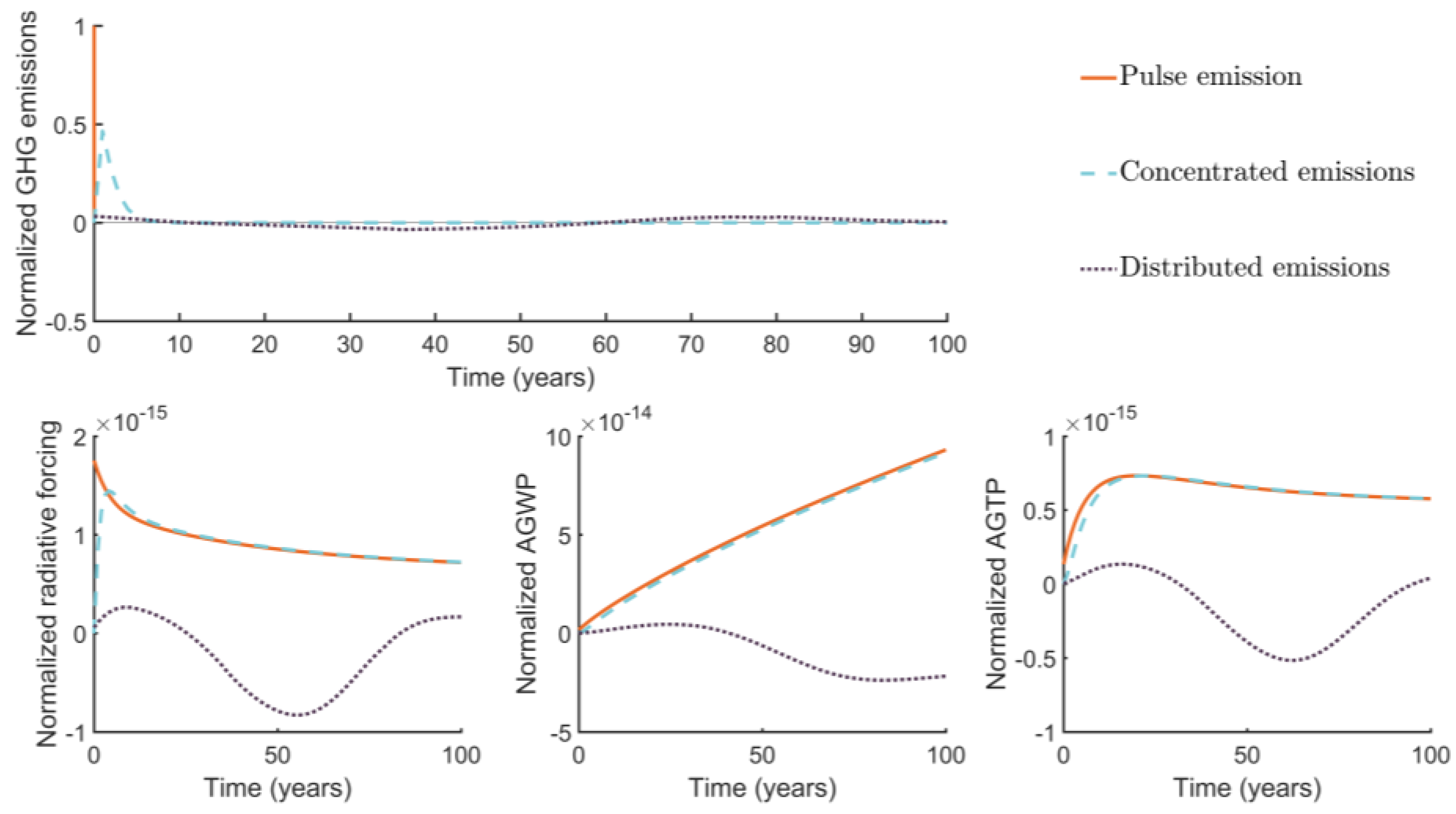
| GWP20 | GWP100 | GTP20 | GTP100 | |
|---|---|---|---|---|
| Pulse Emission | 1 | 1 | 1 | 1 |
| Concentrated Emissions | 0.91 | 0.98 | 0.99 | 1.00 |
| Distributed Emissions | 0.16 | −0.23 | 0.18 | 0.06 |
| DLCA | GWPbio | |
|---|---|---|
| Description | LCA framework | Emission metric |
| Initial Purpose | To solve inconsistency and time sensitivity issues in LCA | To assess the life impacts of regenerative biomass by integrating it with the global carbon cycle |
| LCI | Dynamic | Static—dynamic elements are included in the DCF |
| LCIA | Dynamic characterization factors, fixed endpoint | Dynamic characterization factors, fixed endpoint |
| Emission Metric | GWIinst, GWIcum; can be adapted to other metrics. | GWPbio, GTPbio; can be adapted to other metrics. |
| Sensitivity to TH | High | High |
| Advantages | Scales well for large amount of processes, if dynamic LCI data is available; Treats fossil and biogenic GHG emissions equally and simultaneously, using the same DCF. | Can be selectively applied to specific processes; Can be combined with other biogeophysical effects (e.g., albedo); Can be used within conventional LCA software; Might be useful for reporting biogenic carbon in EPD; Requires less data. |
| Potential Issues | Major LCI databases and LCA software do not currently support dynamic LCI; Using the DLCA framework to its full potential will only be possible after major DLCI data requirements are met. | Applying GWPbio only to selected processes can introduce inconsistencies; Using it in conventional LCA software might become tedious for large amount of processes (multiplication of unique DCF). |
© 2018 by the authors. Licensee MDPI, Basel, Switzerland. This article is an open access article distributed under the terms and conditions of the Creative Commons Attribution (CC BY) license (http://creativecommons.org/licenses/by/4.0/).
Share and Cite
Breton, C.; Blanchet, P.; Amor, B.; Beauregard, R.; Chang, W.-S. Assessing the Climate Change Impacts of Biogenic Carbon in Buildings: A Critical Review of Two Main Dynamic Approaches. Sustainability 2018, 10, 2020. https://0-doi-org.brum.beds.ac.uk/10.3390/su10062020
Breton C, Blanchet P, Amor B, Beauregard R, Chang W-S. Assessing the Climate Change Impacts of Biogenic Carbon in Buildings: A Critical Review of Two Main Dynamic Approaches. Sustainability. 2018; 10(6):2020. https://0-doi-org.brum.beds.ac.uk/10.3390/su10062020
Chicago/Turabian StyleBreton, Charles, Pierre Blanchet, Ben Amor, Robert Beauregard, and Wen-Shao Chang. 2018. "Assessing the Climate Change Impacts of Biogenic Carbon in Buildings: A Critical Review of Two Main Dynamic Approaches" Sustainability 10, no. 6: 2020. https://0-doi-org.brum.beds.ac.uk/10.3390/su10062020