Geographical Dynamics of Poverty in Nepal between 2005 and 2011: Where and How?


1
Institute of Mountain Hazards and Environment, Chinese Academy of Sciences, Chengdu 610041, China
2
Geography and Environment Academic Unit, University of Southampton, Southampton SO17 1BJ, UK
3
School of Geography and Environmental Science, Guizhou Normal University, Guiyang 500025, China
4
Central Department of Geography, Tribhuvan University, Kirtipur 44618, Nepal
*
Authors to whom correspondence should be addressed.
Sustainability 2018, 10(6), 2055; https://0-doi-org.brum.beds.ac.uk/10.3390/su10062055
Submission received: 17 May 2018
/
Revised: 13 June 2018
/
Accepted: 14 June 2018
/
Published: 17 June 2018
(This article belongs to the Section Economic and Business Aspects of Sustainability)
Abstract
:Poverty eradication is currently a central issue within the national economic development strategy in developing countries. Understanding the spatial changes and possible drivers of poverty from different geographical perspectives has the potential to provide a policy-relevant understanding of the trends in poverty. By district-level data, poverty incidence (PI), and a statistical analysis of the period from 2005 to 2011 in Nepal, we used the location quotient (LQ), as well as the Lorenz curve, to inspect the poverty concentration and the spatial-temporal variation of poverty in Nepal. As such, this study analyzed the change in identified typologies of poverty using an approach, which accounts for inter-regional and three identified terrain components. The PI methodological approach was applied in order to (i) compare the spatial change in poverty for Nepal during the study period from a geographical-administrative perspective and (ii) to develop Lorenze curves which show the change of poverty concentration over the study period. Within the Foster-Greer-Thorbecke (FGT) approach, PI was further used, in combination with the indices of poverty gap (PG) and squared poverty gap (SPG), in order to highlight the unidimensional poverty (UP), that is the incidence, depth, and severity of poverty between 2005 and 2011. Simultaneously, the spatial relationship between UP and economic development was assessed, leading to five specific economic modes or typologies of poverty. Our findings identified that proportional poverty appears to have grown in mountainous areas as well as more urbanized and developed regions, while the mid hill regions have steadily reduced proportions of poverty. We propose a hypothesis, for further examination, which suggests that the increase in proportional poverty in the mountain regions is as a result of the migration to the urban areas of Nepal of the relatively less poor, leaving behind a trapped poorer population. This migration to urban areas of the relatively less poor, rather counterintuitively, produced an increase in proportional poverty in the urban areas. This is due to the fact that while this population represents the wealthier mountain communities, they are still relatively poor in an urban setting.
1. Introduction
Poverty is both an objective (absolute) and subjective (relative) phenomenon that has been experienced throughout human social development [1], and poverty alleviation is a major challenge for all nations, especially developing countries [2,3,4]. Within scientific communities, the understanding of poverty has progressively deepened. Monetary poverty is the primary and initial stage of poverty [5,6]. With social development, the concepts of capability poverty and entitlement poverty were proposed by the Nobel Prize winner Amartya Sen in the 1980s [7,8], which broadened the understanding of poverty beyond its traditional economic context [1]. Such poverty is because of various factors, and the concept of multiple deprivation or multidimensional poverty has become extensively accepted with an increased focus on the union of material deprivation, social exclusion and limited empowerment, as well as psychological ill-being [9,10]. The Human Poverty Indicator (HPI) of UNDP is probably the first multidimensional poverty measure [11]. The HPI was obtained at national level based on the un-weighted sum of three sub-indicators: mortality rate; illiteracy and economic deprivation. In 2010, the HPI was substituted by the famous Multidimensional Poverty Index (MPI), which was fabricated for assessing the multidimensional poverty of 104 countries at household level [12]. For the latter, the index was aggregated from ten indices correspondence to three dimensions of education, health and living standard, on the basis of the specific deprivation thresholds identified normatively for each of the indices. Meanwhile, each dimension is empowered with equal weight in the calculation. To date, the MPI has been taken as a benchmark measure to inspect the aggregate poverty from developed countries [13,14] to developing countries [15,16,17] and the least developed countries [18,19], as well as from region scales [20,21] to local scales [22,23] around the world. With these extensive empirical analyses, the proposed policy implications not only illustrated how to evaluate the patterns and extent of multiple aspects of pro-poverty activities, but also identified subgroups with lagged dimensions of varied well-being attributes.
Although the defects of applying income to estimate an individual’s aggregate well-being are well recognized, there are continuing arguments over the appropriateness of amounting distinct dimensions of deprivation as a single measure for the multidimensional nature of poverty due to three main concerns [16,24,25,26]. Firstly, amounting indicators are condemned as overlapping, as well as covering the growth of each single trait once incorporated into the aggregated measure. Secondly, the method of aggregating varied well-being dimensions is disputed, especially as monetary indices are merged with non-monetary ones. In the last place, the concerns about the weighting formula for the dimensions involved are particularly increasing. Nevertheless, it was argued that thoroughly understanding the implicit trade-offs within distinct dimensions regarding specific indices may provide a key interlinked step to prompt the multidimensional deprivation research into a new development with respect to the aforementioned concerns [27,28].
Since the 1990s, nonetheless, there has been increasing attention given in academic circles to the geographic disparities in poverty and development outcomes [29]. As geographical studies related to poverty have become more common, spatial poverty has become the foundation of regional development and poverty alleviation strategies in some nations [30]. Spatial poverty has been used to explore differences in poverty from a geographical perspective in combination with environmental concerns [31]. Spatial diversity in poverty has been demonstrated in many countries in case studies of regional development and within urban-rural economic structures [32,33,34]. Decision makers in developing countries use spatial dimension of poverty when deciding how best to allocate resources at the local level [35,36]. Despite this, existing poverty studies have been less concerned with spatial poverty, focusing more on the connotation [37], methods [38,39] and scale issues [40,41,42]. Accordingly, investigating the poverty-environment relationship from a geographical perspective, i.e., across different locations and terrains, may enable poverty distribution and its underlying constraints and factors to be better understood [43,44,45,46].
Nepal is a country with diverse landforms, sensitive ecosystems, low natural resource setting, and a vulnerable human-environment relationship. As one of the most underdeveloped countries in the world, poverty is a long-standing problem for Nepal and poverty alleviation requires urgent attention. Since the 1970s, Nepal has instigated a range of poverty reduction and development programs [3], which have helped reduce poverty in the county, although there are still distinct problems, particularly in mountainous rural areas where the poverty gap remains large. Poverty research for Nepal has concentrated on the connection between poverty and income [47], the influence of migration and remittances on poverty [48,49], household livelihood options for the implication of rural pro-poverty [50], environmental reliance of household income and poverty reduction [51,52,53], public facilities or services for alleviating poverty in difficult terrains, such as rural road construction [54] and energy accessibility [55], as well as the nexus between poverty and political conflicts, including violence and wars [56,57,58].
There have been few investigations of the spatial differences of poverty and their drivers over time in Nepal. Nevertheless, Nepal is an appropriate location for investigating spatial poverty for two reasons. First, Nepal is considered to be one of the world’s most underdeveloped countries, ranking 145th in the Human Development Index in 2014. The nation has experienced a high occurrence of poverty and hunger for a long time. Second, the nation consists of diverse geographical features and ecological zones, such as the Tarai in the south (17% of its whole territory), the high hills in the central area (68% of its whole territory), and the high mountains in the north (15% of its whole territory). Each region shows distinct biophysical and socioeconomic features, which are accompanied by differences in the human-rural land relationship that are largely associated with the exploitation of natural resources.
Migration in Nepal is a well-studied phenomenon, with work identifying potential environmental drivers of migration [59], as well as clear economic, social and cultural incentives for migration from poorer, remote mountainous regions to the lower-altitude urbanizing centers [60], as well as more strategic seasonal migration [61]. Migration is contributing to the process of urbanization, with some of the highest rates of urban growth in the world, at 2% per annum with internal migration making up 45% of new income to cities. The dominant areas from which people migrate into the cities are the mountains [62]. This process is reflected in the higher poverty rates of urban settlements where migration is high and often in the suppressed labor markets [63]. Evidence to support this process can be found in the increase in poverty seen in sending areas; in Nepal, this includes mountainous regions, where populations who are unable to migrate can become trapped [64].
This study was designed to demonstrate spatial differences in poverty in Nepal, as well as its spatial dynamics in terms of geography from 2005 to 2011. Using the Foster-Greer-Thorbecke (FGT) poverty measures and the location quotient of poverty, as well as a simple computation method concerning the three aspects of the FGT measurement to determine unidimensional poverty, a more distinct dynamic of poverty evolution was obtained. The findings may improve our understanding of poverty distribution and its spatial features across a diverse range of geographical regions over time, as well as supporting the targeted development of poverty-related interventions for Nepal.
2. Materials and Methods
2.1. Study Area
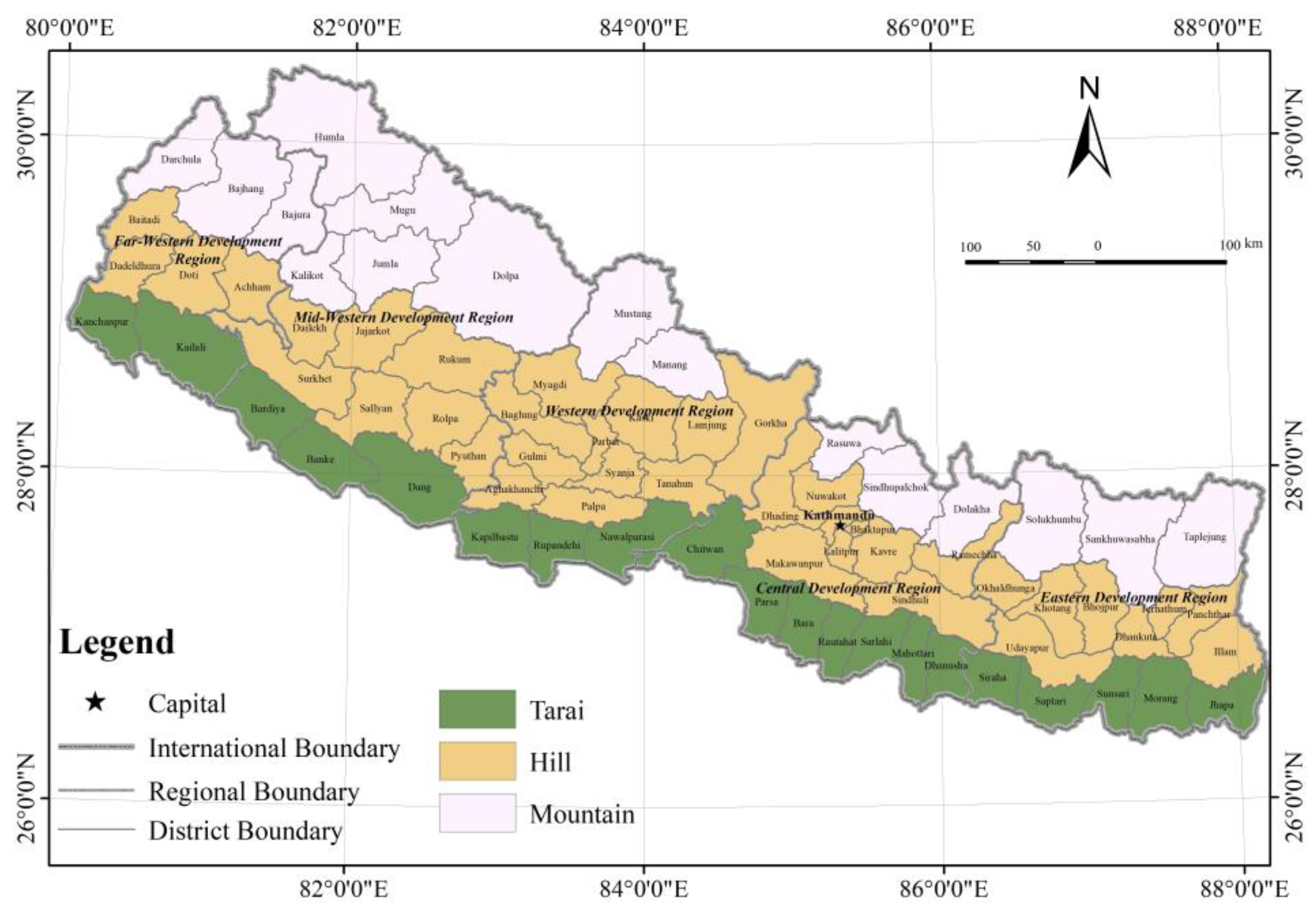
The study focused on spatial features and changes of unidimensional poverty (UP) from 2005 to 2011 in Nepal (Figure 1). Occupying an area of 147,181 km2 (26°22′ N–30°27′ N, 80°4′ E–88°12′ E) in South Asia, Nepal is a landlocked country, with an elevation range of 70 m to above 8000 m. In 2011, the annual population growth rate was 1.35%, with a total population of 26.5 million. According to its topographical conditions, there are three ecological zones in Nepal; that is, mountain, hill, and Tarai (i.e., flat plain), which contain 6.73, 43.00, and 50.27% of the total population, respectively. Nepal’s administrative units were changed after the state’s reconstruction of administrative divisions in 2015. However, our study was mainly based on the data at the district level, which changed relatively less and had no effect on poverty dynamics during the study period. Furthermore, during our study period, Nepal had five Development Regions for administrative purposes: the Eastern Development Region (the Eastern), the Central Development Region (the Central), the Western Development Region (the Western), the Mid-Western Development Region (the Mid-Western), and the Far-Western Development Region (the Far-Western). Based on the five Development Regions, the nation was further subdivided into 14 zones, as well as 75 districts during this period.
2.2. Data
For qualitative and quantitative analysis in our study, we used the population, area, the poverty incidence (PI), poverty gap (PG), and squared poverty gap (SPG) of Nepal between 2005 and 2011. Gross domestic product (GDP) per capita in 2011 (comparable price) at the district level was collected from the District & VDC Profile of Nepal (2014/15), 2011 Statistical Year Book and Nepal Human Development Report 2014. The three FGT indices of district-level in 2011 are the most recent and those in 2005 are the most early-stage data for Nepal. Some necessary geospatial information, i.e., boundary data of Nepal, was obtained from the International Centre for Integrated Mountain Development.
2.3. Methodology
2.3.1. Measuring Unidimensional Poverty and the Poverty Concentration
The FGT indices (Pa) introduced by Foster et al. [65,66] were applied to measure the UP of Nepal from 2005 to 2011. FGT, which is a class of decomposable poverty measures, was used to observe the incidence, depth, and severity of poverty, respectively, according to the value of a. For a = 0, 1, and 2, the FGT Pa refers to the head count ratio (i.e., poverty incidence, PI), the poverty gap (abbreviated to PG), and the squared poverty gap (SPG), respectively. SPG, which is similar to PG weighting for the poor based on how poor they are, gives the very poor a relatively greater weight than those who fall closer to the poverty line.
Moreover, for disclosing Nepal’s spatial concentration of poverty during the study period, we initially used the location quotient (LQ) [67], as well as the Lorenz curve, to investigate the poverty distribution among Development Regions, terrain zones, and different terrains in Development Regions.
2.3.2. Measuring PI, PG and SPG’s Spatial Differences.
We defined PI difference (PID), PG difference (PGD), and SPG difference (SPGD) as the change of PI, PG and SPG between 2005 and 2011, that is, PID = PI2011 − PI2005, PGD = PG2011 − PG2005, SPGD = SPG2011 − SPG2005. For district i (i = 1, 2, 3, …, 75), its PID, PGD and SPGD were respectively marked as PIDi, PGDi and SPGDi. The maximum and minimum PID, PGD and SPGD were recorded respectively as PIDmax (>0), PIDmin (<0), PGDmax (>0), PGDmin (<0), SPGDmax(>0) and SPGDmin (<0). In order to make the change of PI, PG and SPG more understandable and targeted, PIDs, PGDs and SPGDs were respectively reclassified into four grades as follows:
- (1)
- For PIDs, they were reclassified as ½ ×PIDmax > PIDi ≥ 0, PIDmax > PIDi ≥ ½ × PIDmax, ½ × PIDmin ≤ PIDi < 0, and PIDmin ≤ PIDi < ½ × PIDmin;
- (2)
- For PGDs, they were reclassified as ½ × PGDmax > PGDi ≥ 0, PGDmax > PGDi ≥ ½ × PGDmax, ½ × PGDmin ≤ PGDi < 0, and PGDmin ≤ PGDi < ½ × PGDmin;
- (3)
- For SPGDs, they were reclassified as ½ × SPGDmax > SPGDi ≥ 0, SPGDmax > SPGDi ≥ ½ × SPGDmax, ½ × SPGDmin ≤ SPGDi < 0, and SPGDmin ≤ PGDi < ½ × PGDmin.
2.3.3. Measuring Cluster Model of UP and Economic Development
The GDP per capita at the district level in Nepal in 2011 was selected to inspect the combination relationship between each of FGT indices (PI, PG and SPG) and economic development. Delaunay triangulation, which has been proven powerful for capturing spatial proximity and spatial clustering [68,69], was employed here to determine the cluster model of the combination relationship.
3. Results
3.1. Overall Trend of Poverty Change in Nepal from 2005 to 2011
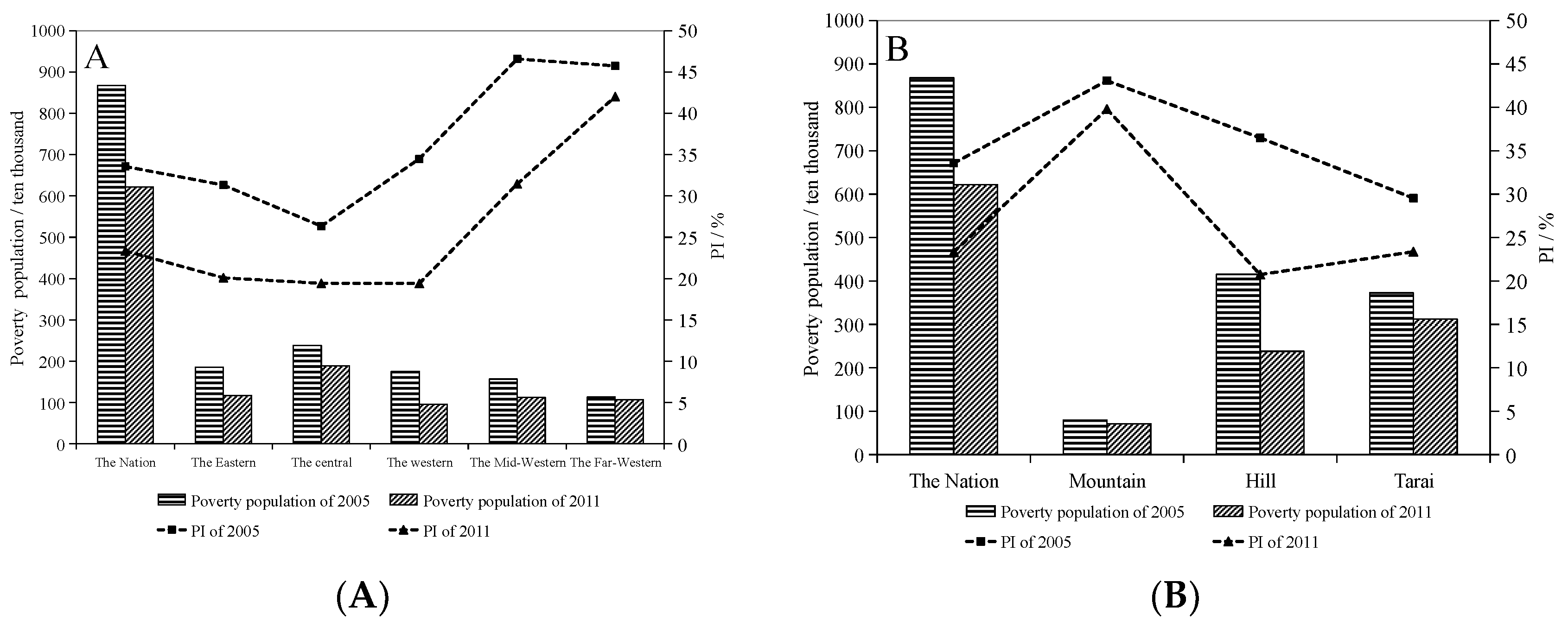
For the whole nation, as well as the five Development Regions and three terrain zones, the PI and poor people displayed gradually decreasing trends over the study period (Figure 2). Over the same period, the total number of poor people in Nepal decreased from 8.6778 million to 6.2144 million, with the PI decreasing from 33.57 to 23.34%.
As shown in Table 1, the PG and SPG of Nepal were 9.70 and 3.90% in 2005, respectively, while the corresponding values in 2010 were 5.43 and 1.81%. Moreover, the poverty LQ’s range and standard deviation in Nepal were 1.67 and 0.37 in 2005, respectively, while the corresponding values in 2011 were 2.57 and 0.57, respectively. Accordingly, the depth and severity of poverty across the whole of Nepal decreased from 2005 to 2010. However, the poverty distribution’s absolute and relative differences in Nepal increased during the same period.
In Development Regions, the largest decline for PI was seen in the Western, followed by the Mid-Western and Eastern (Figure 2A). A substantial decline was also observed in the Western, followed by the Mid-Western and Central regions. In the Far-Western, there was a weak decline in PI, while the number of poor people stabilized. A positive correlation was found between the changes in PI and poverty among the Development Regions over the study period. From Table 2, the PG and SPG of the Development Regions followed simultaneous declining trends. The magnitude of the decline was largest in the Western and Mid-Western. The poverty LQ’s range and standard deviation in Development Regions displayed a consistent increasing trend in the Western, Mid-Western, and Far-Western. Both of the indices referred to above presented decreasing trends in the Central, with the inverse pattern observed in the Eastern. Although the depth and severity of poverty in Development Regions has been alleviated, the absolute and relative differences of poverty among Regions revealed a complicated pattern. There were increasing trends in absolute and relative poverty in the Western, Mid-Western, and Far-Western, yet the Central showed a decreasing tendency. For the Eastern, there was an increasing tendency in absolute poverty, but a decreasing trend in relative poverty.
For terrain zones, a positive correlation was also found between the change of PI and poor people (Figure 2B). The order of the decline in PI and overall poverty was hill > Tarai > mountain. It can be seen from Table 3 that the PG and SPG of terrain zones all displayed downward trends over the study period. Compared to the mountain, the hill and Tarai zones had a larger magnitude of decline in PG and SPG. The poverty LQ range and standard deviation exhibited similar rising trends from 2005 to 2011. It is, therefore, obvious that the depth and severity of poverty in the terrain zones were alleviated; however, poverty’s absolute and relative differences increased in the three zones during the study period.
3.2. Poverty Concentration in Nepal from 2005 to 2011
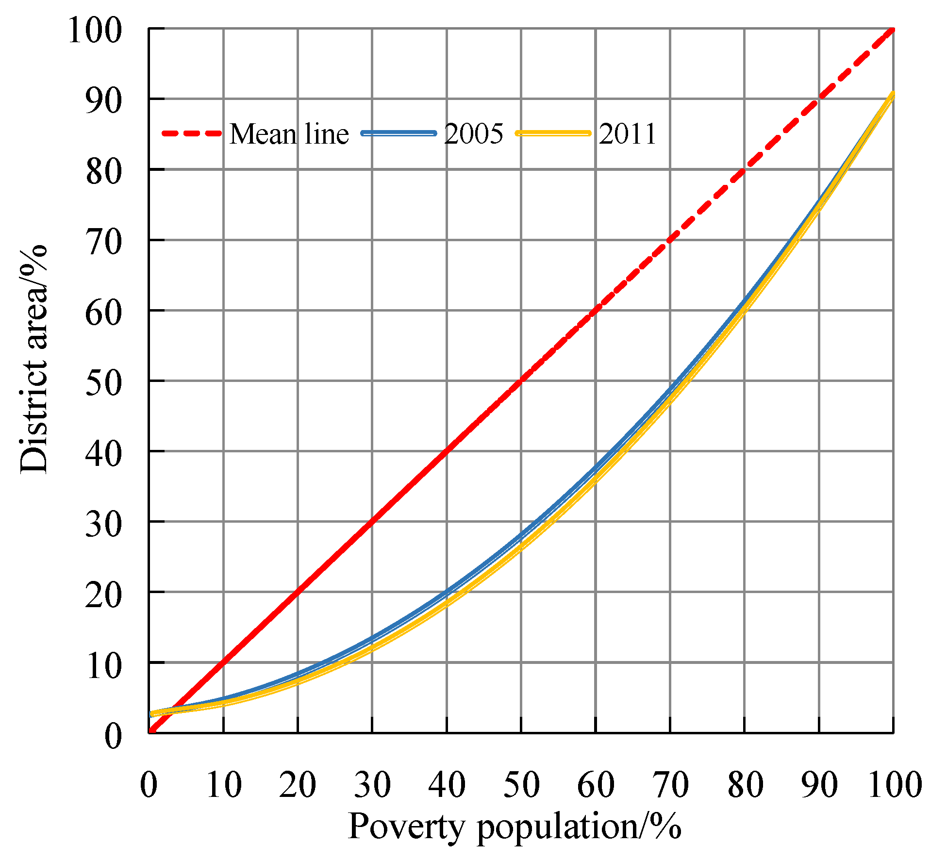
The Lorenz curve was applied to investigate the concentration of poverty in Nepal. As shown by Figure 3, around 72 and 73% of the population in poverty in 2005 and 2011, respectively, was located in 50% of the territory of the nation. This indicates that the concentration of poverty increased slightly during the study period.
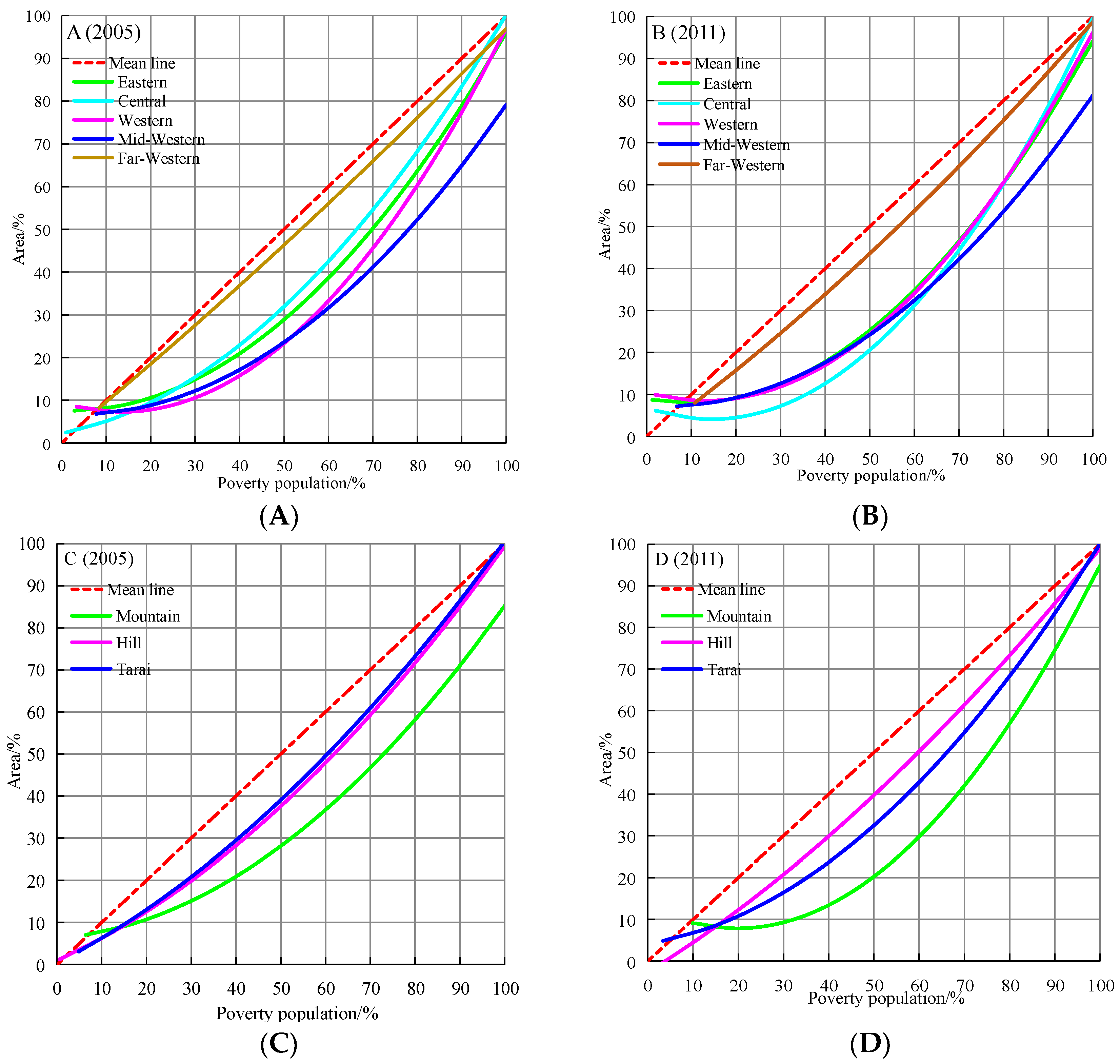
For Development Regions, around 71, 67, 76, 80, and 52% of poor people were located in 50% of the land area of the Regions from east to west, respectively, in 2005 (Figure 4A), while the corresponding values were 71, 75, 77, 80, and 55% in 2011 (Figure 4B). The Central experienced a marked spatial centralization, and the poverty centralization in the Western and Far-Western also increased by one and three percentage points, respectively. In addition to the increasing trend for poverty concentration, the extent of poverty concentration varied across the Regions in 2011. Poor people were more centralized in the Central, Western, and Mid-Western compared to 2005 as a whole, while that in the Far-Western presented a more even distribution.
In the different terrains, the concentration of the poor was very different among the mountain, hill, and Tarai zones. In 2005, 72% of the mountain poor lived in 50% of the territory, with the corresponding figures being 62% and 60% for the hill and Tarai zones (Figure 4C). In 2011, the corresponding figures were 76% in the mountain zone, 60% in the hill zone, and 66% in the Tarai zone (Figure 4D). Compared with 2005, by 2011 poor people had become more centralized, except for in the Hill zone.
3.3. PI Comparison for Three Geographical Divisions in Nepal from 2005 to 2011
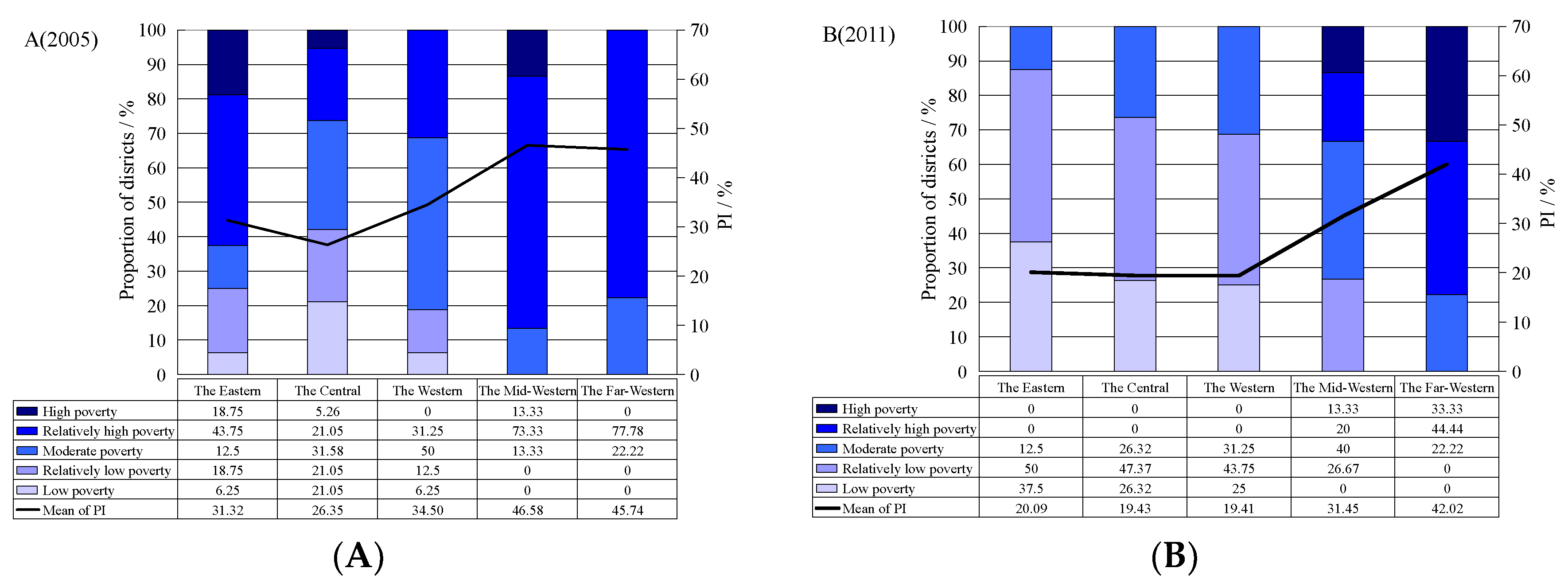
PI comparison was carried out across three geographical divisions: administrative areas (Development Regions), geographical areas (terrain zones) and geographical-administrative areas (different terrain zones in Development Regions). Moreover, according to the PI in 2005 and 2011, all the districts were classified into five grades, respectively: low (4%–16%), relatively low (16%–28%), moderate (28%–40%), relatively high (40%–52%) and high (more than 52%).
3.3.1. Administrative Divisions
For Development Regions, overall poverty levels of four Regions showed a reducing trend while only that of the Far-Western presented an increasing trend (Figure 5). As for the Eastern and Central in 2005, they contained districts where all five poverty ranks were prevalent, with the proportion of districts with high poverty being 18.75 and 5.26%, respectively, and those with relatively high poverty being 43.75 and 21.05%, respectively. In 2011, there were no districts in these two Regions with high or relatively high poverty, and the most relatively low poverty districts appeared among them. This indicates that the poverty of these two Regions decreased significantly over time. For the Western, the original four poverty ranks changed to three ranks. Districts with relatively high poverty accounted for 31.25% of all districts in 2005, whereas this figure became 0 in 2011. Additionally, the proportion of districts with low and relatively low poverty increased substantially. For the Mid-Western, its overall poverty also reduced by enlarging the proportion of moderate and relatively low poverty and diminishing that proportion of relatively high poverty. As for the Far-Western, its main rank was changed from relatively high (77.78%) in 2005 to relatively high (44.44%) and high (33.33%) in 2011.
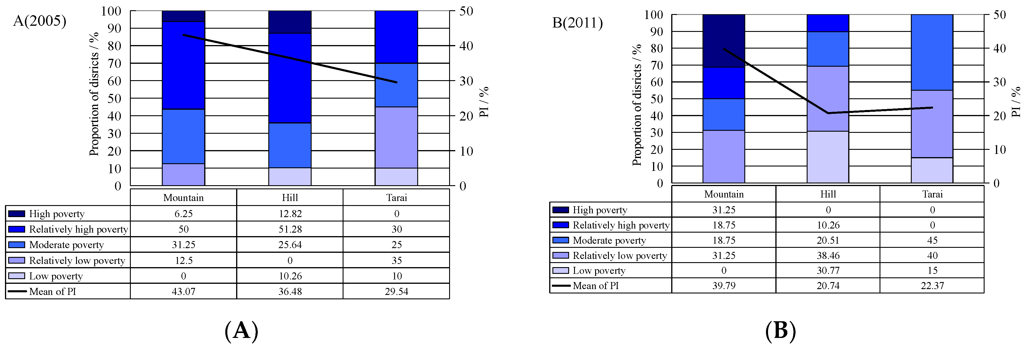
3.3.2. Geographical Divisions
From the perspective of terrain zones, overall poverty of hill and Tarai presented a reducing trend, as well as a homogenization tendency among districts (Figure 6). However, the poverty incidence of mountain zones showed an increasing trend, especially in the high poverty rank.
For the mountain zone, there were four poverty ranks with varying proportions prevalent during 2005–2011. The proportion of districts with relatively low poverty increased from 12.5% in 2005 to 31.25% in 2011, and that with relatively high poverty declined from 50% to 18.75%. However, the proportion of districts with high poverty increased from 6.25 to 31.25%. For the hill zones, there were also four poverty ranks prevalent, with obvious changes over time. The proportion of districts with high poverty declined from 12.82% in 2005 to 0% in 2011, while that with relatively high poverty decreased from 51.28% to 10.26%. The main poverty ranks in the hill region were relatively low and low poverty in 2011. As for the Tarai zone, there were also four poverty ranks in 2005, but only three ranks in 2011, with no high or relatively high poverty ranks. The proportion of districts with relatively high poverty declined from 30% to 0%, while that with low and relatively low poverty ranks increased.
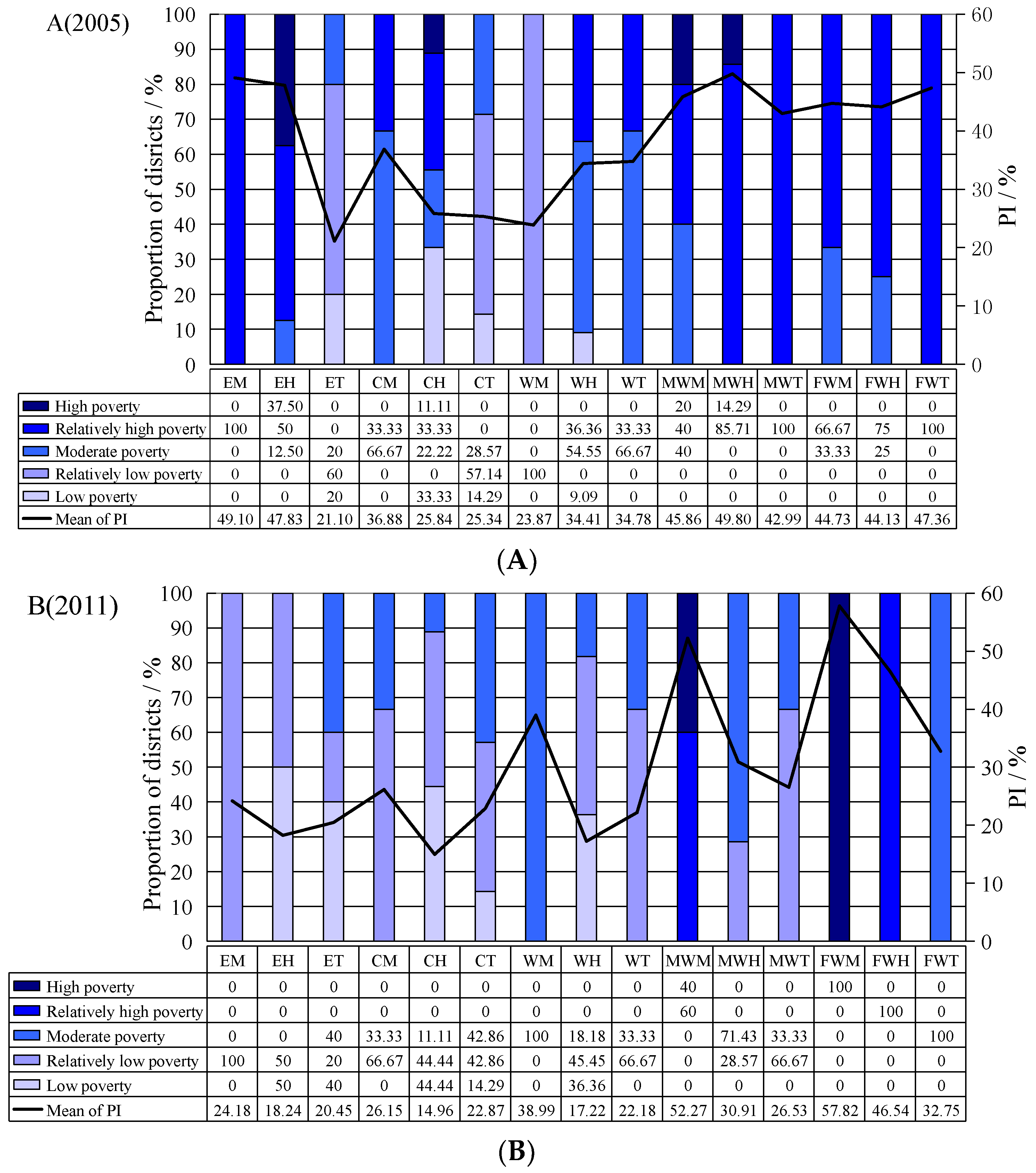
3.3.3. Geographical-Administrative Divisions
According to the distribution of Regions and terrain zones in Nepal, 15 sub-combination areas were named as Eastern Mountain (EM), Eastern Hill (EH), Eastern Tarai (ET), Central Mountain (CM), Central Hill (CH), Central Tarai (CT), Western Mountain (WM), Western Hill (WH), Western Tarai (WT), Mid-Western Mountain (MWM), Mid-Western Hill (MWH), Mid-Western Tarai (MWT), Far-Western Mountain (FWM), Far-Western Hill (FWH), and Far-Western Tarai (FWT). From Figure 7, the most significant change of PI among these sub-combination areas was that the high poverty and relatively high poverty ranks were concentered into the Mid-Western Mountain, the Far-Western Mountain, and the Far-Western Hill from 2005 to 2011. Additionally, the “relief” change of the curve (mean PI) showed a distinct trend that the relative differences among these sub-combination areas were broadened. The result was that the mountain zone of each Region became the area with maximum PI in the same Region.
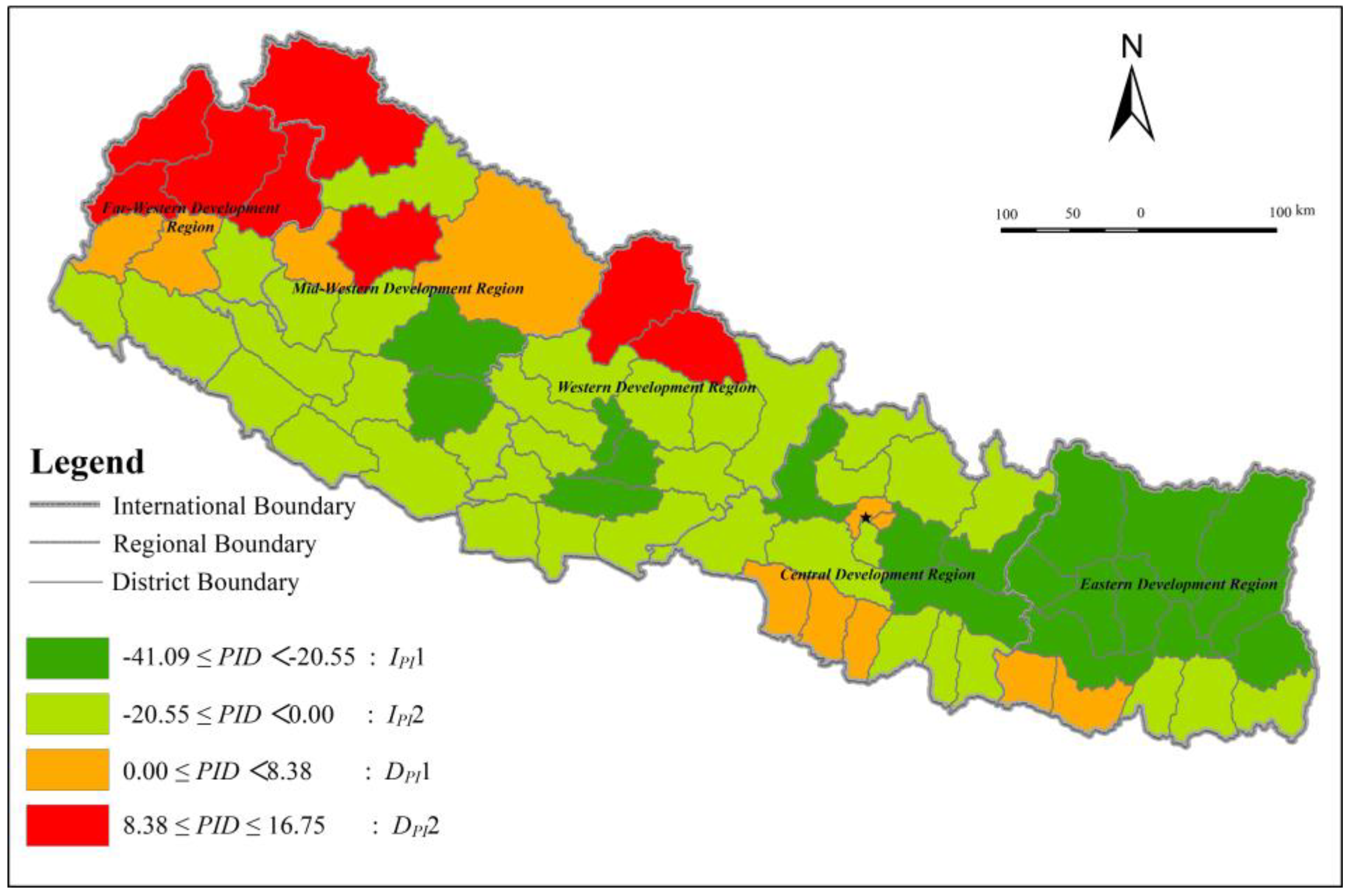
3.4. Spatial Change of UP Based on District Level in Nepal from 2005 to 2011
According to Section 2.3, the range of the PID for each district between 2005 and 2011 was classified into positive and negative. Positive PID indicated that PI increased from 2005 to 2011, and these districts are referred to as Increased PI. The districts with Increased PI were further classified into two sub-grades based on the degree of increase from low to high: Increased PI 1 (IPI 1) and Increased PI 2 (IPI 2). Negative PID indicated that PI reduced during the study period, and these districts are referred to as Reduced PI. The districts with Reduced PI were also classified into two sub-grades based on the degree of reduction from low to high: Decreased PI 1 (DPI 1), Decreased PI 2 (DPI 2). Similarly, for PGD and SPGD, they were also further classified into four sub-grades, respectively: Increased PG 1 (IPG 1), Increased PG 2 (IPG 2), Decreased PG 1 (DPG 1), and Decreased PG 2 (DPG 2); and Increased SPG 1 (ISPG 1), Increased SPG 2 (ISPG 2), Decreased SPG 1 (DSPG 1), and Decreased SPG 2 (DSPG 2).
3.4.1. The Spatial Change of PI at the District Level
With regard to the PI change in Development Regions during the study period, except the Far-Western, the other four Regions in Nepal all showed a distinct overall decreasing trend (Table 4 and Figure 8). About 25% of the districts presented Increased PI, most of which were located in the Far-Western, Central and Mid-Western. Only 2 of 16 districts showed increasing PI both in the Eastern and Western. Additionally, the Eastern indicated a sounder PI decrease, as its DPI2 was much bigger than that of the Western. Meanwhile, the districts with decreased PI occupied 75% of the whole nation, most of which was found in the Eastern, the Central and the Western. Although the number of districts with Decreased PI in the Western was the same as that of the Central, the Western held fewer districts with Increased PI. Therefore, the most obvious PI decrease occurred in the Eastern, followed by the Western and the Central. The least PI decrease was the Far-Western, followed by the Mid-Western.
For terrain zones, there were 34 of 39 districts showing Decreased PI in the hill zone, while that number was seven of 16 and 15 of 20, respectively, in the mountain and Tarai zones. This means that PI decreased at a proportionally greater rate in the hill zone than the other two terrain zones from 2005 to 2011. Furthermore, the mountain zone shows the worst performance for PI decrease.
3.4.2. The Spatial Change of PG at the District Level
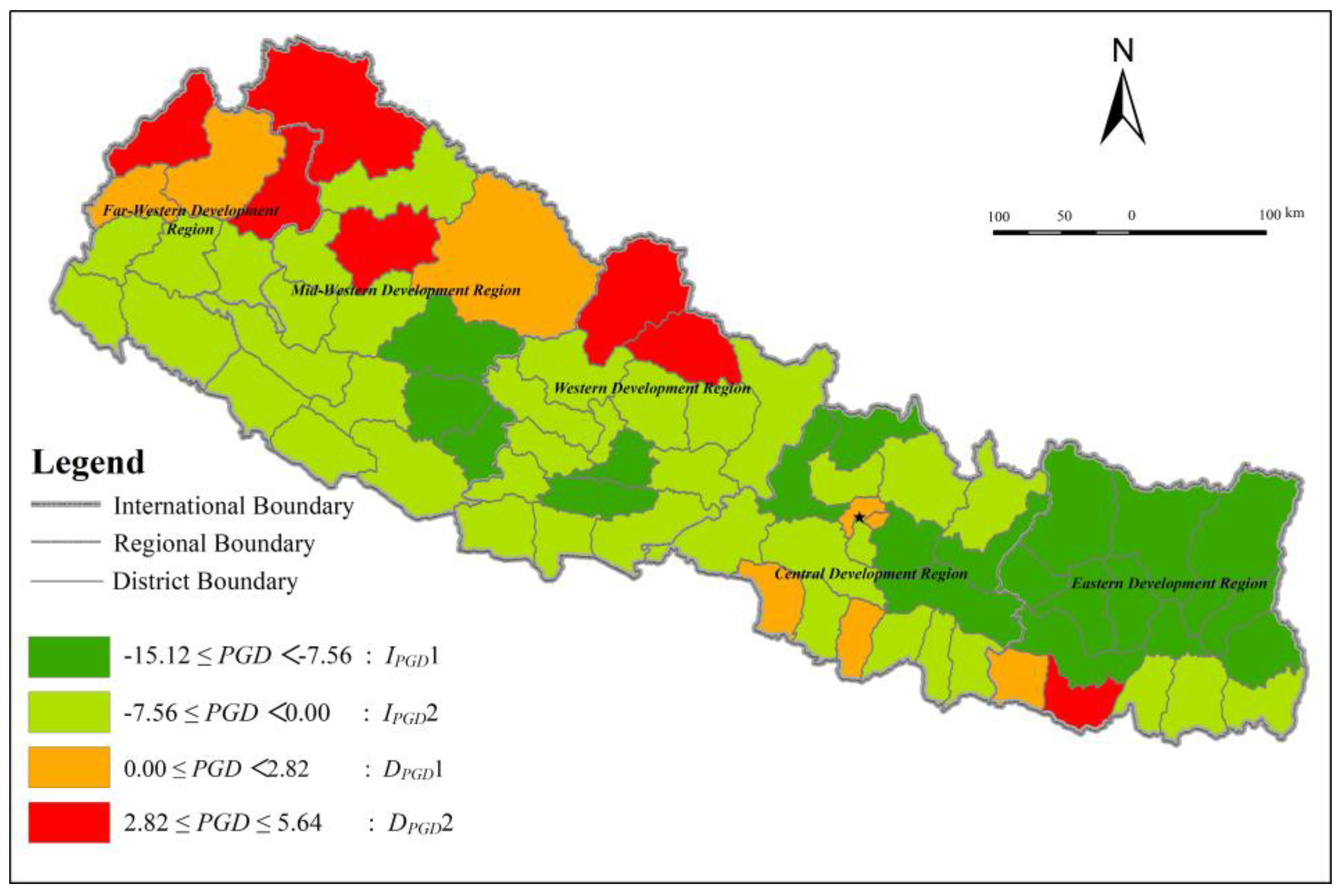
When inspecting the PG change in Development Regions, it exhibited an overall decreasing trend for the same four Regions, as their PG decreased from 2005 to 2011 in Nepal (Table 5 and Figure 9). 20% of the districts presented Increased PG, most of which were located in the Far-Western and Central. There were only 2 of 16 districts that showed an increasing PG in either the Eastern or Western. In addition, the Eastern exhibited a better PI decrease, as its DPI2 was much bigger than that of the Western. At the same time, the districts with decreased PI accounted for 80% of the nation, most of which were in the Central, Eastern, Western and the Mid-Western. Therefore, the most obvious PG decrease occurred in the Eastern, followed by the Western and the Central. The worst performance for PG decrease was the Far-Western, followed by the Mid-Western.
Physiographically, there were 36 of 39 districts with Decreased PG in the hill zone, while that number was 8 of 16 and 16 of 20 in the mountain and Tarai zones, respectively. Accordingly, from 2005 to 2011 in Nepal, the greatest decline of PI was evident in hill the zone, followed by the Tarai zone. The mountain zone performed worst for decreasing PG during the study period.
3.4.3. The Spatial Change of SPG at the District Level
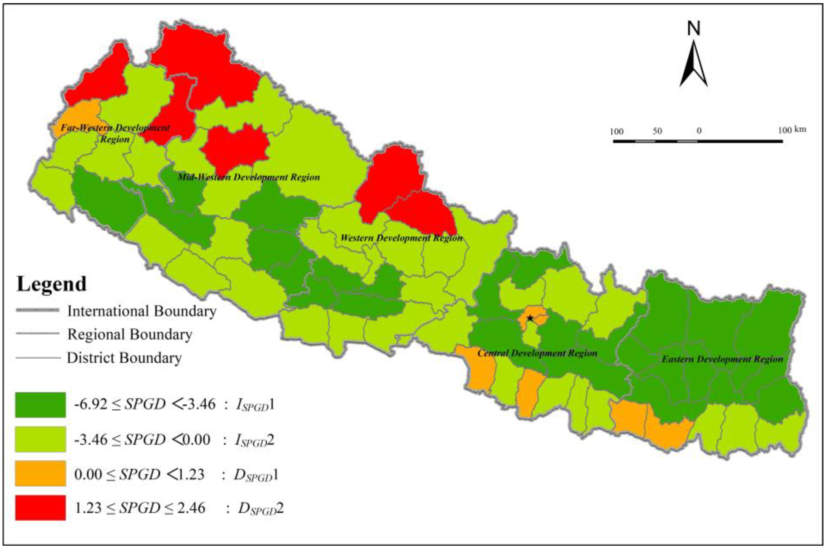
As for the SPG change in the Development Regions from 2005 to 2011 in Nepal, the overall decreasing trend was indicated more obviously (Table 6 and Figure 10). Around 17% of the districts showed Increased SPG, most of which were in the Central. For the Eastern, Western and Mid-Western, the number of districts with Increased SPG was all the same, i.e., two. While in the Far-Western, that number was three. Meanwhile, the districts with Decreased SPG occupied 83% of the country, most of which was in the Central, Eastern, Western and the Mid-Western. Hence, the Eastern presented the best performance for SPG decrease, followed by the Central and the Western. Additionally, the worst performance for SPG decrease was in the Far-Western, followed by the Mid-Western.
From the perspective of terrain, there were 36 of 39 districts with Decreased SPG in the hill zone, with that number being 10 of 16 and 16 of 20, respectively, in the mountain and Tarai zones. Hence, during the study period in Nepal, the greatest SPG decline happened in the hill zones, followed by the Tarai zone. Additionally, the mountain zone still performed worst for decreasing SPG from 2005 to 2011.
3.5. Combination of UP and Economic Development at the District Level in Nepal in 2011
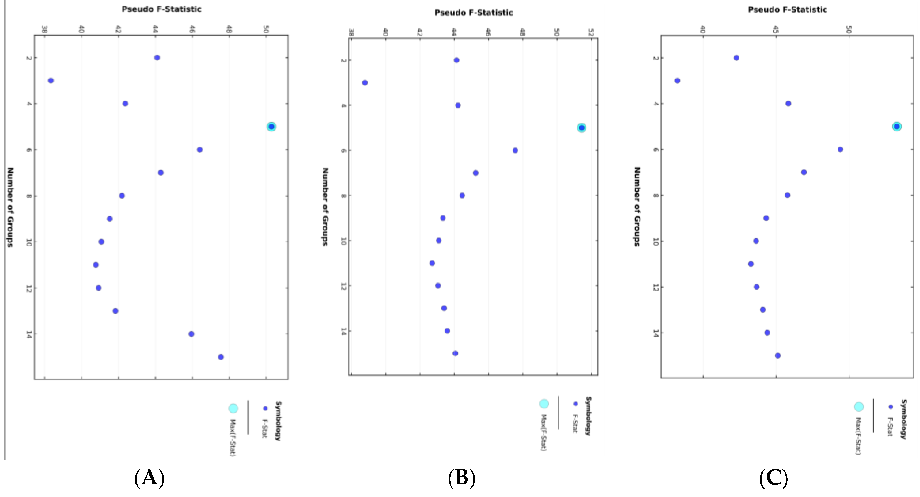
GDP per capita of each district in Nepal was used to describe the nation’s development level of economic activities in view of the district scale. Delaunay Triangulation Clustering, which is powerful for capturing spatial proximity and clustering [70], was employed here to investigate the combination relationship of UP and economic activities for Nepal in 2011. From the pseudo-statistical results (Figure 11), it was demonstrated that the proper number of the combination groups to indicate the combination models between economic activity and each of FGT indices (PI, PG and SPG) was supposed to be “5”. In addition, Table 7 also clarifies the parameters for the combination models.
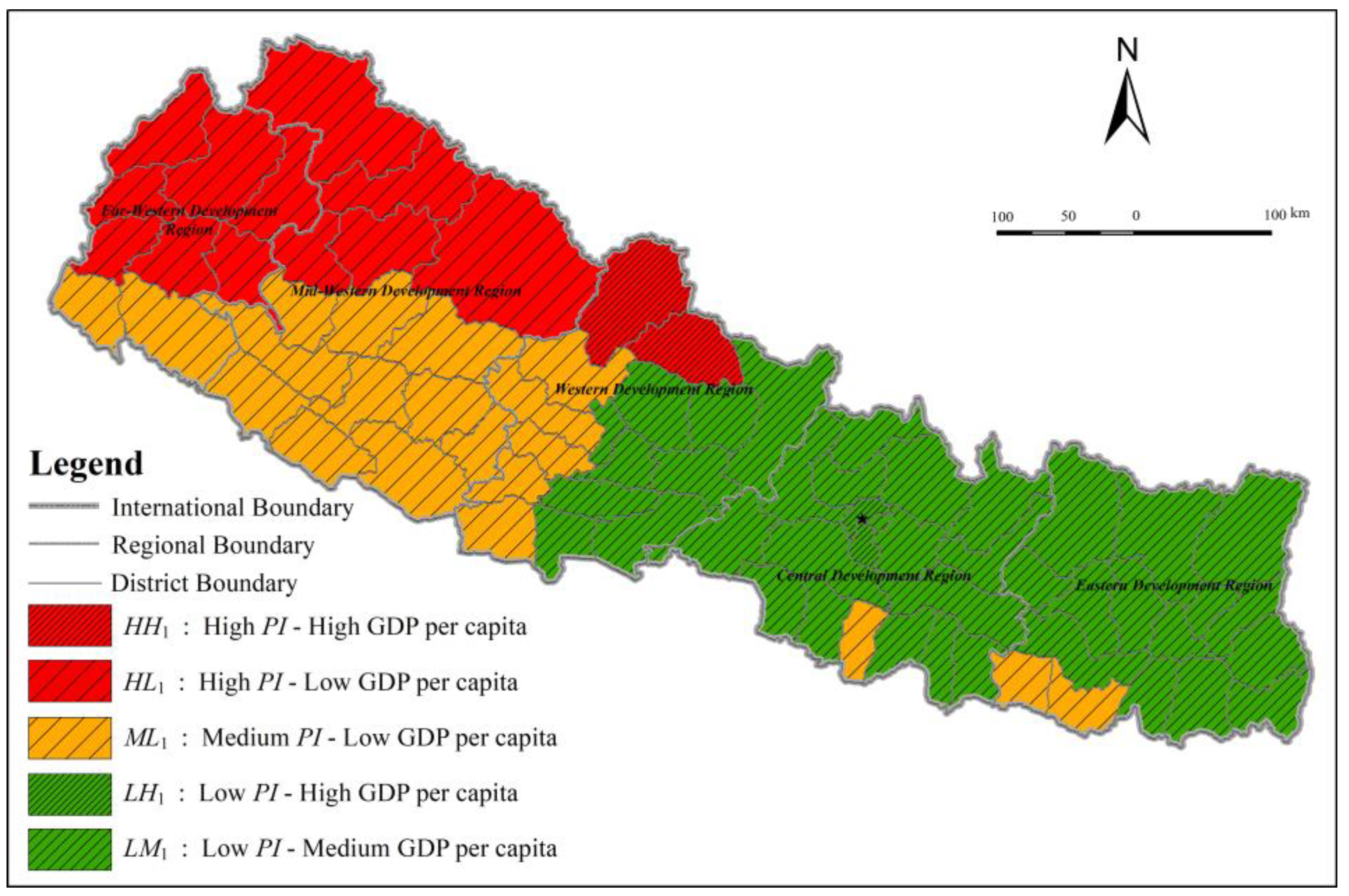
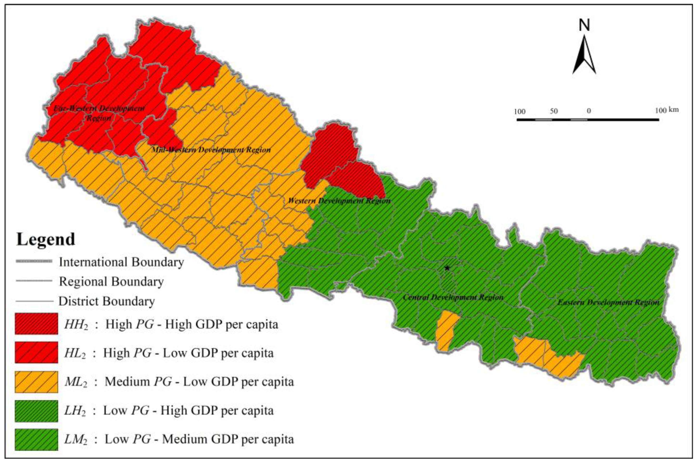
Consequently, the combination models for PI-GDP per capita combination, PG-GDP per capita combination and SPG-GDP per capita combination are listed as Figure 12, Figure 13 and Figure 14, respectively. For the PI-GDP per capita combination (Figure 12), the five models are as follows: High PI-High GDP per capita (HH1), High PI-Low GDP per capita (HL1), Medium PI-Low GDP per capita (ML1), Low PI-High GDP per capita (LH1), and Low PI-Medium GDP per capita (LM1). For the PG-GDP per capita combination (Figure 13), the five models are as follows: High PG–High GDP per capita (HH2), High PG-Low GDP per capita (HL2), Medium PG-Low GDP per capita (ML2), Low PG-High GDP per capita (LH2), Low PG-Medium GDP per capita (LM2). For the SPG-GDP per capita combination (Figure 14), the five models are as follows: High SPG-High GDP per capita (HH3), High SPG-Low GDP per capita (HL3), Medium SPG-Low GDP per capita (ML3), Low SPG-High GDP per capita (LH3), Low SPG-Medium GDP per capita (LM3).
As shown by Figure 12, Figure 13 and Figure 14, for the combination modes of PI-GDP per capita, PG-GDP per capita and SPG-GDP per capita, three patterns, HL, ML and LM, occupied around 95% of all the districts. Additionally, the other two patterns of combination models, HH and LH, were found in the same districts. Furthermore, the former three patterns matched with the anticipation that economic development would be boosted and have a positive correlation with poverty alleviation, and vice versa. The latter two patterns only covered a very limited part of the nation. The HH pattern means that the high FGT indices (PI, PG and SPG) was closely related with the high level of economic development. Therefore, the HH pattern is inconsistent with this expectation. The two districts, Mustang and Manang, with the HH pattern, the UP of which was covered by the performance of a higher GDP per capita. The LH pattern was only located in Kathmandu and Bhaktapur, in the Kathmandu Valley, the most developed place in Nepal.
Moreover, the combination modes for PI-GDP per capita were little different from those of the PG-GDP per capita and the SPG-GDP per capita, which presented the same distribution across the whole nation. Obviously, the Western played the role of a border dividing the low and medium GDP per capita of districts. In the west of the Western, the main combination modes for districts were HL and ML. Meanwhile, in the east of the Western, the districts were dominated by the combination model of LH.
4. Discussion
(1) While PI measures the proportion of the poor, it cannot demonstrate the extent of the poor. Likewise, PG cannot show the difference of poor inequality. Considering poverty inequality, the SPG was constructed by averaging the squares of PG relative to the poverty line, identifying those who fall far away from the poverty line. Comparing the change of PI, PG and SPG in Nepal from 2005 to 2011, there was not only a “degree” change, but also a “direction” change for specific districts. Here, degree changes of PI, PG and SPG mean that the classifications for PID, PGD and SPGD of specific district vary only with Reduced or Increased. Whereas, the direction change of those means that the classifications among PID, PGD and SPGD for specific district vary across Reduced and Increased. Most of the districts kept the same classifications or showed the same degree change for PID, PGD and SPGD in the study period. This indicates that the proportion of poor people, poverty depth and the situation of the poorest at the district scale changed synchronously throughout most of Nepal from 2005 to 2011. Specifically, there were 13 districts with increased PI, increased PG and increased SPG during the period (Table 8). At the same time, there were six districts with a direction change, most of which were located in the Mid- and Far-Western, as well as the mountain and hill zones. Although only six districts with a direction change were identified (Table 9), it was helpful for policy making for targeted poverty elimination. As shown in Table 9, the proportion of the poor (PI) in the six districts increased; nevertheless, their PG and SPG decreased, which indicates that the average depth of poverty (poverty gap) narrowed, while the situation of the poorest also improved.
The change differentiation of PI, PG and SPG together provided a useful reference for Nepal’s poverty elimination. According to Table 8, the 13 districts showed a deteriorating trend of poverty change, as the PI, PG and SPG all increased. These districts are supposed to be the key area for poverty alleviation. From Table 9, the proportion of the poor in the six districts was identified as increasing simultaneously with the mitigation of poverty depth of the general poor as well as the poorest. For the other 56 districts, PI, PG and SPG all showed an improving trend, as all three indices decreased. Therefore, poverty reduction actions in the future for the nation should consider the following order of priority: the 13 districts, the six districts, and the other 56 districts.
(2) In 1990, poverty elimination started to attract priority political focus in Nepal, although the economic and poverty have attracted attention since the nation’s planned development. Since then, the Ninth Plan (1997–2002), with the main aim of poverty alleviation, was developed as a part of a 20-year long-term action plan. Then poverty reduction was deemed to be the overriding target in the Tenth Plan (2002–2007), which was formulated on the basis of the Poverty Reduction Strategy Paper (PRSP) [71]. Guided by Poverty Alleviation Fund (PAF) Ordinance 2003, the PAF has been established in Nepal. Nowadays, the poverty alleviation activities work under the PAF Act 2006 [72]. The ultimate objective of PAF was to diminish the population living in extreme poverty through the approaches of setting a demand-driven program, directly funding communities as well as sharing community costs as per targeted pro-poor guidelines, consideration of social inclusion, and transparency. Lowering the poverty incidence to 10 percent by 2017 was proposed as one of PAF’s main goals. Between 2004, when PAF started, and 2012, all 75 districts in Nepal were covered by the PAF program, with a total grant of around USD 150 million invested into Community Organizations (COs) of local districts. Apart from the PAF program, the Youth and Small Entrepreneur Self-Employment Fund, the Foreign Employment Program, and the Western Upland Alleviation Project were implemented throughout the entire county for combatting poverty.
Completing more than 55 years of planned development, as well as implementing varied pro-poor activities and programs, obvious positive impacts were witnessed for the poor, such as consumption ability rising, food insecurity reducing, income increasing, social inequity decreasing, and school attendance and women’s empowerment improving. However, the nation is not able to sustain the growing employment demand for economically active labor, especially for those who live in marginalized communities in remote mountains, such as the Mid-Western and Far-Western Regions [71]. Even the Western Upland Alleviation Project, which was one of few poverty interventions only targeting the mountainous environment, was still not satisfactory, due to the relatively low quality of training for local participating members (communities) in business enterprises, the inadequacy of the delivered service, knowledge handling, and so on [73].
(3) Confined by the data, we did not analyze the change of economic development or investigate the combination mode of economic change and UP change in Nepal from 2005 to 2011. The latter might be more sensitive to the correlation between poverty eradication and economic development in Nepal. However, the GDP per capita is one of the most commonly used indicators for observing a nation’s economic development and is relatively stable over quite a long term. Therefore, our analysis regarding the combination of UP and economic development of Nepal in 2011 is still relatively reliable.
Furthermore, we used total value-added proportion, as well as the employed population distribution of three major industrial sectors, to express the productive structure and the employment level for Development Regions of Nepal during the study period. In Table 10 and Table 11, the productive structure and the employment level together empirically indicate the close relatedness between economic development and poverty change, specifically for the Western, the Mid-Western and the Far-Western Regions, as well the mountains. From 1995 to 2010, around 50% of the poverty eradication observed in Nepal relied on labor income growth, especially for nonagricultural activities [71]. Specifically, the second half of the 2000s witnessed a succession of unprecedented increase in remittances on the share of GDP, from 15% in 2005 to 22% in 2010 [74]. There was no doubt that non-agricultural income, including migrants working abroad, underscored a significant role for poverty reduction. As such, the continued heavy reliance on primary sectors (including agriculture, fisheries and forestry), with the lackluster improvement of secondary and tertiary industries, as well as the low proportion of non-agricultural labor, coincided with the poor performance of poverty alleviation during our study period in the mentioned regions.
(4) The observed poverty trends across Nepal showed a clear alignment with the terrains, which was then modified in relation to the urban centers. In the simplest sense, it is possible to interpret the observed result as being the result of migration from the mountainous areas to the lowlands and hill tract urban centers, along with the continued development of the central hill regions. This was reflected in the increase in proportional poverty in the lowland regions, particularly in the west, and in the Kathmandu Valley as a result of the arrival of relatively poor migrants, predominantly from the western mountain regions. The increase in poverty proportion in the Western mountainous region, then, being a reflection of the residual trapped population who are not financially able to migrate, is a phenomenon that has been widely recognized in the migratory literature. This phenomenon is particularly prevalently expressed in the east and in the Kathmandu Valley. The increase in the proportion of poverty in the lowland regions and urban centers may also be assisted by the nature of proportional statistics, where it becomes harder and harder to elicit the same proportion of growth over a larger overall economy. The hill areas, which primarily occupy the mid latitudes of the country, except for in the east, where the hills penetrate further up the country, showed the greatest proportion of growth. This was interpreted as being the consequence of the tendency to have early gains in development as areas open up for development, as well as the simple fact that it is easier to proportionally develop an economy from a low starting point. Finally, the mountain areas, like the lowland areas of the south, lost their relatively less poor populations to migration while still being highly inaccessible for development, and as such they remain areas of declining population density but increasing deprivation.
(5) The outcome of our poverty analysis was crudely and primarily defined by monetary/income poverty (unidimensional poverty), employing the official statistical information of three FGT indices at a district level. This definition, as well as the related calculations, have been criticized due to its inadequate depiction of a wider and multiple deprivation profile for human well-being [12]. Nonetheless, for the most severely impoverished countries in Sub-Saharan Africa and South Asia, the economic background underpinning income poverty keeps playing a fundamental role in constricting general living and the development of conditions of health and education, as well as living standards, especially when the nation cannot deliver adequate basic public services, such as piped water, electricity, cooking fuel or sanitation [24]. As for our study, the Nepalese poor’s economic well-being is much more related with the aforementioned basic facilities, against a background of sluggish economic growth with very few exports, as well as high population growth with high dependency of the rural population on the primary industrial sector [74]. In addition, Nepal offers research potential for studying spatial poverty induced by terrain and geographical environment at a country level. Due to data accessibility, our study period was limited to the period from 2005 to 2011 in Nepal. However, compared with the existing studies on Nepal poverty [4,19,22,23,47,48,49,50,51,52,53,54,55,56,57,58,59], this study provided a contextual background on the overall trend of poverty change, the poverty concentration, the spatial change of UP (PI, PG and SPG), and the combination mode of UP-economic development along different dimensions and at district scales. This provided the opportunity to elucidate and consider potential drivers of development at a national scale.
Consequently, we argue that our conceptualization of poverty measures might be questioned in terms of its appropriateness; however, the novelty of the findings originating from multi-geographical analysis should not be diminished. With new and credible socio-economic and environmental data access in the future, we understand that it would be more impressive to utilize a similar multi-geographical perspective to observe multidimensional poverty and diversified deprivations in Nepal. Additionally, Nepal’s districts are usually heterogeneous in terms of social and environmental conditions. There may be geographic or administrative units smaller than districts that could better reflect the refined spatial texture of poverty dynamics, as well as being beneficial to illustrating the potential factors driving poverty change. The period from 2005 to 2011 is critical to the nation, as it coincided with the half decade of unsettled post-conflict recovery after a violent and enervating Maoist conflict, as well as being the period in which Nepal’s overall economy shuddered forward and started to have an inferior economic growth of around 3% to 4% [74]. Additionally, this paper aims to utilize the available secondary data to make an assessment of poverty in Nepal from 2005 to 2011, which is a critical period for the country, as illustrated. Therefore, the study was designed to address the quantitative issues surrounding the metrics of poverty, and as such does not address many of the qualitative issues. Such a combined approach would certainly be territory for further research in this area, but would require a sampled field strategy beyond the financial scope of the work outlined. All the same, more research will be attempted and conducted through the combination of quantitative as well as qualitative approaches in the future. This notwithstanding, from the multi-geographical perspective, this research is the first to have investigated the contextualized background of Nepal’s poverty dynamics from 2005 to 2011 through extensive analysis and based on the available data to date.
5. Conclusions
Based on FGT indices and the GDP per capita of Nepal at a district scale, this study investigated the UP change and poverty concentration in Nepal from 2005 to 2011 based on administrative and geographical divisions, as well as the combination relationship between each of the FGT indices (PI, PG and SPG) and the economic development of Nepal in 2011. We came to the following conclusions:
- The overall poverty in Nepal showed a downward trend from 2005 to 2011. As well as the Development Regions and terrain zones, the PI, PG, SPG and poor people displayed gradually decreasing trends over the study period. In terms of the extent of decrease of PI and poor people, the Far-Western and mountain zone displayed a downward trend, but to a lesser extent. Moreover, the poverty LQ’s range and standard deviation in 2005 in Nepal were lower than that in 2011. Except for the Central, the ranges of the poverty LQ in the other four Regions in 2011 were bigger than those in 2005. Except for the Eastern, the standard deviations of the poverty LQ in in the other four Regions in 2011 were bigger than those in 2005. For the three terrain zones, the ranges and standard deviations of the poverty LQ in 2011 were bigger than those in 2005.
- For the poverty concentration in Nepal, it was found that the concentration of poverty for the whole nation in 2011 was greater than that in 2005 based on the Lorenz curves of poverty distribution. As for the Regions, poor people had become more centralized in 2011 than they were in 2005 in the Central, the Western, and the Mid-Western. However, in comparison to other Regions, poor people in the Far-Western showed a more even distribution over the study period. Similarly, in the different terrains, more poor people were centralized in the mountain and hill zones. Overall, the agglomeration of overall poverty increased over the period studied.
- From the PI comparison carried out for the administrative, geographical and geographical-administrative dimensions, varied changes were observed during the study period. For Regions, the overall poverty of four Regions showed a reducing trend, while that of the Far-Western presented an increasing trend, and the poverty of the Eastern and Central decreased significantly over time. As for the terrains, overall poverty in the mountain zone increased, but it decreased in the hill and Tarai zones. In terms of the sub-combination areas under the geographical-administrative dimension, the most significant change of PI was that the high poverty and relatively high poverty ranks were concentered into the mountains of the Mid-Western and Far-Western, and the hill area in the Far-Western.
- According to the district-based spatial change of three FGT indices in Nepal, different changes of PI, PG and SPG were inspected. Firstly, the most obvious PI decrease happened in the Eastern, followed by the Western and the Central, and the worst PI decrease occurred in the Far-Western, followed by the Mid-Western. Secondly, the most obvious PG decrease occurred in the Eastern, followed by the Western and the Central, and the worst performance of PG decrease was found in the Far-Western followed by the Mid-Western. Thirdly, the best performance of SPG decrease was in the Eastern, followed by the Central and Western, and the worst SPG decrease was in the Far-Western, followed by the Mid-Western. Additionally, for the decrease of all three FGT indices, the mountain zone performed worst, followed by the hill and Tarai zones.
- By Delaunay Triangulation Clustering, five-pattern clustering was thought to be able to best describe the spatial relationship of UP and economic development. Three patterns, HL, ML and LM, in accordance with common logic, accounted for 95% of all the districts. The other two patterns, HH and LH, were observed in the same locations, taking a very limited part. The HH pattern did not stay in step with the common understanding, but the LH pattern did, just sitting in the main part of the Kathmandu Valley. Furthermore, the combination modes of PI-GDP per capita varied with those of PG- and SPG-GDP per capita. The latter exhibited the same location in the country. The Western Development Region was the border of low and medium GDP per capita at the district scale. The main combination modes for districts were HL and ML in the west of the Western, and the districts in the east of the Western were dominated by LH.
Author Contributions
J.Z. and C.H. conceived and designed the research; J.Z. and C.L. collected and processed the data; J.Z., C.L. and C.H., H.L.K. analyzed the data. All authors have read and approved the final manuscript.
Funding
This research was funded by the NSFC-ICIMOD Cooperation Project (NO. 41661144038-02), the 135 Strategic Program of the Institute of Mountain Hazards and Environment, Chinese Academy of Sciences (NO. SDS-135-1708), the Youth Innovation Promotion Association of Chinese Academy of Sciences (NO. 2018407), and the State Scholarship Fund of China (NO. 201704910247).
Acknowledgments
The authors would like to thank the anonymous reviewers for their insightful comments and suggestions on the paper.
Conflicts of Interest
The authors declare no conflict of interest.
References
- Liu, Y.; Xu, Y. A geographic identification of multidimensional poverty in rural China under the framework of sustainable livelihoods analysis. Appl. Geogr. 2016, 73, 62–76. [Google Scholar] [CrossRef] [Green Version]
- Grindle, M.S. Good enough governance: Poverty reduction and reform in developing countries. Governance 2004, 17, 525–548. [Google Scholar] [CrossRef]
- Nepal, M.K. Poverty, Inequality, Violent Conflict, and Welfare Loss: Micro-Level Evidence from Nepal. Ph.D. Dissertation, The University of New Mexico, Albuquerque, NM, USA, 2007. [Google Scholar]
- Bijaya, G.C.D.; Cheng, S.K.; Bhandari, J.; Liu, X.J.; Xu, Z.R. Multidimensional poverty in Bajhang district of Nepal. Pakistan J. Agric. Sci. 2015, 52, 1131–1137. [Google Scholar]
- The World Bank. World Development Report 1990; Oxford University Press: Oxford, UK, 1990. [Google Scholar]
- Noble, M.; Wright, G.; Smith, G.; Dibben, C. Measuring multiple deprivation at the small-area level. Environ. Plan A 2006, 38, 169–185. [Google Scholar] [CrossRef]
- Sen, A. Poverty and Famines: An Essay on Entitlement and Deprivation; Oxford University Press: Oxford, UK, 1981; p. 9. [Google Scholar]
- Sen, A. A sociological approach to the measurement of poverty: A reply to Professor Peter Townsend. Oxf. Econ. Pap. 1985, 37, 669–676. [Google Scholar] [CrossRef]
- Alkire, S. Dimensions of Human Development. World Dev. 2002, 30, 181–205. [Google Scholar] [CrossRef]
- Alkire, S.; Roche, J.M.; Vaz, A. Changes over time in multidimensional poverty: Methodology and results for 34 countries. World Dev. 2017, 94, 232–249. [Google Scholar] [CrossRef]
- Krishnaji, N. Human Poverty Index: A critique. Econ. Political Wkly. 1997, 32, 2202–2205. [Google Scholar]
- Alkire, S.; Santos, M.E. Acute Multidimensional Poverty: A New Index for Developing Countries; OPHI Working Paper No. 38; Poverty and Human Development Initiative, University of Oxford: Oxford, UK, 2010; p. 7. [Google Scholar]
- Wagla, U.R. Multidimensional poverty: An alternative measurement approach for the United States? Soc. Sci. Res. 2008, 37, 559–580. [Google Scholar] [CrossRef]
- Nowak, D.; Scheicher, C. Considering the extremely poor: Multidimensional poverty measurement for Germany. Soc. Indic. Res. 2017, 133, 139–162. [Google Scholar] [CrossRef]
- Alkire, S.; Seth, S. Multidimensional poverty reduction in India between 1999 and 2006: Where and how? World Dev. 2015, 72, 93–108. [Google Scholar] [CrossRef]
- Labar, K.; Bresson, F. A multidimensional analysis of poverty in China from 1991 to 2006. China Econ. Rev. 2011, 22, 646–668. [Google Scholar] [CrossRef]
- Padda, I.U.H.; Hameed, A. Estimating multidimensional poverty levels in rural Pakistan: A contribution to sustainable development policies. J. Clean. Prod. 2018. [Google Scholar] [CrossRef]
- Bader, C.; Bieri, S.; Wiesmann, U.; Heinimann, A. Differences between monetary and multidimensional poverty in the Lao PDR: Implications for targeting of poverty reduction policies and interventions. Poverty Public Policy 2016, 8, 171–197. [Google Scholar] [CrossRef]
- Mitra, S. Synergies among monetary, multidimensional and subjective poverty: Evidence from Nepal. Soc. Indic. Res. 2016, 125, 103–125. [Google Scholar] [CrossRef]
- Santos, M.E.; Villatoro, P. A multidimensional poverty index for Latin America. Rev. Income Wealth 2018, 64. [Google Scholar] [CrossRef]
- Whelan, C.T.; Nolan, B.; Maitre, B. Multidimensional poverty measurement in Europe: An application of the adjusted headcount approach. J. Eur. Soc. Policy 2014, 24, 183–197. [Google Scholar] [CrossRef]
- Gerlitz, J.Y.; Apablaza, M.; Hoermann, B.; Hunzai, K.; Bennett, L. A multidimensional poverty measure for the Hindu Kush–Himalayas, applied to selected districts in Nepal. Mt. Res. Dev. 2015, 35, 278–288. [Google Scholar] [CrossRef]
- Wagle, U. Multidimensional poverty measurement with economic well-being, capability, and social inclusion: A case from Kathmandu, Nepal. J. Hum. Dev. 2005, 6, 301–328. [Google Scholar] [CrossRef]
- Pasha, A. Regional perspectives on the multidimensional poverty index. World Dev. 2017, 94, 268–285. [Google Scholar] [CrossRef]
- Ravallion, M. Mashup indices of development. World Bank Res. Obs. 2012, 27, 1–32. [Google Scholar] [CrossRef]
- Rippin, N. Multidimensional poverty in Germany: A capability approach. Forum Soc. Econ. 2016, 45, 230–255. [Google Scholar] [CrossRef]
- Decancq, K.; Lugo, M.A. Weights in multidimensional indices of wellbeing: An overview. Econ. Rev. 2013, 32, 7–34. [Google Scholar] [CrossRef]
- Ravallion, M. On multidimensional indices of poverty. J. Econ. Inequal. 2011, 9, 235–248. [Google Scholar] [CrossRef]
- Bird, K.; Higgins, K.; Dan, H. Spatial Poverty Traps: An Overview; ODI Working Paper No. 161; Overseas Development Institute: London, UK, 2010; p. 321. [Google Scholar]
- Elwood, S.; Lawson, V.; Sheppard, E. Geographical relational poverty studies. Prog. Hum. Geogr. 2017, 141, 745–765. [Google Scholar] [CrossRef]
- Jordan, H.; Roderick, P.; Martin, D. The Index of Multiple Deprivation 2000 and accessibility effects on health. J. Epidemiol. Community Heath 2004, 58, 250–257. [Google Scholar] [CrossRef] [Green Version]
- Jalan, J.; Ravallion, M. Spatial Poverty Traps? World Bank, Development Research Group: Washington, DC, USA, 1997; p. 5. [Google Scholar]
- Wang, M.; Kleit, R.G.; Cover, J.; Fowler, C.S. Spatial variations in US poverty: Beyond metropolitan and non-metropolitan. Urban Stud. 2012, 49, 563–585. [Google Scholar] [CrossRef] [PubMed]
- Broadway, M.J.; Jesty, G. Are Canadian inner cities becoming more dissimilar? An analysis of urban deprivation indicators. Urban Stud. 1998, 35, 1423–1438. [Google Scholar] [CrossRef]
- Minot, N. Income Diversification and Poverty in the Northern Uplands of Vietnam; International Food Policy Research Institute: Washington, DC, USA, 2006; pp. 89–102. [Google Scholar]
- Thongdara, R.; Samarakoon, L.; Shrestha, R.P.; Ranamukhaarachchi, S.L. Using GIS and spatial statistics to target poverty and improve poverty alleviation programs: A case study in northeast Thailand. Appl. Spat. Anal. Policy 2012, 5, 157–182. [Google Scholar] [CrossRef]
- Alkire, S.; Foster, J. Counting and multidimensional poverty measurement. J. Public Econ. 2011, 95, 476–487. [Google Scholar] [CrossRef]
- Epprecht, M.; Müller, D.; Minot, N. How remote are Vietnam’s ethnic minorities? An analysis of spatial patterns of poverty and inequality. Ann. Reg. Sci. 2011, 46, 349–368. [Google Scholar] [CrossRef]
- Payne, R.A.; Abel, G.A. UK indices of multiple deprivation-a way to make comparisons across constituent countries easier. Health Stat. Q. 2012, 53, 22–37. [Google Scholar]
- Madulu, N.F. Environment, poverty and health linkages in the Wami River basin: A search for sustainable water resource management. Phys. Chem. Earth Parts A/B/C 2005, 30, 950–960. [Google Scholar] [CrossRef]
- Oliveira, C.; Antunes, C.H. A multi-objective multi-sectoral economy–energy–environment model: Application to Portugal. Energy 2011, 36, 2856–2866. [Google Scholar] [CrossRef]
- Callander, E.J.; Schofield, D.J.; Shrestha, R.N. Capacity for freedom—Using a new poverty measure to look at regional differences in living standards within Australia. Geogr. Res. 2012, 50, 411–420. [Google Scholar] [CrossRef]
- Gray, L.C.; Moseley, W.G. A geographical perspective on poverty-environment interactions. Geogr. J. 2005, 171, 9–23. [Google Scholar] [CrossRef]
- Wan, G. Understanding regional poverty and inequality trends in China: Methodological issues and empirical findings. Rev. Income Wealth 2007, 53, 25–34. [Google Scholar] [CrossRef]
- Liang, H.; Fang, C. The dynamic changes and spatial distribution of urban poverty in China. Econ. Geogr. 2011, 31, 1610–1617. (In Chinese) [Google Scholar]
- Yuan, Y.; Gu, Y.; Chen, Z. Spatial differentiation of urban poverty of Chinese cities. Prog. Geogr. 2016, 35, 195–203. (In Chinese) [Google Scholar]
- Joshi, N.P.; Maharjan, K.L. A study on rural poverty using inequality decomposition in Western Hills of Nepal: A case of Gulmi district. J. Int. Dev. Coop. 2008, 14, 1–17. [Google Scholar]
- Lokshin, M.; Bontch-Osmolovski, M.; Glinskaya, E. Work-related migration and poverty reduction in Nepal. Rev. Dev. Econ. 2010, 14, 323–332. [Google Scholar] [CrossRef]
- Wagle, U.R.; Devkota, S. The impact of foreign remittances on poverty in Nepal: A panel study of household survey data, 1996–2011. World Dev. 2018, 110, 38–50. [Google Scholar] [CrossRef]
- Paudel Khatiwada, S.; Deng, W.; Paudel, B.; Khatiwada, J.R.; Zhang, J.; Su, Y. Household livelihood strategies and implication for poverty reduction in rural areas of central Nepal. Sustainability 2017, 9, 612. [Google Scholar] [CrossRef]
- Charlery, L.; Walelign, S.Z. Assessing environmental dependence using asset and income measures: Evidence from Nepal. Ecol. Econ. 2015, 118, 40–48. [Google Scholar] [CrossRef]
- Walelign, S.Z.; Jiao, X. Dynamics of rural livelihoods and environmental reliance: Empirical evidence from Nepal. For. Policy Econ. 2017, 83, 199–209. [Google Scholar] [CrossRef]
- Chhetri, B.B.K.; Larsen, H.O.; Smith-Hall, C. Environmental resources reduce income inequality and the prevalence, depth and severity of poverty in rural Nepal. Environ. Dev. Sustain. 2015, 17, 513–530. [Google Scholar] [CrossRef]
- Bucheli, J.R.; Bohara, A.K.; Villa, K. Paths to development? Rural roads and multidimensional poverty in the hills and plains of Nepal. J. Int. Dev. 2017, 30, 430–456. [Google Scholar] [CrossRef]
- Parajuli, R. Access to energy in Mid/Far west region-Nepal from the perspective of energy poverty. Renew. Energy 2011, 36, 2299–2304. [Google Scholar] [CrossRef]
- Do, Q.T.; Iyer, L. Poverty, Social Divisions and Conflict in Nepal; World Bank Policy Research Working Paper No. 4228; World Bank: Washington, DC, USA, 2007; pp. 1–40. [Google Scholar]
- Do, Q.T.; Iyer, L. Geography, poverty and conflict in Nepal. J. Peace Res. 2010, 47, 735–748. [Google Scholar] [CrossRef]
- Griffin, L.C. A close look at the relationship between poverty and political violence in Nepal. Glob. Tides 2015, 9, 4. Available online: http://digitalcommons.pepperdine.edu/globaltides/vol9/iss1/4 (accessed on 17 may 2018).
- Chapagain, B.; Gentle, P. With drawing from agrarian livelihoods: Environmental migration in Nepal. J. Mt. Sci. 2015, 12, 1–13. [Google Scholar] [CrossRef]
- Molden, D.; Breu, T.; Dach, S.W.V.; Zimmermann, A.B.; Mathez-Stiefel, S.L. Focus issue: Implications of out- and in-migration for sustainable development in mountains. Mt. Res. Dev. 2017, 37, 387. [Google Scholar] [CrossRef]
- Gautam, Y. Seasonal migration and livelihood resilience in the face of climate change in Nepal. Mt. Res. Dev. 2017, 37, 436–445. [Google Scholar] [CrossRef]
- Bakrania, S. Urbanisation and Urban Growth in Nepal; GSDRC Helpdesk Research Report No. 1294; Governance and Social Development Resource Centre: Birmingham, UK, 2015; p. 12. [Google Scholar]
- Tacoli, C.; McGranahan, G.; Satterthwaite, D. Urbanisation, Rural–Urban Migration and Urban Poverty; IIED Working Paper; International Institute of Environment and Development: London, UK, 2015; p. 8.
- Thomas, S.; Flynn, D.; Bennett, S.; Danquah, S.; Flack, J.; Hilton, M.; Horner, E.; Hudson, S.; Kiratzi, T. Migration and Global Environmental Change: Future Challenges and Opportunities; Final Project Report; The Government Office for Science: London, UK, 2011; p. 50. [Google Scholar]
- Foster, J.; Greer, J.; Thorbecke, E. A class of decomposable poverty measures. Econometrica 1984, 52, 761–766. [Google Scholar] [CrossRef]
- Antony, G.M.; Rao, K.V. A composite index to explain variations in poverty, health, nutritional status and standard of living: Use of multivariate statistical methods. Public Health 2007, 121, 578–587. [Google Scholar] [CrossRef] [PubMed]
- Morrissey, K. A location quotient approach to producing regional production multipliers for the Irish economy. Pap. Reg. Sci. 2014, 95, 491–506. [Google Scholar] [CrossRef]
- Fracasso, A.; Marzetti, G.V. Estimating dynamic localization economies: The inadvertent success of the specialization index and the location quotient. Reg. Stud. 2018, 52, 119–132. [Google Scholar] [CrossRef]
- Estivill-Castro, V.; Lee, I. Argument free clustering for large spatial point-data sets via boundary extraction from Delaunay Diagram. Comput. Environ. Urban Syst. 2002, 26, 315–334. [Google Scholar] [CrossRef]
- Shi, Y.; Deng, M.; Yang, X.; Liu, Q. Adaptive detection of spatial point event outliers using multilevel constrained Delaunay triangulation. Comput. Environ. Urban Syst. 2016, 59, 164–183. [Google Scholar] [CrossRef]
- Neupane, S.R. Social Structure, Poverty and Development Interventions Evidence from Dolpa, Nepal. Ph.D. Dissertation, Tribhuvan University, Kathmandu, Nepal, 2014. [Google Scholar]
- Population Education & Health Research Center (P) Ltd. Nepal Population Report 2016; Project Report; Government of Nepal Ministry of Population & Environment: Kathmandu, Nepal, 2016.
- Clement, F.; Basnet, G.; Sugden, F.; Bharati, L. Social and environmental justice in foreign aid: A case study of irrigation interventions in western Nepal. Nepal J. Soc. Sci. Public Policy 2014, 3, 65–83. [Google Scholar]
- Uematsu, H.; Shidiq, A.R.; Tiwari, S. Trends and Drivers of Poverty Reduction in Nepal: A Historical Perspective; World Bank Policy Research Working Paper No. 7830; World Bank: Washington, DC, USA, 2016; pp. 12–25. [Google Scholar]
Figure 1.
Map of the study area.

Figure 2.
PI and the poor of Development Regions and terrain zones of Nepal in 2005 and 2011: (A) Development Regions, (B) terrain zones.
Figure 2.
PI and the poor of Development Regions and terrain zones of Nepal in 2005 and 2011: (A) Development Regions, (B) terrain zones.

Figure 3.
Lorenz curves of Nepal’s poverty distribution in 2005 and 2011.

Figure 4.
Lorenz curves of Development Regions and terrain zones’ poverty distribution in Nepal in 2005 and 2011 ((A,B) Development Regions, (C,D) terrain zones).
Figure 4.
Lorenz curves of Development Regions and terrain zones’ poverty distribution in Nepal in 2005 and 2011 ((A,B) Development Regions, (C,D) terrain zones).

Figure 5.
The PI of Development Regions of Nepal in 2005(A) and 2011(B).

Figure 6.
The PI of terrain zones of Nepal in 2005(A) and 2011(B).

Figure 7.
The PI of different terrain zones in Development Regions of Nepal in 2005(A) and 2011(B).

Figure 8.
The spatial change of PI in Nepal from 2005 to 2011.

Figure 9.
The spatial change of PG in Nepal from 2005 to 2011.

Figure 10.
The spatial change of SPG in Nepal from 2005 to 2011.

Figure 11.
Pseudo-statistical results of Delaunay Triangulation clustering groups for combinations of PI-GDP per capita (A), SPG-GDP per capita (B), and SPG-GDP per capita (C) for Nepal in 2011.
Figure 11.
Pseudo-statistical results of Delaunay Triangulation clustering groups for combinations of PI-GDP per capita (A), SPG-GDP per capita (B), and SPG-GDP per capita (C) for Nepal in 2011.

Figure 12.
Combination modes of PI and economic development for Nepal in 2011.

Figure 13.
Combination modes of PG and economic development for Nepal in 2011.

Figure 14.
Combination modes of SPG and economic development for Nepal in 2011.


Table 1.
FGT indices and poverty LQ of Nepal in 2005 and 2011.
| Index | Year | Value | |
|---|---|---|---|
| PG | 2005 | 9.70% | |
| 2010 * | 5.43% | ||
| SPG | 2005 | 3.90% | |
| 2010 * | 1.81% | ||
| Poverty LQ | Range (u) | 2005 | 1.67 |
| 2011 | 2.57 | ||
| Standard deviation (w) | 2005 | 0.37 | |
| 2011 | 0.57 | ||
Notes: * Due to data inaccessibility, PG and SPG in 2011 were replaced with those in 2010.
Table 2.
FGT indices and poverty LQ of Development Regions of Nepal in 2005 and 2011.
| Index | Year | Development Region | |||||
|---|---|---|---|---|---|---|---|
| Eastern | Central | Western | Mid-Western | Far-Western | |||
| PG | 2005 | 9.0% | 7.2% | 10.2% | 13.9% | 13.8% | |
| 2010* | 3.81% | 4.96% | 4.27% | 7.74% | 10.74% | ||
| SPG | 2005 | 3.6% | 2.8% | 4.2% | 5.7% | 5.8% | |
| 2010* | 1.01% | 1.76% | 1.38% | 2.69% | 3.77% | ||
| Poverty LQ | Range (u) | 2005 | 1.28 | 2.12 | 0.96 | 0.52 | 0.32 |
| 2011 | 1.36 | 1.58 | 1.85 | 1.05 | 0.78 | ||
| Standard deviation (w) | 2005 | 0.42 | 0.55 | 0.24 | 0.14 | 0.11 | |
| 2011 | 0.40 | 0.46 | 0.49 | 0.35 | 0.23 | ||
Notes: * Due to data inaccessibility, PG and SPG of Development Regions in 2011 were replaced with those in 2010.
Table 3.
FGT indices and poverty LQ of terrain zones of Nepal in 2005 and 2011.
| Index | Year | Terrain Zone | |||
|---|---|---|---|---|---|
| Mountain | Hill | Tarai | |||
| PG | 2005 | 12.50% | 11.30% | 7.80% | |
| 2010 * | 10.14% | 5.69% | 4.52% | ||
| SPG | 2005 | 5.20% | 4.80% | 3.00% | |
| 2010 * | 3.54% | 2.09% | 1.31% | ||
| Poverty LQ | Range (u) | 2005 | 0.83 | 1.53 | 1.12 |
| 2011 | 1.08 | 2.16 | 1.15 | ||
| Standard deviation (w) | 2005 | 0.22 | 0.35 | 0.35 | |
| 2011 | 0.34 | 0.55 | 0.37 | ||
Notes: * Due to data inaccessibility, PG and SPG of terrain zones in 2011 were replaced with those in 2010.
Table 4.
The number of districts with different PI grades for Regions and terrain zones in Nepal from 2005 to 2011.
Table 4.
The number of districts with different PI grades for Regions and terrain zones in Nepal from 2005 to 2011.
| PID Grades | Development Regions | Terrain Zones | ||||||
|---|---|---|---|---|---|---|---|---|
| The Eastern | The Central | The Western | The Mid-Western | The Far-Western | Mountain | Hill | Tarai | |
| IPI 1 | 2 | 5 | 0 | 2 | 2 | 2 | 4 | 5 |
| IPI 2 | 0 | 0 | 2 | 2 | 4 | 7 | 1 | 0 |
| DPI 1 | 3 | 10 | 11 | 9 | 3 | 4 | 17 | 15 |
| DPI 2 | 11 | 4 | 3 | 2 | 0 | 3 | 17 | 0 |
Table 5.
The number of districts with different PG grades for Regions and terrain zones in Nepal from 2005 to 2011.
Table 5.
The number of districts with different PG grades for Regions and terrain zones in Nepal from 2005 to 2011.
| PGD Grades | Development Regions | Terrain Zones | ||||||
|---|---|---|---|---|---|---|---|---|
| The Eastern | The Central | The Western | The Mid-Western | The Far-Western | Mountain | Hill | Tarai | |
| IPGD 1 | 1 | 4 | 0 | 1 | 2 | 2 | 3 | 3 |
| IPGD 2 | 1 | 0 | 2 | 2 | 2 | 6 | 0 | 1 |
| DPGD 1 | 3 | 10 | 12 | 9 | 5 | 4 | 19 | 16 |
| DPGD 2 | 11 | 5 | 2 | 3 | 0 | 4 | 17 | 0 |
Table 6.
The number of districts with different SPG grades for Regions and terrain zones in Nepal from 2005 to 2011.
Table 6.
The number of districts with different SPG grades for Regions and terrain zones in Nepal from 2005 to 2011.
| SPGD Grades | Development Regions | Terrain Zones | ||||||
|---|---|---|---|---|---|---|---|---|
| The Eastern | The Central | The Western | The Mid-Western | The Far-Western | Mountain | Hill | Tarai | |
| ISPGD 1 | 2 | 4 | 0 | 0 | 1 | 0 | 3 | 4 |
| ISPGD 2 | 0 | 0 | 2 | 2 | 2 | 6 | 0 | 0 |
| DSPGD 1 | 3 | 9 | 10 | 8 | 5 | 6 | 14 | 15 |
| DSPGD 2 | 11 | 6 | 4 | 5 | 1 | 4 | 22 | 1 |
Table 7.
Parameters for the combination modes of PI-GDP per capita, SPG-GDP per capita and SPG-GDP per capita for Nepal in 2011.
Table 7.
Parameters for the combination modes of PI-GDP per capita, SPG-GDP per capita and SPG-GDP per capita for Nepal in 2011.
| Variable | Mean | Std. Dev | Min | Max | R2 |
|---|---|---|---|---|---|
| PI | 27.5877 | 13.2772 | 4.02 | 64.05 | 0.7802 |
| PG | 6.6617 | 4.1926 | 0.65 | 19.94 | 0.7729 |
| SPG | 2.3612 | 1.7054 | 0.25 | 8.22 | 0.7861 |
| GDP per capita | 477.2628 | 197.5279 | 212.91 | 1417.19 | 0.7195 |
Table 8.
The districts with increased PI, increased PG and increased SPG in Nepal from 2005 to 2011.
Table 8.
The districts with increased PI, increased PG and increased SPG in Nepal from 2005 to 2011.
| Development Regions | The Eastern | Saptari, Siraha |
| The Central | Rautahat, Parsa, Bhaktapur, Kathmandu | |
| The Western | Manang, Mustang | |
| The Mid-Western | Jumla, Humla | |
| The Far- Western | Bajura, Darchula, Baitadi | |
| Terrain zones | Mountain | Manang, Mustang, Jumla, Humla, Bajura, Darchula |
| Hill | Bhaktapur, Kathmandu, Baitadi | |
| Tarai | Saptari, Siraha, Rautahat, Parsa |
Table 9.
The districts with direction change for PID, PGD and SPGD in Nepal from 2005 to 2011.
| Direction Change Paths | Development Regions | Terrain Zones | ||||||
|---|---|---|---|---|---|---|---|---|
| The Eastern | The Central | The Western | The Mid-Western | The Far-Western | Mountain | Hill | Tarai | |
| IPI 1 → DPG 2 | / | Bara | / | Kalikot | Dadeldhura, Doti | Kalikot | Dadeldhura, Doti | Bara |
| IPI 2 → DSPG 2 | / | / | / | / | Bajhang | Bajhang | / | / |
| IPI 1 → DSPG 2 | / | Bara | / | Kalikot, Dolpa | Dadeldhura, Doti, Bajhang | Bajhang, Kalikot, Dolpa | Dadeldhura, Doti | Bara |
| IPG 1 → DSPG 2 | / | / | / | Dolpa | / | Dolpa | / | / |
Table 10.
Productive structure of Development Region of Nepal in 2001 and 2011 (%).
| Year | Major Sectors | Nepal | Development Region | Terrain Zones | ||||||
|---|---|---|---|---|---|---|---|---|---|---|
| The Eastern | The Central | The Western | The Mid-Western | The Far-Western | Moun-tain | Hill | Tarai | |||
| 2001 * | Primary | 38.38 | 44.30 | 28.64 | 43.01 | 48.62 | 51.07 | 49.65 | 34.01 | 41.46 |
| Secondary | 21.34 | 17.09 | 27.52 | 19.00 | 13.43 | 15.07 | 15.17 | 23.17 | 20.26 | |
| Tertiary | 40.27 | 38.61 | 43.84 | 37.99 | 37.95 | 33.86 | 35.18 | 42.82 | 38.28 | |
| 2011 | Primary | 37.06 | 48.31 | 24.47% | 42.54% | 51.38% | 51.87 | 53.49 | 30.83 | 41.75 |
| Secondary | 14.95 | 13.94 | 17.42 | 14.53 | 10.36 | 9.20 | 11.66 | 13.21 | 17.22 | |
| Tertiary | 47.99 | 37.75 | 58.10 | 42.93 | 38.26 | 38.89 | 34.85 | 55.95 | 41.03 | |
Notes: * Due to data inaccessibility, the productive structure status of 2005 was replaced with that of 2001.
Table 11.
Employed population proportion in major industrial sectors of Nepal in 2001 and 2011 (%).
| Year | Major sectors | Nepal | Development Region | Terrain Zones | ||||||
|---|---|---|---|---|---|---|---|---|---|---|
| The Eastern | The Central | The Western | The Mid-Western | The Far-Western | Moun-tain | Hill | Tarai | |||
| 2001 * | Primary | 65.70 | 67.42 | 58.39 | 68.18 | 68.83 | 76.76 | 80.71 | 68.48 | 59.8 |
| Secondary | 11.86 | 10.14 | 15.06 | 11.12 | 11.69 | 7.43 | 7.81 | 11.93 | 15.96 | |
| Tertiary | 22.21 | 22.23 | 26.28 | 20.54 | 19.76 | 15.55 | 10.77 | 17.97 | 21.8 | |
| 2011 | Primary | 64.27 | 62.05 | 48.94 | 64.96 | 71.18 | 74.37 | 79.85 | 62.23 | 55.34 |
| Secondary | 9.27 | 20.99 | 24.83 | 18.13 | 15.12 | 12.96 | 8.69 | 16.08 | 26.35 | |
| Tertiary | 24.02 | 14.69 | 23.43 | 15.48 | 12.65 | 11.41 | 10.67 | 20.09 | 15.64 | |
Notes: * Due to data inaccessibility, the employed population status of 2005 was replaced with that of 2001. Also, due to the tiny unspecified proportions of employed population according to the date source, the figures of three industrial sectors for Nepal and each Development region may not add up to 100, respectively.
© 2018 by the authors. Licensee MDPI, Basel, Switzerland. This article is an open access article distributed under the terms and conditions of the Creative Commons Attribution (CC BY) license (http://creativecommons.org/licenses/by/4.0/).
Share and Cite
MDPI and ACS Style
Zhang, J.; Liu, C.; Hutton, C.; Koirala, H.L. Geographical Dynamics of Poverty in Nepal between 2005 and 2011: Where and How? Sustainability 2018, 10, 2055. https://0-doi-org.brum.beds.ac.uk/10.3390/su10062055
AMA Style
Zhang J, Liu C, Hutton C, Koirala HL. Geographical Dynamics of Poverty in Nepal between 2005 and 2011: Where and How? Sustainability. 2018; 10(6):2055. https://0-doi-org.brum.beds.ac.uk/10.3390/su10062055
Chicago/Turabian StyleZhang, Jifei, Chunyan Liu, Craig Hutton, and Hriday Lal Koirala. 2018. "Geographical Dynamics of Poverty in Nepal between 2005 and 2011: Where and How?" Sustainability 10, no. 6: 2055. https://0-doi-org.brum.beds.ac.uk/10.3390/su10062055
Note that from the first issue of 2016, this journal uses article numbers instead of page numbers. See further details here.