Sustainable Diffusion of Inter-Organizational Technology in Supply Chains: An Approach to Heterogeneous Levels of Risk Aversion

Abstract

This paper develops a model to analyze inter-organizational technology adoption in a supply chain. While the basic model is general, this study is motivated by several cases of inter-organizational technology adoption in supply chains. The proposed model in this study considers firms on both levels of the supply chain, namely, supplier firms and buyer firms. These individual firms’ thresholds for adoption should be considered by other firms’ decisions within a network, together with their own organizational attributes. The heterogeneity across the population should be allowed. That is, individual firms make a decision for adopting the technology at different times due to their different network sizes, prior beliefs, and amounts of information observed. The main finding is that this uncertainty decreases as other suppliers adopt the technology, and information about their experiences becomes available. In addition, at any given time, an estimate of the benefit to a supplier depends on the number of supplier firms and on the number of buyer firms that have already adopted the technology. Thus, we seek to capture this dependence and analyze its effect on the adoption of a new inter-organizational technology. The next step is to embed the firm-level adoption model into a population model. The model includes various types of heterogeneity in the population model to capture the factors affecting the speed of diffusion. This allows us to derive an adoption curve that is specified by the accumulated fraction of firms that have adopted the technology in or before any given period. The population model allows us to consider the effect of several strategies observed in practice and numerical experiments yielding many managerial implications in this area.

1. Introduction

Firms need to answer the following questions before deciding whether to adopt a new technology or innovation. Should the firm adopt the new technology now? Should the firm wait to see how others do or wait for a different advanced technology? Will the benefits of the technology outweigh the costs? As consumers, we face similar decisions with uncertainty while purchasing a new product. In this study, we develop a model that can be used to analyze inter-organizational technology adoption in a supply chain. While the basic model is general, we consider the case of radio frequency identification (RFID) adoption in supply chains. Industry experience with RFID adoption shows that some firms, especially on the supply side in the retail industry, experience significant uncertainty while estimating the benefits of a new technology, which influences the adoption rate of the technology in an industry. However, this uncertainty may decrease as other firms adopt the technology, and information about their experiences becomes available. As more firms adopt the technology, the information they provide reduces the uncertainty related to the adoption benefits via network effects [1]. Particularly in the case of inter-organizational technology, the benefit to a supplier as a result of adopting a technology is dependent on the number of buyers who have already done so, because such technologies can yield coordination benefits with trading partners through network effects. Therefore, this study contributes to the area of technology adoption and sustainable diffusion in supply chains with multiple levels. In particular, today’s manufacturing companies are not striving for individual capacities, but to achieve supply chain collaboration for effectively working with sustainability efforts like green supply chains [2]. Such collaborative governance in supply chains plays a critical role in guiding the whole chain to achieve its strategic goals. Wang and Ran [3] argued that such a governance framework extends the understanding and practice of sustainable supply chain management by focusing on its dynamic, elastic, holistic, uncertainty-handling, and future-oriented characteristics.

Here, we focus particularly on why firms adopt such technology at different times, and examine which factors affect a firm’s adoption decision and influence the speed of diffusion within a supply chain. We first focus on an individual supplier firm’s adoption decision in a finite-horizon model. In this case, the firm is risk-averse. We specify a per-period utility function for the firm, and the cost of adoption is modeled as a one-time fixed cost. At the end of each period, the firm observes an information signal that is generated based on the number of other suppliers that adopted the technology in the previous period. Each of these other suppliers realizes a benefit from its true distribution. Then, the firm uses this signal to develop a posterior distribution of the benefit. We model the firm’s adoption decision as a dynamic program. The state space in each period includes the firm’s prior belief distribution, which depends on the number of suppliers and buyers that have already adopted the technology. As more firms adopt, the information they provide reduces the uncertainty about the benefits of adoption. The action space includes adoption or non-adoption in this period. Then, using a discount factor, we specify a finite-horizon dynamic formulation.

In the next step, we embed the firm-level adoption model into a population model. Here, we include various types of population heterogeneity in order to capture the factors affecting the speed of diffusion. This allows us to derive an adoption curve that is specified by the accumulated fraction of firms that have adopted the technology in or before any given period. Ramon et al. [4] argue that the characteristics of information sharing have different impacts on value, depending on the role played in the relationship in supply chains, and then this leads to a diffusion process by different points of adoption time across a population. Using numerical experiments, we show how to compare any two adoption curves such that one denotes faster adoption than the other. The population model allows us to consider the effect of various strategies observed in practice, and the numerical experiments yield several managerial implications.

2. Literature Review

Our model follows and contributes to a stream of literature on technology adoption. Prior studies have shown that adoption decision rules are determined through an information-updating process related to the uncertain benefits of the new technology. Here, the Bayesian approach has been employed in many models to conceptualize this information integration process. Oren and Schwartz [5] show that consumers are Bayesian in that they update their uncertainties by combining observed outcomes with their prior uncertainty through beta-Bernoulli updating. The authors also consider that consumers adopt a technology once they pass a risk aversion threshold. McCardle considers the technology adoption decision of a firm using dynamic modeling, where, in each period, information can be purchased to update the estimate of the adoption benefit [6]. He finds that a firm updates its distribution of its belief after collecting information, which it incorporates in a Bayesian fashion. Ulu and Smith [7] recently extended this model to consider general probability distributions of benefits and general information signals using dynamic modeling. Chatterjee and Eliashberg [8] present a model that explicitly captures the effect of uncertainty on a firm’s utility and aggregate individual firms’ decisions to produce a diffusion curve. They apply Bayesian updating for the potential adopter’s perception of the innovation as one unit of new information is received, and introduce a stochastic element to the diffusion process. However, the earlier work of Eliashberg and Chatterjee [9] includes a more comprehensive treatment of stochastic models in diffusion. Such models assumed that the firm’s adoption decision is primarily associated with its own attributes. In a network perspective, however, Angst et al. [10] argue that the firm’s adoption is largely influenced by others’ adoption decisions within a given network. Therefore, the individual firms’ thresholds for adoption should be considered by other firms’ decisions within a network together with their own organizational attributes. In another related work, Whang [11] considers the timing of adopting RFID technology in a supply chain. However, none of these studies consider the effect of other adoptees on the availability of information signals. The impact of buyers’ adoption decisions on suppliers’ benefits is also new to this literature.

Most adoption models assume that all potential adopters receive an identical quantity and quality of information from previous adopters in a population. In this case, a firm’s beliefs are driven primarily by the attributes of individuals. For example, firms are relatively likely to adopt a technology based on their attitude to risk. That is, firms with a low level of risk aversion are willing to adopt early, while those with a high level will tend to wait. Given this background, we model a dynamic adoption process based on a scale of risk aversion when firm types are drawn from a commonly known distribution. At the beginning of each period, the number of adopters in both population groups is commonly known. In order to track this adoption process, we show that the equilibrium is characterized by a cutoff level for potential adopters on a scale of risk aversion. Our main result is that there exists a unique cutoff level in each period. That is, there is only one non-adopter in the last period, after which the cutoff level in the next period is determined by his adoption condition. Then, when a certain number of potential adopters exist in a period, the cutoff level below which these potential adopters remain in some period is also determined uniquely. We prove this argument by backward induction. The result means that the attractiveness of adoption in the current period is monotonic in the cutoff type of the current period, and thus, the remaining firm is determined uniquely. The induction argument determines the cutoff levels back to when all firms are present in the first period, which enables us to derive the dynamics of the distribution of the thresholds in order to determine the shape of the adoption curve over time.

The remainder of the paper proceeds as follows. In the next section, we model an individual firm’s adoption decision as a dynamic program. Then, in Section 4, the individual firm’s adoption model is included in a population model to capture the diffusion process in the population, after which we discuss the analytical results. In Section 5, we consider several important managerial implications by numerical experiments, and in Section 6, we conclude the paper.

3. Models

We consider an individual firm’s adoption decision on two levels in a supply chain: suppliers and buyers. The two population groups have a finite number of firms: N suppliers and M buyers. We first focus on an individual supplier firm’s adoption decision, where there are N risk-averse firms in the supplier population. The buyers’ adoption processes are given exogenously in a period, and are commonly known. There is a finite number if periods t = 1, 2, …, T. At the beginning of each period t, there are n_t−1 firms who have already adopted prior to the beginning of period t. Then, the remaining firms need to decide whether to adopt in period t or not, while the previous adopters enjoy a benefit based on the network size in every future period.

We first model the individual supplier’s per-period benefit of adopting the technology. The firm’s benefit in period t is given by

$$B_t=m_t{p}_t,$$

(1)

where $m_t$ is the number of buyers who have already adopted prior to period t, which is determined exogenously (the total per-period benefit for the firm is linear in the number of its buyers that have already adopted the technology), and $p_t$ is the firm’s belief about the benefit in period t. The firm’s prior belief about the per-period benefit of adopting the technology follows a normal distribution with an unknown mean ${\mu }_t$ and a known variance $s_t^2$.

Next, we consider the potential adopter’s risk aversion using the following per-period utility function when the firm adopts in time period t [4]:

$$u(p_t)=1-e^{-a{m}_t{p}_t},$$

(2)

where a is the firm’s type on the scale of risk aversion, $[0,1]$. This per-period utility function increases in the coefficient of risk aversion ($a$), the number of buyers who have already adopted ($m$), and the firm’s belief about the adoption benefit ($p$). The curve of the per-period utility is a non-decreasing concave function for all parameters. The per-period expected utility is expressed as follows:

$$U_t=E[u_t]=1-e^{-a{m}_t{\mu }_t+[a^2{m}_t^2({\sigma }^2+s_t^2)/2]}$$

(3)

From the above, we can see that the per-period expected utility increases as $\mu$ increases and/or as $s^2$ decreases. In our model, the firm’s belief is updated by the information flow, which is determined by prior adopters. That is, the variance $s^2$ decreases as more potential adopters join a network, after which $U$ increases. Several studies have examined the effect of risk aversion on technology adoption. Tsur et al. [12] found that risk aversion positively affects adoption. This is because risk-averse firms do not want to take the risk of not trying the innovation. If this is indeed the case, then risk aversion positively affects adoption. That is, the greater a firm’s aversion to risk, the greater is its incentive to adopt a new inter-organizational technology.

3.1. Two-Period Model

We first derive a two-period adoption model as a finite-horizon dynamic formulation by backward induction. The state space in each period includes the firm’s prior belief distribution, which depends on the number of suppliers and buyers that have already adopted the technology. As more firms adopt, the information they provide reduces the uncertainty about the benefits of adoption. The action space includes adoption or non-adoption in each period. We assume that the cost of adoption K is a one-time fixed cost.

The value of adoption in the last period T, $V{A}_T$, is given by

$$V{A}_T=U_T-K+\delta V_T,$$

(4)

where $U_T=1-e^{-a{m}_T{\mu }_T+[a^2{m}_T^2(s_T^2+{\sigma }^2)/2]}$. The firm’s belief is updated using information provided by prior adopters using a Bayesian updating process [13]. Continuing on from the previous period, the firm has a belief about the unknown mean of the per-period benefit, which is normally distributed with mean ${\mu }_{T-1}$ and variance $s_{T-1}^2$. The firm observes that $q_{T-1}$ firms adopted the technology in the previous period T − 1 and that their benefit observations $X_1,\dots ,X_{q_{T-1}}$ are drawn from a normal distribution with unknown mean and variance. Then, the firm updates its belief with mean ${\mu }_T$ and variance $s_T^2$, defined as follows:

$${\mu }_T=\frac{{\mu }_{T-1}+{\displaystyle \sum _{i=1}^{q_{T-1}}{X}_i(s_{T-1}^2/{\sigma }^2)}}{1+q_{T-1}(s_{T-1}^2/{\sigma }^2)},s_T^2=\frac{s_{T-1}^2}{1+q_{T-1}(s_{T-1}^2/{\sigma }^2)}$$

If the firm adopts the technology at fixed cost K in the final period T, it gains one-period utility (expected utility after adopting in period T) and a fixed terminal value $V_T$ with discount rate $\delta$ (we assume that the terminal value $V_T$ can be positive or negative in the finite-horizon model). Therefore, the optimal strategy at the beginning of the final period T is

$${\pi }_T(s_T)=\max \left\{V{A}_T,0\right\}.$$

(5)

That is, a firm’s adoption condition in period T is simply $V{A}_T>0$. If the value of adoption in period T is larger than zero, then the firm adopts the technology in period T. Otherwise, the firm never adopts. Using this adoption condition, we prove that there is a threshold for the adoption decision in the final period. There exists a threshold $s_T^{*}$, such that if $s_T<s_T^{*}$, then the firm adopts; otherwise, the firm never adopts (See the Appendix A).

To specify the value of adoption in period T at the beginning of period T − 1, the firm estimates that ${\tilde{q}}_{T-1}$ suppliers will adopt in period T − 1, which will be revealed to the firm at the beginning of period T. The number of buyers that will adopt in this period, ${\tilde{m}}_{T-1}$, can be also estimated, but we still assume that this is determined exogenously. In our model, we assume that m buyers have already adopted the technology before the beginning of period T − 1. Therefore, the predictive distribution of the sum of the signal is normally distributed with mean ${\tilde{q}}_{T-1}{\mu }_{T-1}$ and standard deviation $\sqrt{{\tilde{q}}_{T-1}}\sigma$. The expected utility for adoption in period T, estimated at the beginning of period T − 1, $U_{T-1,T}$ ☐, is given as

$$U_{T-1,T}({\tilde{q}}_{T-1})=1-e^{-am{\mu }_{T-1}+[a^2{m}^2(\alpha ({\tilde{q}}_{T-1})s_{T-1}^2+{\sigma }^2)/2]},$$

(6)

where $\alpha ({\tilde{q}}_{T-1})=\frac{1+\left({\tilde{q}}_{T-1}{s}_{T-1}^2/{\sigma }^2\right)\left(1/\left(1+({\tilde{q}}_{T-1}{s}_{T-1}^2/{\sigma }^2)\right)\right)}{1+\left({\tilde{q}}_{T-1}{s}_{T-1}^2/{\sigma }^2\right)}$ ($0<\alpha ({\tilde{q}}_{T-1})\le 1$, and $\alpha (0)=1$).

The value of the firm is now a function of the variable ${\tilde{q}}_{T-1}$, which indicates the estimated number of suppliers who will adopt in period T − 1. To clarify this, we define the function $\alpha ({\tilde{q}}_{T-1})$. As ${\tilde{q}}_{T-1}$ increases, $\alpha ({\tilde{q}}_{T-1})$ decreases and then $U_{T-1,T}$ increases (See Appendix A for the proof). If the firm adopts the technology in period T − 1, the value of the adoption over the periods is

$$V{A}_{T-1}=[U_{T-1}-K]+\delta U_{T-1,T}({\tilde{q}}_{T-1})+{\delta }^2{V}_T$$

Otherwise, the value of non-adoption is

$$N{A}_{T-1}=\delta {\pi }_T(s_T)$$

where ${\pi }_T(s_T)$ is the optimal strategy in the coming period T, as expressed in Equation (5). Therefore, a firm will adopt in period T − 1 if (i) $V{A}_{T-1}>0$ and (ii) $V{A}_{T-1}-N{A}_{T-1}>0$. Otherwise, a firm may adopt in the next period or never adopt based on the policy in a proposed model.

Next, we prove that the threshold is a function of the risk aversion index of the firm. Let $v_a=V{A}_{T-1,T}({\tilde{q}}_{T-1})=U_{T-1,T}({\tilde{q}}_{T-1})-K+\delta V_T$ be the estimated value of adoption in period T. In addition, suppose that $v_b=V{A}_{T-1}-N{A}_{T-1}=U_{T-1}-(1-\delta )K$ is the difference between the values of adoption and non-adoption in period T − 1, and that $v_c=V{A}_{T-1}=[V{A}_{T-1}-N{A}_{T-1}]+\delta V{A}_{T-1,T}({\tilde{q}}_{T-1})$ is the value of adoption in period T − 1.

Using these equations, the firm’s adoption conditions in period T − 1 are:

• If $v_a>0$, the adoption condition in period T − 1 is such that $v_b>0$ is sufficient. That is, adoption condition (ii) is sufficient.
• If $v_a\le 0$, the adoption condition in period T − 1 is such that $v_b>0$ and $v_c>0$. Both, conditions (i) and (ii) need to be satisfied before adopting in this period.

Let $s_a$ be a value that solves $v_a=0$, $s_b$ be a value that solves $v_b=0$, and $s_c$ be a value that solves $v_c=0$. For each case below, the standard deviation can be a threshold for adoption. Let ${\psi }_{T-1}$ be a fixed value after adopting at period T − 1, ${\psi }_{T-1}=V_T$, in a two-period model.

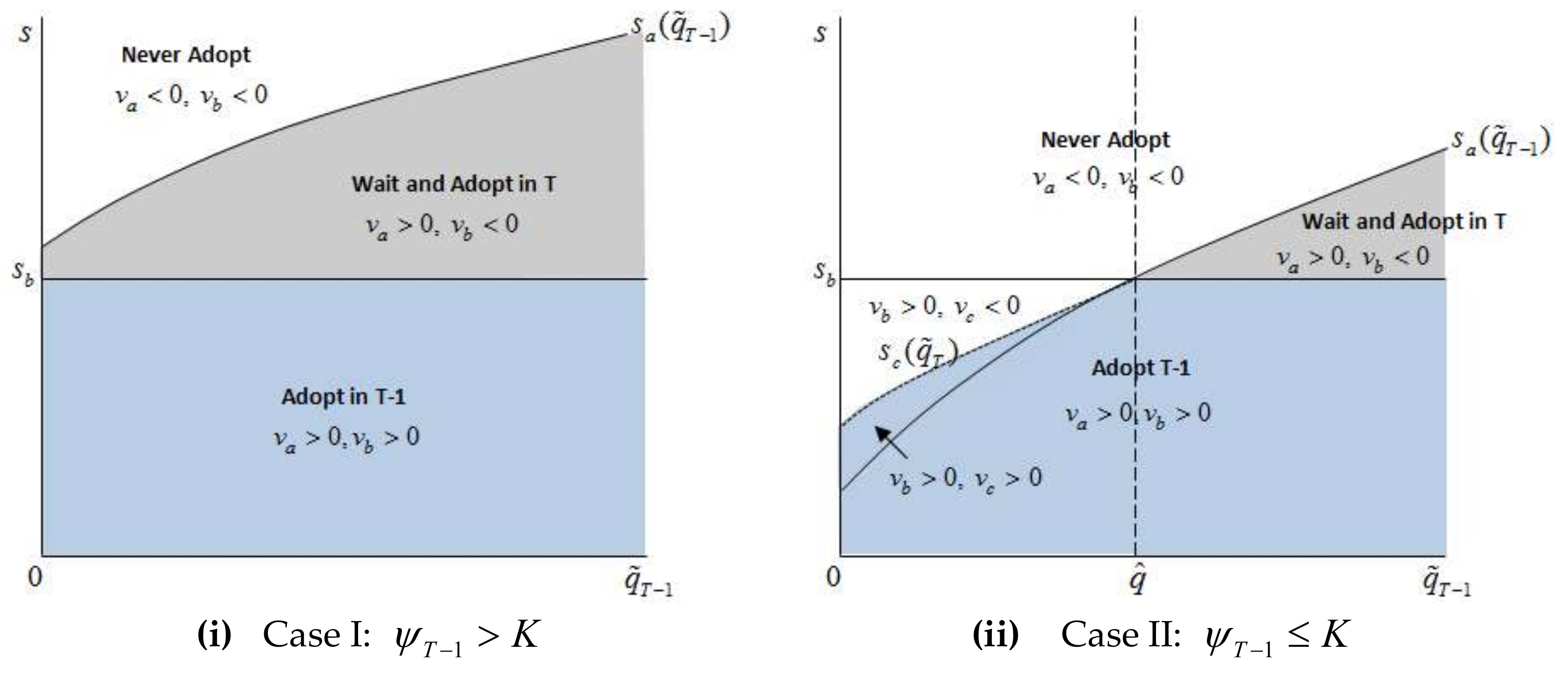
3.1.1. Case I: ${\psi }_{T-1}>K$

In this case, the terminal value $V_T$ is larger than the fixed cost of adoption. This is reasonable when the technology is considered as an optimistic view. We can easily see that $v_a>v_b$, and thus, $s_a({\tilde{q}}_{T-1})>s_b$. The possible values of $s_{T-1}$ for adoption at the beginning of period T − 1 are $s_b$ and below, because $v_a>0$ and $v_b>0$. Then, $v_c>0$, by adoption condition (1). If $v_b$ is negative above $s_b$, we cannot satisfy adoption conditions (1) and (2). From Figure 1a, potential adopters between $s_a({\tilde{q}}_{T-1})$ and $s_b$ will wait and adopt in period T. As ${\tilde{q}}_{T-1}$ increases, we expect that more firms will adopt in the next period. Firms above $s_a({\tilde{q}}_{T-1})$ never adopt the technology. Therefore, the threshold for case I is $s_b$. A firm below $s_b$ will adopt in period T − 1, where the threshold does not depend on ${\tilde{q}}_{T-1}$.

3.1.2. Case II: ${\psi }_{T-1}\le K$

In this case, the terminal value $V_T$ is less than the fixed cost of adoption. Here, there may be a significant investment required to introduce the new technology or a less optimistic view of the technology owing to the high level of uncertainty of the benefit.

When no one adopts in period T − 1, ${\tilde{q}}_{T-1}=0$ and $v_a<v_b$ can be verified easily, in which case $s_a({\tilde{q}}_T)<s_b$. Here, possible values of $s_{T-1}$ for adoption are $s_a({\tilde{q}}_{T-1})$ and below because $v_a>0$ and $v_b>0$, by adoption condition (1). As ${\tilde{q}}_{T-1}$ increases, $s_a({\tilde{q}}_{T-1})$ increases. Then there exists a point where $s_a(\widehat{q})=s_b$ at some critical point $\widehat{q}$, as shown in Figure 1b.

If ${\tilde{q}}_{T-1}<\widehat{q}$, there exists a threshold $s_c({\tilde{q}}_{T-1})$ that is solved for $v_c=0$. Possible values of $s_{T-1}$ for adoption are above $s_a({\tilde{q}}_{T-1})$, where $v_a<0$ and $v_b>0$, and $v_c>0$ can be satisfied to enable adoption in this period using adoption condition (2) (If $v_a\le 0$, the conditions for adopting in period T − 1 are $v_b>0$ and $v_c>0$). Thus, to adopt in this period, the possible values of $s_{T-1}$ should be $s_c({\tilde{q}}_{T-1})$, or below. That is, firms between $s_a({\tilde{q}}_{T-1})$ and $s_c({\tilde{q}}_{T-1})$ will adopt in period T − 1. Firms above the threshold, $\max \left\{s_a({\tilde{q}}_{T-1}),s_c({\tilde{q}}_{T-1})\right\}$, never adopt because the estimated value of adopting in period T is negative ($v_a<0$), regardless of the value of $v_b$. Thus, in the case of ${\tilde{q}}_{T-1}<\widehat{q}$, a firm’s only decision is whether or not to adopt. No firm waits for the coming period to make its adoption decision if the estimated number of adopters will not reach the critical point of $q$. Figure 1b shows there is no area in which firms can wait in this period. Either $s_a({\tilde{q}}_{T-1})$ or $s_c({\tilde{q}}_{T-1})$ is determined by ${\tilde{q}}_{T-1}$. As ${\tilde{q}}_{T-1}$ increases to the critical point $\widehat{q}$, both $s_a({\tilde{q}}_{T-1})$ and $s_c({\tilde{q}}_{T-1})$ increase. Then, more potential adopters will adopt in period T − 1. Thus, the threshold value is $\max \left\{s_a({\tilde{q}}_{T-1}),s_c({\tilde{q}}_{T-1})\right\}$ in the case of ${\tilde{q}}_{T-1}<\widehat{q}$. If the firm’s $s_{T-1}$ is below the threshold, it will adopt. Otherwise, it never adopts the technology because it expects more adopters (at least $\widehat{q}$) for the adoption decision in the next period.

If ${\tilde{q}}_{T-1}>\widehat{q}$, then this case becomes case I. We no longer need $s_c({\tilde{q}}_{T-1})$ to make an adoption decision. The threshold value is $s_b$, as shown in case I, and firms below this threshold will adopt. Although the fixed cost is large, firms between $s_a({\tilde{q}}_{T-1})$ and $s_b$ will wait and adopt in period T. This is because they expect a critical number of adopters in period T − 1, such that it will become sufficiently large to compensate for the fixed costs. Thus, potential adopters expect adoptions in the following period. Firms above $s_a({\tilde{q}}_{T-1})$ never adopt the technology. Figure 1b shows the adoption conditions for Case II. As shown in the figure, the adoption area for case II is smaller than that for case I. Thus, more potential adopters may be pessimistic, owing to huge investments, or they may expect a low relative terminal value owing to the high level of uncertainty related to the benefit. As a different aspect in this case, if the terminal value is too small, the critical point $\widehat{q}$ increases and the tolerance for uncertainty decreases. Then, few or no firms will adopt in this period. However, because the expected number of adopters is larger, the estimated future benefit will be increased by network effects, after which more potential adopters expect to adopt in the next period.

Theorem 1.

There exists a threshold $s_{T-1}^{*}$ for each case, such that if $s_{T-1}<s_{T-1}^{*}$ then the firm adopts; otherwise, the firm never adopts. Here, $s_{T-1}^{*}$ is a non-decreasing function of ${\tilde{q}}_{T-1}$ (See the Appendix A).

• If ${\psi }_{T-1}>K$, $s_{T-1}^{*}=s_b$.
• If ${\psi }_{T-1}\le K$,
  • ${\tilde{q}}_{T-1}<\widehat{q}$, $s_{T-1}^{*}=\max \left\{s_a({\tilde{q}}_{T-1}),s_c({\tilde{q}}_{T-1})\right\}$, and
  • ${\tilde{q}}_{T-1}\ge \widehat{q}$, $s_{T-1}^{*}=s_b$. (same as case I)

3.2. Multi-Period Model

Here, we extend the two-period model above to a multi-period model. In this model, the firm’s choices are slightly different from those of the previous model. In the multi-period model, the possible choices for the adoption decision at some point are adopting, waiting and adopting in the next period, and waiting a few more periods, rather than never adopting.

If the firm adopts the technology in any period t, the value of adoption is given by

$$V{A}_t=[U_t-K]+\delta U_{t,t+1}({\tilde{q}}_t)+{\delta }^2{\psi }_t,$$

where: ${\psi }_t={\delta }^{T-t-1}{V}_T+{\displaystyle \sum _{i=1}^{T-t-1}{\delta }^{i-1}{U}_{t+i+1}(q_{t+i}^{*})}.$

The fixed value of the benefit after adopting in period t is the sum of the discounted value of utility in any subsequent periods and the terminal value in the final period. The value of the utility in subsequent periods is determined by the set of equilibria $q$ for each subsequent period, $\{q_{t+1}^{*},q_{t+2}^{*},\cdots q_{T-1}^{*}\}$, which are found by mapping with $s(q)$ using backward induction through dynamic modeling. The value of non-adoption is

$$N{A}_t=\delta {\pi }_{t+1}(s_{t+1})=\delta \max \left\{V{A}_{t+1},\delta {\pi }_{t+2}(s_{t+2})\right\},$$

where ${\pi }_{t+1}(s_{t+1})$ is the optimal strategy in the coming period, as expressed in Equation (5). The firm will adopt in period t if (i) $V{A}_t>0$ and (ii) $V{A}_t-N{A}_t>0$. Otherwise, a firm may adopt in the next period, or wait a few more periods based on the policy in a proposed model.

Next, we prove how the threshold changes as a function of the risk aversion index of the firm. Let $v_a=V{A}_{t,t+1}({\tilde{q}}_t)=U_{t,t+1}({\tilde{q}}_t)-K+\delta {\psi }_t$, where ${\psi }_t={\delta }^{T-t-1}{V}_T+{\displaystyle \sum _{i=1}^{T-t-1}{\delta }^{i-1}{U}_{t+i+1}(q_{t+i}^{*})}$ is the fixed value of adopting in period t. Then, $U_2,\cdots ,U_T$ are determined by the set of equilibria $q$ for subsequent periods, $v_b=V{A}_t-N{A}_t=U_t-(1-\delta )K$, and $v_c=V{A}_t=[V{A}_t-N{A}_t]+\delta V{A}_{t,t+1}({\tilde{q}}_t)$. In addition, suppose that $s_a$ is a value that solves $v_a=0$, $s_b$ for $v_b=0$, and $s_c$ for $v_c=0$. In each case below, the standard deviation can be a threshold for deciding to adopt in period t.

Using $v_a,v_b,\mathrm{and}{v}_c$, the firm’s adoption conditions in period t are as follows:

• If $v_a>0$, the adoption condition in period t is that $v_b>0$ is sufficient (i.e., adoption condition (ii) is sufficient).
• If $v_a\le 0$, the adoption condition in period t is that $v_b>0$ and $v_c>0$. Thus, conditions (i) and (ii) should both be satisfied before adopting in this period.

Theorem 2.

There exists a threshold $s_t^{*}$ for each case such that if $s_t<s_t^{*}$, then the firm adopts; otherwise, the firm will wait longer or never adopt. Here, $s_t^{*}$ is a non-decreasing function of ${\tilde{q}}_t$ (See Appendix A).

• If ${\psi }_t>K$, $s_t^{*}=s_b$.
• If ${\psi }_t\le K$,
  • $if{\tilde{q}}_t<\widehat{q}$, then $s_t^{*}=\max \left\{s_a({\tilde{q}}_t),s_c({\tilde{q}}_t)\right\}$, or
  • $if{\tilde{q}}_t\ge \widehat{q}$, then $s_t^{*}=s_b$ (same as case I).

When $t=0$, we assume that the initial mean benefit is zero, $\mu =0$, and the standard deviation is the largest value, $s=\overline{s}$, at the beginning of period 0. This is reasonable because firms have no positive signals about the benefit of adoption at this decision point, and so the uncertainty level may be too high without any prior adopters. In addition, the assumption that all buyers have already adopted the technology remains the same.

4. Population Model

The next step is to embed the individual firm’s adoption model into a population model. To begin with, we first model the population of supplier firms as heterogeneous in risk-aversion and identical in all other respects. We further assume that each supplier is linked with all buyers.

We consider a population that is uniformly distributed along an axis $s$, representing the standard deviation of the unknown mean of the belief in period T − 1, $s~[\underset{\_}{s},\overline{s}]$. Analytically, firms at or below a threshold $s^{*}$ will adopt in the period, and firms above $s^{*}$ will wait and either adopt later or never adopt. We define $F(s^{*})$ as the fraction of adopters in the period and $f$ as the density function. The possible number of adopters in the period is at most $\tilde{q}=\lfloor F(s^{*})\cdot N\rfloor$, where $N$ is the population size.

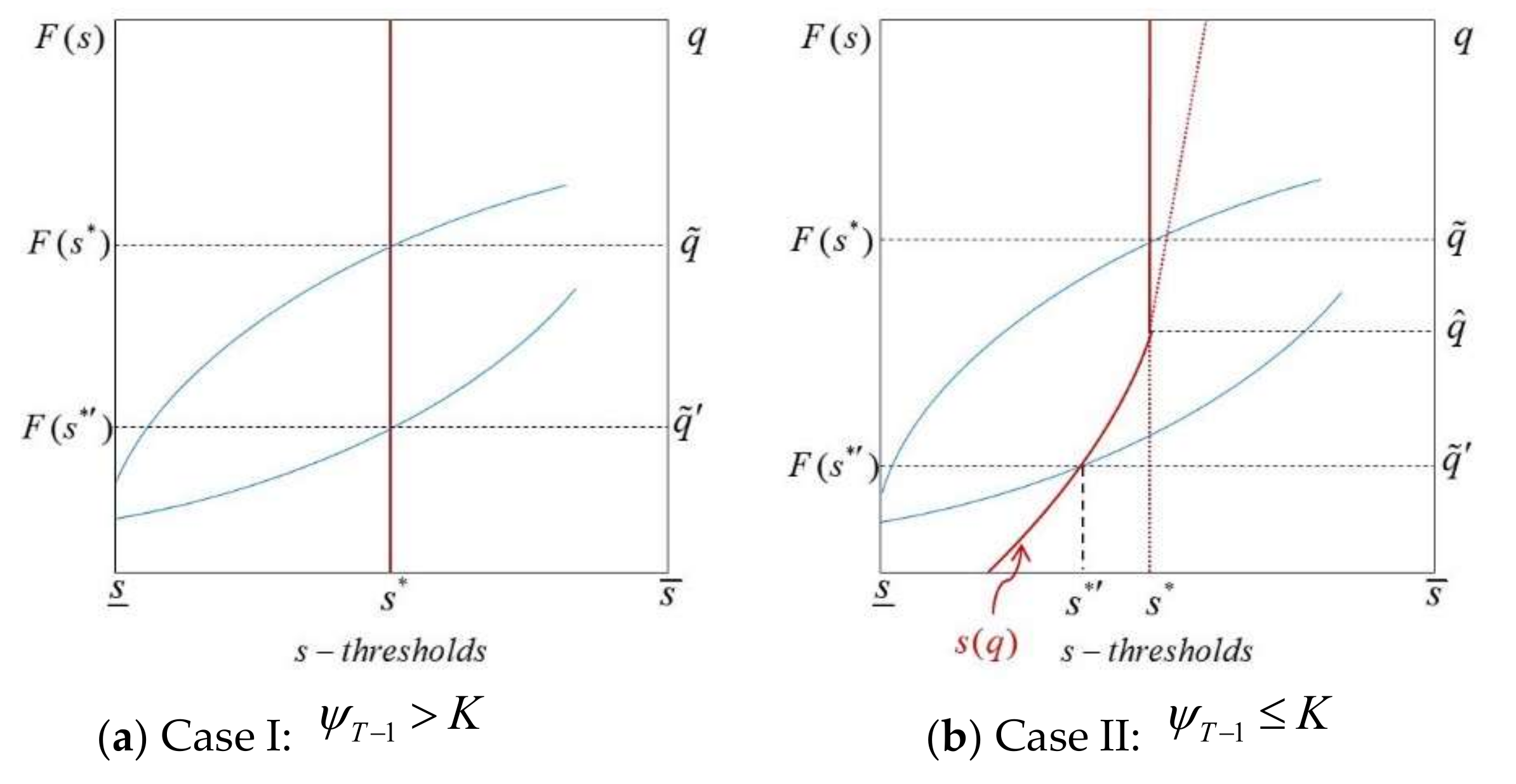
We show that the number of adopters in period T − 1 is a fixed point of the mapping of ${\tilde{q}}_{T-1}$ and $s_{T-1}^{*}$. As shown in Figure 2, $s(\tilde{q})$ is a non-decreasing function in $\tilde{q}$, where $\tilde{q}$ is a discrete variable that increases stepwise by $s(\tilde{q})$. In addition, $F(s)$ is continuous and non-decreasing in $s$. Using graphical observations, we find that cases I and II both have a unique equilibrium of $q$ for any distribution of $s$. As the threshold increases (moves to the right on the horizontal axis), the equilibrium point also increases in both cases. Thus, we prove the following.

In any period, there always exists an equilibrium $q$, which is a fixed point of the mapping of $q$ and $s^{*}$.

Case I. Threshold $s^{*}$ is constant over $q$. As shown in Figure 2, the equilibrium is the point at which $F(s)$ crosses the threshold line. Therefore, there is a unique equilibrium of $q$ for any distribution of $s$.

Case II. The threshold is increasing in $q$ until the critical point of $\widehat{q}$. If a threshold $s^{*}{}^{\prime }$ exists in the interval $[0,\widehat{q})$, a critical point $q$ mapped on the curved threshold level $s(q)$ is less than that on the straight threshold level $s^{*}$ (${\tilde{q}}^{\prime }<\tilde{q}$), as shown in Figure 2. For $\widehat{q}$, the threshold is constant, as case I. Therefore, there is a unique equilibrium $q$ for any distribution of $s$.

This is very important, because we can determine $s$ based on this fixed point $q$ across periods. That is, in each period, a critical level on the risk aversion index exists, such that all firms at or below that level will adopt the technology, and all firms above that level will choose to wait rather than adopt. This allows us to derive an adoption curve in terms of the accumulated fraction of firms that have adopted the technology in or before any given period. Supposing $A_{\tau },\tau \in \{T-1,T\}$ is the fraction of adopters in period $\tau$, $\{A_{T-1},A_T\}$ represents an adoption curve in a two-period model as a cumulative distribution function. We extend the model to a multi-period model. We also consider the case in which there is a cost for observing information, as well as the possibility that the information is not truthful.

In the following section, we show how to compare any two adoption curves using numerical experiments such that one denotes faster adoption than the other.

5. Numerical Analysis of the Model

The set of experiments focuses on how the adoption curve of the two-period model changes with different parameters. There are at least two important metrics inherent in the adoption curve: the fraction of the total population that joined in both periods, and the percentage of these that were early adopters. These metrics provide the coverage and the speed of adoption, respectively. Here, we examine what happens to the adoption curve in a series of scenarios.

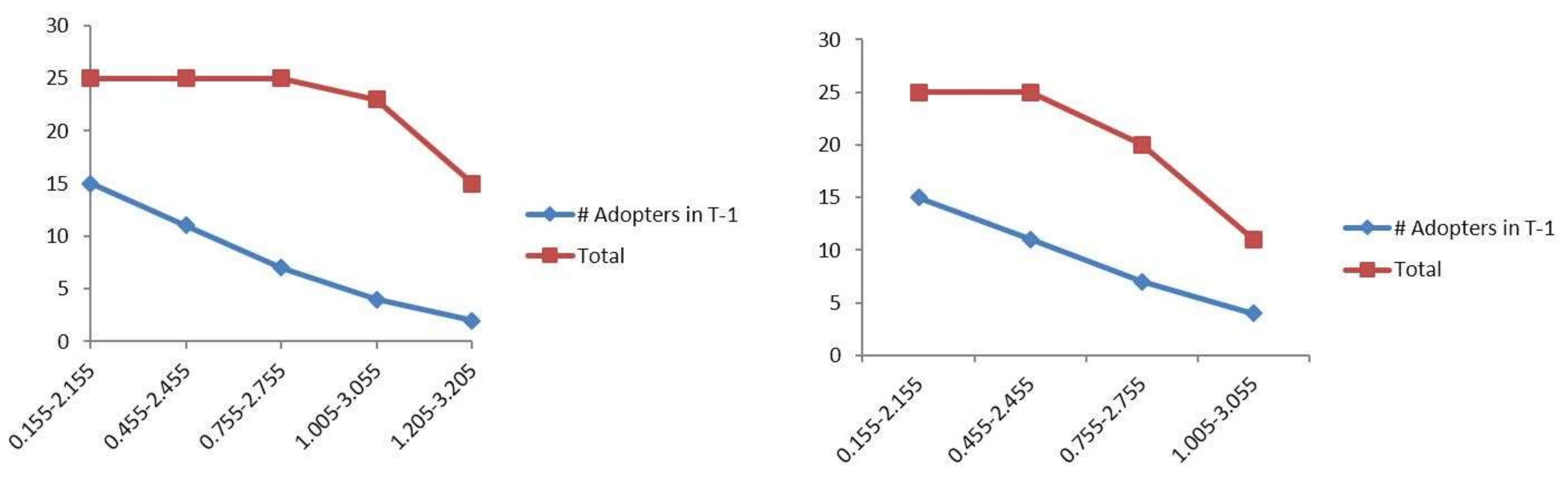
We begin by considering three cases of the spread of the population along the s-axis. First, we examine the effect on the adoption curve with different ranges of the population scale and with the same $\underset{\_}{s}$. If firms in a population spread within a small range of the population scale with the same $\underset{\_}{s}$, these firms are more willing to take the risk than are those that spread within a large range, because a smaller s denotes a greater number of risk-takers. Based on our numerical experiment, if the spread of the population increases, the number of adopters decreases across periods in both case I ($V_T>K$) and case II ($V_T<K$) as shown in Figure 3. Second, we examine the effect on the adoption curve when the range of the population scale remains the same, but the means of s vary. That is, each population group has different values of $\underset{\_}{s}$ and $\overline{s}$. The results show that if the mean of s increases, the number of adopters decreases across periods in both cases as shown in Figure 4. Lastly, we test the effect of populations with different scales, but with the same mean s. That is, each population group has different $\underset{\_}{s}$ and $\overline{s}$, but all have the same mean s. If a population has a smaller $\underset{\_}{s}$, then it has a larger $\overline{s}$. In contrast, if a population has a larger $\underset{\_}{s}$, then the range of the scale is smaller because it must have a smaller $\overline{s}$ in order to have the same mean s. The results show there is no effect on the two adoption curves.

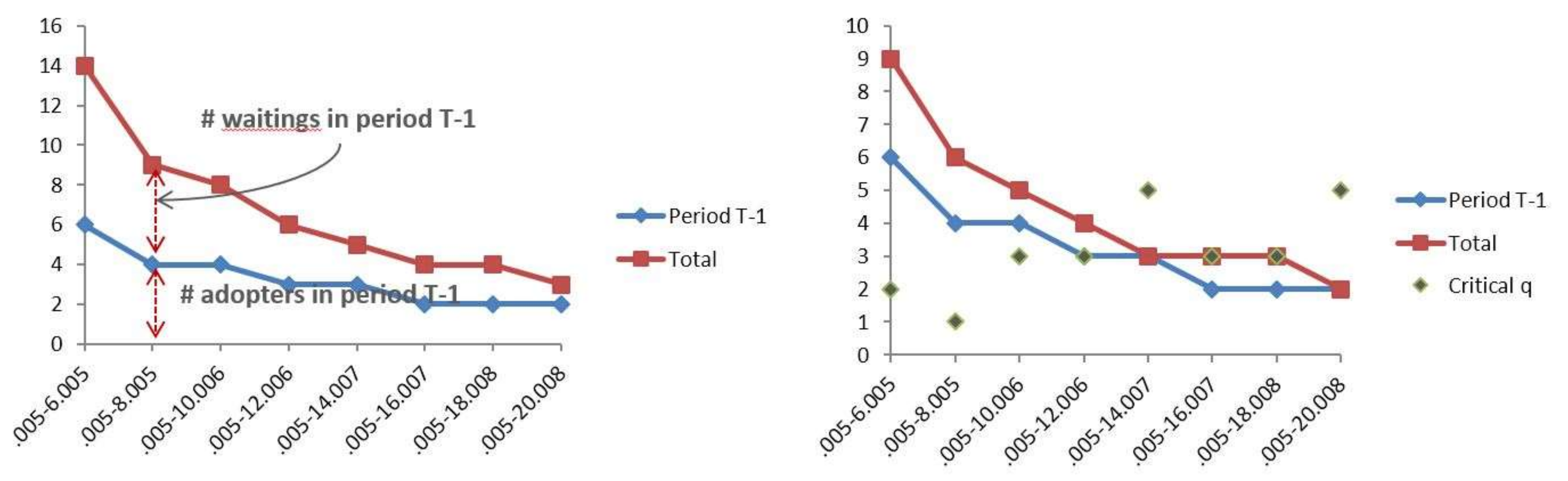
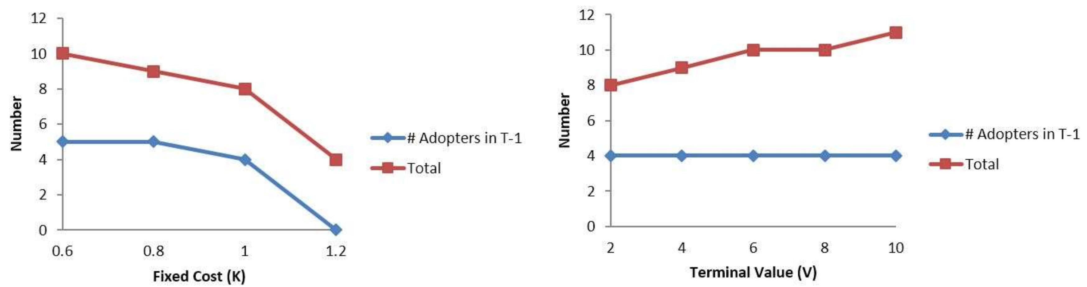
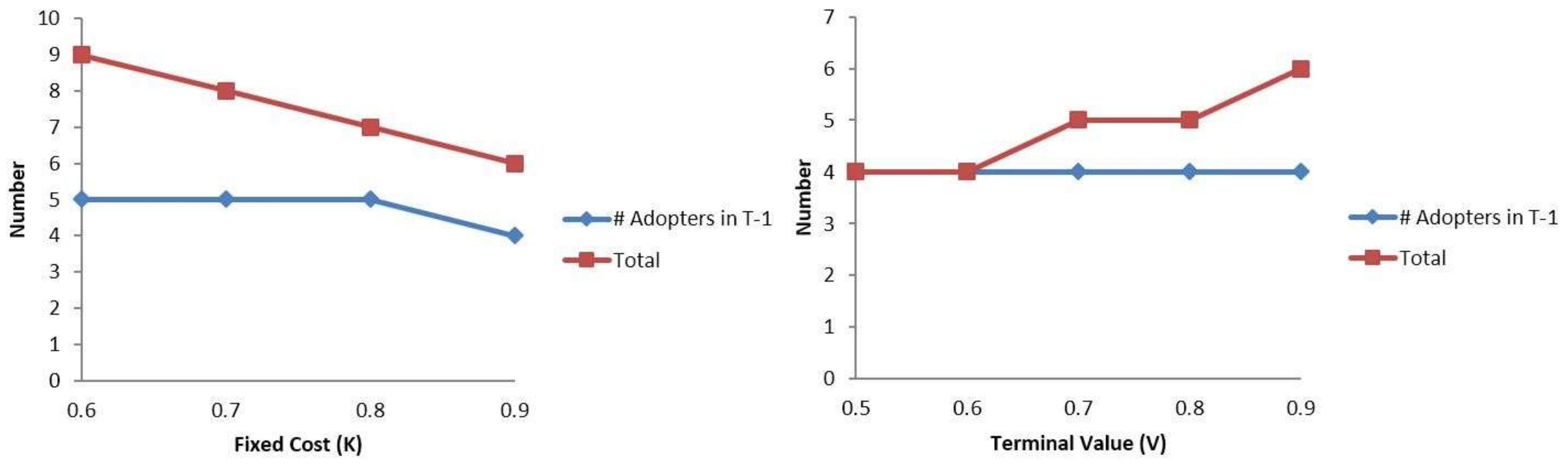
Second, we test the effects of fixed adoption costs and terminal values in the finite-horizon model. The results are shown in Figure 4, Figure 5 and Figure 6. As the adoption costs increase with fixed terminal values, the number of adopters decreases across periods, and the number of firms waiting in period T − 1 decreases in both cases. As the terminal values increase with fixed costs, the number of adopters in period T − 1 does not change across periods. However, the number of firms waiting in period T − 1 increases in both cases. As a result, the total number of adopters in the population increases.

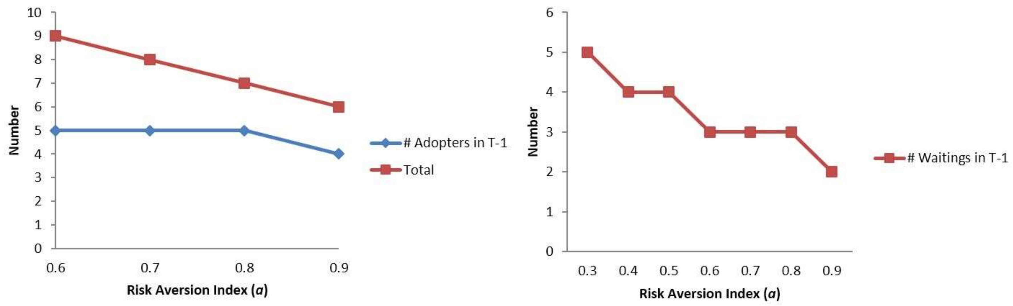
Third, the type of risk aversion affects the adoption rates of the technology significantly. Firms with a lower degree of risk aversion are more optimistic in terms of adopting the technology. In contrast, those with a higher degree of risk aversion are more pessimistic, and so are less willing to adopt or would prefer to wait. As shown in Figure 7, as the risk aversion index increases, the number of firms that wait in this period and that will adopt in the next period decreases. Therefore, the total number of adopters in the population decreases.

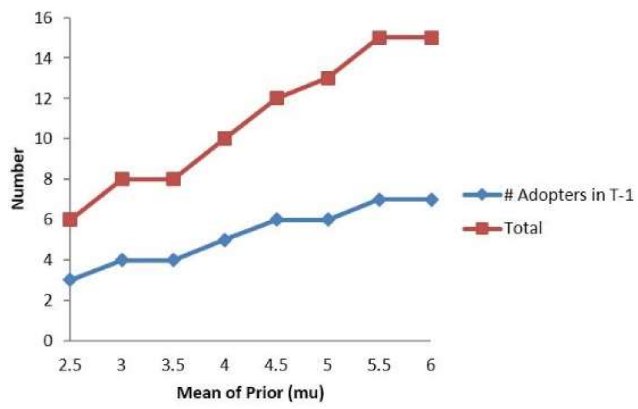
Fourth, we examine the effects of the prior mean of the benefit of adoption. As the mean increases, both the number of adopters and the number of firms waiting in period T − 1 increase. Therefore, the total number of firms that wait also increases, as shown in Figure 8.

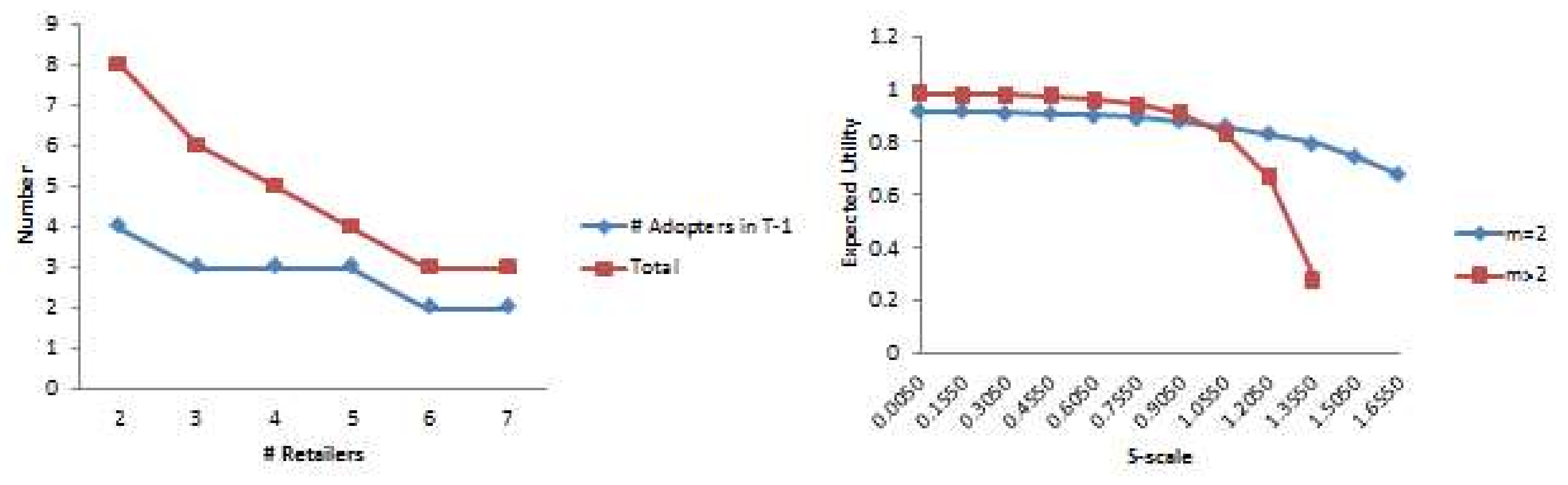
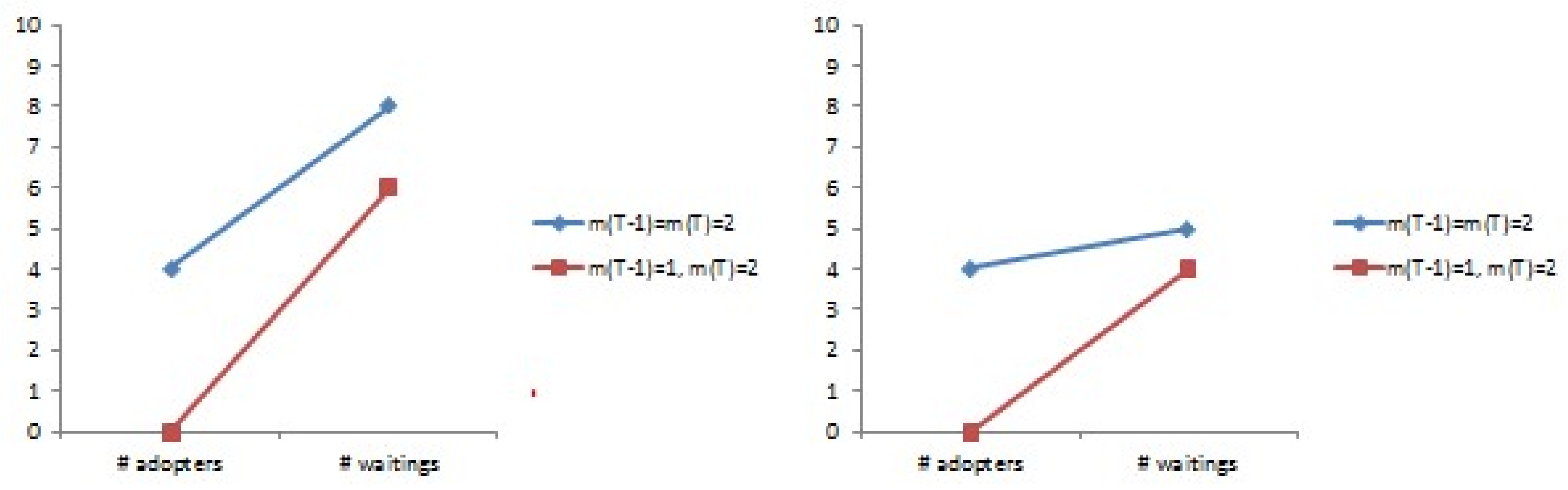
Lastly, we consider the effect of the adoption patterns in the other population group, that is, the effects of buyers’ behavior in the two-level supply chain. We consider two scenarios: the effect of the number of prior adopters in a buyer population, and the adoption speed in a buyer population. First, as the number of adopters in a buyer population increases, both, the number of adopters and the number of firms that choose to wait in period T − 1, decreases. This is counterintuitive. Since we may expect buyer firms that have adopted to stimulate suppliers to adopt the technology, the effect of the number of buyers that have adopted should be positive in the rate of adoption in the supplier population.

The results of this experiment show that a supplier’s expected utility decreases on the s-axis for both tests. In the first case, there are two adopters in the buyer population. In the second, there are at least three adopters in the buyer population. The higher the degree of risk faced by a firm, the lower is its expected utility. That is, firms that face greater risk are not affected by the number of buyers that have already adopted in the past. Rather, the effect of such firms is negative. We next examine the case of buyers adopting slowly, for example, some buyers adopt at the beginning of the period, and the remainder adopt in period T. This is known to suppliers. We numerically test the effect of buyer adoption speed using two test groups. In the first, all buyers have already adopted before processing the model. In the second, some buyers adopt in the next period, which is determined exogenously, by our assumption. The results show that in the first case, more suppliers adopt in the next period, even though there, we have the same number of adopters in the first period for case I ($V_T>K$) and case II ($V_T<K$). See Figure 9 and Figure 10.

6. Conclusions

In this study, we develop a model to analyze inter-organizational technology adoption in a supply chain. To develop the dynamic mechanism that influences the level of uncertainty, we model a firm’s adoption decision as a dynamic program. The state space in each period includes the firm’s prior belief distribution, which depends on the number of suppliers and buyers that have already adopted the technology. The action space includes adoption or non-adoption in this period. As more firms adopt, the information they provide reduces the uncertainty related to the adoption benefits via network effects.

Based on the suggested finite-horizon dynamic formulation, we develop a population model that includes heterogeneity in the population to capture the factors affecting the speed of diffusion. This allows us to derive an adoption curve that is specified by the accumulated fraction of firms that have adopted the technology in or before any given period. Using numerical experiments, we use the population model to consider the effect of several strategies observed in practice. We also discuss the conditions under which such an action is useful to the firm. First, in practice, technology in a supply chain is often adopted by large retailers (buyers), which then mandate that suppliers do so as well. For example, in recent years, several large retailers and government agencies have required that suppliers label shipments with RFID tags. In this case, the choices available to a supplier are to adopt the technology or to stop being a supplier or partner. That is, the market power of the mandating entities is such that suppliers overwhelmingly comply with the requirement. However, such mandates may stimulate the speedy diffusion of the technology within a supply chain. We capture this in our model using combinations of numbers of buyers and suppliers that have adopted at time zero or at an earlier time. We also provide insight into the combinations and the timing of mandated adoption that are effective in achieving a faster adoption curve. Second, many firms invest in pilot programs to better estimate the benefit of adopting a technology. Here, a small proportion of firms are part of a pilot testing stage. Interestingly, many firms in this case research the potential of the technology and consider being part of the pilot program in order to reduce the uncertainty related to the benefits of adoption. Here, we analyze the effect of pilot testing on the adoption curve by introducing another possible action for the firm, that is, a reduction in the standard deviation of the prior can be obtained at a fixed cost.

The first limitation of this study is that we restrict our analysis to a two-level supply chain only, and do not develop the model precisely for extended cases. Other scenarios that can be examined in future research include the following: (1) a buyer is dominant; (2) a supplier is dominant; and (3) the supply chain system is under centralized control. Furthermore, a game-theoretic approach can be used to determine an equilibrium strategy for the adoption decision under each scenario. Second, the proposed model describes a simple per-period cost-benefit utility function for the adoption of a new inter-organizational technology. A more explicit structure used to explain the benefits and costs of adoption will enable a more precise technology adoption model. Lastly, we consider only costless information from previous adopters within the same population group. However, firms receive information from various sources, including adopters within the same group, and may pay significant costs for such information. In this case, the model will change significantly if we consider the weighted value of information instead of the amount of information. These issues can be resolved by developing a model based on economic theory.