Implementation of Observed Sky-View Factor in a Mesoscale Model for Sensitivity Studies of the Urban Meteorology

Abstract

The sky view factor (SVF) is an important radiometric parameter for assessing the canopy energy budget of urban areas. There are several methods to determine the SVF observationally. The most common is taking a photo with a digital camera equipped with a fish-eye lens and then converting ratio of sky area to canopy area into SVF. However, most urban canopy models use this variable as derived from idealized canopy geometry. To evaluate the effect of inputting observed SVFs in numerical models, we evaluated a mesoscale model’s performance in reproducing surface wind and surface temperature when subjected to different ways of SVF prescription. The studied area was the Metropolitan Area of São Paulo (MASP) in Brazil. Observed SVFs were obtained for 37 sites scattered all over the MASP. Three simulations, A, B, and C, with different SVF and aspect-ratio prescriptions, were performed to analyze the effect of SVF on the urban canopy parameterization: Simulation A (standard) used the original formulation of the Town Energy Budget (TEB) model, computing the SVFs from the aspect-ratios; Simulation B used the observed SVFs, but keeps aspect-ratios as original; and Simulation C used the aspect-ratios computed from observed SVFs. The results show that in general inputting observed SVFs improves the model capability of reproducing temperature at surface level. The comparison of model outputs with data of regular meteorological stations shows that the inclusion of observed values of SVFs enhances model performance, reducing the RMSE index by up to 3 ${}^{\circ }$C. In this case, the model is able to better reproduce the expected effects in the wind field, and consequently the temperature advection, of the urban boundary layer to a large urban area. The result of Simulation C shows that the surface wind and temperature intensity for all urban types is higher than those of Simulation A, because of the lower values of the aspect ratio. The urban type with high density of tall buildings increase up to 1 $\mathrm{m}{\mathrm{s}}^{-1}$ in the wind speed, and approximately 1 ${}^{\circ }$C in temperature, showing the importance of a better representation of the urban structure and the SVF database improvement.

1. Introduction

Today, more than 50% of the world population lives in urban areas, and, in Brazil, this fraction is higher than 80% [1]. This makes the knowledge of the urban climate important information for society. Besides the economic role, it is important to study the influence of the urban environment on people’s quality of life and materials to subsidize mitigating actions of the negative effects that the urban climate may have on people. The investigation of the urban climate in recent years has spent a considerable effort in developing numerical models to simulate the properties of the urban boundary layer, in parts motivated by the lack of adequate time and spatial resolution of observations needed for applications in environmental management, weather, and climate forecasting.

Many numerical models represent urban regions through street canyons elements [2,3,4], which consist of two parallel columns representing buildings on both sides of a street. Such representation of the urban surface can account for the distribution of momentum sinks in all canyon elements (roof, walls, and street), as well as the radiation shadowing effects over the street and walls, and the radiation trapping through multiple reflections by the walls. Some research has used mesoscale numerical models coupled with urban landscape parameterizations to improve model performance in urban areas or to assess the urban aspect-ratio obtained with algebra form factor (Equation (3)) to study heat island [5,6,7,8]. An important variable that defines the urban structure in those schemes is the Sky-View Factor (SVF). It has also been used to describe the urban geometry [9,10]. By definition, SVF is the ratio of the radiation received (or emitted) by a planar surface to the radiation emitted (or received) by the entire hemispheric environment [11,12]. For practical purposes, it can be regarded as the ratio of solid angle occupied by the sky from a given viewpoint to the whole hemispheric solid angle (2$\pi$). In the overwhelming majority of the cases of interest, such a viewpoint is on a wall or street surface. The aspect-ratio (defined as the ratio of building height to the street width), therefore related to the SVF, has influence in the generation and the urban heat island intensity [13], as it contributes to a decrease in the long-wave radiation emission from the canyon. As a result, there is a correlation between the surface temperature and SVF [14]. In addition, the evolution of the temperature follows a similar pattern of the sensible heat flux with respect to the SVF, with a decrease as the aspect-ratio increases during the day [15]. The canopy energy budget in urban areas is a whole subject in urban climate studies and can vary significantly from one neighborhood to another, also influencing atmospheric dispersion [16,17]. The canopy energy budget is strongly affected by the aspect-ratio either because it changes the local radiation absorption by the street and walls or because it impacts the wind circulation [18,19]. It is worth mentioning that the canopy energy budget drives the diurnal cycle of the boundary layer process by altering momentum and heat exchanges between atmosphere above and the surface layer [20]. In particular, the whole urban boundary layer can be impacted by changes of the aspect-ratio [15].

A planned combination of suitable aspect ratios and canyon orientation can also improve thermal comfort at pedestrian level [21]. A positive correlation between normalized air temperatures and the aspect-ratio for uniform surface heating is found [22]. Thus, it becomes apparent that the aspect-ratio can impact the surface and air temperatures and, consequently, the energy fluxes inside the urban canyon. The spatial average of SVF values has a close negative relationship with daytime intra-urban temperature differences, indicating that SVF is a significant factor for understanding the microthermal climate of a region [23].

Generally, mesoscale models use schemes that present the SVF as a numerical solution of a radiation transfer relationship between two surfaces [24], with a general model for the buildings, as a form factor. Therefore, this paper aims to improve the representation of the urban morphology inside the urban parametrizations in mesoscale models, by using SVF observations. It is important to emphasize that this study tried to show the improvement of the use of a real SVF, instead of the form factor calculated by numerical approach for the Metropolitan Area of São Paulo (MASP), a complex urban region that consists of 39 municipalities totalling over 20 million inhabitants, covering an area of approximately 8000 km${}^2$, and located in a large area of complex topography, 60 km from the Atlantic Ocean.

2. Methodology

2.1. Sky-View Factor

There are several methods to obtain the SVF. The most common is taking a photograph with a camera equipped with a fish-eye lens [25,26,27,28]. In this work, the method proposed by Santos et al. [29] was employed using this kind of photographs. This method is simple, easy-viewing and handling because it uses CAD (Computer-Aided Design) and GIS (Geographic Information System) software for mapping the visible sky and calculates the SVF.

Obtaining SVFs for several points in an urban region such as the MASP is very difficult due to chaotic traffic and size of the area to be sampled. Thus, the urban landscape was classified via satellite images by selecting four different urban types [30,31] to represent the differences between urban regions in MASP (Figure 1). The information about the different urban types was obtained based on the CBERS-2B satellite image (China–Brazil Earth Resources Satellite), using the maximum likelihood classification method. The type called urban 1 is considered the center of the city, with the high density of tall buildings and large avenues with intense vehicular traffic. Urban 2 type is located in the vicinity of this central region and is characterized by high density of buildings, but with a mixture of medium-sized buildings. Urban 3 type has a more residential characteristic with lower buildings (1–3 floors) and narrow streets, while the suburban type, situated on the outskirts of the urban area, is the transition between the urban and the rural land use.

The use of “urban-types” criterion instead of the local climate zones (LCZs, [32]) is due to the fact that the first is used for setting up the model urban surface configuration. This configuration has been used in several investigations in MASP by other researchers [6,31,33,34]. Thus, for the sake of consistency and comparability with previous works, we kept the urban classification system as it was originally programmed in the model, although the parameter values can be changed. Despite the use of that urban-type classification system, there is an approximate equivalence with the LCZ classification. For instance, by comparing values of aspect-ratio and building height in Table 2 with those in Stewart and Oke’s Table 3 [32], we have found that, for the types urban 1, 2, 3 and suburban, the approximate LCZs would be, respectively, 1, 2, 3 and something between 5 and 6.

The obtaining of SVF was focused mainly in the São Paulo city, where the four types of urban land use considered in this study coexist. Figure 2 shows the 37 chosen points where the SVF were obtained based on equidistant projection [29]. The photos were taken with a digital camera and a fish-eye lens in the chosen points considering the ease and safety to settle the camera on the street. The SVF values were identified for each urban type in the MASP, performing an average of the same. The value obtained will be considered as representative of that type of urban land.

2.2. Modeling System

To study the effects of the implementation of SVF to represent urban morphology on mesoscale models, the BRAMS model (Brazilian Developments on the Regional Atmospheric Modeling System [35,36]) was used. The code and users guide of all versions of the model are available on the BRAMS website (http://brams.cptec.inpe.br). This is a mesoscale model that was modified to represent tropical and sub-tropical atmospheric processes. It includes various physical parameterizations of turbulent mixing, convection, radiation and surface processes. In this work, we used BRAMS version 4.2.

BRAMS includes the LEAF (Land Ecosystem–Atmosphere Feedback) surface–vegetation– atmosphere transfer module, which provides lower boundary conditions necessary to the atmospheric model [37,38]. Assuming that the horizontal flows between the different types of surfaces in a grid cell are small compared to vertical flows, LEAF allows the subdivision of each cell on different types of surfaces, called patches [38]. These patches are intended to represent variations in surface characteristics (soil type, moisture, slope, vegetation type, and water bodies). The prognostic equations are resolved for each patch on the grid cell. In this approach, all patches interact with the same column of air, according to the fraction of the surface type.

The Town Energy Budget scheme (TEB; [4]) was run together with LEAF for the cases of urban patches. The simplicity of representing the urban canyon with infinite length, as TEB does, allows us to write the SVF as two-dimensional equations. The street and wall SVF are written in the TEB scheme, respectively, as

$$\begin{array}{cc}\hfill {\psi }_s& ={(a_r^2+1)}^{1/2}-a_r\hfill \end{array}$$

(1a)

$$\begin{array}{cc}\hfill {\psi }_w& =\frac{1}{2}\left(\frac{1-{\psi }_s}{a_r}\right)\hfill \end{array}$$

(1b)

where $a_r$ is the urban canyon aspect-ratio, defined as the ration between construction height and width $(h/w)$.

To consider the effect of vegetation in urban areas, a weighting average of turbulent fluxes is performed [33]:

$${\varphi }_{ij}=(1-\gamma ){\varphi }_{urb}+\gamma {\varphi }_{veg}$$

(2)

where ${\varphi }_{urb}$ and ${\varphi }_{veg}$ are heat and momentum turbulent fluxes for urban and vegetated region, respectively; ${\varphi }_{ij}$ is the total flux at the grid point $(i,j)$; and $\gamma$ is the fraction of the urban vegetation grid point obtained from NDVI (Normalized Difference Vegetation Index) data. Previous numerical simulations showed that increasing the vegetation fraction in the whole MASP by 25% could increase the latent heat flux by up to 280 $\mathrm{W}{\mathrm{m}}^{-2}$, while the sensible heat flux decreases by up to 200 $\mathrm{W}{\mathrm{m}}^{-2}$ [31]. For simulated scenarios, it was shown that when the larger the vegetated fraction, the atmosphere becomes closer to stable conditions.

2.3. Simulations Description

The characteristics and parameterizations used in the numerical model are presented in

Table 1. Parameterizations and options used in the experiments.

Nudging points in lateral boundary region	5
Nudging time scale at lateral boundary	3600 s
Nudging time scale at top boundary	1800 s
Lateral Boundary Condition	Klemp [40]
Short and long wave Parameterization	Chen and Cotton [41]
Frequency of radiation tendency update	1800 s
Number of soil layers	4 (−2.0, −1.5, −0.25 and −0.05 m)
Soil saturation degree	0.49, 0.44, 0.42, 0.35
Turbulence Parameterization	Anisotropic deformation Smagorinski [42] with formulations by Hill [43] and Lilly [44]

[6], and some of the parameters used in the TEB scheme for each type of use of urban land and their respective vegetation is presented in

Table 2. Values of some parameters used in the simulations for TEB.

Parameters	Urban 1	Urban 2	Urban 3	Suburban
Roof Albedo	0.18	0.18	0.18	0.18
Street Albedo	0.08	0.08	0.08	0.08
Wall Albedo	0.14	0.14	0.14	0.14
Roof Emissivity	0.9	0.9	0.9	0.9
Street Emissivity	0.95	0.95	0.95	0.95
Wall Emissivity	0.9	0.9	0.9	0.9
Aspect-Ratio	10	2	1.25	0.6
Building Heights (m)	50	20	10	5
Roughness Length (m)	3	2	1	0.5
Traffic Sensible Heat Flux ($\mathrm{W}{\mathrm{m}}^{-2}$)	90	60	60	10
Traffic Latent Heat Flux ($\mathrm{W}{\mathrm{m}}^{-2}$)	10	10	5	5
Industrial Sensible Heat Flux ($\mathrm{W}{\mathrm{m}}^{-2}$)	14	14	10	10
Industrial Latent Heat Flux ($\mathrm{W}{\mathrm{m}}^{-2}$)	50	50	30	30
Urban Fraction	0.7	0.6	0.5	0.5
Vegetation Type	Short Grass	Mixed Forest	Evergreen broadleaf tree	Short Grass

. The vegetation type was based on the Environmental Atlas of São Paulo [39].

For initial and boundary conditions, the analyses of Global Forecasting System (GFS) with 1${}^{\circ }$ of horizontal grid spacing, provided by the National Center for Environmental Prediction (NCEP), were used. All simulations were run for 72 h, starting from 00Z of 17 July 2008, corresponding to a period of clear days. Two nested grids were used (Figure 3), and the horizontal grid spacing (from the lower to the higher resolution) was 16 km and 4 km. This horizontal grid spacing is considered adequate due to the number of SVF data used. For topographical data, the US Geological Survey files, with the spatial grid spacing of 1 km, were used. To obtain the vegetation fraction, NDVI data from the MODIS sensor from AQUA/TERRA satellite for 18 July 2008, with 250 m resolution, were used.

From those 37 SVF obtained, average values were calculated for each urban type (1–3) and suburban. Afterwards, these values were inserted into the BRAMS model.

As an initial evaluation, three simulations were performed to analyze the impact of SVF on the urban canopy parameterization:

(i)

Simulation A used the original formulation of the TEB scheme, in which the fundamental canopy geometric variable is the aspect-ratio, as given according to the urban-type classification (Table 2). From the aspect-ratio, the street and walls sky-view factors were computed using the mathematical formulation of the model (Masson’s TEB). In other words, Simulation A was the standard simulation.

(ii)

Simulation B used the observed street SVFs for each grid-point on the surface instead of computing them from the aspect-ratio. Wall SVF was obtained from Equation (1a). Thereby, the entire canopy radiation budget is now geometrically ruled by observed SVFs, but not by the aspect-ratios. The aspect-ratios, however, play their role in other aspects of the model dynamics such as scaling the roughness length and influencing the momentum sink.

(iii)

Simulation C used the street and wall SVFs as in Simulation A, but the aspect-ratios was computed as a function of the observed street SVF, according to

$$a_r=\frac{h}{w}=\frac{1-{\psi }_s^2}{2{\psi }_s}$$

(3)

Thus, Simulation B can be considered a sensitivity test for the effect of SVF on the net radiation budget for each urban area. Consequently, it influenced the surface energy budget.

To evaluate the model, statistical indexes were calculated using surface data from meteorological stations spread over the MASP.

Table 3. Location of the surface stations in the MASP.

Surface Station	Latitude	Longitude	Altitude
São Caetano	23${}^{\circ }$36${}^{\prime }$10${}^{\prime }$${}^{\prime }$ S	46${}^{\circ }$34${}^{\prime }$29${}^{\prime }$${}^{\prime }$ W	740 m
Guarulhos Airport (METAR)	23${}^{\circ }$26${}^{\prime }$00${}^{\prime }$${}^{\prime }$ S	46${}^{\circ }$28${}^{\prime }$00${}^{\prime }$${}^{\prime }$ W	751 m
Congonhas Airport (METAR)	23${}^{\circ }$38${}^{\prime }$03${}^{\prime }$${}^{\prime }$ S	46${}^{\circ }$38${}^{\prime }$59${}^{\prime }$${}^{\prime }$ W	802 m
Mirante do Santana (INMET)	23${}^{\circ }$29${}^{\prime }$47${}^{\prime }$${}^{\prime }$ S	46${}^{\circ }$37${}^{\prime }$12${}^{\prime }$${}^{\prime }$ W	792 m
IAG	23${}^{\circ }$39${}^{\prime }$04${}^{\prime }$${}^{\prime }$ S	46${}^{\circ }$37${}^{\prime }$21${}^{\prime }$${}^{\prime }$ W	799 m

lists all surface stations used to evaluate the model.

Temperature and specific humidity taken at 2 m agl were used for sake of validation, using root mean square error ($RMSE$), bias [45] and Pielke index ($D_{Pielke}$) [46], which considers the Pielke model skill definition [47] as presented in Equation (4):

$$D_{Pielke}=\left|1-\frac{{\sigma }_s}{{\sigma }_o}\right|+\frac{RMSE}{{\sigma }_o}+\frac{RMS{E}_{BIAS}}{{\sigma }_o}$$

(4)

where $\sigma$ is the standard deviation and indexes s and o indicate simulation and observation, respectively. The model skill is shown if $D_{Pielke}<2$, and the lower is $D_{Pielke}$, the better is the simulation result. For the case of perfect simulation, $D_{Pielke}$ is equal to 0. $RMS{E}_{BIAS}$ is the $RMSE$ removing a constant $BIAS$ combined to model’s tendency.

3. Results and Discussion

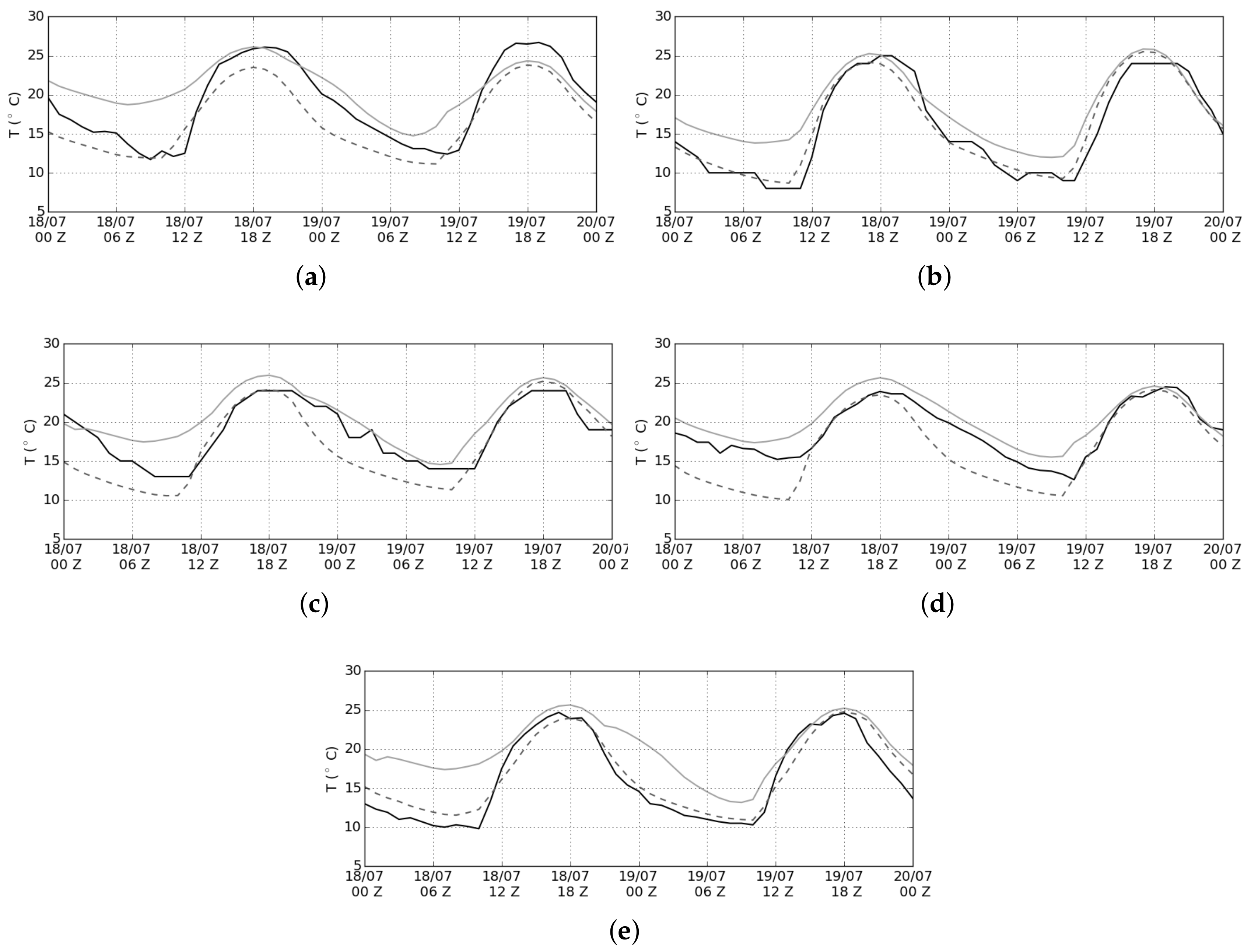
The SVF implemented in the model were calculated from 37 photos. Figure 4 shows two examples of these photos obtained for the sites 1 and 37, corresponding to high (Figure 4a) and low (Figure 4b) aspect-ratios, respectively.

Table 4. Sky-View Factor values used at studied sites.

Site	SVF	Site	SVF	Site	SVF
1	0.6161	14	0.8612	27	0.6539
2	0.4286	15	0.6889	28	0.8218
3	0.6687	16	0.1816	29	0.8077
4	0.7309	17	0.6618	30	0.5846
5	0.6939	18	0.8327	31	0.7707
6	0.9204	19	0.5482	32	0.8394
7	0.5732	20	0.5391	33	0.8508
8	0.5613	21	0.8052	34	0.7994
9	0.9098	22	0.8270	35	0.7506
10	0.8071	23	0.7886	36	0.6179
11	0.7355	24	0.5771	37	0.8176
12	0.7980	25	0.7036
13	0.9126	26	0.6201

presents the SVF obtained for all 37 sites. The SVF values range from 0.18 to 0.92, showing large differences among sites, as expected. The sample standard deviation are 0.10, 0.17, 0.07, and 0.09 for urban type 1, 2, 3, and suburban, respectively. The values of SVF also present a large variability as a result of the difference among regions in MASP, illustrated in Figure 4.

The average SVF values for each urban type were calculated from data presented in Table 4 and are presented in

Table 5. Average SVF obtained with a digital camera equipped with fish-eye lens (Observed), standard deviation, N is the number of data, SVF obtained from Equation (1a) (Numerical) for each urban type and $a_r$ is the aspect-ratio obtained with algebra form factor [Equation (3)].

Urban Type	Observed SVF	Standard Deviation	N	Numerical SVF	${\mathit{a}}_{\mathit{r}}$
Urban 1	0.62	0.10	5	0.05	0.50
Urban 2	0.68	0.17	19	0.24	0.40
Urban 3	0.79	0.07	10	0.35	0.24
Suburban	0.83	0.09	3	0.57	0.19

. These values are compared with those calculated from the Equation (1a) for aspect ratio values listed in Table 2. The modeled SVF are much lower than those obtained empirically for all urban types, due to the aspect-ratio values used in the simulations (Table 2). The largest discrepancy occurs in sites type urban 1, where modeled form-factor value is less than 10% of the observed one. These observational data were inserted into the model, by modifying its code, to try better representing the structures of each urban type in comparison with the numerical values and to evaluate the influence of SVF in the simulated temperature.

3.1. Evaluation

For the analysis, the first 24 h of simulations were ignored to avoid spin-up effect [48]. Figure 5 shows the evolution of the air temperature at 2 m for all stations. Evaluation indexes are shown in

Table 6. Statistical air Temperature indexes calculated from Simulations A and B, from the observations at 2 m agl.

	Simulation A			Simulation B
Station	BIAS	RMSE	${\mathbf{D}}_{\mathit{PIELKE}}$	BIAS	RMSE	${\mathbf{D}}_{\mathit{PIELKE}}$
São Caetano	1.85	3.44	1.65	−1.24	2.78	1.02
Guarulhos	2.44	3.28	1.16	0.21	1.43	0.52
Congonhas	1.93	2.50	1.19	−1.69	2.38	1.17
Mirante	1.55	1.89	0.99	−2.40	3.20	1.95
IAG	3.85	4.67	1.71	0.65	1.59	0.69

. The inclusion of SVF in the subroutine TEB of the BRAMS improved the model capability of reproducing the nocturnal evolution of temperature. Excepting Mirante do Santana station, all temperature evolutions were improved in terms of amplitude. Simulation B improved the agreement between simulated and observed data for most stations, and the minimum temperatures are closer to observations than those obtained with Simulation A. Regions with very dense buildings were improved considerably with the inclusion of observed SVF, such as in the case of regions of Congonhas Airport and São Caetano. In addition, regions with high densities of green areas, as the case of the IAG station, also had great improvements with the addition of the observed SVF. This demonstrates the importance of a good representation of the urban region in mesoscale models.

In general, the results shows that both simulations succeed in representing the diurnal temperature. Simulation A greatly overestimates the air canyon temperature during night time for all cases, except for the site Mirante de Santana (Figure 5d) and Congonhas (Figure 5c). The error is reduced on 19 July for all sites. These overestimates suggest that the turbulent transport responsible for the sensible heat exchange between the roughness layer and the surface layer above is not as efficient as it is for real. The surface layer bottom in the model is represented by its first vertical level. Simulation B improved the results especially for the sites São Caetano (Figure 5a), Guarulhos (Figure 5b), and IAG (Figure 5e). For the site Mirante de Santana (Figure 5d) ,the inclusion of SVF from observations in the model provided worsened the results by increasing the difference between observed and simulated nocturnal temperatures. The introduction of SVF in the model generates a modification of the wind field inside the domain. This may have interfered with the temperature advection of hottest spots in the most urbanized regions (Figure 6). It is important to point out that the station of Mirante do Santana is located at one of the highest points of the MASP.

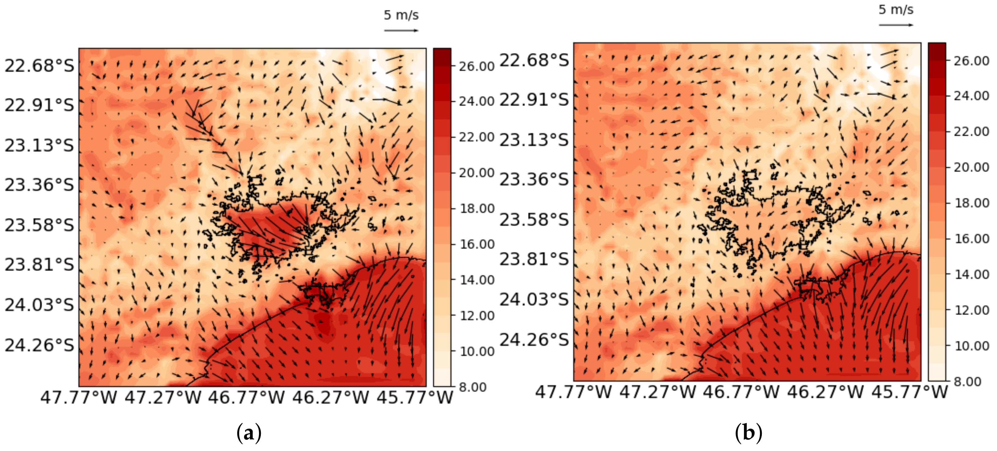
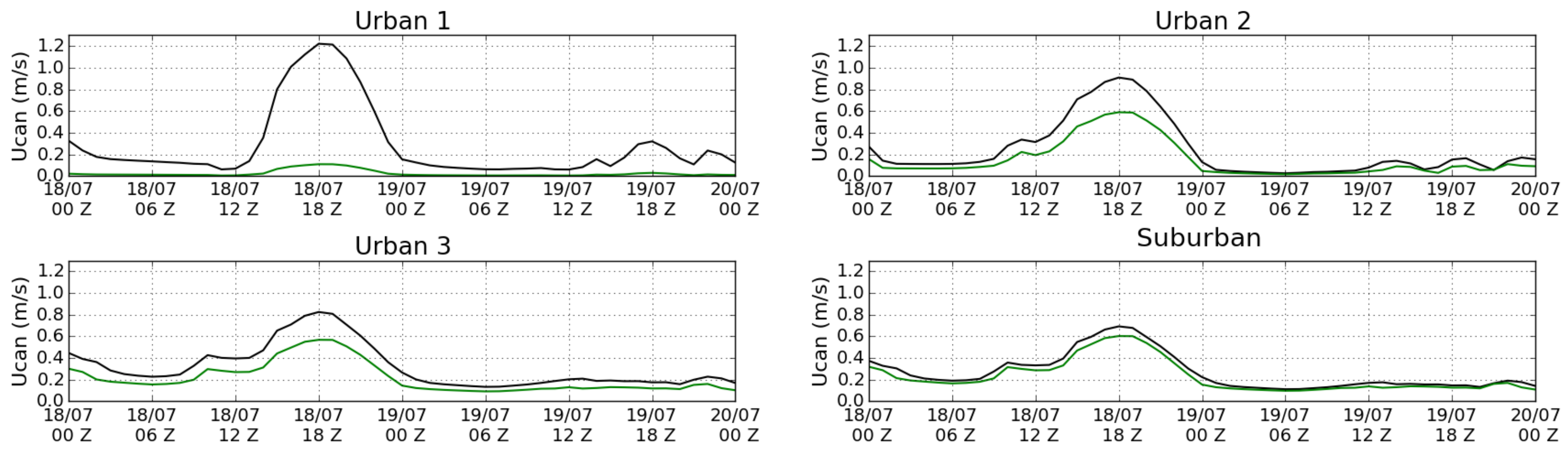
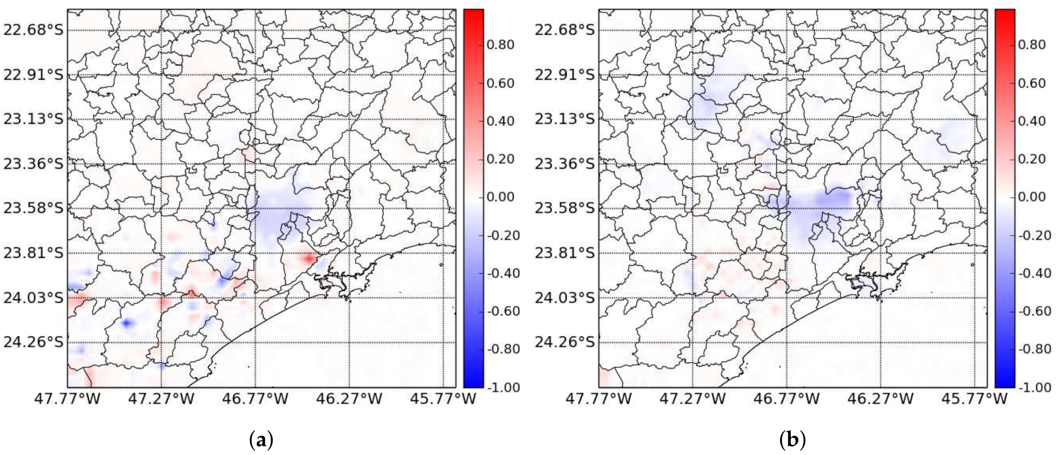
3.2. Sensitivity Tests

Sensitivity test analysis was based on Simulations A and C described in Section 2.3. In Simulation C, the aspect-ratios were computed from the observed SVFs for each urban type, as presented in Table 5.

These aspect-ratio values were inserted into the namelist of the BRAMS model, and the horizontal wind speed and the temperature inside canyon were compared with the original output of Simulation A. In Masson’s TEB formulations [4], the horizontal wind speed inside the urban canyon can be written as:

$$U_{can}=\frac{2}{\pi }exp\left(\frac{-1}{4}\frac{h}{w}\right)\frac{ln[(h/3)/z_{0town}]}{ln[(\Delta z+h/3)/z_{0town}]}\left|\overrightarrow{U_a}\right|$$

(5)

where $U_{can}$ is the wind intensity inside the urban canyon, $\Delta z$ is the height of first model level above the roof, $z_{0town}$ is the roughness length (approximately $h/10$) and $U_a$ is the wind intensity in the first level of the atmospheric model.

Figure 7 shows the daily evolution of horizontal wind speed inside the urban canyon for each urban type in MASP. In this figure, it can be noted that the horizontal wind intensity inside canyon for all urban types has higher intensities for Simulation C by reducing the values of aspect-ratio. The wind speed difference between Simulations A and C is up to 1.2 $\mathrm{m}{\mathrm{s}}^{-1}$ at 18Z on 18 July, for the urban type 1. In this urban type, the difference between the aspect-ratios is larger when compared with other urban land classes. This occurs because a higher aspect-ratio induces larger friction due to the presence of an extensive vertical surface (wall). In the case of Simulation A, the aspect-ratio is larger.

The air temperature inside the urban canyon is obtained from the energy budget and it is written as [4]:

$$T_{can}=\frac{\frac{T_s}{RE{S}_s}+\frac{2h}{w}\frac{T_w}{RE{S}_w}+\frac{T_a}{RE{S}_{top}}+\frac{H_{traffic}}{C_{pd}{\rho }_a(1-a_{bld})}}{\frac{1}{RE{S}_s}+\frac{2h}{w}\frac{1}{RE{S}_w}+\frac{1}{RE{S}_{top}}}$$

(6)

being $T_a$ the temperature (in Kelvin), RES the aerodynamic resistance (in $\mathrm{s}{\mathrm{m}}^{-1}$), $C_{pd}$ the specific heat at constant pressure of dry air (in $\mathrm{J}{\mathrm{kg}}^{-1}{\mathrm{K}}^{-1}$), ${\rho }_a$ the density of air ($\mathrm{kg}{\mathrm{m}}^{-3}$) at the first model level and $a_{bld}$ the urban built fraction area. The s, w and $top$ indexes stand for street, wall, and top of canyon level, respectively. The a index stands for the air temperature, corrected by the Exner function. Figure 8 shows the difference in the inside-canyon temperature field between Simulations A and C. At night, the temperature variation is mainly due to heat released from the surface in form of both sensible heat and radiation, while during the day the shortwave radiation retention implies the temperature increase of areas with tall buildings. In Figure 8a,c, it can be noted that the building height in Simulation C is important in long-wave emission due to the presence of larger wall surface area than Simulation C. The temperature difference in the canyon reaches up to 1.1 ${}^{\circ }$C 00Z on 19 July in the central region of MASP (area with larger buildings and larger aspect-ratio).

During the day (Figure 8b,d), the temperature difference inside the canyon reaches up to 0.19 ${}^{\circ }$C in suburban-like regions (less difference in aspect-ratio), and 0.96 ${}^{\circ }$C in the central region (greater difference in aspect-ratio). These differences are due to the type of urban canyon aspect-ratio that retains more solar radiation in the atmosphere. In the case of Simulation A, the reduction in aspect-ratio, while having same building height, requires a larger road width. The road has a smaller reflectance, absorbing more solar radiation. Therefore, the suburban region, which has higher buildings, has a smaller temperature difference between the two simulations.

4. Conclusions and Remarks

Observational SVF were used to improve the temperature and wind speed diagnostic of urban areas in the BRAMS mesoscale model. To do this, two kinds of simulations were performed: Simulation A, where the model was run using the original SVF equation, and Simulation B, where the mean observed SVF were used in each grid-point of the simulation domain. A digital camera equipped with a fish-eye lens was deployed to take photos of 37 street view points throughout the MASP. These SVF were included in the model as an input parameter, based on the averaged value for each urban type. Analyzing the statistical indexes $BIAS$, $RMSE$, and $D_{Pielke}$, and comparing with the observations, in general, the inclusion of the SVF showed an improvement in the simulations, especially in regions near areas with high density of buildings. As the SVF values increases, so does the fraction of visible sky. In this way, considering that the urban canyon becomes wider to keep aspect-ratio constant, more radiation reaches the street, which has a low albedo.

In addition, sensitivity tests were made with the model comparing the aspect-ratio value used in Simulation A and that obtained with observed values of SVF. The tests were done by evaluating the wind and temperature behavior in urban canyons. In this case, for each urban type, the wind intensity would be relatively large, since the width of the canyons would be larger. This happens due to the reduced friction on the walls of buildings. From a bulk point of view, it is equivalent to a smaller roughness length. Even without much difference in terms of the energy balance in the urban area, the temperature in the city center would be relatively lower due to the buildings shadowing effect. Therefore, the improvement of the treatment of the urban morphology in TEB with the inclusion of observed values of SVF was able to reproduce the expected effects in the thermal and dynamic field of the urban surface layer for the MASP. The representation of urban structure by means of observed SVF improves the wind field representation and temperature in the MASP.

By comparing the Simulations A and B, it can be seen that the use of observed SVF has improved the temperature evolution for Simulation B. In addition, Simulation C shows that the use of aspect-ratio based on the SVF data can provide unrealistic results in the wind and temperature inside the canyon. Thus, it is necessary to better define the dynamic aspects of the surface besides the use of the SVF for a better representation of urban morphology in these schemes. Thus, it follows that the importance of a good SVF database as an important tool in urban planning, targeting the thermal comfort of the city’s population. In addition, for a higher resolution simulation, it is recommended to improve this SVF database.

References

1. The World Bank. Urban Population (% of Total) the United Nations Population Division’s World Urbanization Prospects. Available online: https://data.worldbank.org/indicator/SP.URB.TOTL.IN.ZS (accessed on 18 December 2017).
2. Kusaka, H.; Kondo, H.; Kikegawa, Y.; Kimura, F. A simple single-layer urban canopy model for atmospheric models: Comparison with multi-layer and slab models. Bound.-Layer Meteorol. 2001, 101, 229–258. [Google Scholar] [CrossRef]
3. Martilli, A.; Clappier, A.; Rotach, M.W. An urban surface Exchange parameterization for mesoscale models. Bound.-Layer Meteorol. 2002, 104, 261–304. [Google Scholar] [CrossRef]
4. Masson, V. A physically-based scheme for the urban energy budget in atmospheric models. Bound.-Layer Meteorol. 2000, 94, 357–397. [Google Scholar] [CrossRef]
5. Hamdi, R.; Schayes, G. Sensitivity study of the urban heat island intensity to urban characteristics. Int. J. Climatol. 2007, 28, 973–982. [Google Scholar] [CrossRef]
6. Freitas, E.D.; Rozoff, C.; Cotton, W.R.; Silva Dias, P.L. Interactions of urban heat island and sea breeze circulations during winter over the Metropolitan Area of São Paulo—Brazil. Bound.-Layer Meteorol. 2007, 122, 43–65. [Google Scholar] [CrossRef]
7. Salamanca, F.; Martilli, A.; Tewari, M.; Chen, F. A Study of the Urban Boundary Layer Using Different Urban Parameterizations and High-Resolution Urban Canopy Parameters with WRF. J. Appl. Meteorol. Climatol. 2011, 50, 1107–1128. [Google Scholar] [CrossRef]
8. Giovannini, L.; Zardi, D.; de Franceschi, M.; Chen, F. Numerical simulations of boundary-layer processes and urban-induced alterations in an Alpine valley. Int. J. Climatol. 2014, 34, 1111–1131. [Google Scholar] [CrossRef]
9. Svensson, M.K. Sky view factor analysis—Implications for urban air temperature differences. Meteorol. Appl. 2004, 11, 201–211. [Google Scholar] [CrossRef]
10. Upmanis, H.; Chen, D. Influence of geographical factors and meteorological variables on nocturnal urban-park temperature differences A case study of summer 1995 in Goteborg, Sweden. Clim. Res. 1999, 13, 125–139. [Google Scholar] [CrossRef]
11. Oke, T.R. Boundary Layer Climates, 2nd ed.; Routledge: London, UK, 1987; p. 435. [Google Scholar]
12. Watson, I.; Johnson, G. Graphical Estimation of sky-view factor in urban environments. J. Climatol. 1987, 7, 193–197. [Google Scholar] [CrossRef]
13. Santamouris, M. Energy and Climate in the Urban Built Environment; James & James Science Publishers Ltd.: London, UK, 2001. [Google Scholar]
14. Eliasson, I. Urban Nocturnal Temperatures, street geometry and land use. Atmos. Environ. 1996, 30, 379–392. [Google Scholar] [CrossRef]
15. Marciotto, E.R.; Oliveira, A.P.; Hanna, S.R. Modeling study of the aspect ratio influence on urban canopy energy fluxes with a modified wall-canyon energy budget scheme. Build. Environ. 2010, 45, 2497–2505. [Google Scholar] [CrossRef]
16. Hanna, S.; Marciotto, E.R.; Britter, R. Urban Energy Fluxes in Built-Up Downtown Areas and Variations across the Urban Area, for Use in Dispersion Models. J. Appl. Meteorol. Climatol. 2011, 50, 1341–1353. [Google Scholar] [CrossRef]
17. Marciotto, E.R. Variability of energy fluxes in relation to the net-radiation of urban and suburban areas: A case study. Meteorol. Atmos. Phys. 2013, 121, 17–28. [Google Scholar] [CrossRef]
18. Georgakis, C.; Santamouris, M. Experimental investigation of air flow and temperature distribution in deep urban canyons for natural ventilation purposes. Energy Build. 2006, 38, 367–376. [Google Scholar] [CrossRef]
19. Marciotto, E.R.; Fisch, G. Wind tunnel study of turbulent flow past an urban canyon model. Environ. Fluid Mech. 2013, 13, 403–416. [Google Scholar] [CrossRef]
20. Giovannini, L.; Zardi, D.; de Franceschi, M. Characterization of the Thermal Structure inside an Urban Canyon: Field Measurements and Validation of a Simple Model. J. Appl. Meteorol. Climatol. 2013, 52, 64–81. [Google Scholar] [CrossRef]
21. Ali-Toudert, F.; Mayer, H. Numerical study on the effects of aspect ratio and orientation of an urban street canyon on outdoor thermal comfort in hot and dry climate. Build. Environ. 2006, 41, 94–108. [Google Scholar] [CrossRef]
22. Memon, R.A.; Leung, D.Y.C.; Liu, C.H. Effects of building aspect ratio and wind speed on air temperatures in urban-like street canyons. Build. Environ. 2010, 45, 176–188. [Google Scholar] [CrossRef]
23. Chen, L.; Ng, E.; An, X.; Ren, C.; Lee, M.; Wang, U.; He, Z. Sky view factor analysis of street canyons and its implications for daytime intra-urban air temperature differentials in high-rise, high-density urban areas of Hong Kong: A GIS-based simulation approach. Int. J. Climatol. 2012, 32, 121–136. [Google Scholar] [CrossRef]
24. Sparrow, E.M.; Cess, R.D. Radiation Heat Transfer; Brooks/Cole Publishing Company: Belmont, CA, USA, 1978. [Google Scholar]
25. Grimmond, C.S.B.; Potter, S.K.; Zutter, H.N.; Souch, C. Rapid Methods to estimate Sky-View Factors applied to Urban Areas. Int. J. Climatol. 2001, 21, 903–913. [Google Scholar] [CrossRef]
26. Hammerle, M.; Gál, T.; Unger, J.; Matzarakis, A. Introducing a script for calculating the sky view factor used for urban climate investigations. Acta Climatol. Chorol. 2011, 45, 83–92. [Google Scholar]
27. Hammerle, M.; Gál, T.; Unger, J.; Matzarakis, A. Comparison of models calculating the sky view factor used for urban climate investigations. Theor. Appl. Climatol. 2011, 105, 521–527. [Google Scholar] [CrossRef]
28. Ibrahim, A.A.; Nduka, I.C.; Iguisi, E.O.; Ati, O.F. An Assessment of the impact of Sky View Factor (SVF) on the Micro-climate of Urban Kano. Aust. J. Basic Appl. Sci. 2011, 5, 81–85. [Google Scholar]
29. Santos, I.G.; Lima, H.G.; Assis, E.S. A graphical method for the Sky View Factor calculation in the Urban Heat Island Studies. In Proceedings of the 20th Passive and Low Energy Architeture, Santiago, Chile, 9–12 November 2003. [Google Scholar]
30. Andrade, M.F.; Ynoue, R.; Freitas, E.D.; Todesco, E.; Vela, A.G.; Ibarra, S.; Martins, L.D.; Martins, J.A.; Carvalho, V.S.B. Air Quality forecasting system of Southeastern Brazil. Front. Environ. Sci. 2015, 3, 9. [Google Scholar] [CrossRef]
31. Gouvêa, M.L. Cenários de Impacto das Propriedades da Superfície Sobre o Conforto térmico Humano na Cidade de São Paulo. Master’s Thesis, University of São Paulo, São Paulo, Brazil, 2007. [Google Scholar]
32. Stewart, I.D.; Oke, T.R. Local Climate Zones for Urban Temperature Studies. Bull. Am. Meteorol. Soc. 2012, 93, 1879–1900. [Google Scholar] [CrossRef]
33. Morais, M.V.B.; Freitas, E.D.; Urbina Guerrero, V.V.; Martins, L.D. A modeling analysis of urban canopy parameterization representing the vegetation effects in the Megacity of São Paulo. Urban Clim. 2016, 17, 102–115. [Google Scholar] [CrossRef]
34. Morais, M.V.B.; Marciotto, E.R.; Urbina Guerrero, V.V.; Freitas, E.D. Effective albedo estimates for the Metropolitan Area of São Paulo using empirical sky-view factors. Urban Clim. 2017, 21, 183–194. [Google Scholar] [CrossRef]
35. Freitas, S.R.; Longo, K.M.; Silva Dias, M.A.F.; Chatfield, R.; Silva Dias, P.; Artaxo, P.; Andreae, M.O.; Grell, G.; Rodrigues, L.F.; Fazenda, A.; et al. The Coupled Aerosol and Tracer Transport Model to the Brazilian developments on the Regional Atmospheric Modeling System (CATT-BRAMS)—Part 1: Model description and evaluation. Atmos. Chem. Phys. 2009, 9, 2843–2861. [Google Scholar] [CrossRef]
36. Freitas, S.R.; Panetta, J.; Longo, K.M.; Rodrigues, L.F.; Moreira, D.S.; Rosário, N.E.; Silva Dias, P.L.; Silva Dias, M.A.F.; Souza, E.P.; Freitas, E.D.; et al. The Brazilian developments on the Regional Atmospheric Modeling System (BRAMS 5.2): An integrated environmental model tuned for tropical areas. Geosci. Model Dev. 2017, 10, 189–222. [Google Scholar] [CrossRef]
37. Lee, T.J. The Impact of Vegetation on the Atmospheric Boundary Layer and Convective Storms. Ph.D. Thesis, Colorado State University, Fort Collins, CO, USA, 1992. [Google Scholar]
38. Walko, R.L.; Band, L.E.; Baron, J.; Kittel, T.G.F.; Lammers, R.; Lee, T.J.; Ojima, D.; Pielke, R.A.; Taylor, C.; Tague, C.; et al. Coupled atmosphere-biophysics-hydrology models for environmental modeling. J. Appl. Meteorol. 2000, 39, 931–944. [Google Scholar] [CrossRef]
39. SVMA (Secretaria do Verde e Meio Ambiente). Atlas ambiental de São Paulo. Available online: http://atlasambiental.prefeitura.sp.gov.br/conteudo/coberturavegetal/vegapres02.pdf (accessed on 13 November 2017).
40. Klemp, J.B.; Wilhelmson, R.B. The simulation of three-dimensional convective storm dynamics. J. Atmos. Sci. 1978, 35, 1070–1096. [Google Scholar] [CrossRef]
41. Chen, C.; Cotton, W.R. The physics of the marine stratocumulus-capped mixed layer. Bound.-Layer Meteorol. 1987, 25, 289–321. [Google Scholar] [CrossRef]
42. Smagorinsky, J. General circulation experiments with the primitive equations: 1. The basic experiment. Mon. Weather Rev. 1963, 91, 99–164. [Google Scholar] [CrossRef]
43. Hill, G.E. Factors controlling the size and spacing of cumulus clouds as revealed by numerical experiments. J. Atmos. Sci. 1974, 31, 646–673. [Google Scholar] [CrossRef]
44. Lilly, D.K. On the numerical simulation of buoyant convection. Tellus 1962, 2, 148–172. [Google Scholar] [CrossRef]
45. Wilks, D.S. Statistical Methods in the Atmospheric Sciences, 2nd ed.; Academic Press: San Diego, CA, USA, 2006. [Google Scholar]
46. Hallak, R.; Pereira Filho, A.J. Metodologia para análise de desempenho de simulaćões de sistemas convectivos na região metropolitana de São Paulo com o modelo ARPS: Sensibilidade a variaćões com os esquemas de advecćão e assimilaćão de dados. Rev. Bras. Meteorol. 2011, 26, 591–608. [Google Scholar] [CrossRef]
47. Pielke, R.A., Sr. Mesoscale Meteorological Modeling, 3rd ed.; Academic Press: San Diego, CA, USA, 2002. [Google Scholar]
48. Daley, R. Atmospheric Data Analysis, 1st ed.; Cambridge Press: New York, NY, USA, 1991; p. 457. [Google Scholar]
Figure 1. Result of the surface classification used to obtain the SVF values, with a grid spacing of 500 m for the MASP. The blue color corresponds to a suburban type, cyan color to the urban type 3, yellow color to the urban type 2 and red color to the urban type 1.
Sustainability 10 02183 g001
Figure 2. Places where the observational values of SVF were obtained (blue dots). The bottom figure amplifies the red area where the points were selected in MASP.
Sustainability 10 02183 g002
Figure 3. Nesting grids and NDVI data (inside 2nd domain) used in the simulations.
Sustainability 10 02183 g003
Figure 4. Examples of fish-eye lens photos: (a) a downtown neighborhood (Site 1) classified as urban 1, with tall buildings and high aspect-ratio; and (b) a suburban neighborhood (Site 37) classified as urban 3, with low aspect-ratio.
Sustainability 10 02183 g004
Figure 5. Daily evolution of air temperature in degrees Celsius at 2 m agl: (a) São Caetano; (b) Guarulhos; (c) Congonhas; (d) Mirante de Santana; and (e) IAG. The continuous gray line represents Simulation A, the black dashed line represents Simulation B, and solid black line is the observed temperature. Local Standard Time = UTC − 3 h.
Sustainability 10 02183 g005
Figure 6. Temperature at 2 m ( C) and wind field (m/s) for July 19th at 00Z for: (a) Simulation A; and (b) Simulation B.
Sustainability 10 02183 g006
Figure 7. Daily evolution of horizontal wind speed inside the urban canyon for a point in each urban type in MASP. Green line, Simulation A, and black line, Simulation C. Local Standard Time = UTC − 3 h.
Sustainability 10 02183 g007
Figure 8. Temperature difference field inside the canyon for Simulation A with aspect-ratio presented in Table 5 and for Simulation C for: (a) 00Z and (b) 12Z on 18 July; and (c) 00Z and (d) 12Z on 19 July. Local Standard Time = UTC − 3 h.
Sustainability 10 02183 g008aSustainability 10 02183 g008b