Spatial Variation of Urban Thermal Environment and Its Relation to Green Space Patterns: Implication to Sustainable Landscape Planning


1
XJTLU-Suzhou Urban & Environment Research Institute, Suzhou 215200, Jiangsu, China
2
XJTLU-Huai’an Research Institute of New-type Urbanization, Huai’an 223005, Jiangsu, China
3
Department of Environmental Science, Xi’an Jiaotong-liverpool Uiversity (XJTLU), Suzhou 215123, Jiangsu, China
*
Author to whom correspondence should be addressed.
Sustainability 2018, 10(7), 2249; https://0-doi-org.brum.beds.ac.uk/10.3390/su10072249
Submission received: 28 May 2018
/
Revised: 15 June 2018
/
Accepted: 26 June 2018
/
Published: 29 June 2018
(This article belongs to the Special Issue Urban Remote Sensing: Sustainability of Earth’s Environment, Resources and Ecology)
Abstract
:The rapid changes of land covers in urban areas are one of major environmental concerns because of their environmental impacts. Such land cover changes include the transformation of green space to impervious surface, and the increase of land surface temperature (LST). The objective of this study was to examine the spatial variation of urban landscape composition and configuration, as well as their influences on LST in Suzhou City, China. Landsat-8 image was processed to extract land covers and retrieve LSTs that were used to study relationship between spatial variation of LST and land covers. The results indicated that there was a significantly negative correlation between mean LST and green space coverage along the urban–rural gradients. With every 10% increased green space coverage, the mean LST drop was about 1.41 °C. A grid-base analysis performed at various grid sizes indicated that an increase in the percentage of surface water body area has a greater cooling effect of the mean LST than a vegetation increase. The mean LST had a significantly negative correlation with both the shape and aggregation indexes of the green space patches. Our results suggest that the sustainable landscape planning of green space in a typical city with a large water area should include both the vegetation and the surface water covers. The increased percentage of vegetation and surface water covers had the greatest cooling effect on an urban thermal environment, which is one of the ecosystem services that green space provides. A dense distribution of green space patches with complex shapes should be considered in urban sustainable landscape planning for increasing ecosystem services.
1. Introduction
In recent years, with the rapid development of society and the economy, the function of urban green space has been expanded from the urban landscape and cultural recreation to ecosystem services. As an important part of urban green infrastructures, the function of urban green space is also related to the quality of the local environment and the health of the residents [1,2], and plays an important role in urban ecosystems, which can reduce greenhouse gas, regulate the urban microclimate [3], reduce energy consumption [4,5], and maintain ecological security [6,7], which are among a wide range of ecosystem services [8]. The cooling effect of urban green space is regarded as an ecosystem regulating service [9,10]. However, rapid urbanization leads to a significant transformation of green space to impervious surface, urbanization profoundly influences biodiversity and ecosystem function; one of the ecological consequences of urbanization is the urban heat island (UHI) effect [11]. This phenomenon is particularly serious in the rapidly growing cities in China [12,13,14,15,16]. Urban forms, such as land covers, building density, and building height, often have a stronger influence on LST [17,18,19]. Green space, water bodies, green roofs, and vertical greenery have been identified as an effective strategy to moderate the negative effects of UHI through shading, evaporative cooling, and modifying airflows and heat exchange [20,21,22,23]. Reducing the adverse environmental effects of UHI is consistent with the United Nations’ Sustainable Development Goal 11: Sustainable Cities and Communities. Understanding the spatial variation of urban thermal environment and its relation to green infrastructure is therefore of great significance to adjust spatial patterns of urban green space and reduce the UHI in sustainable urban planning.
Urban thermal environment can be quantified in two ways. Traditionally, it’s mainly derived from the meteorological observational data, and this data source is a good indication of the monitoring points and their surroundings [16,24]. However, because of research scaling issues of observational data, it’s difficult to accurately reflect the spatial variation [25]. The application of thermal infrared remote sensing technology can effectively overcome the spatial restrictions of observational data, and it makes it possible to provide visual spatial patterns of LST, although it only provides an instantaneous measurement of temperature during the day. Currently, the research on remotely sensed LST is mainly focused on its spatial-temporal characteristics [26,27], change process, and its influence factors [28]. Many researchers focus their work on using remote sensing data for examining some correlations among LST, vegetation indexes [13,29,30,31], landscape composition, and configuration.
A previous study indicated the composition and spatial pattern of paved surfaces have drastic impacts on LST [32]. The increased percentage of green space was an important predictor of LST, and the composition of land cover features is more important in determining LST than their configuration [33,34]. Besides, landscape configuration should never be ignored [35], it is noteworthy that the relationship between LST and abundance of green space was consistently negative at different satellite image resolutions, but the relationship between LST and spatial configuration of green space varied by spatial resolution [36]. Thus, considering the influence of image resolution, we take Landsat images as examples to review the following literatures. Some researchers found that urban green space configurations with aggregated patterns and patch sizes have the strongest cooling effect on UHI [37,38]. However, Shih et al. [39] revealed that green space size, shape, and greenness may have limited effect for mitigating UHI at the area nearby green space. The edge characteristics are also important spatial features that could help explain the variability of LST [33]. Maimaitiyiming et al. [40] indicated that configuration of green space as expressed by the joint effect of patch density and edge density was the most deterministic metric that affects LST. These analyses showed regional differences in the factor of green space affecting LST.
In general, the effect of urban green space on reducing UHI should be fixed and does not change with the grid sizes. However, the relationship between LST and landscape composition still has some uncertainties with different grid sizes. Xiao et al. [41] found that the correlation between impervious surface density and mean LST increased as the grid size increased from 30 m to 960 m in Beijing. Myint et al. [42] indicated that there were some differences in correlation between temperature and vegetation with the use of different window sizes. Kong et al. [43] found a significantly negative correlation exists between the percentage of forest-vegetation and LST with the increase of window sizes. Estoque et al. [44] revealed the influence of green space on the variability of LST in smaller grid size in the megacities of Southeast Asia.
Considering the above cases, there are two main problems in green space–LST relationship research: (1) the factor of green space configuration shows regional differences in cooling effect; (2) there are some uncertainties about the effect of landscape composition on LST when using different grid sizes. Indeed, a number of studies examined the relationship between LST and the landscape composition and configuration. However, such a study in a typical city with a large area of water bodies is still lacking. The objective of this study was to examine the spatial variation of urban landscape composition and configuration, and to assess their influences on LST in Suzhou City, China. Utilizing the Landsat-8 image as the data source, this study answered research questions relating following facets: (1) test whether the above-mentioned characteristics are fit in a water city Suzhou; (2) verify the effect of landscape composition on LST with the increase of grid size; (3) investigate spatial variation of urban landscape composition and configuration, as well as their effects on LST in Suzhou City.
2. Materials and Methods
2.1. Study Area
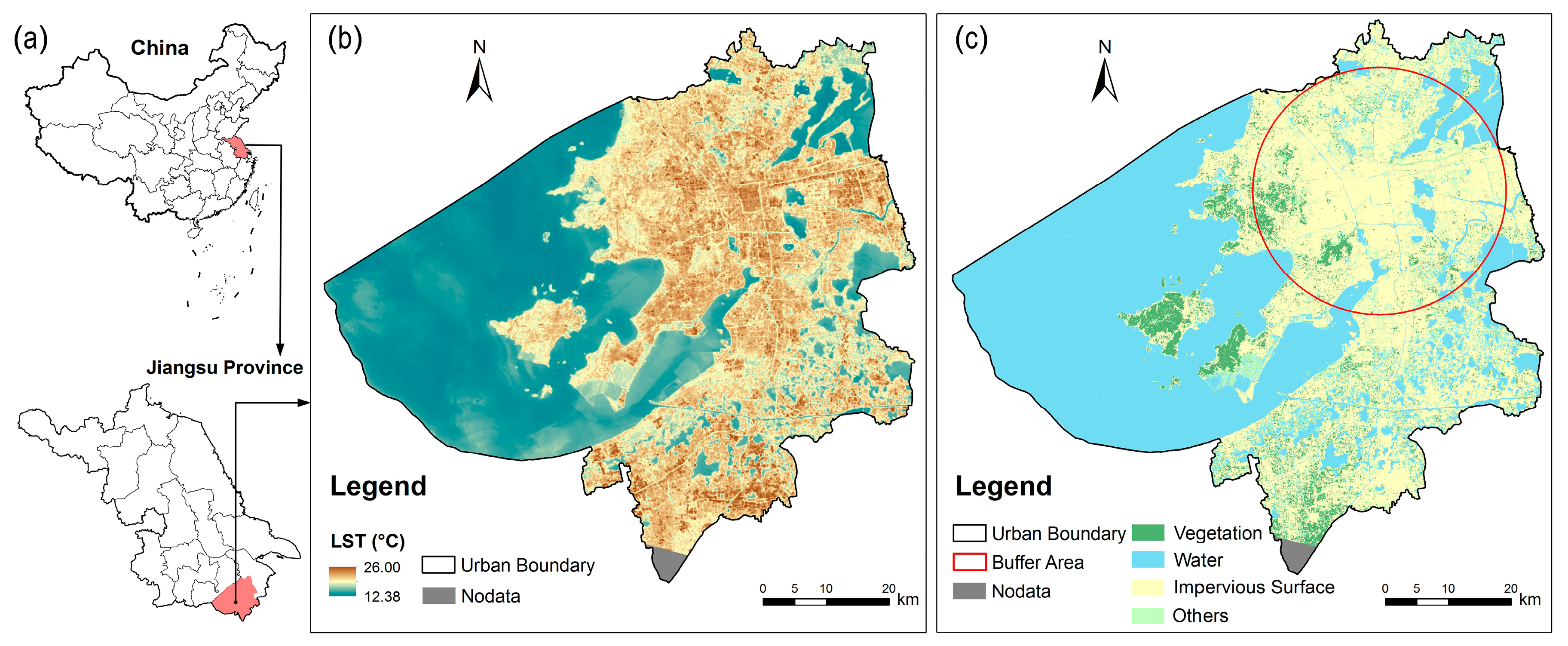
Suzhou is located in South-Eastern Jiangsu Province in the center of the Yangtze Delta in China (119°55′–121°20′ E, 30°47′–32°02′ N), about 100 km northwest of Shanghai. It covers a total area of 4652.84 km2 and the urban built-up area is 458.29 km2. Suzhou is a prefecture-level city with a resident population of 5.51 million in its built-up area, and a total resident population of 10.64 million in its administrative area in 2016. In the last three decades, Suzhou experienced profound economic development and rapid urbanization, and with significant UHI effect after 2000. Previous results found that UHI was highly correlated with the spatial pattern of urban construction in Suzhou [45]. The UHI has taken the old town as the center and extended to the surrounding areas (6 km away from the center of the city), especially in the east and south of the Suzhou [46].
2.2. Data
One cloud-free Landsat-8 operational land imager (OLI) and thermal infrared sensor (TIRS) image, which covered the study area (Row/Path: 038/119), were collected on 5 March 2016 from United States Geological Survey (USGS) Earth Resources Observation and Science (EROS) Center. Thermal infrared band (B10) in Landsat-8 OLI/TIRS was used for LST retrieval. Spectral index-based methods were used to classify the image of study areas into four land cover types (i.e., vegetation, water, impervious surface, and others).
2.3. Materials and Methods
2.3.1. LST Retrieval
Landsat-8 thermal infrared band data were utilized to map LST. First, we converted calibrated digital numbers to absolute units of at-sensor spectral radiance. Second, at-sensor spectral radiance was converted to at-sensor brightness temperature. After calculating the brightness temperature values, the LST was converted as follows [3,47]:
where T is the effective at-satellite temperature in Kelvin; K2 is the calibration constant 2 (1321.08); K1 is the calibration constant 1 (774.89); and LT is the radiance of a blackbody target of kinetic temperature in W·m−2·sr−1·μm−1.
where Lλ is the at-sensor radiance in W·m−2·sr−1·μm−1; ε is the land surface emissivity; L↑ and L↓ are the upwelling and downwelling atmospheric radiance in W·m−2·sr−1·μm−1, respectively; and τ is the total atmospheric transmissivity between the land surface and the sensor. The last three parameters can be estimated by NASA’s website (http://atmcorr.gsfc.nasa.gov/).
2.3.2. Land Covers
Normalized difference vegetation index (NDVI), modified normalized difference water index (MNDWI), and normalized difference impervious surface index (NDISI) were calculated by Landsat-8 OLI/TIRS multispectral image, and a manually determined threshold was applied in order to extract the vegetation, water body, and impervious surface. Based on 200 randomly selected points generated by ArcGIS (Version 10.2, Environmental Systems Research Institute, Redlands, United States of America), the classification accuracies were checked using the Google Earth image.
2.3.3. Urban–Rural Gradient Analysis and Grid-Based Analysis
In order to identify the spatial variation of LST and land covers along an axis going from city center to the rural area, multiple ring buffer zones have been created around city center. Fan et al. [48] suggested that a reasonable size for examining the vegetation–LST relationship is 200 m by ASTER images. Considering the scaling effect of satellite sensors, we set the buffer with a distance interval of 300 m in this paper. This is consistent with previous research [36,44]. An intersection point of Renmin road and Ganjiang road has been defined as the center of multiple ring buffer zones. Different sizes of polygon grids were created to clip land covers and LST. In this particular analysis, the grids that contained only water (accounted for 100% of the total area) were not included. In each buffer zone and grid size, the mean LST and the percentage of land covers were calculated.
2.3.4. Landscape Metrics
As landscape metrics have been widely used to measure landscape pattern, green space and impervious surface with 30 m spatial resolution were used as landscape unit for analysis in this study. The mean community area was 10.15 km2 in Suzhou City, and its mean service radius was 1 km to 1.5 km (according to the Chinese National Standard GB 50180—Code of Urban Residential Areas Planning & Design). Thus, we divided the study area into polygon grids of 3-km size. Besides, this method was also consistent with Estoque et al. [44]. Those grids that water bodies accounted for 100% of the total area were not selected as samples for analysis. A total of 50 representative selected samples were used to clip land covers and LST. For each sample, four class-level landscape metrics were introduced to be calculated by Fragstats4.2 (a computer software program designed to compute a wide variety of landscape metrics for categorical map patterns. Sources: http://www.umass.edu/landeco/research/fragstats/fragstats.html). The patch neighbour was defined by the “8-cell rule”. These four indices are expressed in equations as follows.
where MPS is the mean plaque size in hectare; ai is the area of the patch in hectare; and n is the number of the patches.
where SI is the shape index; Pi is the perimeter of patch in metre; and ai is the area of the patch in hectare. This shape index measures the complexity of patch shape compared with a standard shape (square) of the same size, and SI equals 1 when the patch is square and increases without limit as patch shape becomes more irregular.
where AI is the aggregation index; and g and maxg are the number and maximum number of like adjacencies between pixels of patch based on the single-count method, respectively. AI equals 0 when the patch type is maximally disaggregated, AI increases as the patch type is increasingly aggregated and equals 100 when the patch type is maximally aggregated into a single, compact patch.
where FD is the fragmentation index; n is number of patches; and Ai is the total area of the patch in hectare. FD increases as the patch type is increasingly fragmented.
2.3.5. Statistical Analysis
Pearson correlation analysis, scatter plots, and linear fitting were used to determine the relationships between mean LST and the percentage of impervious surface and green space. The relationship between mean LST and landscape metrics was examined using Pearson correlation analysis.
3. Results
Figure 1 shows the distribution of LST and land covers (the threshold values of NDVI, MNDWI, and NDISI were 0.42, 0 and 0.10, respectively) in 2016. The confusion matrix showed that the overall classification accuracy was 84.0%, and the classification accuracy of vegetation, water, and impervious surface were 79.5%, 82.9%, and 89.9%, respectively.
3.1. Urban–Rural Gradient Analysis
Vegetation and water body had a significant influence on LST distribution in Suzhou. This result demonstrates that the highest mean LST was found in the impervious surface (24.10 °C), followed by vegetation (23.05 °C), and the lowest mean LST was given by water body (15.16 °C). This pattern suggests that vegetation and water body play an important role in alleviating the UHI effect. Some studies indicate that water bodies have a cooling effect and can lower the temperature of their surroundings [43,49,50,51,52]. This result in Suzhou confirms the association between cool areas with relatively low LST and large open water bodies, such as rivers, lakes, and ponds. A previous study suggested that a combination of NDVI and MNDWI would be the best indicator of LST [53]. Consequently, the vegetation and surface water covers were combined as green space for the following analysis.
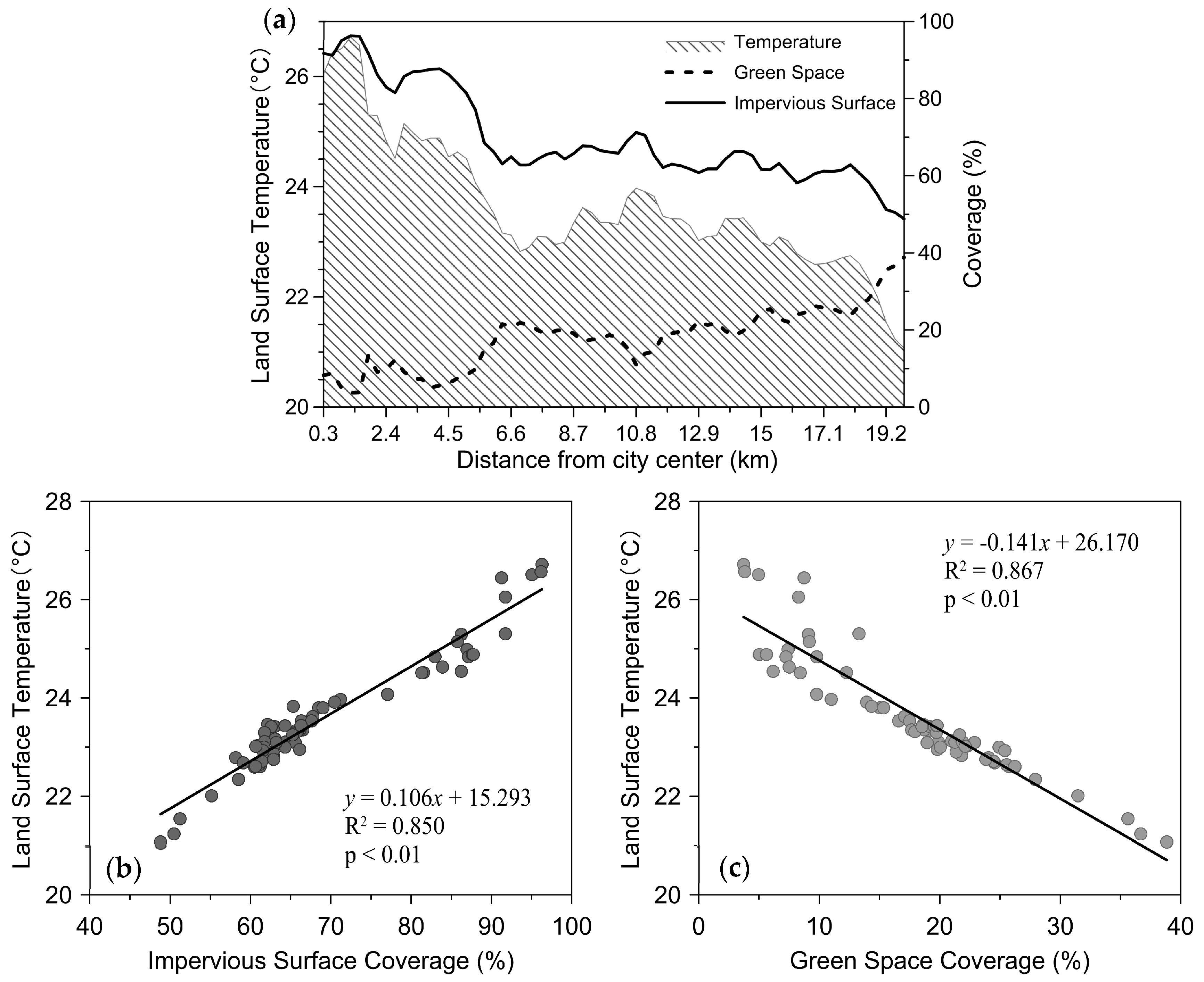
Along an axis going from the city center to the rural area (Figure 2a), impervious surface coverage and mean LST had a similar spatial pattern; both were gradually decreasing in rural area, contrasting the spatial pattern of green space coverage. Specifically, the highest mean LST does not appear in the center of the city, and the mean LST reached its peak at about 1.5 km distance from the city center. Considering that some area of the parks is located in this area, it may help explain why the zones close to the city center did not have the highest mean LST. The results also show that the mean LST of the city center was about 25.10 °C from zone 0 km to zone 6 km, which was higher than that of outer areas (23.00 °C). Because of the cooling effect of the Jinji Lake, Dushu Lake, and Yangcheng Lake, which lie to the east of the Suzhou City, the mean LST dropped significantly from zone 6 km to zone 9 km (mean LST declined 1.95 °C, and surface water coverage increased 9.43%). The mean LST has reached a third highest peak at zone 10.8 km from the city center, after which it decreased along the gradient direction.
After calculating the mean LST, green space coverage, and impervious surface coverage in each buffer zone, the scatter plots between impervious surface (green space) coverage and mean LST are drawn at the same time. A significant correlation between mean LST and the percentage of impervious surface (positive) and green space (negative) along an axis going from city center to the rural area (Figure 2b,c) can be found. From the results of linear fitting, it appears that regression equations passed significant inspection of Student’s t-test. With every 10% increase in impervious surface coverage, the mean LST was raised by about 1.06 °C. By contrary, with every 10% increase in green space coverage, the mean LST drop was about 1.41 °C.
3.2. Grid-Based Analysis
Table 1 shows the characteristics of mean LST and its relation to land covers, and the correlation coefficients between the percentage of impervious surface and green space (including water and vegetation) and mean LST passed the significance test (p < 0.01). With the increase of grid size, the impervious surface coverage and mean LST decreased from 72.51% and 23.34 °C to 64.14% and 22.44 °C, respectively. Further, the percentage of green space and water body increased from 21.95% and 10.73% to 30.21% and 20.21%, respectively. However, there was little change in vegetation coverage, its value was stable at 10.38 ± 0.53%. This analysis performed at various grid sizes indicated that there was no significant effect of the urban vegetation on reducing the LST with the use of different grid sizes. Furthermore, an increase in the percentage of surface water body area had a greater cooling effect on the mean LST than a vegetation increase.
3.3. Landscape Patterns
Based on the above methods, a total of 50 representative selected polygon samples of 3-km size have been used as study samples on the community scale. We calculated the plaque size, shape index, aggregation index, and fragmentation index of impervious surface and green space in these samples. By analysing their relation with mean LST and landscape metrics, we can quantitate the effect of landscape spatial patterns on mean LST. The results are shown in Table 2.
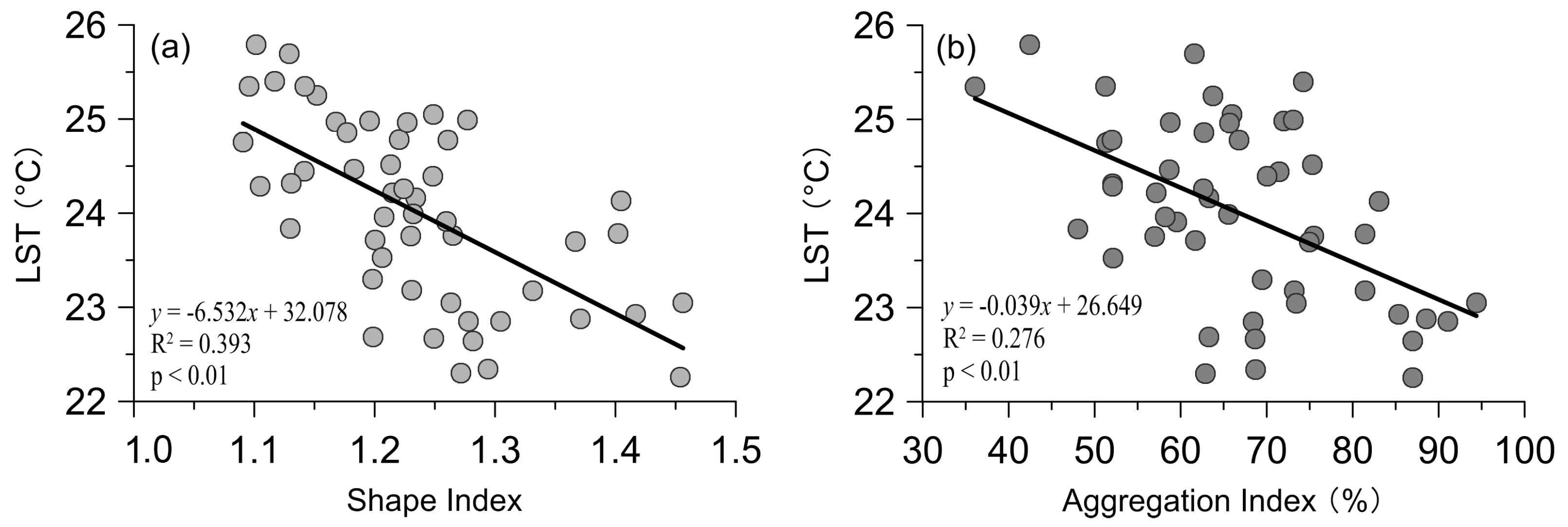
Specifically, the mean LST had a significantly negative correlation with both the shape and aggregation indexes of the green space patches, but it had a significantly positive correlation with the fragmentation index. On the contrary, the correlation of mean LST and landscape metrics of impervious surface was contrary to the above results. However, the correlation between the shape index of impervious surface and the mean LST has not passed the significance test, as well as the fragmentation index.
As a measure of the degree of spatial aggregation of landscape components, the aggregation index showed a significant correlation with mean LST. Figure 3 shows the scatter plots between the mean LST and aggregation index, the shape index of the green space patches. It indicated that the more concentrated and complex the spatial distribution of the green space, the lower the mean LST. On the contrary, the relation between concentrated distribution of impervious surface and mean LST was contrary to the above results. Thus, it can be indicated that the more urban green space is concentrated with complex shapes in spatial distribution, the more obvious the cooling effect on land surface.
4. Discussion
This study first analyzed the spatial variation of LST in Suzhou City, and a typical UHI profile was displayed by multiple ring buffer zones. Our results demonstrated that the highest mean LST was found in the impervious surface (24.10 °C), followed by vegetation (23.05 °C), and the lowest mean LST was given by water body (15.16 °C). There was a significantly negative correlation between mean LST and the percentage of green space along an axis going from city center to the rural area. With every 10% increased green space coverage, the mean LST drop was about 1.41 °C. The impervious surface coverage and mean LST were gradually decreasing in the rural area, contrasting the spatial pattern of green space coverage; this result is consistent with Xu et al. [45]. The results of the urban–rural gradient analysis indicated that the mean LST of city center was about 25.10 °C from zone 0 km to zone 6 km, which is higher than that of outer areas (23.00 °C). Because of the cooling effect of three large water bodies that lie to the east of the Suzhou City, the mean LST has declined 1.95 °C from zone 6 km to zone 9 km from the city center. The two national industrial parks on both sides of the urban area are important driving force behind the rapid urbanization, and the mean LST has reached a third highest peak in this area. This result indicated that location of high temperature zones also correspond with the overall pattern of urban development in recent years.
This study focused on examining the effects of landscape composition on LST with the increase of grid size in Suzhou City. From the results of the grid-based analysis, the larger the size of grid, the higher the green space coverage (including water and vegetation), and the lower the mean LST. However, vegetation coverage was stable at 10.38 ± 0.53% with the increase of grid size, and water coverage increased from 10.73% to 20.21%. The correlation analysis performed at various grid sizes indicated that there was no significant effect of the urban vegetation on reducing the LST with the use of different grid sizes. Furthermore, an increase in the percentage of surface water body area had a greater cooling effect of the mean LST than a vegetation increase. This is consistent with the previous studies, which demonstrated that water bodies have a great effect on the correlation between the urban form factors and the LST [49,52]. Previous studies have also shown the water bodies with a large area have a better cooling effect on the urban thermal environment [51,52]. Kong et al. [43] found that a significant relationship exists between the percentage of forest vegetation and LST with the increase of window sizes. This is because, in their study, a higher percentage (47.5%) of forest-vegetation could create a greater cooling effect. In our case, however, urban vegetation coverage was stable at 10.38 ± 0.53%. If one added water bodies to the green space, we found a significant relationship exists between the percentage of green space and LST with the increase of window sizes. Suzhou is a typical city with a large area of water bodies. With the increase of grid size, the percentage of surface water body area increases, and the mean LST decreases. An increase in the percentage of surface water body area had a greater cooling effect on the mean LST than a vegetation increase, and the regulation of the spatial pattern of urban green space in a typical city with a large water area should include both the vegetation and the surface water covers.
In addition, this study analyzed the spatial pattern of green space and its relation with LST. In terms of landscape pattern on the community scale, the mean LST had a significantly negative correlation with both the shape and the aggregation indexes of the green space patches. Similar results were also found in Zhou et al. [33] and Li et al. [34]. The scatter plots between aggregation index, shape index, and LST indicated that the more urban green space is concentrated with complex shapes in spatial distribution, the more obvious the cooling effect on land surface.
5. Conclusions
The Landsat-8 OLI/TIRS image and spectral index-based methods were used to retrieve LST and extract land covers. Urban–rural gradient, grid-based methods, and landscape metrics were adopted to analyze the spatial patterns of the LST and the land covers. A typical UHI profile was showed by multiple ring buffer zones in Suzhou City. Our results indicated that there was a significantly negative correlation between the mean LST and the green space coverage along an axis going from the city center to the rural area. A grid-based analysis performed at various grid sizes indicated that an increase in the percentage of surface water body area has a greater cooling effect of the mean LST than a vegetation increase. Besides, this study shows that the mean LST had a significantly negative correlation with both the shape and aggregation indexes of the green space patches.
In conclusion, the sustainable landscape planning of green space in a typical city with a large water area should include both the vegetation and the surface water covers. The increased percentage of vegetation and surface water covers had the greatest cooling effect on an urban thermal environment, which is one of ecosystem services that green space provides. A dense distribution of green space patches with complex shapes should be considered in urban sustainable landscape planning for increasing ecosystem services.
Author Contributions
All authors contributed equally to this work. All authors have read and approved the final manuscript.
Funding
This research was funded by the Scientific Research Projects of Huai’an City (HAN2015022).
Acknowledgments
The authors would like to thank Xue Chen and Noel Juvigny-Khenafou for their technical support.
Conflicts of Interest
The authors declare no conflict of interest.
References
- Son, J.Y.; Lane, K.J.; Lee, J.T.; Bell, M.L. Urban vegetation and heat-related mortality in Seoul, Korea. Environ. Res. 2016, 151, 728–733. [Google Scholar] [CrossRef] [PubMed] [Green Version]
- Wong, L.P.; Alias, H.; Aghamohammadi, N.; Aghazadeh, S.; Sulaiman, N.M.N. Urban heat island experience, control measures and health impact: A survey among working community in the city of Kuala Lumpur. Sustain. Cities Soc. 2017, 35, 660–668. [Google Scholar] [CrossRef]
- Yu, Z.; Guo, X.; Jørgensen, G.; Vejre, H. How can urban green spaces be planned for climate adaptation in subtropical cities? Ecol. Indic. 2017, 82, 152–162. [Google Scholar] [CrossRef]
- Arifwidodo, S.; Chandrasiri, O. Urban heat island and household energy consumption in Bangkok, Thailand. Energy Procedia 2015, 79, 189–194. [Google Scholar] [CrossRef]
- Skelhorn, C.P.; Levermore, G.; Lindley, S.J. Impacts on cooling energy consumption due to the UHI and vegetation changes in Manchester, UK. Energy Build. 2016, 122, 150–159. [Google Scholar] [CrossRef] [Green Version]
- Xu, L.; You, H.; Li, D.; Yu, K. Urban green spaces, their spatial pattern, and ecosystem service value: The case of Beijing. Habitat Int. 2016, 56, 84–95. [Google Scholar] [CrossRef]
- Rossi, F.; Bonamente, E.; Nicolini, A.; Anderini, E.; Cotana, F. A carbon footprint and energy consumption assessment methodology for UHI-affected lighting systems in built areas. Energy Build. 2016, 114, 96–103. [Google Scholar] [CrossRef]
- Costanza, R.; d’Arge, R.; de Groot, R.; Farber, S.; Grasso, M.; Hannon, B.; Limburg, K.; Naeem, S.; O’Neill, R.V.; Paruelo, J.; et al. The value of the world’s ecosystem services and natural capital. Nature 1997, 387, 253–260. [Google Scholar] [CrossRef]
- Jenerette, G.D.; Harlan, S.L.; Stefanov, W.L.; Martin, C.A. Ecosystem services and urban heat riskscape moderation: Water, green spaces, and social inequality in Phoenix, USA. Ecol. Appl. 2011, 21, 2637–2651. [Google Scholar] [CrossRef] [PubMed]
- McPhearson, T.; Pickett, S.T.A.; Grimm, N.B.; Niemelä, J.; Alberti, M.; Elmqvist, T.; Weber, C.; Haase, D.; Breuste, J.; Qureshi, S. Advancing urban ecology toward a science of cities. BioScience 2016, 66, 198–212. [Google Scholar] [CrossRef]
- Sun, R.; Chen, L. Effects of green space dynamics on urban heat islands: Mitigation and diversification. Ecosyst. Serv. 2017, 23, 38–46. [Google Scholar] [CrossRef]
- Weng, Q. A remote sensing–GIS evaluation of urban expansion and its impact on surface temperature in the Zhujiang Delta, China. Int. J. Remote Sens. 2001, 22, 1999–2014. [Google Scholar] [CrossRef]
- Li, J.; Song, C.; Cao, L.; Zhu, F.; Meng, X.; Wu, J. Impacts of landscape structure on surface urban heat islands: A case study of Shanghai, China. Remote Sens. Environ. 2011, 115, 3249–3263. [Google Scholar] [CrossRef]
- Peng, J.; Xie, P.; Liu, Y.; Ma, J. Urban thermal environment dynamics and associated landscape pattern factors: A case study in the Beijing metropolitan region. Remote Sens. Environ. 2016, 173, 145–155. [Google Scholar] [CrossRef]
- Yang, J.; Sun, J.; Ge, Q.; Li, X. Assessing the impacts of urbanization-associated green space on urban land surface temperature: A case study of Dalian, China. Urban For. Urban Green. 2017, 22, 1–10. [Google Scholar] [CrossRef]
- Sheng, L.; Tang, X.; You, H.; Gu, Q.; Hu, H. Comparison of the urban heat island intensity quantified by using air temperature and Landsat land surface temperature in Hangzhou, China. Ecol. Indic. 2017, 72, 738–746. [Google Scholar] [CrossRef]
- Oke, T.R. Review of Urban Climatology 1968–1973; World Meteorological Organization Publication: Genève, Switzerland, 1974. [Google Scholar]
- Deilami, K.; Kamruzzaman, M.; Liu, Y. Urban heat island effect: A systematic review of spatio-temporal factors, data, methods, and mitigation measures. Int. J. Appl. Earth Obs. 2018, 67, 30–42. [Google Scholar] [CrossRef]
- Zhou, X.; Chen, H. Impact of urbanization-related land use land cover changes and urban morphology changes on the urban heat island phenomenon. Sci. Total Environ. 2018, 635, 1467–1476. [Google Scholar] [CrossRef] [PubMed]
- Bowler, D.E.; Buyung-Ali, L.; Knight, T.M.; Pullin, A.S. Urban greening to cool towns and cities: A systematic review of the empirical evidence. Landsc. Urban Plan. 2010, 97, 147–155. [Google Scholar] [CrossRef]
- Oke, T.R.; Crowther, J.M.; McNaughton, K.G.; Monteith, J.L.; Gardiner, B. The micrometeorology of the urban forest. Philos. Trans. R. Soc. Lond. 1989, 324, 335–349. [Google Scholar] [CrossRef]
- Steeneveld, G.J.; Koopmans, S.; Heusinkveld, B.G.; Theeuwes, N.E. Refreshing the role of open water surfaces on mitigating the maximum urban heat island effect. Landsc. Urban Plan. 2014, 121, 92–96. [Google Scholar] [CrossRef]
- Santamouris, M. Cooling the cities—A review of reflective and green roof mitigation technologies to fight heat island and improve comfort in urban environments. Sol. Energy 2014, 103, 682–703. [Google Scholar] [CrossRef]
- Wi, L.; Zhang, J.; Dong, W. Vegetation effects on mean daily maximum and minimum surface air temperatures over China. Chin. Sci. Bull. 2011, 56, 900–905. [Google Scholar] [CrossRef] [Green Version]
- Shiflett, S.A.; Liang, L.L.; Crum, S.M.; Feyisa, G.L.; Wang, J.; Jenerette, G.D. Variation in the urban vegetation, surface temperature, air temperature nexus. Sci. Total Environ. 2017, 579, 495–505. [Google Scholar] [CrossRef] [PubMed]
- Brom, J.; Nedbal, V.; Procházka, J.; Pecharová, E. Changes in vegetation cover, moisture properties and surface temperature of a brown coal dump from 1984 to 2009 using satellite data analysis. Ecol. Eng. 2012, 43, 45–52. [Google Scholar] [CrossRef]
- Buyadi, S.N.A.; Mohd, W.M.N.W.; Misni, A. Vegetation’s role on modifying microclimate of urban resident. Procedia Soc. Behav. Sci. 2015, 202, 400–407. [Google Scholar] [CrossRef]
- Zhang, Y.; Zhan, Y.; Yu, T.; Ren, X. Urban green effects on land surface temperature caused by surface characteristics: A case study of summer Beijing metropolitan region. Infrared Phys. Technol. 2017, 86, 35–43. [Google Scholar] [CrossRef]
- Weng, Q. Thermal infrared remote sensing for urban climate and environmental studies: Methods, applications, and trends. ISPRS J. Photogramm. Remote Sens. 2009, 64, 335–344. [Google Scholar] [CrossRef]
- Xu, L.Y.; Xie, X.D.; Li, S. Correlation analysis of the urban heat island effect and the spatial and temporal distribution of atmospheric particulates using TM images in Beijing. Environ. Pollut. 2013, 178, 102–114. [Google Scholar] [CrossRef] [PubMed]
- Kumar, D.; Shekhar, S. Statistical analysis of land surface temperature-vegetation indexes relationship through thermal remote sensing. Ecotoxicol. Environ. Saf. 2015, 121, 39–44. [Google Scholar] [CrossRef] [PubMed]
- Zheng, B.; Myint, S.W.; Fan, C. Spatial configuration of anthropogenic land cover impacts on urban warming. Landsc. Urban Plan. 2014, 130, 104–111. [Google Scholar] [CrossRef]
- Zhou, W.; Huang, G.; Cadenasso, M.L. Does spatial configuration matter? Understanding the effects of land cover pattern on land surface temperature in urban landscapes. Landsc. Urban Plan. 2011, 102, 54–63. [Google Scholar] [CrossRef]
- Li, X.; Zhou, W.; Ouyang, Z.; Xu, W.; Zheng, H. Spatial pattern of greenspace affects land surface temperature: Evidence from the heavily urbanized Beijing metropolitan area, China. Landsc. Ecol. 2012, 27, 887–898. [Google Scholar] [CrossRef]
- Weng, Q.; Liu, H.; Lu, D. Assessing the effects of land use and land cover patterns on thermal conditions using landscape metrics in city of Indianapolis, United States. Urban Ecosyst. 2007, 10, 203–219. [Google Scholar] [CrossRef]
- Li, X.; Zhou, W.; Ouyang, Z. Relationship between land surface temperature and spatial pattern of greenspace: What are the effects of spatial resolution? Landsc. Urban Plan. 2013, 114, 1–8. [Google Scholar] [CrossRef]
- Chen, X.; Su, Y.; Li, D.; Huang, G.; Chen, W.; Chen, S. Study on the cooling effects of urban parks on surrounding environments using Landsat TM data: A case study in Guangzhou, southern China. Int. J. Remote Sens. 2012, 33, 5889–5914. [Google Scholar] [CrossRef]
- Chen, Y.; Yu, S. Impacts of urban landscape patterns on urban thermal variations in Guangzhou, China. Int. J. Appl. Earth Obs. Geoinf. 2017, 54, 65–71. [Google Scholar] [CrossRef]
- Shih, W. Greenspace patterns and the mitigation of land surface temperature in Taipei metropolis. Habitat Int. 2017, 60, 69–80. [Google Scholar] [CrossRef]
- Maimaitiyiming, M.; Ghulam, A.; Tiyip, T.; Pla, F.; Latorre-Carmona, P.; Halik, Ü.; Sawut, M.; Caetano, M. Effects of green space spatial pattern on land surface temperature: Implications for sustainable urban planning and climate change adaptation. ISPRS J. Photogramm. Remote Sens. 2014, 89, 59–66. [Google Scholar] [CrossRef] [Green Version]
- Xiao, R.; Ouyang, Z.; Zheng, H.; Li, W.; Schienke, E.W.; Wang, X. Spatial pattern of impervious surfaces and their impacts on land surface temperature in Beijing, China. J. Environ. Sci. 2007, 19, 250–256. [Google Scholar] [CrossRef]
- Myint, S.W.; Brazel, A.J.; Okin, G.S.; Buyantuev, A. Combined effects of impervious surface and vegetation cover on air temperature variations in a rapidly expanding desert city. GISci. Remote Sens. 2010, 47, 301–320. [Google Scholar] [CrossRef]
- Kong, F.; Yin, H.; James, P.; Hutyra, L.R.; He, H.S. Effects of spatial pattern of greenspace on urban cooling in a large metropolitan area of eastern China. Landsc. Urban Plan. 2014, 128, 35–47. [Google Scholar] [CrossRef]
- Estoque, R.C.; Murayama, Y.; Myint, S.W. Effects of landscape composition and pattern on land surface temperature: An urban heat island study in the megacities of Southeast Asia. Sci. Total Environ. 2017, 577, 349–359. [Google Scholar] [CrossRef] [PubMed]
- Xu, Y.; Qin, Z.; Zhu, Y. Spatial and temporal analysis of urban heat island in Suzhou city by remote sensing. Sci. Geogr. Sin. 2009, 29, 529–534. (In Chinese) [Google Scholar] [CrossRef]
- Zhu, Y.; Zhu, L.; Xu, Y.; Ji, Y. Study on the urban heat island of Suzhou city based on landsat remote sensing data. Plateau Meteorol. 2010, 29, 244–250. (In Chinese) [Google Scholar]
- Jiménez-Muñoz, J.C.; Sobrino, J.A.; Skoković, D.; Mattar, C.; Cristóbal, J. Land surface temperature retrieval methods from Landsat-8 thermal infrared sensor data. IEEE Geosci. Remote Sens. Lett. 2014, 11, 1840–1843. [Google Scholar] [CrossRef]
- Fan, C.; Myint, S.W.; Zheng, B. Measuring the spatial arrangement of urban vegetation and its impacts on seasonal surface temperatures. Prog. Phys. Geogr. 2015, 39, 199–219. [Google Scholar] [CrossRef]
- Sun, R.; Chen, A.; Chen, L.; Lü, Y. Cooling effects of wetlands in an urban region: The case of beijing. Ecol. Indic. 2012, 20, 57–64. [Google Scholar] [CrossRef]
- Cai, Z.; Han, G.; Chen, M. Do water bodies play an important role in the relationship between urban form and land surface temperature? Sustain. Cities Soc. 2018, 39, 487–498. [Google Scholar] [CrossRef]
- Theeuwes, N.E.; Solcerová, A.; Steeneveld, G.J. Modeling the influence of open water surfaces on the summertime temperature and thermal comfort in the city. J. Geophys. Res. Atmos. 2013, 118, 8881–8896. [Google Scholar] [CrossRef] [Green Version]
- Syafii, N.I.; Ichinose, M.; Kumakura, E.; Jusuf, S.K.; Chigusa, K.; Wong, N.H. Thermal environment assessment around bodies of water in urban canyons: A scale model study. Sustain. Cities Soc. 2017, 34, 79–89. [Google Scholar] [CrossRef]
- Chen, X.; Zhang, Y. Impacts of urban surface characteristics on spatiotemporal pattern of land surface temperature in Kunming of China. Sustain. Cities Soc. 2017, 32, 87–99. [Google Scholar] [CrossRef]
Figure 1.
Location (a); the distribution of land surface temperature (LST) (b); and land covers (c); in Suzhou City. (Administrative boundary data is provided by the National Geomatics Center of China, Sources: http://www.ngcc.cn/).
Figure 1.
Location (a); the distribution of land surface temperature (LST) (b); and land covers (c); in Suzhou City. (Administrative boundary data is provided by the National Geomatics Center of China, Sources: http://www.ngcc.cn/).

Figure 2.
Changes along an axis going from city center to the rural area (a), and scatter plots between mean LST and impervious surface (b) and green space (c).
Figure 2.
Changes along an axis going from city center to the rural area (a), and scatter plots between mean LST and impervious surface (b) and green space (c).

Figure 3.
Scatter plots between shape index (a); aggregation index (b); and mean LST of the patches of green space.
Figure 3.
Scatter plots between shape index (a); aggregation index (b); and mean LST of the patches of green space.


Table 1.
Characteristics of mean land surface temperature (LST) and its relation to land covers across grid sizes.
Table 1.
Characteristics of mean land surface temperature (LST) and its relation to land covers across grid sizes.
| Grids | Green Space | Impervious Surface | ||||
|---|---|---|---|---|---|---|
| Grids Sizes (m) | LST (°C) | Percentage (%) | R | Percentage (%) | R | |
| Vegetation and Water | Water | |||||
| 200 × 200 | 23.337 | 21.953 | 10.733 | −0.611 | 72.513 | 0.706 |
| 300 × 300 | 23.201 | 23.255 | 12.238 | −0.661 | 70.773 | 0.771 |
| 400 × 400 | 22.931 | 25.763 | 15.211 | −0.744 | 67.234 | 0.781 |
| 500 × 500 | 23.024 | 25.013 | 14.326 | −0.726 | 69.058 | 0.806 |
| 600 × 600 | 22.687 | 27.186 | 17.662 | −0.784 | 65.445 | 0.803 |
| 700 × 700 | 22.798 | 26.500 | 16.029 | −0.780 | 67.515 | 0.834 |
| 800 × 800 | 22.689 | 27.882 | 18.084 | −0.798 | 64.978 | 0.824 |
| 900 × 900 | 22.598 | 28.757 | 18.622 | −0.816 | 64.377 | 0.865 |
| 1000 × 1000 | 22.439 | 30.209 | 20.209 | −0.833 | 64.139 | 0.876 |
Table 2.
Correlations between the mean LST and landscape metrics of the patches of green space and impervious surface.
Table 2.
Correlations between the mean LST and landscape metrics of the patches of green space and impervious surface.
| Index | Green Space | Correlation between Green Space and LST | Impervious Surface | Correlation between Impervious Surface and LST | ||
|---|---|---|---|---|---|---|
| Mean | R | p | Mean | R | p | |
| Plaque Size (ha) | 3.270 | −0.307 | 0.034 | 126.091 | 0.517 | 0.000 |
| Shape Index | 1.236 | −0.627 | 0.000 | 1.642 | 0.234 | 0.107 |
| Aggregation Index | 66.814 | −0.526 | 0.000 | 92.104 | 0.650 | 0.000 |
| Fragmentation Index | 142.848 | 0.456 | 0.001 | 4.969 | −0.257 | 0.076 |
© 2018 by the authors. Licensee MDPI, Basel, Switzerland. This article is an open access article distributed under the terms and conditions of the Creative Commons Attribution (CC BY) license (http://creativecommons.org/licenses/by/4.0/).
Share and Cite
MDPI and ACS Style
Wu, Z.; Zhang, Y. Spatial Variation of Urban Thermal Environment and Its Relation to Green Space Patterns: Implication to Sustainable Landscape Planning. Sustainability 2018, 10, 2249. https://0-doi-org.brum.beds.ac.uk/10.3390/su10072249
AMA Style
Wu Z, Zhang Y. Spatial Variation of Urban Thermal Environment and Its Relation to Green Space Patterns: Implication to Sustainable Landscape Planning. Sustainability. 2018; 10(7):2249. https://0-doi-org.brum.beds.ac.uk/10.3390/su10072249
Chicago/Turabian StyleWu, Zhijie, and Yixin Zhang. 2018. "Spatial Variation of Urban Thermal Environment and Its Relation to Green Space Patterns: Implication to Sustainable Landscape Planning" Sustainability 10, no. 7: 2249. https://0-doi-org.brum.beds.ac.uk/10.3390/su10072249
Note that from the first issue of 2016, this journal uses article numbers instead of page numbers. See further details here.