Article

Relation between Urban Volume and Land Surface Temperature: A Comparative Study of Planned and Traditional Cities in Japan

1
Graduate School of Life and Environmental Sciences, University of Tsukuba 1-1-1 Tennodai, Tsukuba, Ibaraki 305-8572, Japan
2
Department of Environmental Management, Faculty of Social Sciences and Humanities, Rajarata University of Sri Lanka, Mihintale 50300, Sri Lanka
3
Center for Social and Environmental Systems Research, National Institute for Environmental Studies, 16-2 Onogawa, Tsukuba, Ibaraki 305-8506, Japan
4
Geomatics Department, Institut Teknologi Sepuluh Nopember, Campus ITS Sukolilo, Surabaya, East Java 60111, Indonesia
5
Faculty of Life and Environmental Sciences, University of Tsukuba, 1-1-1 Tennodai, Tsukuba, Ibaraki 305-8572, Japan
6
Earth Observation Research Center, Japan Aerospace Exploration Agency, 2-1-1 Sengen, Tsukuba, Ibaraki 305-8505, Japan
*
Author to whom correspondence should be addressed.
Sustainability 2018, 10(7), 2366; https://0-doi-org.brum.beds.ac.uk/10.3390/su10072366
Submission received: 21 May 2018 / Revised: 29 June 2018 / Accepted: 5 July 2018 / Published: 7 July 2018
(This article belongs to the Special Issue Spatial Analysis of Urbanization towards Urban Sustainability)

Abstract

:
The horizontal two-dimensional (2D) urban land use approach is not sufficient to trace rapid changes in urban environment. Hence, a three-dimensional (3D) approach that is different from the traditional geographical method is necessary to understand the mechanism of compound urban diversity. Using remote sensing data captured in 2010/2011 and geospatial tools and techniques, we quantified the urban volume (UV, consisting of urban built volume (UBV) and urban green volume (UGV)) and retrieved and mapped the land surface temperature (LST) of two cities in Japan (Tsukuba, a planned city, and Tsuchiura, a traditional city). We compared these two cities in terms of (1) UBV and UGV and their relationships with mean LST; and (2) the relationship of the UGV–UBV ratio with mean LST. Tsukuba had a total UBV of 74 million m3, while Tsuchiura had a total of 89 million m3. In terms of UGV, Tsukuba had a total of 52 million m3, while Tsuchiura had a total of 29 million m3. In both cities, UBV had a positive relationship with mean LST (Tsukuba: R2 = 0.31, p < 0.001; Tsuchiura: R2 = 0.42, p < 0.001), and UGV had a negative relationship with mean LST (Tsukuba: R2 = 0.53, p < 0.001; Tsuchiura: R2 = 0.19, p < 0.001). Tsukuba also had a higher UGV–UBV ratio of 54.9% in comparison with Tsuchiura, with 28.7%. Overall, the results indicate that mean LST was more intense in the traditional city (Tsuchiura). This could have been due to the difference in urban spatial structure. As a planned city, Tsukuba is still a relatively young city that has more dispersed green spaces and a well-spread (so far) built-up area.

Graphical Abstract

1. Introduction

Knowledge of urban diversity, such as urban intensity and the spatial pattern of urban land use, is important in the context of urban morphology, geography, ecology, and sustainability [1,2]. A rapid change in the urban environment leads to changes in urban intensity as existing urban fabric is used [1]. Hence, it is difficult to capture this rapid development using traditional geographical analysis, such as horizontal two-dimensional (2D) urban growth [1]. Thus, three-dimensional (3D) analysis is increasingly becoming vital to capture the complex urban morphological changes [1].
The rapid development of geographic information systems (GIS), remote-sensing technologies, and increasing accessibility to earth observational geospatial data has facilitated and encouraged urban volume (UV) estimation in the applied earth observation research field [1,3]. The UV can be defined as the urban area’s volume based on built-up features, such as high-rise office buildings, commercial buildings, and mansions [1], and is used to quantify and visualize the urban expansion process [4]. UV consists of (1) urban built-up volume (UBV) and (2) urban green volume (UGV) [3]. UBV can be used to estimate the intensity of urban land use and aid in quantifying urban morphological dynamics [1,2,4]. In contrast, UGV estimation is increasingly becoming popular in urban ecosystem research to evaluate urban green spaces [3,5]. Recently, the use of airborne light detection and ranging (LiDAR) data has become popular in volumetric studies [6,7].
Several previous studies have used LiDAR data to capture volume-based estimation [5,7,8,9,10,11]. However, the availability of LiDAR is limited to different urban landscapes [2,3,4]. Thus, the use of medium-resolution remote-sensing data is increasingly becoming important in capturing UBV and UGV [2,3,4]. The recently released Advanced Land Observing Satellite panchromatic remote-sensing instrument for stereo mapping digital surface model (ALOS PRISM DSM) provides a better opportunity for urban geographers to examine the 3D view of the world without depending on LiDAR data [3]. Thus, this study attempted to use ALOS PRISM data to estimate the UBV and UGV of both planned and traditional cities in Japan.
The planned city aims to create a modern society in its image [12] and is generally planned for the specific purpose of promoting urban development. However, traditional cities were developed with the most intensive part of urban activities [13]. Cervero [14] described the planned city as coping with decentralization. It can be understood that urban development has multi-cores, rather than a single center. In contrast, the traditional city is developed based on centralization. Surely, more urban green spaces can be designed in a planned city in comparison to the limited spaces usually available in a traditional city.
Previous studies have especially focused on land surface temperature (LST) in traditionally developed cities [15,16], where the LST profiles showed that the city center recorded high temperatures and the city periphery recorded low temperatures [17,18]. Most vegetated areas have been converted to built-up areas due to the unplanned urban development of traditionally developed cities [19]. As a result, traditionally developed cities are becoming more vulnerable to the adverse effect of increasing the LST [15]. Most studies have shown that an urban greening concept would help to overcome the advanced effects of increasing the LST in traditionally developed cities [17,20,21].
Modern cities (planned cities) have been developed based on proper urban planning concepts. During the city planning process, green areas are considered as the main part of urban development [22]. Most studies related to modern cities have shown that urban green areas play an important role in reducing the LST, particularly inside the city area, by providing cooling [23,24]. Urban green spaces provide cooling to minimize the LST via shading and evaporation [25,26]. Scattered urban development provides a lower temperature than that of high-density urban areas, which have more impervious surfaces and fewer green areas [27]. All of these studies have influenced the introduction of proper mitigation measures to decrease the LST effect. A comparative study of planned and traditionally developed cities will provide a further understanding of the LST distribution.
Previous attempts have mostly been performed based on a 2D extent to determine the relationship between green and impervious surfaces using mean LST [28,29]. However, LST studies based on a 3D extent and comparative studies between planned and traditional cities are still lacking. The changing LST dynamics of cities have been directly affected by the landscape composition [17].
The Japanese urbanization pattern shows that the city center is declining and more periphery areas are developing due to the rapid development of transportation systems and the decentralization policies of the local government [30]. The urban temperature of Japanese cities has risen by more than 3 °C per century [31] and shows that temperature changes are gradually intensifying in urban areas [31]. Increasing LST is regarded as an important factor for future urban planning challenges. Therefore, a comparative study of planned and traditional cities will help to identify the influence of the landscape in controlling the LST pattern.
Hence, in the present study, attempts were made to (1) extract the UBV and UGV, (2) identify the relationship between the UBV and the UGV and mean LST, and (3) calculate the UGV–UBV ratio along the urban–rural gradient in planned and traditional cities in Japan. The study hypothesis was that the spatial pattern of the UBV and UGV in planned and traditionally developed cities could influence the increase in the LST. The findings of this study can be useful in identifying the effects of the landscape composition of planned and traditional cities on the LST distribution.

2. Materials and Methods

2.1. Study Areas: Tsukuba and Tsuchiura, Japan

The study area was selected by considering several factors, such as urban spatial structure, the distribution of urban green space, the history of the city, transportation network, and recent development pattern. The population of Tsukuba city showed an increasing trend from 1995 to 2015. In 1995, the total population was recorded at 182,327, and it increased up to 226,963 in 2015. In contrast, the population of Tsuchiura showed a declining trend of population. In 1995, the total population of Tsuchiura was recorded at 141,862 and declined up to 140,804 in 2015 [32].
The study areas consist of the landscape within a 2.5-km radius from the city center (Figure 1). In this study, we excluded the Kasumigaura Lake areas from the analysis of Tsuchiura City, which meant that the total land area was 19.6 km2 in Tsukuba and 16.6 km2 in Tsuchiura, respectively. Tsukuba and Tsuchiura are in the Ibaraki Prefecture, northeast of Tokyo [22]. Tsukuba lies between 35°59′42″ and 36°14′2″ N latitude and 140°0′2″ and 140°10′39″ E longitude. Tsuchiura is east of Tsukuba and lies between 36°0′19″ and 36°10′18″ N latitude and 140°7′23″ and 140°16′57″ E longitude (Figure 1).
Tsukuba is well-known as a science city of Japan, which was converted to a modern city [22] based on a proper planning concept after 1960. Over the last few decades, Tsukuba has rapidly developed, and this has helped to increase the local population and its attraction for residents [22]. Therefore, this city was well-planned and developed to enhance science by establishing research institutes at the educational and national level [22]. The railway line, the Tsukuba Express, was established in 2005 to enhance the high-quality transportation network and accessibility to Tokyo, which has affected the rapid development of the city over the past few years.
In contrast, Tsuchiura has had a traditional development pattern. Tsuchiura has grown over time and can be dated back to the Paleolithic era. Hence, the Tsuchiura landscape pattern is a traditional urbanization pattern [30]. Human settlement of Tsuchiura dates to the Japanese Paleolithic period of hunter–gatherer societies centered at the coastal area near Kasumigaura Lake. Tsuchiura has more urban development areas near the central business district (CBD) due to the rapid growth of the city based on a traditional urban development concept [30].

2.2. Data and Preprocessing

In this study, Landsat images acquired during the autumn on 11 October 2010, (Landsat 5 TM) with a spatial resolution of 30 m were used [33]. The selected satellite images were geo-referenced to the WGS84/UTM 54 N projection systems. The selected images underwent radiometric calibration and atmospheric correction (dark-object subtraction) using the TerrSet software. During this process, the digital number (DN) values of the multispectral bands were converted into surface reflectance values, while the DN values of the thermal band were converted into at-satellite brightness temperature (TB) expressed in degrees Kelvin (K) [21]. The corrected images were used to extract the land use/land cover and the LST in both cities.
The ALOS PRISM DSM, with a spatial resolution of 5 m obtained on 23 February 2011 from the Japan Aerospace Exploration Agency (JAXA), Japan, was used in this study (Figure 2a,b) [2,3]. The digital surface model (DSM) was geometrically corrected using the WGS84/UTM 54 N projection systems. The DSM value ranged from 30 m to 156 m in Tsukuba and from −4 m to 116 m in Tsuchiura.

2.3. Digital Terrain Model (DTM) and Surface Feature Height (SFH) Derivation

The ALOS PRISM DSM is acquired by orthorectified images (ORIs) on a global scale using the ellipsoid of the Geodetic Reference System 1980 (GRS 80) through the 1997 International Terrestrial Reference Frame (ITRF 97) as a reference for the elevation determination [34,35]. Concerning the same reference in the elevation generation, the digital terrain model (DTM) generation using a grid-based method was adopted. Herein, the DTM represented the topographic surface using the ellipsoid model as the reference. Thus, the advantage of a single elevation reference was addressed to estimate a feature height, which was measured from the topographic surface to the top of the feature.
The grid-based method was initially proposed by Estoque et al. [2] and used in DTM derivation. The DSM was used to produce the DTM using this method. There are two main steps in generating a DTM from the DSM as follows: (1) sample point generation using the DSM and (2) spatial interpolation [2,4]. The idea is to identify and locate a point or points with the lowest DSM value within the selected grid [3] at different sizes, such as 100, 200, 300, and 400 m. The elevation of those points was examined as the ground surface and used to derive the DTM by using the empirical Bayesian Kriging surface interpolation method [3,4,36].
The ALOS PRISM DSM is suitable for extracting the surface feature height (SFH) in low-density cities, which were compared with high-density cities [3].
SFH was generated using Equation (1) as follows [2,4]:
SFH p =   DSM p DTM p
where SFH, DSM, and DTM are the surface feature height (m), digital surface model (m), and digital terrain model (m), respectively, of pixel p, and where pixel p is a member of the feature class. Previous studies have shown that the use of a 200 m grid size achieved the lowest root-mean-square error (RMSE) to generate the DTM [3,4]. The SFH generated by using a 200 m grid size achieved the lowest RMSE by using field survey measurements of 30 buildings [4]. Therefore, the generated 5 m spatial resolution DTM and SFH were used in this study. A validation process was conducted to assess the accuracy of the extracted SFH of both cities. A total of 55 buildings were used to validate the SFH.

2.4. Land Use/Land Cover Classification

The spectral index-based method was used to classify satellite images of the study area in four categories: built-up surface, green surface, water surface, and other (Table 1). Several steps were followed to extract the land use/land cover categories.
First, a modified normalized difference water index (MNDWI, Equation (2)) [17,37,38] was used to extract waterbodies from the satellite images (Table 1). Water bodies were separated by applying Otsu’s optimal thresholding method as follows [39,40]:
  MNDWI = ( Green SWIR 1 ) ( Green + SWIR 1 )
where Green = Band 2 (for Landsat TM) and SWIR1 = Band 5 (for Landsat TM) [37].
Second, the built-up area was extracted using a visible red and near-infrared (NIR)-based built-up index (VrNIR-BI) based on Equation (3) [41]. Previous researchers have successfully used this index to extract built-up areas, as it is superior to other built-up indices, such as the urban index (UI) and normalized difference built-up index (NDBI) [17,41]. Water area was removed from the VrNIR-BI map before the built-up area was extracted; then, the threshold value was manually calibrated. Google Earth images were used to examine the threshold value in the VrNIR-BI map. Several threshold values were manually calibrated, and finally, a VrNIR-BI value of −0.2 was selected as a threshold value (Table 1).
VrNIR BI = ( RED   NIR ) ( RED +   NIR )
where RED = Band 3 (for Landsat TM) and NIR = Band 4 (for Landsat TM) [41].
Prior to the green extraction, the water area and built-up area were masked from the normalized difference vegetation index (NDVI) map. Then, the threshold value was manually calibrated using Google Earth, and finally, a NDVI value of 0.495 was used to demarcate the green areas (Table 1). A pixel value of less than 0.495 was classified as “other” land use in the study area (Table 1). Finally, three land use categories, namely built-up, green space, and other, were combined to create the land use and land cover map for each city.
NDVI = ( NIR RED ) ( NIR + RED )
where NIR = Band 4 (for Landsat TM) and RED = Band 3 (for Landsat TM) [42].

2.5. Built-Up and Green Volume Calculation

The built-up and green areas were extracted with an original spatial resolution of 30 m using the spectral index-based method described in Section 2.4. The built-up and green areas were resampled to 5 m to maintain consistency with the same pixels of the ALOS PRISM DSM (Figure 2a,b) using the nearest neighbor algorithm [2].
After extracting the SFH (Section 2.4), the UBV and UGV were estimated using Equations (5) and (6) as follows [2,4]:
UBV q =   PA q   ×   SFH q
where UBV, PA, and SFH are the urban built-up volume (m3/pixel), pixel area (25 m2), and surface feature height (m) respectively, of pixel q, and pixel q is a member of the built-up class.
UGV r =   PA r   ×   SFH r
where UGV, PA, and SFH are the urban green volume (m3/pixel), pixel area (25 m2), and surface feature height (m), respectively, of pixel r, and pixel r is a member of the green space class.

2.6. LST Retrieval and Magnitude of Mean LST

The standard method used to extract the LST from raw Landsat datasets requires the conversion of the DN values of the thermal band into radiance values, which are then used to derive at-satellite TBs [43,44]. In this study, we used the preprocessed thermal bands containing at-satellite TBs expressed in degrees Kelvin. To retrieve the LST values, the at-satellite TBs need to be scaled using land surface emissivity values [45]. Here, the NDVI method [45] was used to derive the land surface emissivity values. After creating the emissivity images, the emissivity-corrected LST values were extracted as follows (Equation (7)):
LST = TB/1+ (λ × TB/ρ)lnε
where TB = the Landsat TM Band 6 at-satellite brightness temperature in degrees Kelvin; λ = the wavelength of the emitted radiance (λ = 11.5 μM for Landsat TM Band 6 [46], λ = 10.8 μM for Landsat thermal infrared sensor (TIRS )Band 10 [17]); ρ = h × c/σ (1.438 × 10⁻² m K); σ = the Boltzmann constant (1.38 × 10⁻²³ J/K); h = Planck’s constant (6.626 × 10⁻³⁴ J s); c = the velocity of light (2.998 × 10⁸ m/s); and ε is the land surface emissivity estimated using the NDVI method [45]. We later converted the retrieved the LST values from degrees Kelvin to degrees Celsius (°C) [15].
The mean LST difference was calculated by considering the major land use categories, mainly built-up, green, and other [21]. The calculation of mean LST difference is simple and can be completed in only a few steps. First, mean LST was extracted based on the land use/land cover categories derived in Section 2.4. Following this, the temperature difference between the land use/land cover categories were calculated [21]. Here, built-up, green, and other were used as the land use/land cover categories. These land use/land cover categories have been previously used to identify mean LST changes by many scholars [17,21,47].

2.7. Urban Spatial Structure with Mean LST

The relationships between the urban spatial structure (UBV and UGV) and mean LST of the two cities were investigated by using two methods: (i) the grid-based method and (ii) the urban–rural gradient analysis, respectively.
The grid-based method was used as the preliminary analysis to identify the spatial distribution of the UBV, UGV, and mean LST and its relationship in both cities. The distance from the city center was not included in the grid-based method. This study focused on 7 × 7 pixels of mesh size (210 × 210 m) to determine the relationship of the total UGV and UBV with mean LST. Previous studies have shown that the highest correlation was recorded between mean LST and green and built-up density in 7 × 7 pixels of mesh size (210 × 210 m), because the correlation did not increase after passing through this mesh size [17,47]. Thus, 210 m × 210 m of grid-based analysis was used to examine the influence of the UBV and UGV on mean LST in Tsukuba and Tsuchiura. After the set of the grid had been created, mean LST and total UBV and UGV were calculated. The grid not fully covered in the study area was eliminated during this analysis [17]. Moreover, details of the urban spatial structure were considered based on the distance from the city center by using the urban–rural gradient analysis in both cities.
Urban–rural gradient analysis has been used to analyze the spatial variation of an environmental variable at a certain distance [17,19,48,49]. This analysis was used to identify the spatial distribution of the UBV, UGV, and mean LST along the urban–rural gradient of Tsukuba and Tsuchiura. Multiple ring buffer zones of 210 m were created from the city center throughout the study area. Thereafter, total UGV, total UBV, and mean LST were extracted by applying the zonal statistics function in ArcGIS.
The urban green volume to built-up volume (UGV–UBV) ratio along the urban–rural gradient was calculated to identify the relationship with mean LST in both cities. This was calculated by using the total UGV and UBV of the two cities based on Equation (8) as follows:
  UGV UBV   ratio = ( UGV z UBV z ) 100
where UGV and UBV are the total urban green volume and urban built-up volume (thousand m3/pixel), respectively, and zone z is the buffer zone (1–11 zone), which had an interval of 210 m.
A UGV–UBV ratio value of greater than 100 indicates that a particular buffer zone has a higher total UGV than total UBV, and a ratio value of less than 100 shows that a particular buffer zone has a higher total UBV than total UGV.
A bivariate correlation and scatter plots were used to identify the relationship between mean LST and UBV and UGV in the grid-based analysis. In addition, both statistical analyses were also applied to determine the relationship between UGV–UBV ratio and mean LST along the urban–rural gradient.

3. Results

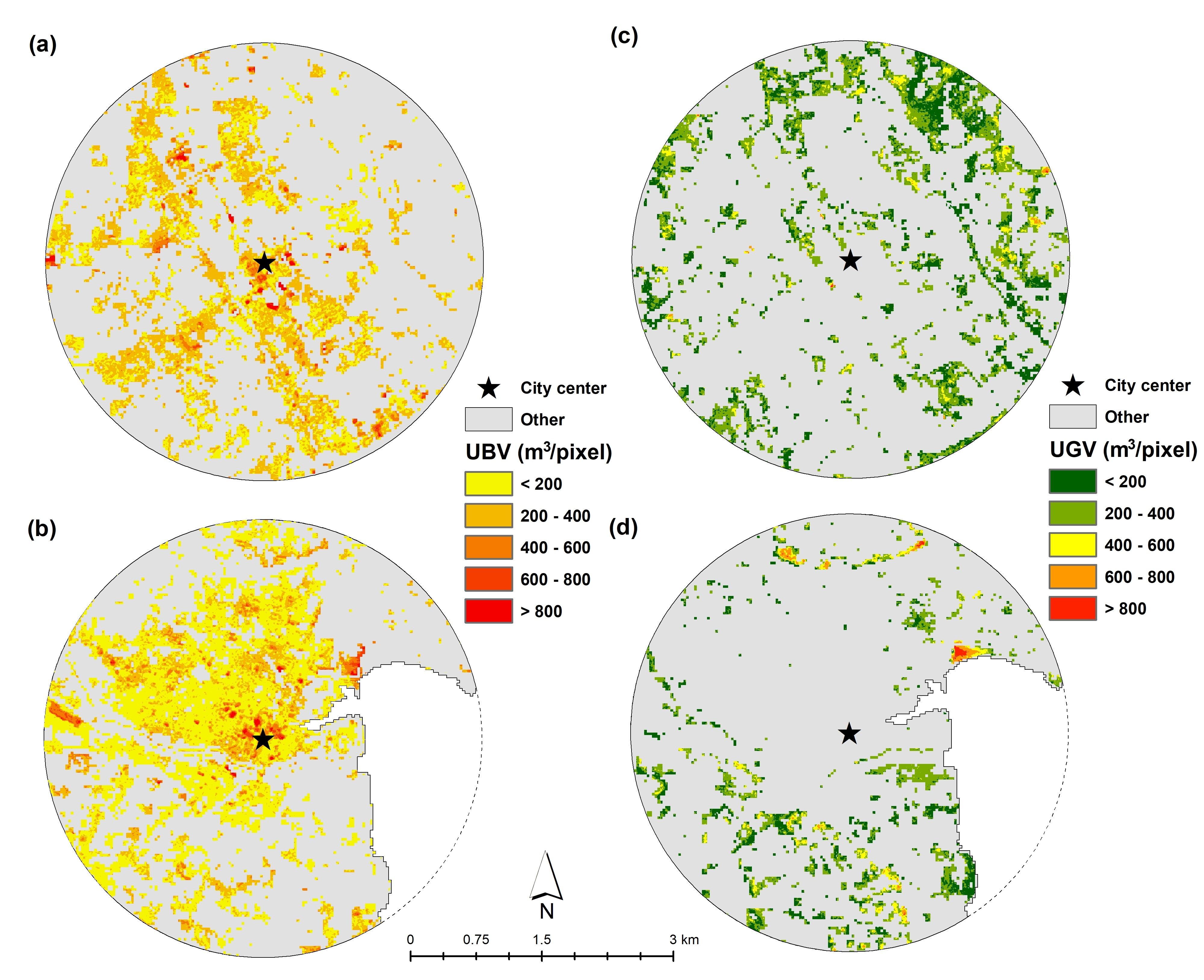
3.1. DTM and SFH in Tsukuba and Tsuchiura

A RMSE of 3.28 m was recorded during the interpolation process. The DTM value ranged from 30.3 m to 69.9 m in Tsukuba and from −3.5 m to 70.9 m in Tsuchiura (Figure 2). Previous research has proven that a larger mesh size produces the actual DTM value rather than the value produced by a smaller mesh size [2,4]. The spatial resolution of ALOS PRISM DSM 5 m was unable to capture ground features less than 25 m2 (playground, less than 5 m wide road, etc.) [4].
A SFH map of both cities with a spatial resolution of 5 m was produced by the subtraction of the DTM from the DSM. The extracted SFH had a value ranging from −11.6 to 93.9 m in Tsukuba and from −10.1 to 73.5 m in Tsuchiura (Figure 2). The negative value was recorded when the DSM was lower than the DTM. The DSM should be greater than or equal to the DTM. Hence, a negative value can be considered as an error. However, the negative value accounted for 0.14% (Tsukuba) and 0.09% (Tsuchiura) of the total pixels. Validation of the SFH was conducted and showed that a RMSE of 6.8 m was achieved. The coefficient of determination (R2) value between the observed and predicted height was 0.78. Previous studies have achieved a RMSE of 7 m [3], and this was the lowest RMSE value recorded in a comparison with other cities, such as Tokyo, Beijing, Shanghai, Surabaya, and Lusaka [3,4].

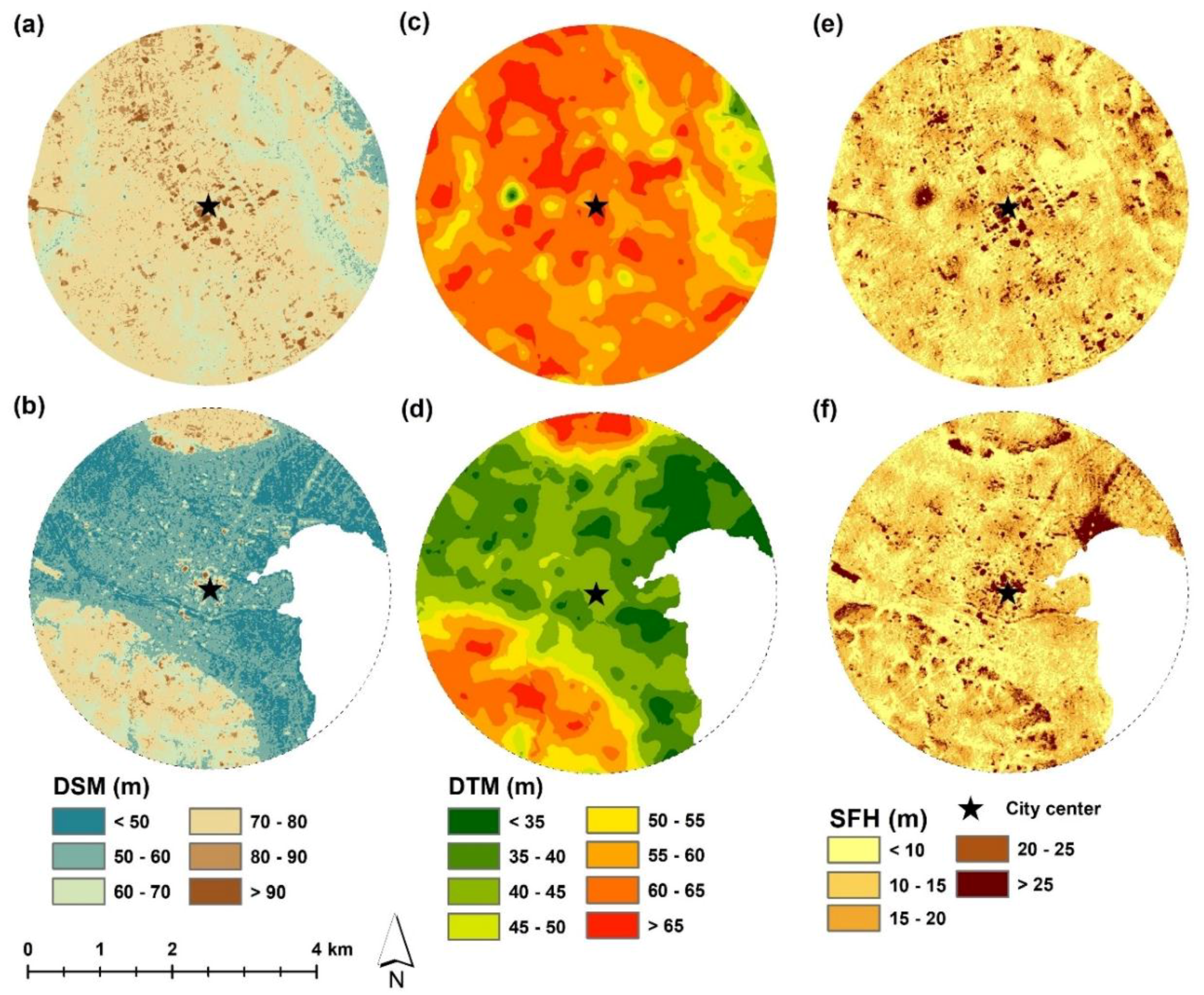
3.2. Land Use/Land Cover and LST Pattern in Tsukuba and Tsuchiura

Figure 3a,b and Table 2 show the land use/land cover map of Tsukuba and Tsuchiura, respectively. Tsuchiura had a higher percentage of built-up area in comparison to Tsukuba. Tsuchiura had a built-up portion of 39.6%, while that of Tsukuba was 27.4%. In Tsuchiura, most of the built-up areas were concentrated in the city core, while in Tsukuba, the built-up areas were scattered.
Tsukuba had more green areas than Tsuchiura during this study period. Tsukuba had a high green percentage of 19.8%, while that of Tsuchiura was only 11.2%. The green areas of Tsukuba were scattered throughout the whole city when compared with those of Tsuchiura. The Tsuchiura green areas were distributed away from the city center. The green areas in Tsukuba were largely distributed in the northern and northeastern part of the city, and the green areas in Tsuchiura were in the southern and southwestern part of the city.

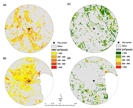
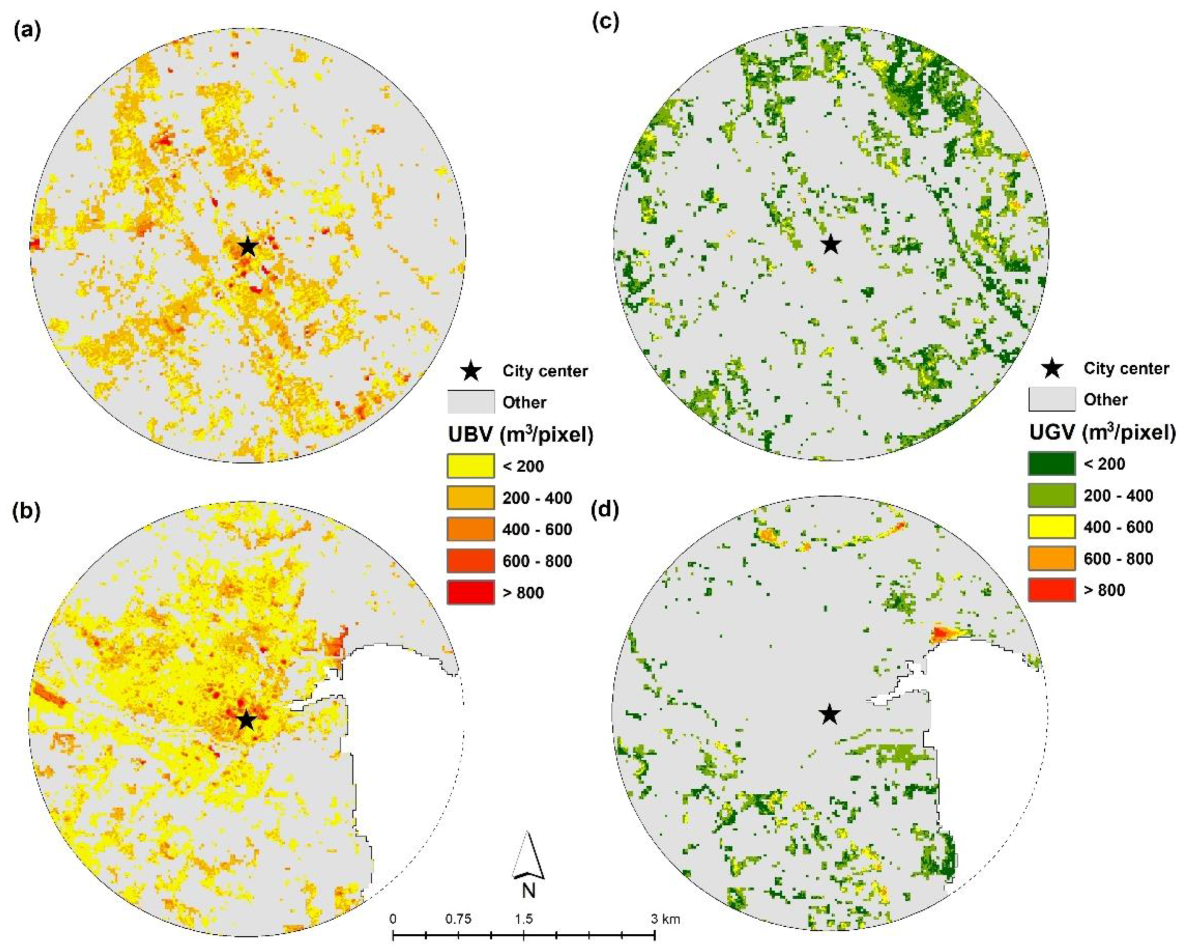
3.3. Estimated UBV and UGV in Tsukuba and Tsuchiura

Figure 4 presents the actual number of the UBV and UGV in m3/pixel corresponding to the 5 m spatial resolution of the DSM. The highest UBV volume was 1658.9 m3/pixel (Figure 4). The total UBV of Tsukuba was approximately 74 million m3. The highest UBV volume of Tsuchiura was 1299.4 m3/pixel. The highest UBV in Tsuchiura was lower than that of Tsukuba. However, the total UBV of Tsuchiura was higher than that of Tsukuba. The total UBV of Tsuchiura was approximately 89 million m3. The UBVs of Tsukuba were scattered, while the built-up areas of Tsuchiura were centered in the city core area. The UBV of Tsukuba was located mostly in the northern, western, and southern parts of the city. In Tsuchiura, more UBV was seen in the northern and western directions of the city. Therefore, urban development policy has been affected by these conditions.
The highest UGV volume was 1144.3 m3/pixel and 1074.1 m3/pixel for Tsukuba and Tsuchiura, respectively (Figure 4). The total UGV of the Tsukuba was higher than that of Tsuchiura. The total UGVs of Tsukuba and that of Tsuchiura were approximately 52 million m3 and 29 million m3, respectively. In the UGV distribution, Tsukuba showed a more scattered pattern than Tsuchiura. Dense UGV of Tsukuba was located in a northern and eastern part of the city, while dense UGV of Tsuchiura was located in the southern part. During the planning process in Tsukuba, the maintenance and control of green areas were considered as part of the urban development [50,51].

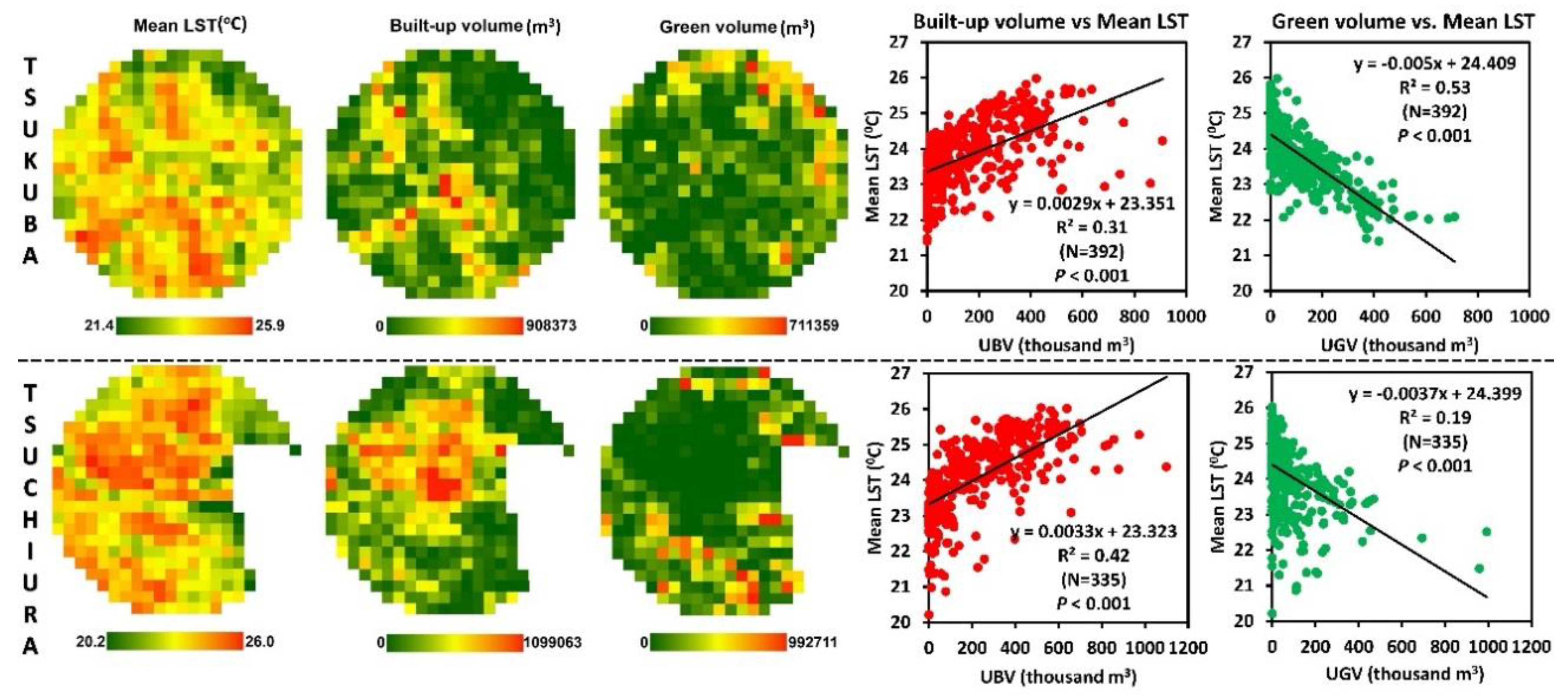
3.4. LST Pattern in Tsukuba and Tsuchiura

Figure 3c,d show the LST maps of Tsukuba and Tsuchiura, respectively. In Tsukuba, the LST ranged from 20.2 °C to 26.4 °C and had a mean value of 23.8 °C. In Tsuchiura, the LST ranged from 19.7 °C to 26.8 °C and had a mean value of 24.1 °C. The highest LST value was identified in the built-up areas of both cities. The lowest LST was recorded in the green space in both cities.
Table 3 shows mean LST difference between the built-up, green space, and other categories. The mean LST was always higher in the built-up areas than in the green spaces for both cities. On the other hand, mean LST of Tsuchiura was higher than that of Tsukuba, which also included the built-up and green areas. The other land use showed a similar mean LST and was recorded as the second highest mean temperature in both cities. The magnitude of mean LST showed that a higher temperature difference could be seen in the built-up and green areas based on the cross-cover comparison in both cities.

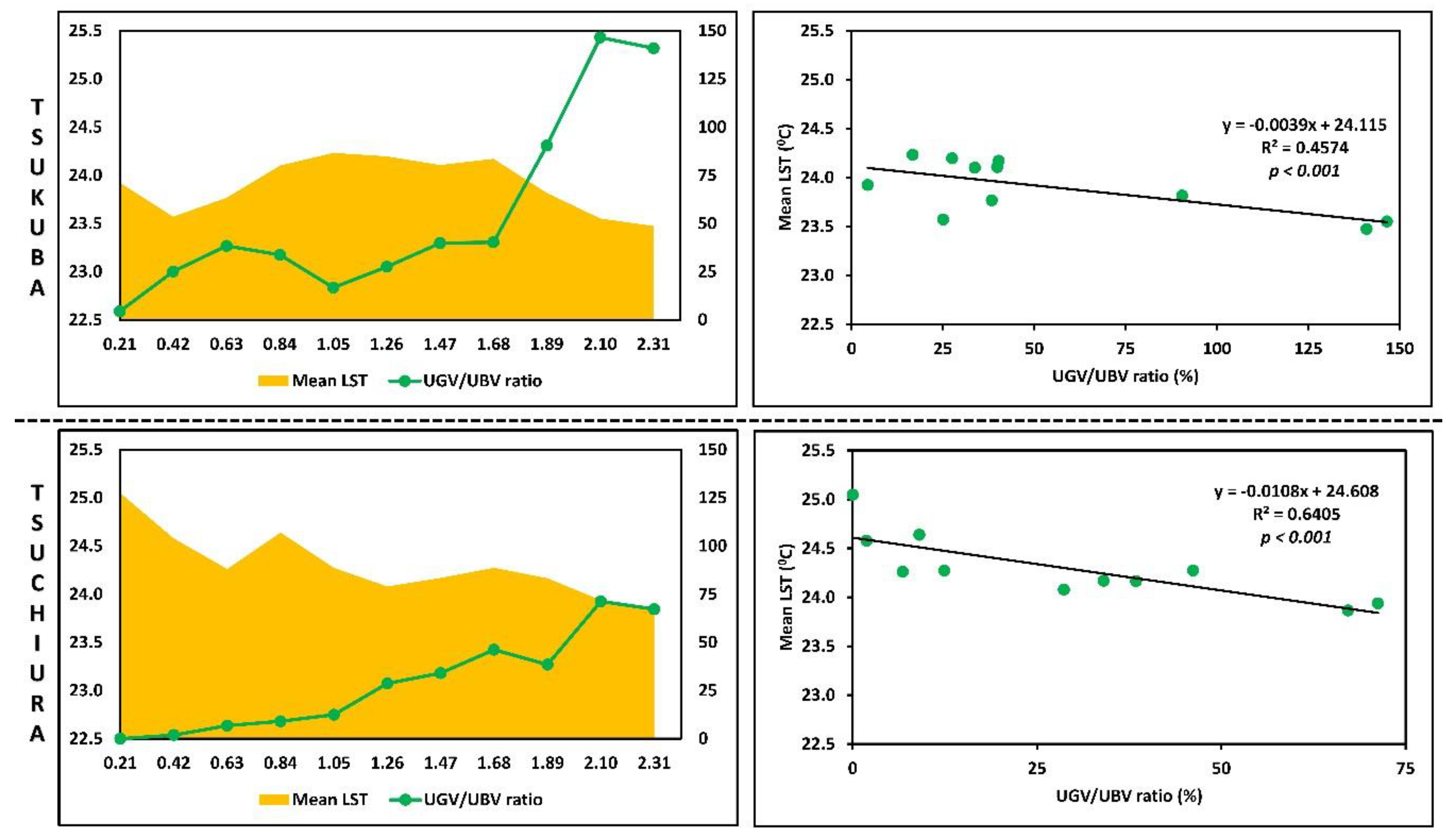
3.5. Urban Spatial Structure with Mean LST

Figure 5 shows the relationship between the total UGV and UBV and mean LST in both cities based on the grid-based method. The UGV had a negative relationship, and the UBV had a positive relationship with mean LST in both cities. A strong relationship between UBV and mean LST was recorded in Tsuchiura, while in Tsukuba, a strong relationship was recorded for UGV and mean LST.
Figure 6 shows the relationship between mean LST and the UGV–UBV ratio along the urban–rural gradients of Tsukuba and Tsuchiura. The UGV–UBV ratio showed that the planned city had a higher percentage than that of the traditionally developed city. For the whole study area, the mean UGV–UBV ratios of 54.9% and 28.7% were recorded for Tsukuba and Tsuchiura, respectively (Table 4).

4. Discussion

As shown in Figure 5, the correlations between the total UGV and UBV and mean LST were statistically significant (p < 0.001) in Tsukuba and Tsuchiura. The correlation was not high for both cities due to the landscape composition. The R2 values for UBV and mean LST were recorded as 0.31 and 0.42 in Tsukuba and Tsuchiura, respectively. The correlation of the two variables was positive for both cities. However, UGV had a negative correlation with mean LST. The R2 values between these two variables were recorded as 0.53 and 0.19 in Tsukuba and Tsuchiura, respectively (Figure 5). This R2 correlation difference was recognized due to the spatial distribution of the UGV and UBV. The total UBV of Tsukuba was 15 million m3 less than that of Tsuchiura. The total UGV of Tsukuba was 23 million m3 greater than that of Tsuchiura.
Our results showed that the UBV and UGV influenced the increase or decrease of the LST. Tsukuba, as a planned city, had a weak positive relationship between UBV and mean LST. However, this planned city had a strong negative relationship between UGV and mean LST when compared with that of the traditionally developed city, Tsuchiura. In planned cities, more attention is given to maintain urban greening, such as green parking lots, urban parks, and trees along the main transportation network. These act to decrease the LST more so than the other land use/land cover categories [23,52]. In comparison, in traditional cities, due to intensive urban development, most green areas have been converted to impervious surfaces (buildings, parking lots, pavement, etc.), which act to increase the LST in urban areas [15,19,53].
The results of our study showed that mean LST of Tsuchiura was always higher than that of Tsukuba. The mean LST was always higher in the built-up areas than in the green areas and other land use categories (Table 3). The spatial distribution of UGV was spread evenly in Tsukuba as a planned city. More green areas could also be identified near the city center (Figure 1e,f). This important distribution directly acted to minimize the LST in Tsukuba. In Tsuchiura, more built-up areas could be recognized inside the city center and the whole study area than in Tsukuba (Figure 3). Built-up areas directly act to increase the LST because of their higher thermal inertia. In contrast, green areas act to decrease the LST based on their low thermal inertia, as they provide shade against sun radiation and generate cool island effects owing to evapotranspiration and emissivity [17,20,54,55].
The impact of urban spatial structure with mean LST was identified by using an urban–rural gradient analysis based on the UGV–UBV ratio of both cities. The UGV–UBV ratio can be considered as an essential indicator of the landscape composition of the cities. The average UGV–UBV ratio was 54.9% and 28.7% for Tsukuba and Tsuchiura, respectively, while the highest ratio was 146.5% and 71.2%, respectively. The UGV–UBV ratio was statistically significant (p < 0.001) and correlated negatively with mean LST in both cities. The R2 value was higher in Tsuchiura than in Tsukuba. This result showed that the entire buffer zone of the traditionally developed city had a higher UBV than UGV. Thus, the UGV–UBV ratio was lower than 100 in Tsuchiura along the entire buffer zone (Table 4). The UGV–UBV ratio of Tsukuba was always higher than that of Tsuchiura in all gradient zones.
According to the results of the study, we showed that the landscape pattern is a vital factor in minimizing the LST in a planned city. In Tsukuba, green spaces have been given a considerable portion of the potential urban development area to maintain urban greening concepts. Tsukuba was developed based on a proper urban planning concept and has been able to maintain 20% of the total areas for green space. As a result of this proper urban plan, Tsukuba is slightly more popular among the educated population than the industrial population. Most of the national-level research institutes are in Tsukuba, and the University of Tsukuba plays a significant role in attracting an educated population into the city area [22,30]. The Tsukuba express railway line helps to minimize the travel time to Tokyo and maintain a level of urban development with a small multicore concept. Thus, most of the facilities are scattered in the Tsukuba periphery. As such, the modern attitude of people also supports the development of Tsukuba as a displaced modern city (Figure 3a and Table 2).
Tsuchiura was developed based on a single-core concept. Most of the hospitals, schools, and other public facilities are inside the CBD area. Therefore, residents need to move to the CBD area to access these facilities. These traditional urban development concepts did not include a proper plan to maintain urban green areas. Thus, more built-up areas are aggregated in the city core, while green areas are distributed away from the city center. This urban development has acted to increase the LST in the city core. In Tsuchiura, the relationship between UBV and mean LST was stronger than the relationship between UGV and mean LST. Accordingly, UBV was more prominent than UGV in its effects on increasing the LST for this traditionally developed city. In addition, the Tsukuba mean LST was lower than that of Tsuchiura in the main land use/land cover categories (built-up and green) as the scattered land use/land cover pattern was directly affected by these differences in both cities.
The UGV–UBV ratio can be used as a proxy indicator to identify the landscape composition of planned and traditionally developed cities. A city developed through a proper plan shows a higher UGV–UBV ratio than that of a traditionally developed city. Past research has shown that 10% of green cover acts to decrease the LST by 0.86 °C [56]. Therefore, the UGV–UBV ratio is much higher in planned cities than in traditionally developed ones. Therefore, the urban policymakers of the Tsuchiura city council need to consider the increase of the UGV near the city areas and maintain a better balance with the UBV. Urban agriculture, green roofs, and green building concepts can be used to maintain the green density. Thus, urban planners can consider more vertical development rather than the traditional horizontal development. This indicator is essential to explain the importance of green volume in a planned city when compared with a traditionally developed city. Urban planners and policymakers need to strongly consider the balance of their UGV–UBV ratio in their future urban planning activities, as a higher ratio can profoundly act to reduce the LST. This article concludes that the measured differences between the two cities are due to the differences in the urban spatial structure between the center city and its form of growth and the modern green city. We suggest that more studies should be performed to confirm the findings of this study.
The analysis in this study only included the 2.5-km buffer radius from both city centers given the availability of the ALOS DSM data. In addition to the UGV and GBV, other environmental factors including wind condition, surface moisture, humidity, and the solar radiation intensity of the two cities could also influence the LST values. Kasumigaura Lake located near Tsuchiura city is calm and quiet with quite low wind speeds. Thus, we ignored the effect of wind on the LST changes. Therefore, it is recommended that the results be interpreted by taking into consideration these limitations. In addition, temporal changes over time were not been examined here and also need to be considered in future studies.

5. Conclusions

In this study, we compared two Japanese cities (Tsukuba and Tsuchiura) using UBV, UGV, mean LST, and the UGV–UBV ratio. The landscape composition directly influenced the spatial pattern of LST in both cities. The total UBV of Tsuchiura was 15 million m3 greater than that of Tsukuba, and the total UGV of Tsukuba was 23 million m3 greater than that of Tsuchiura. Statistical analysis showed that UBV had a positive relationship with mean LST, while UGV had a negative relationship with mean LST in both cities.
In addition, mean LST of Tsuchiura was always higher than that of Tsukuba. The average UGV–UBV ratio was higher in the planned city, Tsukuba, than in the traditionally developed city, Tsuchiura. The UGV–UBV ratio was negatively correlated with mean LST, indicative of the influence of UGV in mitigating the LST. For mean LST difference between built-up area and green space showed that Tsuchiura had 1.8 °C while Tsukuba had 1.7 °C. It can be noted that mean LST difference between built-up area and green space was more intense in the traditional city rather than in the planned city. This can be explained by the difference in urban spatial structure of these two cities.
This study was an attempt to use UBV and UGV for examining the spatial pattern of LST. The planned city Tsukuba, had more green spaces and well-spread (so far) built-up areas than Tsuchiura. This study did not examine the impact of urban planning in detail, and this needs to be considered in future studies.

Author Contributions

Y.M. and R.C.E. proposed the topic. The corresponding author, M.R., spearheaded the data processing and analysis, as well as the writing of the manuscript. R.C.E., H.H.H., X.Z., T.M., T.T., and Y.M. helped in the design, research implementation and analysis, and writing of the manuscript.

Funding

This study was supported by the Japan Society for the Promotion of Science (JSPS) through Grant-in-Aid for Challenging Exploratory Research 16K12816, Scientific Research (B) 18H00763 and ALOS Research and Application Project of EORC, JAXA (6th RA. Geography, No. 3085).

Acknowledgments

The authors would like to express their gratitude to JAXA for providing the ALOS datasets used in this study. The comments and suggestions of the anonymous reviewers are gratefully acknowledged.

Conflicts of Interest

The authors declare no conflict of interest.

References

  1. Koomen, E.; Rietveld, P.; Bacao, F. The third dimension in urban geography: The urban-volume approach. Environ. Plan. B Plan. Des. 2009, 36, 1008–1025. [Google Scholar] [CrossRef]
  2. Estoque, R.C.; Murayama, Y.; Tadono, T.; Thapa, R.B. Measuring urban volume: Geospatial technique and application. Tsukuba Geoenviron. Sci. 2015, 11, 13–20. [Google Scholar]
  3. Estoque, R.C.; Murayama, Y.; Ranagalage, M.; Hou, H.; Subasinghe, S. Validating ALOS PRISM DSM-derived surface feature height: Implications for urban volume estimation. Tsukuba Geoenviron. Sci. 2017, 13, 13–22. [Google Scholar]
  4. Handayani, H.H.; Estoque, R.C.; Murayama, Y. Estimation of built-up and green volume using geospatial techniques: A case study of Surabaya, Indonesia. Sustain. Cities Soc. 2018, 37, 581–593. [Google Scholar] [CrossRef]
  5. Hecht, R.; Meinel, G.; Buchroithner, M.F. Estimation of urban green volume based on single-pulse LiDAR data. IEEE Trans. Geosci. Remote Sens. 2008, 46, 3832–3840. [Google Scholar] [CrossRef]
  6. Naesset, E. Determination of mean tree height of forest stands using airborne laser scanner data. ISPRS J. Photogramm. Remote Sens. 1997, 52, 49–56. [Google Scholar] [CrossRef]
  7. Huang, Y.; Yu, B.; Zhou, J.; Hu, C.; Tan, W.; Hu, Z.; Wu, J. Toward automatic estimation of urban green volume using airborne LiDAR data and high resolution Remote Sensing images. Front. Earth Sci. 2013, 7, 43–54. [Google Scholar] [CrossRef]
  8. Lee, J.H.; Ko, Y.; McPherson, E.G. The feasibility of remotely sensed data to estimate urban tree dimensions and biomass. Urban For. Urban Green. 2016, 16, 208–220. [Google Scholar] [CrossRef] [Green Version]
  9. Giannico, V.; Lafortezza, R.; John, R.; Sanesi, G.; Pesola, L.; Chen, J. Estimating stand volume and above-ground biomass of urban forests using LiDAR. Remote Sens. 2016, 8, 339. [Google Scholar] [CrossRef]
  10. Santos, T.; Rodrigues, A.; Tenedório, J.A. Characterizing urban volumetry using lidar data. Int. Arch. Photogramm. Remote Sens. Spat. Inf. Sci. 2013, XL-4/W1, 29–31. [Google Scholar] [CrossRef]
  11. Lefsky, M.A.; Cohen, W.B.; Acker, S.A.; Parker, G.G.; Spies, T.A.; Harding, D. Lidar remote sensing of the canopy structure and biophysical properties of Douglas-fir western hemlock forests. Remote Sens. Environ. 1999, 70, 339–361. [Google Scholar] [CrossRef]
  12. Holston, J. The Modernist City: An Anthropological Critique of Brasília; University of Chicago Press: Chicago, IL, USA, 1989. [Google Scholar]
  13. Sharifi, A.; Murayama, A. Changes in the traditional urban form and the social sustainability of contemporary cities: A case study of Iranian cities. Habitat Int. 2013, 38, 126–134. [Google Scholar] [CrossRef]
  14. Cervero, R. The planned city: Coping with decentralization: An American perspective. In Proceedings of the Workshop on The planned City, International Conference on “Cities on the Threshold of the 21st Century”, Utrecht University, Netherlands, April 1998; Available online: https://escholarship.org/uc/item/5b29d0fd (accessed on 10 June 2018).
  15. Ranagalage, M.; Estoque, R.C.; Zhang, X.; Murayama, Y. Spatial changes of urban heatisland formation in the Colombo District, Sri Lanka: Implications for sustainability planning. Sustainability 2018, 10, 1367. [Google Scholar] [CrossRef]
  16. Bokaie, M.; Zarkesh, M.K.; Arasteh, P.D.; Hosseini, A. Assessment of urban heat island based on the relationship between land surface temperature and land use/land cover in Tehran. Sustain. Cities Soc. 2016, 23, 94–104. [Google Scholar] [CrossRef]
  17. Estoque, R.C.; Murayama, Y.; Myint, S.W. Effects of landscape composition and pattern on land surface temperature: An urban heat island study in the megacities of Southeast Asia. Sci. Total Environ. 2017, 577, 349–359. [Google Scholar] [CrossRef] [PubMed]
  18. Xiao, R.; Ouyang, Z.; Zheng, H.; Li, W.; Schienke, E.W.; Wang, X. Spatial pattern of impervious surfaces and their impacts on land surface temperature in Beijing, China. J. Environ. Sci. (China) 2007, 19, 250–256. [Google Scholar] [CrossRef]
  19. Ranagalage, M.; Estoque, R.C.; Murayama, Y. An urban heat island study of the Colombo Metropolitan Area, Sri Lanka, based on landsat data (1997–2017). ISPRS Int. J. Geo-Inf. 2017, 6, 189. [Google Scholar] [CrossRef]
  20. Zhang, X.; Estoque, R.C.; Murayama, Y. An urban heat island study in Nanchang City, China based on land surface temperature and social-ecological variables. Sustain. Cities Soc. 2017, 32, 557–568. [Google Scholar] [CrossRef]
  21. Estoque, R.C.; Murayama, Y. Monitoring surface urban heat island formation in a tropical mountain city using Landsat data (1987–2015). ISPRS J. Photogramm. Remote Sens. 2017, 133, 18–29. [Google Scholar] [CrossRef]
  22. Thapa, R.B.; Murayama, Y. Urban mapping, accuracy, & image classification: A comparison of multiple approaches in Tsukuba City, Japan. Appl. Geogr. 2009, 29, 135–144. [Google Scholar] [Green Version]
  23. Onishi, A.; Cao, X.; Ito, T.; Shi, F.; Imura, H. Evaluating the potential for urban heat-island mitigation by greening parking lots. Urban For. Urban Green. 2010, 9, 323–332. [Google Scholar] [CrossRef]
  24. Huang, M.; Cui, P.; He, X. Study of the cooling effects of urban green space in Harbin in terms of reducing the heat island effect. Sustainability 2018, 10, 1101. [Google Scholar] [CrossRef]
  25. Jin, H.; Cui, P.; Wong, N.; Ignatius, M. Assessing the effects of urban morphology parameters on microclimate in singapore to control the urban heat island effect. Sustainability 2018, 10, 206. [Google Scholar] [CrossRef]
  26. Feyisa, G.L.; Dons, K.; Meilby, H. Efficiency of parks in mitigating urban heat island effect: An example from Addis Ababa. Landsc. Urban Plan. 2014, 123, 87–95. [Google Scholar] [CrossRef]
  27. Kardinal Jusuf, S.; Wong, N.H.; Hagen, E.; Anggoro, R.; Hong, Y. The influence of land use on the urban heat island in Singapore. Habitat Int. 2007, 31, 232–242. [Google Scholar] [CrossRef]
  28. Li, Y.Y.; Zhang, H.; Kainz, W. Monitoring patterns of urban heat islands of the fast-growing Shanghai metropolis, China: Using time-series of Landsat TM/ETM+ data. Int. J. Appl. Earth Obs. Geoinf. 2012, 19, 127–138. [Google Scholar] [CrossRef]
  29. Liu, K.; Su, H.; Zhang, L.; Yang, H.; Zhang, R.; Li, X. Analysis of the urban heat Island effect in Shijiazhuang, China using satellite and airborne data. Remote Sens. 2015, 7, 4804–4833. [Google Scholar] [CrossRef]
  30. Murayama, Y. Japanese Urban System. Kluwer Academic Publishers: Dordrecht, The Netherlands, 2000. [Google Scholar]
  31. Tokyo Climate Center. TCC News. 2011, pp. 1–8. Available online: http://ds.data.jma.go.jp/tcc/tcc/news/tccnews25.pdf (accessed on 10 June 2018).
  32. Statistics Bureau, J. Population Data 2017. Statistics Bureau of Japan, Ministry of Internal Affairs and Communication, Japan. Available online: http://www.stat.go.jp/english (accessed on 10 June 2018).
  33. USGS. EarthExplore 2017. Available online: https://earthexplorer.usgs.gov/ (accessed on 1 December 2017).
  34. Tadono, T.; Takaku, J.; Shimada, M. Validation study on Alos Prism Dsm Mosaic and Aster Gdem 2. ISPRS Ann. Photogramm. Remote Sens. Spat. Inf. Sci. 2012, I-4, 193–198. [Google Scholar] [CrossRef]
  35. Japan Aerospace Exploration Agency. ALOS Product Format Description (PRISM); NEC Toshiba Space Systems Ltd: Tsukuba, Japan, 2010. Available online: http://www.ga.gov.au/__data/assets/pdf_file/0017/11717/GA10285.pdf (accessed on 11 June 2018).
  36. Krivoruchko, K. Empirical Bayesian Kriging: Implemented in ArcGIS Geostatistical Analyst. ESRI, 2012. Available online: https://www.esri.com/news/arcuser/1012/files/ebk.pdf (accessed on 10 June 2018).
  37. Xu, H. Modification of normalised difference water index (NDWI) to enhance open water features in remotely sensed imagery. Int. J. Remote Sens. 2006, 27, 3025–3033. [Google Scholar] [CrossRef]
  38. Ji, L.; Zhang, L.; Wylie, B. Analysis of dynamic thresholds for the normalized difference water index. Photogramm. Eng. Remote Sens. 2009, 75, 1307–1317. [Google Scholar] [CrossRef]
  39. Otsu, N. A Threshold selection method from gray-level histograms. IEEE Trans. Syst. Man. Cybern. 1979, 9, 62–66. [Google Scholar] [CrossRef]
  40. Li, W.; Du, Z.; Ling, F.; Zhou, D.; Wang, H.; Gui, Y.; Sun, B.; Zhang, X. A comparison of land surface water mapping using the normalized difference water index from TM, ETM+ and ALI. Remote Sens. 2013, 5, 5530–5549. [Google Scholar] [CrossRef]
  41. Estoque, R.C.; Murayama, Y. Classification and change detection of built-up lands from Landsat-7 ETM+ and Landsat-8 OLI/TIRS imageries: A comparative assessment of various spectral indices. Ecol. Indic. 2015, 56, 205–217. [Google Scholar] [CrossRef]
  42. Zhang, Y.; Odeh, I.O.A.; Han, C. Bi-temporal characterization of land surface temperature in relation to impervious surface area, NDVI and NDBI, using a sub-pixel image analysis. Int. J. Appl. Earth Obs. Geoinf. 2009, 11, 256–264. [Google Scholar] [CrossRef]
  43. Chander, G.; Markham, B.L.; Helder, D.L. Summary of current radiometric calibration coefficients for Landsat MSS, TM, ETM+, and EO-1 ALI sensors. Remote Sens. Environ. 2009, 113, 893–903. [Google Scholar] [CrossRef] [Green Version]
  44. Weng, Q. Thermal infrared remote sensing for urban climate and environmental studies: Methods, applications, and trends. ISPRS J. Photogramm. Remote Sens. 2009, 64, 335–344. [Google Scholar] [CrossRef]
  45. Sobrino, J.A.; Jiménez-Muñoz, J.C.; Paolini, L. Land surface temperature retrieval from LANDSAT TM 5. Remote Sens. Environ. 2004, 90, 434–440. [Google Scholar] [CrossRef]
  46. Weng, Q.; Lu, D.; Schubring, J. Estimation of land surface temperature-vegetation abundance relationship for urban heat island studies. Remote Sens. Environ. 2004, 89, 467–483. [Google Scholar] [CrossRef]
  47. Myint, S.W.; Brazel, A.; Okin, G.; Buyantuyev, A. combined effects of impervious surface and vegetation cover on air temperature variations in a rapidly expanding desert city. GISci. Remote Sens. 2010, 47, 301–320. [Google Scholar] [CrossRef]
  48. Gunaalan, K.; Ranagalage, M.; Gunarathna, M.H.J.P.; Kumari, M.K.N.; Vithanage, M.; Srivaratharasan, T.; Saravanan, S.; Warnasuriya, T.W.S. Application of geospatial techniques for groundwater quality and availability assessment: A case study in Jaffna Peninsula, Sri Lanka. ISPRS Int. J. Geo-Inf. 2018, 7, 20. [Google Scholar] [CrossRef]
  49. Kikon, N.; Singh, P.; Singh, S.K.; Vyas, A. Assessment of urban heat islands (UHI) of Noida City, India using multi-temporal satellite data. Sustain. Cities Soc. 2016, 22, 19–28. [Google Scholar] [CrossRef]
  50. Lambert, B.H. Building Innovative Communities: Lessons from Japan’s Science City Projects; European Institute of Japanese Studies: Stockholm, Sweden, 2000; Volume 107, p. 24. Available online: https://swopec.hhs.se/eijswp/papers/eijswp0107.pdf (accessed on 15 June 2018).
  51. Lee, H.Y. Lessons from Science City Projects and Their Success Factors. Ph.D. Thesis, Massachusetts Institute of Technology, Cambridge, MA, USA, 2002. [Google Scholar]
  52. Ahmed, A.Q.; Ossen, D.R.; Jamei, E.; Manaf, N.A.; Said, I.; Ahmad, M.H. Urban surface temperature behaviour and heat island effect in a tropical planned city. Theor. Appl. Climatol. 2015, 119, 493–514. [Google Scholar] [CrossRef]
  53. Senanayake, I.P.; Welivitiya, W.D.D.P.; Nadeeka, P.M. Remote sensing based analysis of urban heat islands with vegetation cover in Colombo city, Sri Lanka using Landsat-7 ETM+ data. Urban Clim. 2013, 5, 19–35. [Google Scholar] [CrossRef]
  54. Hamada, S.; Ohta, T. Seasonal variations in the cooling effect of urban green areas on surrounding urban areas. Urban For. Urban Green. 2010, 9, 15–24. [Google Scholar] [CrossRef]
  55. Oliveira, S.; Andrade, H.; Vaz, T. The cooling effect of green spaces as a contribution to the mitigation of urban heat: A case study in Lisbon. Build. Environ. 2011, 46, 2186–2194. [Google Scholar] [CrossRef]
  56. Li, X.; Zhou, W.; Ouyang, Z.; Xu, W.; Zheng, H. Spatial pattern of greenspace affects land surface temperature: Evidence from the heavily urbanized Beijing metropolitan area, China. Landsc. Ecol. 2012, 27, 887–898. [Google Scholar] [CrossRef]
Figure 1. Location map of the study areas. (a) Japan; (b) Ibaraki Prefecture; (c) Tsukuba; (d) Tsuchiura (Landsat 5 thematic mapper (TM ) false-color composite bands 4, 3, 2); (e) Tsukuba city center; and (f) Tsuchiura city center based on Google Earth images (420 m × 420 m; 8 May 2010).
Sustainability 10 02366 g001
Figure 2. Advanced Land Observing Satellite panchromatic remote-sensing instrument for stereo mapping digital surface model (ALOS PRISM DSM), digital terrain model (DTM), and surface feature height (SFH) maps of Tsukuba and Tsuchiura: (a) digital surface model (DSM) map of Tsukuba; (b) DSM map of Tsuchiura; (c) DTM map of Tsukuba; (d) DTM map of Tsuchiura; (e) SFH map of Tsukuba; and (f) SFH map of Tsuchiura.
Sustainability 10 02366 g002
Figure 3. Land use/land cover and land surface temperature (LST) maps: (a) land use/land cover map of Tsukuba; (b) land use/land cover map of Tsuchiura; (c) LST map of Tsukuba; and (d) LST map of Tsuchiura.
Sustainability 10 02366 g003
Figure 4. Estimated urban built volume (UBV) and urban green volume (UGV)s (2010): (a) UBV of Tsukuba; (b) UBV of Tsuchiura; (c) UGV of Tsukuba; and (d) UGV of Tsuchiura (Note: The UBV and UGV are presented as real numbers in m3/pixel corresponding to the 5 m spatial resolution of the DSM).
Sustainability 10 02366 g004
Figure 5. Graphical view of the 210 × 210 m polygon grid, showing (Left) the maps of mean LST, total UBV, and total UGV; and (Right) the scatter plots between the UBV and the UGV and mean LST in Tsukuba and Tsuchiura.
Sustainability 10 02366 g005
Figure 6. The relationship between mean LST and the UGV–UBV ratio along the urban–rural gradients of Tsukuba and Tsuchiura.
Sustainability 10 02366 g006
Table 1. Land use/land cover categories in Tsukuba and Tsuchiura.
CategoryIndexThresholding MethodDescription
WaterModified normalized difference water index (MNDWI, Equation (2))Otsu’s optimal binary thresholding [39]All water bodies
Built-upVisible red and near-infrared (NIR)-based built-up index (VrNIR-BI, Equation (3))Manual (Built ≥ − 0.2) All built-up surfaces
Green spaceNormalized difference vegetation index (NDVI) (Equation (4))Manual (Green ≥ 0.495) All green surface
Other (cropland, grassland, bare land, rivers, etc.)Normalized difference vegetation index (NDVI) (Equation (4))Manual (Other < 0.495) All land areas excluding built-up, green surface, and water
Table 2. Land use/land cover percentage area in Tsukuba and Tsuchiura.
Land Use/Land Cover CategoriesTsukuba (%)Tsuchiura (%)
Built-up27.439.6
Green19.811.2
Other (cropland, grassland, bare land, rivers, etc.)52.849.2
Total100100
Table 3. Mean LST of built-up and green space and the magnitude of mean LST (°C).
(a) Mean LST of built-up and green (°C)
Land use/land coverTsukubaTsuchiuraDifference (Tsuchiura − Tsukuba)
Built-up24.524.90.4
Green22.823.10.3
Other23.823.7−0.1
(b) The magnitude and mean LST (°C)
Land use/land cover
(cross-cover comparison)
(∆ mean LST)Difference (Tsuchiura − Tsukuba)
TsukubaTsuchiura
Built-up—Green1.71.80.1
Built-up—Others0.81.10.3
Others—Green1.00.6−0.4
Table 4. UGV–UBV ratio (%) along the urban–rural gradients of Tsukuba and Tsuchiura.
UGV–UBV RatioTsukuba Tsuchiura
Minimum4.40
Maximum146.571.2
Average54.928.7

