The Water Implications of Greenhouse Gas Mitigation: Effects on Land Use, Land Use Change, and Forestry


1
Institute of Development, Southwestern University of Finance and Economics, Chengdu 611130, China
2
Department of Agricultural Economics, Texas A&M University, College Station, TX 77840, USA
*
Author to whom correspondence should be addressed.
Sustainability 2018, 10(7), 2367; https://0-doi-org.brum.beds.ac.uk/10.3390/su10072367
Submission received: 10 June 2018
/
Revised: 22 June 2018
/
Accepted: 4 July 2018
/
Published: 7 July 2018
(This article belongs to the Special Issue Selected Papers on Sustainable Water Resources Management from the 2017 and 2018 International SWAT (Soil and Water Assessment Tool) Conference)
Abstract
:This study addresses the water quantity and quality implications of greenhouse gas mitigation efforts in agriculture and forestry. This is done both through a literature review and a case study. The case study is set in the Missouri River Basin (MRB) and involves integration of a water hydrology model and a land use model with an econometric model estimated to make the link. The hydrology model (Soil and Water Assessment Tool, SWAT) is used to generate a multiyear, multilocation dataset that gives estimated water quantity and quality measures dependent on land use. In turn, those data are used in estimating a quantile regression model linking water quantity and quality with climate and land use. Additionally, a land use model (Forest and Agricultural Sector Optimization Model with Greenhouse Gases, FASOMGHG) is used to simulate the extent of mitigation strategy adoption and land use implications under alternative carbon prices. Then, the land use results and climate change forecasts are input to the econometric model and water quantity/quality projections developed. The econometric results show that land use patterns have significant influences on water quantity. Specifically, an increase in grassland significantly decreases water quantity, with forestry having mixed effects. At relatively high quantiles, land use changes from cropped land to grassland reduce water yield, while switching from cropping or grassland to forest yields more water. It also shows that an increase in cropped land use significantly degrades water quality at the 50% quantile and moving from cropped land to either forest or pasture slightly improves water quality at the 50% quantile but significantly worsens water quality at the 90% quantile. In turn, a simulation exercise shows that water quantity slightly increases under mitigation activity stimulated by lower carbon prices but significantly decreases under higher carbon prices. For water quality, when carbon prices are low, water quality is degraded under most mitigation alternatives but quality improves under higher carbon prices.
1. Introduction
The Intergovernmental Panel on Climate Change (IPCC) [1] indicates greenhouse gas emissions (GHGEs) are a main driver of climate change, and the agriculture and forestry (AF) sector can alter operations to reduce net emissions [2,3,4,5,6,7,8]. The logic for employing AF mitigation involves, among other things, the size of sectoral GHGEs. Estimates indicate AF is the source of 30% of global GHGEs predominately through emissions of methane, nitrous oxide, and carbon dioxide [9]. Additionally, an estimated 25% of historical carbon releases have come from the sectors mainly in the form of lost sequestration [10]. In terms of mitigation, AF can pursue several major types of mitigation actions. First, AF may manipulate enterprise management to reduce cropping-, livestock-, or forest-based emissions. Secondly, AF may enhance sequestration by creating or expanding land-based sinks, retaining more of the carbon that cycling in and out of AF each year. This is done by reducing tillage intensity, altering land use towards less disturbed regimes, reducing deforestation, enhancing forest management, and pursuing afforestation [11,12]. Thirdly, AF may produce substitute products for emission-intensive products like fossil fuels, steel and concrete, displacing emissions involved with their manufacture and use [13]. Finally, AF may develop and utilize technical advances that increase yields while not increasing GHGEs, thus reducing emissions per unit produced and allowing less land to be used to produce a given amount and perhaps less input use [14].
The abovementioned AF mitigation measures have potential co-benefits or adverse side-effects in several dimensions such as institutional, social, economic, or environmental sides [8,15,16]. Specifically, on the environmental side, AF mitigation measures can influence land degradation/restoration, biodiversity, soil quality, and water resources. Here, we focus on water impacts. On balance, a comprehensive study of water quantity and quality effects of a wide array of mitigation possibilities is not available. We attempt to fill that gap.
A number of studies have called for comprehensive examinations of the water effects of mitigation activities. Gupta et al. [17] indicated that many empirical studies of agricultural impacts on water did not account for the fundamental principles of soil water storage, water infiltration, and surface runoff. Medhi et al. [18] argued that combined climate and land use change scenarios should be considered to analyze the impacts of mitigation alternatives on water. Jackson et al. [15] indicate that water quantity effects usually occur through direct alterations in irrigation water use plus alterations in water run off or groundwater infiltration. In general, water quality effects occur when agriculture, forestry, and other land use mitigation strategies alter erosion rates, input usage, and animal manure quantity, in turn altering runoff and infiltration of sedimentation, manure, and chemicals. Others have shown water quality can be improved by use of AF GHGE-mitigating practices like adoption of no till or buffer strips [19,20].
This study does a comprehensive water quality and quantity evaluation of a set of mitigation possibilities in a case study setting. To do this, we employ a hydrological model to simulate water processes coupled with an econometric synthesis and then a land use, economic sector model to incorporate land use change influences. The study is done in the context of the Missouri River Basin (MRB).
2. Literature Based Findings on Mitigation and Water
The following discusses the water quantity and quality implications of AF mitigation strategies under four broad categories: AF management, land use change, bioenergy, and technological progress.
2.1. AF Management
Crop management alternatives for mitigation involve manipulation of tillage, mix of crops grown, irrigation practices, cover crop usage, and fertilization among other possibilities (for an extensive list, see [3,4,21]). Water quantity is affected through: (a) changing tillage practices to retain more residue, which can increase sequestration while also reducing runoff and possibly aquifer infiltration [22]; (b) altering crop mix, like shifting from rice to row crops, which can reduce water diversion, consumption, and evaporation [23,24,25]; and (c) improving irrigation efficiency, which reduces water diversion and evaporative losses plus reduces runoff [26,27]. Also, recharge of groundwater may be increased by additional use of deep tillage [28] but can be reduced because of less intensive conservation tillage [29]. Additionally, when decreasing input intensity, many studies have found that this combined with climate change is likely to decrease water yield but increase water quality [18,30,31].
Mitigation strategies also alter water quality particularly when runoff/infiltration quantity and chemical content are reduced by tillage shifts, reduced fertilization, or conservation practice usage [19,32,33,34,35,36]. For example, Honisch et al. [19] monitored water quality under sustainable farming practices in Bavaria, Germany, finding significant reductions of N loads and phosphate loads after 4 years.
Animal-related mitigation approaches include manure management through digesters and land application, animal stocking intensity/herd size reduction, species choice, grazing land management, and feeding practice alteration. Water quality is affected by use of these practices through changes in runoff of manure, sediments, and nutrients plus indirect cropping effects of altered feed demands. Water quantity is affected by manure handling choice, where systems involving washing increase quantity used and runoff. Fast, mechanical removal of manure solids not only reduces water use but also improves water quality [37,38]. Land-based application of manure as a fertilizer source can increase nutrient runoff and degrade water quality [39,40]. Manipulation of animal stocking intensity/herd size alteration alters manure loads and land runoff potential (by altering vegetative cover), in turn altering water infiltration/runoff and nutrient/sediment runoff. Switches to non ruminant species as opposed to ruminant animal species reduces enteric fermentation while altering feed consumption and the amount of manure produced per unit of animal protein. This in turn affects water quantity and water quality via the means discussed above [41]. Alterations in management of extensive grazing lands can be done via stocking rate reduction, changes in fertilization, improved fire management, reduced brush incidence, and altered plant species mix, all of which in turn alter water infiltration and runoff plus associated sediments and chemicals reaching ground and surface waters.
Forest management mitigation strategies include afforestation, rotation length extension, improved silviculture, and reduced fire incidence, as discussed in Murray et al. [12], Nabuurs et al. [42], and Wall [43]. In terms of water quality, afforestation of crop, pasture, or other land, particularly in the cropland case, could reduce the usage of chemical inputs and soil disturbance, thus reducing chemical runoff and sedimentation and in turn altering water quality [44,45,46]. However, this generally increases the amount of water consumed, as trees use more than grass and crops in many cases [15]. Altering rotation length would reduce sedimentation from soils disturbed by harvesting and alter water quantity through reductions in runoff but increase in vegetative use. Fire management by thinning, removal of dead materials, and controlled burns increase sediment runoff due to soil disturbance but then reduces runoff of ash, nutrients, and sediments when fires occur.
2.2. Land Use Change
Mitigation actions being undertaken to reduce GHGEs would change land use systems [47,48,49,50] and in turn alter water resources. Land use change in an agricultural context involves transformations between cropping, pasture/range, forest, wetlands, or urban spaces. For mitigation, this generally involves movements to less intensive usages, with cropland moving to pasture/range, forestry or wetlands plus pasture moving to forest or wetlands.
Land use change affects water use and water quality with the effect dependent on the original and final land uses along with irrigation status, vegetation mix, and production practices/input use. A number of studies have addressed the water quantity implications of land use change. Leterme and Mallants [51] show that groundwater recharge will increase when cropland is used for maize but will decrease if land is converted to pasture or forest, implying the more complete the land cover, the less the infiltration. Bhardwaj et al. [52] suggest that cropland movement into energy crops will increase water use. Water runoff is also altered when croplands are moved to forests, with runoff predominantly decreasing, indicating that larger plants use more water [15]. Frankenberger [53] examined how runoff is affected by land use in Indiana, finding on fields planted to corn or soybeans that with a 4-in rain, runoff volume fell from 97% to between 12% to 30% when the land was altered to forest, pasture, or turf grass. This is likely due to a combination of these land uses slowing runoff, possibly stimulating more infiltration and increased vegetative water use.
Water quality is also affected by land use [54,55,56,57,58,59]. Erosion is a major force and is altered by mitigation practices that alter tillage intensity or soil disturbance [8,60,61,62,63]. For example, erosion associated with the loss of soil carbon can be reduced by windbreaks, grassland replacement, and afforestation [8,62]. Furthermore, water quality is impacted by rates of chemical or animal manure fertilization [64,65,66]. It is also altered by practices that alter water infiltration, like buffer strips [19,67,68]. The impacts on water quality are varied. For example, Pattanayak et al. [69] and Townsend et al. [70] showed afforestation leading to increased water quality, while Jackson et al. [15] reviewed cases exhibiting the opposite. Thus, impacts on water quantity and quality differ by situation and prior land use/management.
2.3. Bioenergy
Bioenergy is a mitigation alternative with biogenic feedstocks displacing fossil fuel use [2,13]. The same would be true for water, where the direct effects involve water used in processing and production. The Iowa Department of Natural Resources [71] showed quantity can be an issue, with aquifers in Iowa being drawn down by 17.1 ft over 10 years when ethanol facilities were installed.
Quality is also affected as bioenergy feedstock sources include conventional crops and their residues, energy crops, and animal wastes. Raising or recovering such feedstocks can alter runoff of chemical fertilizer, pesticides, and erosion along with vegetative water use and runoff volume [72].
2.4. Technological Progress
Technological progress is another mitigation strategy and can also influence water quantity and quality. This is particularly true when: (1) yield increases are achieved with approximately the same inputs as equal amounts that can be produced with smaller acreage and thus less inputs per unit product; and/or when (2) the same product can be produced with less inputs reducing chemical runoff. For example, recently US corn yields have risen without increasing nitrogen fertilization per acre due to such things as improvements in genetics, pest resistance, drought tolerance, and nutrient efficiency/application practices [14].
Technology can also have quantity impacts when the amount of water used per acre or the land area of crops changes, although this can be either positive or negative. Quality impacts occur when the technological developments induce less input use or crop mix/management shifts that lower chemical input usage and erosion. Baker et al. [14] examined technology effects in a US setting, showing that a continuation of recent trends leads to both reduced GHG emissions and water quality improvements. However, the interrelationship is complex, with many possibilities having different water implications.
3. Empirical Investigation on Mitigation and Water
This study aims to examine the water implications of mitigation strategy use via a four-step process. First, we run a hydrological model (Soil and Water Assessment Tool, SWAT) [73,74] across a broad study region generating results on water quantity and quality. Second, we take the SWAT results and estimate summary equations over them that indicate how land use alters water quantity and quality attributes. Third, we use a land use, economic sector model (the Forest and Agricultural Sector Optimization Model with Greenhouse Gases, hereafter abbreviated as FASOMGHG) [75,76] to simulate land use changes under different mitigation alternatives. Fourth, we evaluate the SWAT summary functions with the FASOMGHG land use changes to examine the composite effects on water. Details on the study area, SWAT use, and climate data follow.
3.1. Study Area
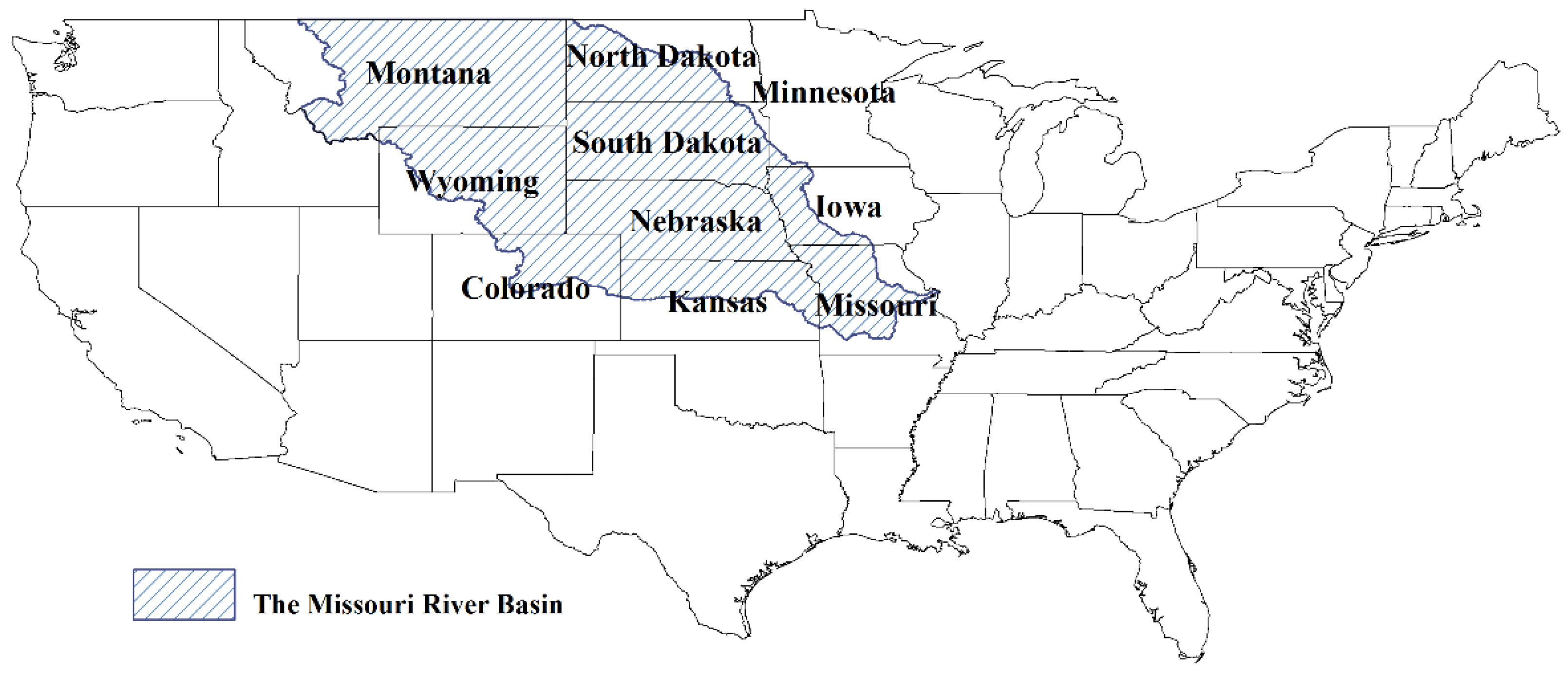
The MRB (Figure 1) is the largest river basin in the continental United States and includes all of Nebraska and parts of Colorado, Iowa, Kansas, Minnesota, Missouri, Montana, North Dakota, South Dakota, and Wyoming, covering a total of 411 counties. The United States Department of Agriculture (USDA) [77] estimates that 29% of the basin land is cropped, 49% is for grazing, 9% is forest, 10% is a mix of permanent pasture, hay land, water, wetland, horticulture, and barren land, and the remaining 3% is urban areas. Most of the grazing land is located in the western and central parts of the basin, while most of the forestland is located in west and central Missouri.
The 2007 Census of Agriculture reported that the MRB produced about $49 billion in agricultural sales, 45% of which is from crops and 55% from livestock. The principal crops grown in the basin are corn, soybeans (mainly in the eastern portion of the basin), and wheat (mainly in the western portion of the basin). Cow calf and feedlot production are the primary livestock enterprises. The USDA [77] indicates that 65% of the cropland was irrigated and 76% of both cropland and pasture were treated with pesticides.
3.2. SWAT Generated Data
To do the estimation phase in this analysis, water information related to land use in MRB is needed. We generated such data using the SWAT model, as it considers many hydrologic processes plus climate, land use, and management practices. SWAT is a comprehensive semi-distributed and physically based model that simulates water quantity and quality within catchments in hydrologic response units (HURs) at a daily time-step [78].
The SWAT input and output data contains records on water runoff, water quality, land use, climate, irrigation water use, and land use change. SWAT input data covers hydrography, terrain, land use, soil, soil drainage-tile, weather, and management practices [74]. SWAT output contains simulated water runoff and water quality indicators on a monthly basis for the 13,437 sub-basins in the MRB. SWAT was run for the 1990–2010 period and is well-calibrated and validated in this study area [79,80].
One estimation focus is water quantity and quality effects. For water quality, following Cude [81], we selected two quality indicators: total nitrogen, including ammonia, nitrate, and nitrite in surface runoff, and total phosphorus in surface runoff, which were rated from 10 to 100. Cude [81] in turn uses a subindex (SI) to convert the water quality indicators into a relative quality rating. The formulae for the total nitrogen and total phosphorus subindices are
- Total Nitrogen (N)
- Total Phosphorus (P)where and are the subindices for the nitrogen- and phosphorus-related measures. A single water quality index (WQI) is then formed from these subindices by using the unweighted harmonic square mean, as in Swamee and Tyagi [82]:where is the water quality index, is the number of subindices, and is the ith subindex.
The SWAT output describes conditions by sub-basin. For the estimation, we aggregated the results to the county level. In doing this, when sub-basins were distributed across several counties, we did a weighted average based on the proportion of each sub-basin that falls within each county.
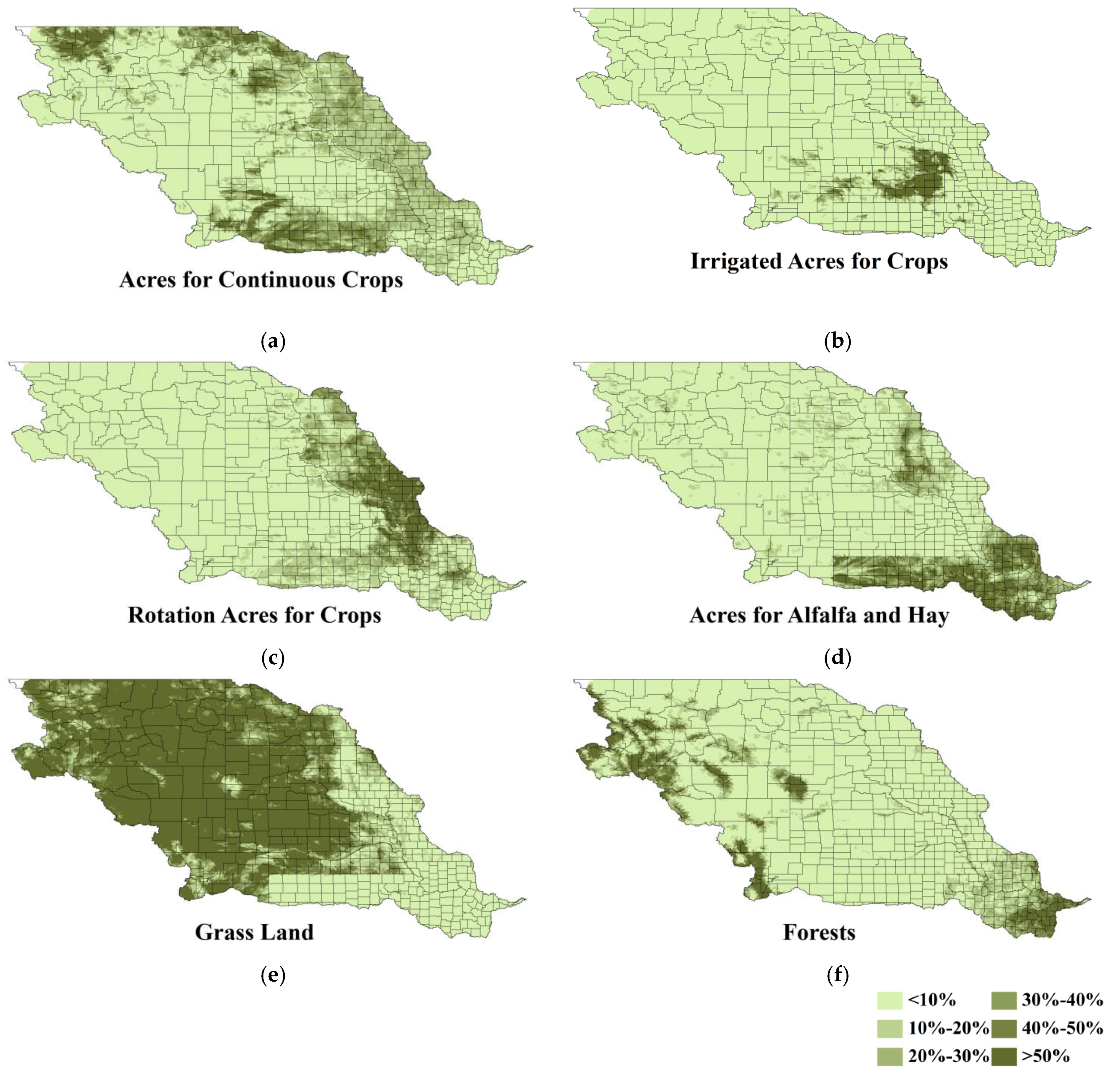
Land use is categorized in SWAT into the following categories: (1) continuous dryland crops, (2) irrigated crops, (3) crop rotations, (4) alfalfa and hay, (5) evergreen forest and deciduous forest, (6) pasture/range, and (7) urban area. In the SWAT simulations, land use is assumed to be time invariant, and Figure 2 portrays the incidence of each land use across the MRB. Although land use does not change over time, the water runoff data was calibrated to real values. In our analysis, we will mainly looked at how land use changes between cropland, grassland, and forest land affect water quality and quantity, and thus we aggregated the cropped lands (categories one to four above) into one broad category: cropped land.
3.3. Climatic Data
Monthly climate data summarizing temperature and precipitation averages and extremes were drawn from the National Oceanic and Atmospheric Administration (NOAA) Satellite and Information Service, National Climatic Data Center (NCDC) for the period 1990–2010 [83]. Those data include: (1) number of days with precipitation greater than or equal to 0.1, 0.5, and 1.0 in, respectively; (2) number of days with minimum temperature less than or equal to 0.0 and 32.0 °F, respectively; (3) number of days with maximum temperature greater than or equal to 90.0 °F; (4) total precipitation measured in millimeters; and (5) monthly mean temperature measured in °F. The NOAA data often contains multiple weather stations in a county and these were averaged across all stations in that county to form the dataset. We also considered the influences of the El Niño Southern Oscillation phase, which is categorized into three phases—warm phase (El Niño), cold phase (La Niña), and neutral phase—as reported by the Japan Meteorological Agency, Tokyo Climate Center [84]. In the period 1990–2010, there were five warm phase years (1991, 1997, 2002, 2006, and 2009) and four cold phase years (1998, 1999, 2007, and 2010).
4. Methods
4.1. Quantile Regression over Panel Data
Quantile regression over panel data [85] was used to summarize SWAT results on how land use affects water runoff quantity and surface water quality. Quantile regression lets us estimate the median and other break points. We estimated 10%, 25%, 50% (median), 75%, and 90% quantiles. The resultant estimation for say the 90% quantile gives a level of water quantity that is exceeded only 10% of the time, with 90% of the observations being equal or smaller.
Quantile regression for panel data following Koenker [85] involves estimating the function
where denotes water quantity or quality measured in region at time and is a vector of independent variables that influence the water quantity and quality (including land use, climate factors, and water quantity (for the quality estimation). are parameters to be estimated, is the regional fixed effect, and is the error term. In terms of the quantiles given, we are estimating quantile , and the conditional τth quantile of is
Following Koenker [85], we can estimate Model (5) for 10 quantiles simultaneously by solving the following minimization problem:
where is the probability weight controlling the relative influence of the associated quantiles and denotes the piecewise linear quantile loss function. Koenker [85] named Problem (6) the penalized quantile regression with fixed effects approach, and we can obtain the fixed effect estimators while λ→0.
4.2. FASOMGHG Model
A national agricultural land use, sector model was used to generate information on mitigation strategies adopted and their land use consequences under alternative mitigation incentives in the form of carbon prices. The model used was FASOMGHG [75,76,86,87], which is a dynamic, nonlinear, and price endogenous programming model of the US forest and agricultural sectors that simulates forest and agricultural land allocation and management over time in a perfectly competitive set of markets. This model represents: forest, crop, and pasture/range land use; agricultural crop and livestock production; livestock feeding; agricultural processing; log production; forest processing; carbon sequestration; CO2/non-CO2 GHG emissions; wood product markets; agricultural markets; and GHG payments [75]. FASOMGHG simulates intertemporal factor and commodity market equilibria which are imposed by the first order conditions resulting from maximizing intertemporal economic welfare. More on the mathematical structure of the model is given in Appendix A and in Adams et al. [75].
In terms of this project, FASOMGHG was run under a range of prices paid per metric ton of GHGEs reduced, sequestered, or offset. In turn, FASOMGHG chose a varying portfolio of agricultural GHG mitigation possibilities composed of manipulations in land use, AF management, and biofuel production across a variety of explicitly modeled sequestration, emission reduction, and biofuels-related possibilities, as done previously by McCarl and Schneider [2], Lee [88], Lee et al. [89], and Murray et al. [12].
5. Estimation Results
As stated above, summary function regressions were estimated over the SWAT county-level results arising from a 1990–2010 simulation. Table 1 reports descriptive statistics on those SWAT water results, the SWAT input data, and the regional climate data. Table 2 reports quantiles in that data for the water quantity yield and water quality. The average water quantity is around 7.2 mm per sub-basin per month, which is close to the value reported at the 75% quantile, meaning that 75% of the SWAT-generated MRB water quantities are below average. On the other hand, the average water quality index is around 19 and we find that 88% of the observations exhibit a lower quality index than that with about half having the worst quality index value (WQI = 10). This shows the importance of examining the whole distribution and is why we used quantile regression.
To begin examination of the interrelationship between land use and water quality, we partitioned the data into different classes based on the water quality index, as shown in Table 3. There, we see that the counties exhibiting the worst water quality have 53.8% of lands being cropped, while those with better water quality have 31.8% of the land cropped. On the other hand, grass coverage in areas exhibiting better water quality averages 40.2%, while it averages 15.7% in areas with the worst water quality. This indicates that land with more grass coverage as opposed to crops tends to have higher water quality, which is not surprising since nitrogen and phosphorus typically are applied on croplands.
We also observe from Table 3 that forest coverage appears to be associated with a slight increase in water quality at the low quantiles but not at the highest forest coverage shares. Furthermore, Table 3 indicates urban coverage worsens water quality. These relationships will be further examined in the econometric analysis.
5.1. Quantile Regression Results for Water Quantity
The quantile regressions are estimated using the R package rqpd [85,90]. Results relevant to the water quantity influence of land use and climate are reported in Table 4.
Land use patterns have significant influences on water quantity across all quantiles. The proportion of land used for crops and forests increases water quantity, but the incremental rate falls as the share of cropland increases, which is in conflict with Molina-Navarro et al. [91]. We also find grass coverage has negative influences on water quantity, with positive effects of squared terms at all quantiles. Urban land positively affects water quantity but only at lower quantiles.
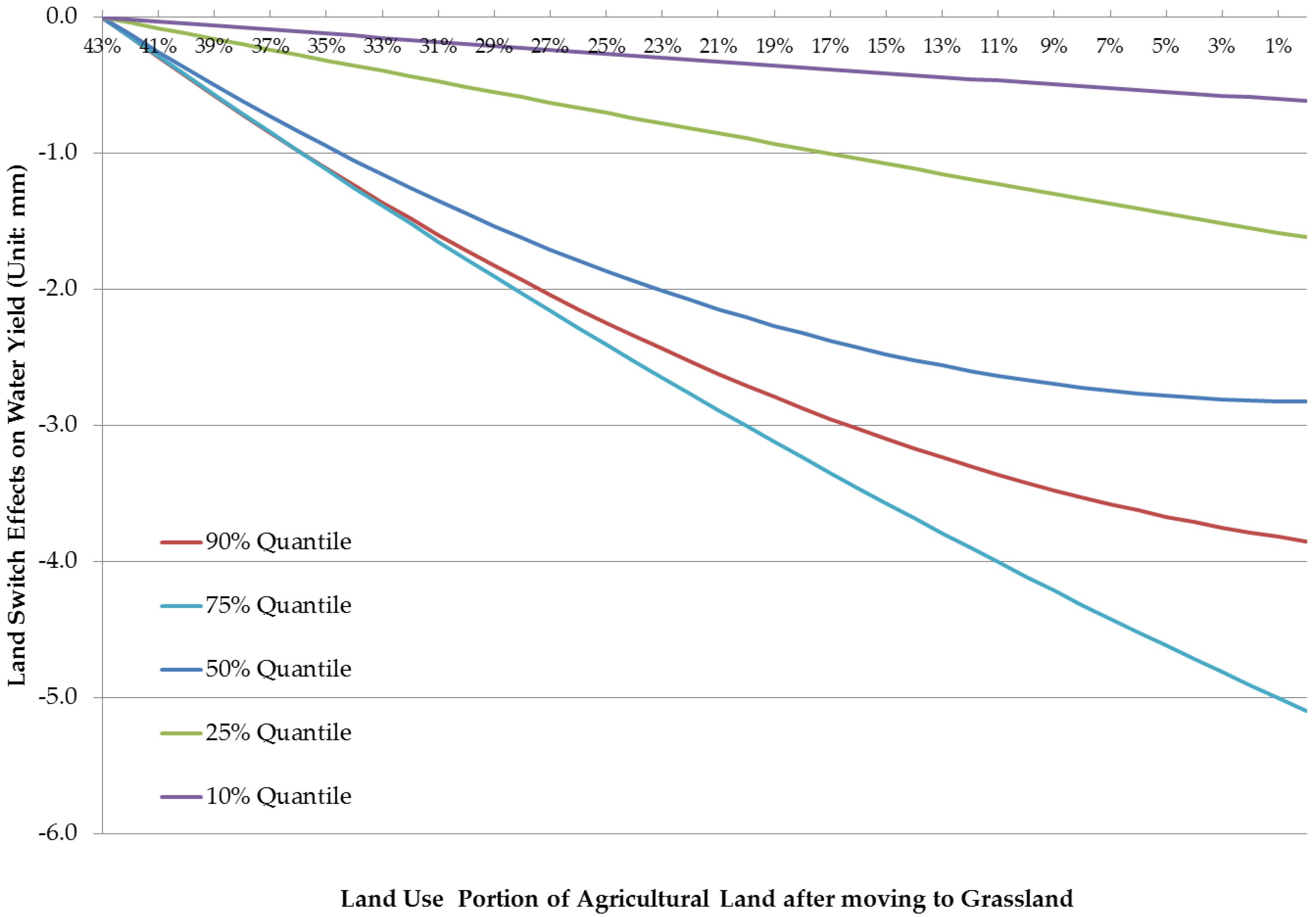
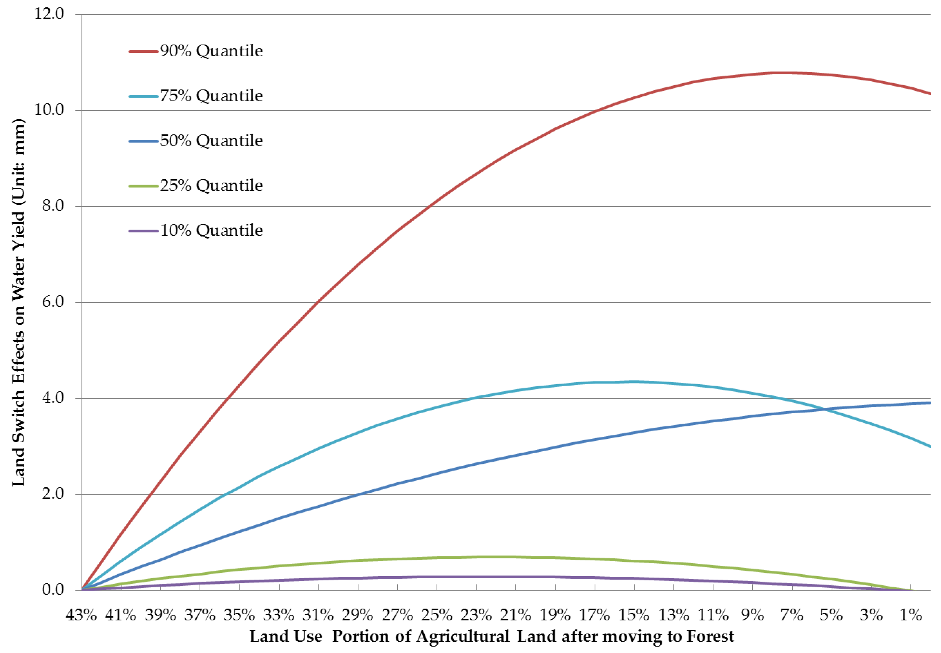
We further calculated land use change effects on water yield. Figure 3, Figure 4 and Figure 5 depict the effects of land reallocations from cropped usage to grassland, from cropped usage to forest, and from grassland to forest, respectively, where other land shares and climate are held constant. The water yield baseline for computing land switch effects is the total water yield under the land shares of 43% cropped land, 28% grassland, and 8% forest—the mean values reported in Table 1.
As land use changes from cropped land to grassland (Figure 3), water quantity reduces at all quantiles, with lower effects at higher quantiles as also found in [51,53]. Namely, when the proportion of cropped land falls from 43% to 32% with a corresponding increase in grassland, then water yield decreases by −1.5 mm at the 75% and 90% quantiles, −1.3 mm at the 50% quantile, −0.4 mm quantile at the 25% quantile, and −0.2 mm at the 10% quantile. It implies that grasslands reduce runoff particularly at relatively high quantiles of water yield. This is likely due to more complete land coverage slowing runoff and increased infiltration.
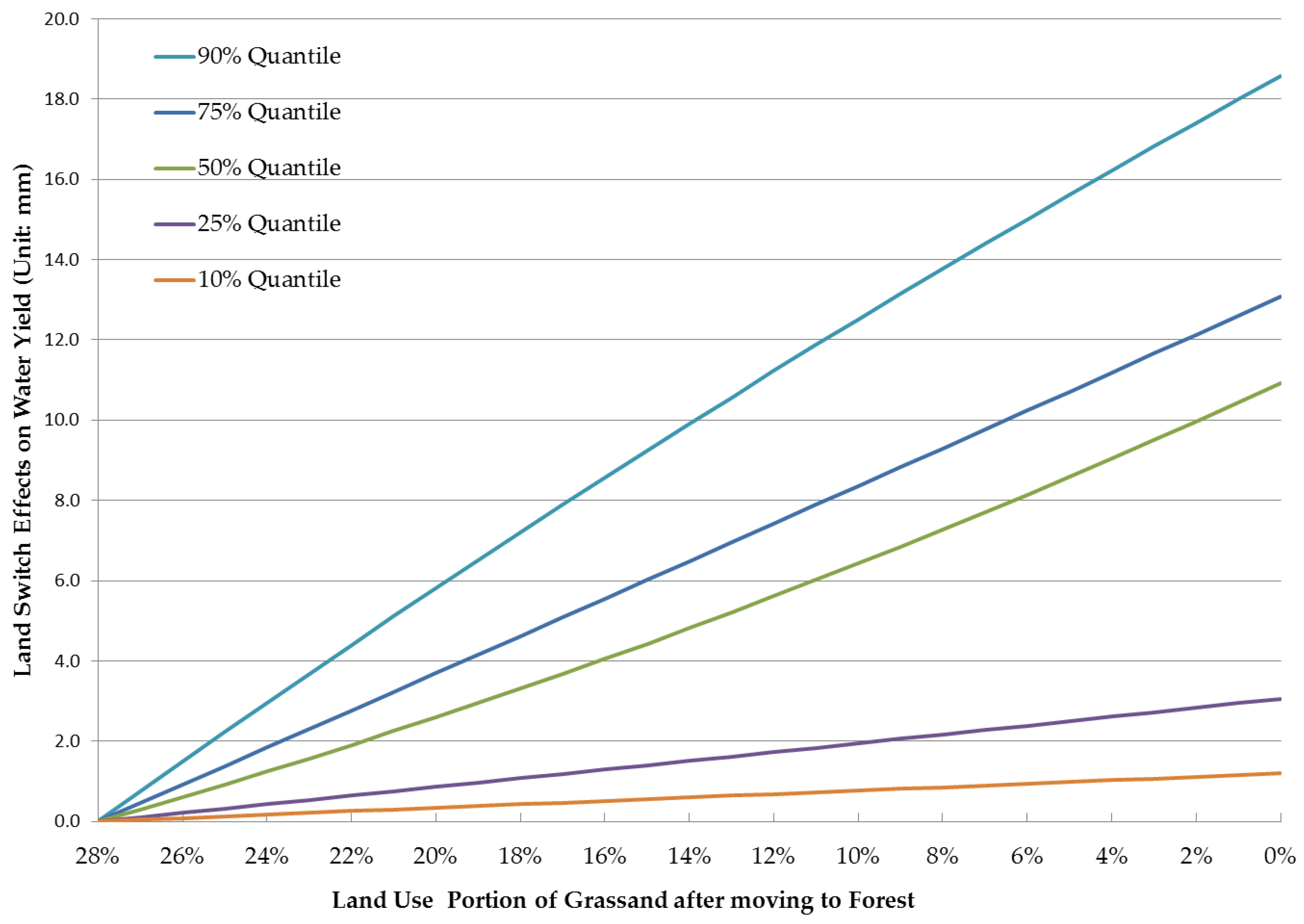
On the other hand, switching land use from cropping to forest (Figure 4) significantly increases water quantity. The result is different from the findings in [15,53]. Moreover, the land switch effects on water yield from cropping to forest takes the form of an inverse U at all quantiles, implying that adding forest land increases water yield up to a critical point then decreases it. Switching from cropping to forest yields more water at the higher quantiles. We also find the same pattern of water yield when grass land switches to forest (Figure 5).
Across these results, afforestation from either cropped land or grassland has greater water quantity benefits than does the switch from cropped land to grassland.
On the climate side, the results show, unsurprisingly, that water quantity is principally influenced by precipitation, with increases as conditions get wetter. Also, a measure of precipitation extremes (the number of days with greater than 1 in of precipitation) is also associated with increased quantity, a result that conflicts with the findings in Zhang et al. [92]. Average temperature, on the other hand, does not have significant effects across most quantile equations but extreme temperature events do. The number of cold days (≤32 °F) has a positive effect on water quantity, while the number of hot days (≥90 °F) has a negative impact.
On El Niño and La Niña events, we find El Niño reduces MRB water quantity while La Niña increases it at all quantiles. This corresponds with NOAA findings that MRB winters are warmer and drier when El Niño occurs, while La Niña leads to cooler and wetter winters [93]. The results also show that both El Niño and La Niña have greater effects on the higher quantiles.
5.2. Quantile Regression Results for Water Quality
Water quality quantile regressions are given in Table 5, although we had to drop the 10% quantile since almost all of observations in that quantile exhibit the lowest water quality value of 10. Additionally, most of the estimated coefficients are insignificant in the 25% and 75% quantiles, so we mainly discuss the land use impacts on the 50% and 90% quantiles.
Previous studies have found that agricultural land use has impacts on water quality [94,95,96], while Sliva and Williams [97] found the opposite. In our analysis, the results show that moving from cropped land to either forest or pasture will slightly improve water quality at the 50% quantile but worsen water quality at the 90% quantile. An increase in cropped land use significantly degrades water quality at the 50% quantile. Previous studies have found that water quality is strongly influenced by agricultural land use and land use change [44,59,91,95,96,98]. For example, Lee et al. [59] found that the proportions of land use of urban, agricultural, and forest are correlated with water quality in South Korea. Gunawardhana et al. [98] found that converting forested land to agricultural land degrades water quality in the Uma Oya catchment area in Sri Lanka. Miserendino et al. [99] and Tu [100] found that water quality increases as forest land increases, perhaps because of lower inorganic ions in forested land use [56,58,97,101]. Urban area does not have significant impacts on water quality, which conflicts with the results from the study of DeFries and Eshleman [57], Miserendino et al. [99], and Ahearn et al. [102].
The effect of water quantity on water quality is positive at the 90% quantile but negative at the 75% quantile. The quantity effect on water quality at the 75% quantile is negative and similar to results at the 50% quantile, and it implies that increasing water quantity will improve the higher part of the water quality distribution (WQI > 90% quantile) but worsen lower water quality below that (WQI < 75% quantile), perhaps due to runoff. Our result is consistent with Molina-Navarro et al. [91] at higher quantiles in showing that water quality is closely linked with water quantity.
Next, we discuss the impacts of climatic factors. Notice that the impacts depend on current conditions since the estimated functions include squared terms for some climate variables. The result shows that water quality will worsen with lower precipitation levels and is improved as precipitation increases. Extreme precipitation has positive impacts on water quality probably since precipitation has dilution and flushing effects. On the other hand, extreme temperature degrades water quality. This is likely because extreme lower temperatures freeze water and slow down flows while extreme high temperatures cause higher evaporation or transpiration, in turn reducing water flows and resultant dilution.
The marginal effects from El Niño and La Niña have opposite results between the 50% and 90% quantiles, with the absolute magnitude at the 90% quantile being larger than that at the 50% quantile. Compared with the neutral phase, El Niño and La Niña significantly improve water quality at the 90% quantile, while both El Niño and La Niña have significant negative effects on water quality at the 50% quantile.
6. Analysis of Water Implications of Mitigation Strategy Choice
We now turn to examine the effects of mitigation efforts on water quantity and quality. We do this by using FASOMGHG model under different carbon prices to give us changes in: (1) afforestation; (2) crop fertilization; (3) crop tillage intensification; (4) crop management; (5) livestock enteric and manure management; (6) bioenergy feedstock incidence; and (7) forest management. The afforestation mitigation strategy converts crop and/or grasslands to forest, and the forest management strategy includes lengthened timber rotations, increased forest management intensity, and avoided deforestation. In simulating the effects at different carbon prices, we ran FASOMGHG one strategy at a time and later allowed the whole portfolio of strategies.
The runs were done under several hypothetical carbon price scenarios which contained rising prices. Specifically, the prices were initially set at $5, $10, $30, and $50 per metric ton CO2 equivalent but then escalated at 5% per year. Additionally, we ran a baseline scenario with no carbon price. The considered shifts in land use were those under the carbon price scenario relative to those under the baseline scenario.
The version of FASOMGHG used has the conterminous United States divided into 11 regions. The Missouri River Basin consists of parts of the FASOMGHG regions of the Corn Belt, Northern Plains, and Rocky Mountains, and based on land use shares, we used 10.90% of the Corn Belt results, 45.72% of the Northern Plains, and 43.38%, of the Rocky Mountains.
FASOMGHG generated many results, but here, we will only focus on those with implications for water. The FASOMGHG results for cropped land, grassland, and forested land plus the regression evaluations for the 50% quantile are reported in Table 6. All the values use simulated land use changes during the five-year period beginning with 2025.
6.1. Effects under the Lower Carbon Price Scenarios
The first carbon price scenario—$5 at a 5% increase—shows that in all of the single strategy mitigation runs, excepting the bioenergy case, there is a small increase in cropped land with an accompanying decrease in both grassland and forest land. When carbon prices are only paid for crop fertilization reduction, the results show cropped land use increases by 0.83%, while grassland and forests decrease by 0.78% and 0.16%, causing an increase in water quantity and a decrease in water quality. The opposite effects occur for bioenergy, forest management, and the case where all strategies are allowed with water quantity decreasing but quality increasing. Similar results are found under the $10 at a 5% increase carbon price scenario. There, all the single strategy mitigation cases expand cropping but reduce grassland and forests.
6.2. Effects under the Higher Carbon Price Scenarios
In the higher carbon price scenarios (those starting with $30 and $50 prices), all the single strategy mitigation results and the simultaneous case decrease cropping and forests but increase grassland. In these scenarios, water quantity is decreased while water quality increases across the board. When forest management is the only available strategy, this causes the largest water quantity decrease and water quality increase across the individual strategies. The all strategies case causes yet a larger quantity reduction (1.05 mm per acre in the $30 case) and the largest increase in water quality. This suggests that stronger AF mitigation efforts will result in reduced water quantity but increased water quality. We also see diminishing effects on quantity and quality as prices go higher.
7. Conclusions
This paper reports water quality and quantity implications of agricultural and forestry climate change mitigation strategies. To do this, we did an empirical study in the Missouri River Basin investigating the effects of differing levels of mitigation incentives and involving four phases.
First, we ran SWAT for 21 years, observing water quantity and quality effects on a monthly basis for the 13,437 hydrologic unit watershed levels. Then, we took those results and aggregated them to counties, in turn, doing a quantile regression estimation over panel data explaining the water quantity and quality effects of altered land use shares and climate. The result shows that an increase in grassland significantly decreases water quantity but increases quality, while changes in cropped land share have the opposite effect. We also found an increase in forested land share had mixed effects.
The third empirical phase examined the land use effects of an agricultural and forestry mitigation strategy adopted under alternative carbon prices. The fourth phase integrated the quantile regressions and the land use effects to project water quantity and quality effects of various carbon prices and mitigation strategies. The consequent results showed crop fertilization, afforestation, and livestock strategies generally led to increased water quantity and decreased quality under lower carbon price scenarios but led to the opposite result under higher carbon price scenarios. The results also showed that water quality is degraded under most mitigation alternatives except for the production of bioenergy feedstocks and the alteration of forest management. In these cases, these effects occurred when carbon price was low but was reversed with higher carbon prices.
Collectively, the results imply that AF mitigation has varied effects on water quantity and water quality, depending on the carbon price or the extent of mitigation activity. Generally, water quantity is slightly increased under lower carbon prices but then is reduced when carbon prices go higher. Water quality results reveal mixed effects at lower prices but an improvement under higher carbon prices. We also see the magnitudes of improvement shrink as the carbon price goes higher.
Author Contributions
B.A.M. had the original idea for the study and conducted literature review; C.-H.Y. collected data and carried out the analyses; both authors shared in drafting the manuscript, and both approve the final version.
Acknowledgments
The authors would like to thank R. Srinivasan and Prasad Daggupati for providing data from simulations with the SWAT model.
Conflicts of Interest
The authors declare no conflict of interest.
Appendix A
The FASOMGHG mathematical structure is summarized below and treated in depth in Adams et al. [75]. The model embodies the following assumptions: (1) there are h commodities including row (primary) and processed (secondary) products produced by firms, which use inputs and resources in production processes; (2) the aggregate market is simulated by the optimization problem, which seeks to maximize the discounted sum of consumers’ and producers’ surpluses over time and discount rate ; and (3) the optimization problem is subject to demand supply balances and resource restrictions.
Based on the above assumptions, the set of equations of FASOMGHG are as follows:
where , , and refer to the consumed quantity of commodities, the level of production processes, the purchased quantities of inputs, and the resource endowments, respectively. The coefficients , , and depict the quantitative relationships among these variables. Then, the maximand (5) is the net present value of welfare; (3) balances commodities sold with production; (7) balances purchased inputs with use; (8) limited fixed quantities of land and water; and (8) imposes non-negativity.
References
- Pachauri, R.K.; Allen, M.R.; Barros, V.R.; Broome, J.; Cramer, W.; Christ, R.; Church, J.A.; Clarke, L.; Dahe, Q.; Dasgupta, P. Climate Change 2014: Synthesis Report. Contribution of Working Groups I, II to the Fifth Assessment Report of the Intergovernmental Panel on Climate Change; Cambridge University Press: Cambridge, UK; New York, NY, USA, 2014. [Google Scholar]
- McCarl, B.A.; Schneider, U.A. US agriculture’s role in a greenhouse gas emission mitigation world: An economic perspective. Rev. Agric. Econ. 2000, 22, 134–159. [Google Scholar] [CrossRef]
- Kindermann, G.; Obersteiner, M.; Sohngen, B.; Sathaye, J.; Andrasko, K.; Rametsteiner, E.; Schlamadinger, B.; Wunder, S.; Beach, R. Global cost estimates of reducing carbon emissions through avoided deforestation. Proc. Natl. Acad. Sci. USA 2008, 105, 10302–10307. [Google Scholar] [CrossRef] [PubMed] [Green Version]
- Smith, P.; Martino, D.; Cai, Z.; Gwary, D.; Janzen, H.; Kumar, P.; McCarl, B.A.; Ogle, S.M.; O’Mara, F.; Rice, C.; et al. Greenhouse Gas Mitigation in Agriculture. Philos. Trans. R. Soc. B Biol. Sci. 2008, 363, 789–813. [Google Scholar] [CrossRef] [PubMed]
- Golub, A.; Hertel, T.; Lee, H.L.; Rose, S.; Sohngen, B. The opportunity cost of land use and the global potential for greenhouse gas mitigation in agriculture and forestry. Resour. Energy Econ. 2009, 31, 299–319. [Google Scholar] [CrossRef] [Green Version]
- Smith, P.; Bustamante, M.; Ahammad, H.; Clark, H.; Dong, E.A.; Elsiddig, H.; Haberl, R.; Harper, J.; House, J.; Jafari, M.; et al. Agriculture, Forestry, Forestry and Other Land Use (AFOLU). In Climate Change 2014: Mitigation of Climate Change. Contribution of Working Group III to the Fifth Assessment Report of the Intergovernmental Panel on Climate Change; Cambridge University Press: Cambridge, UK; New York, NY, USA, 2014. [Google Scholar]
- Rose, S.K.; Ahammad, H.; Eickhout, B.; Fisher, B.; Kurosawa, A.; Rao, S.; Riahi, K.; van Vuuren, D.P. Land-based mitigation in climate stabilization. Energy Econ. 2012, 34, 365–380. [Google Scholar] [CrossRef]
- Bustamante, M.; Robledo-Abad, C.; Harper, R.; Mbow, C.; Ravindranat, N.H.; Sperling, F.; Haberl, H.; Siqueira Pinto, A.; Smith, P. Co-benefits, trade-offs, barriers and policies for greenhouse gas mitigation in the agriculture, forestry and other land use (AFOLU) sector. Glob. Chang. Biol. 2014, 20, 3270–3290. [Google Scholar] [CrossRef] [PubMed] [Green Version]
- IPCC. Climate Change 2007: Mitigation: Contribution of Working Group III to the Fourth Assessment Report of the Intergovernmental Panel on Climate Change; Metz, B., Davidson, O.R., Bosch, P.R., Dave, R., Meyer, L.A., Eds.; Cambridge University Press: Cambridge, UK; New York, NY, USA, 2007. [Google Scholar]
- Ruddiman, W.F. The anthropogenic greenhouse era began thousands of years ago. Clim. Chang. 2003, 61, 261–293. [Google Scholar] [CrossRef]
- Lal, R. Soil carbon sequestration impacts on global climate change and food security. Science 2004, 304, 1623–1627. [Google Scholar] [CrossRef] [PubMed]
- Murray, B.C.; Sohngen, B.; Sommer, A.; Depro, B.; Jones, K.; McCarl, B.A.; Gillig, D.; de Angelo, B.; Andrasko, K. Greenhouse Gas Mitigation Potential in US Forestry and Agriculture; Environmental Protection Agency, Office of Atmospheric Programs: Washington, DC, USA, 2005.
- McCarl, B.A. Bioenergy in a greenhouse mitigating world. Choices 2008, 23, 31–33. [Google Scholar]
- Baker, J.S.; Murray, B.C.; McCarl, B.A.; Feng, S.J.; Johansson, R. Implications of alternative agricultural productivity growth assumptions on land management, greenhouse gas emissions, and mitigation potential. Am. J. Agric. Econ. 2013, 95, 435–441. [Google Scholar] [CrossRef]
- Jackson, R.B.; Jobbágy, E.G.; Avissar, R.; Roy, S.B.; Barrett, D.; Cook, C.W.; Farley, K.A.; Le Maitre, D.C.; McCarl, B.A.; Murray, B.C. Trading water for carbon with biological carbon sequestration. Science 2005, 310, 1944–1947. [Google Scholar] [CrossRef] [PubMed]
- Elbakidze, L.; McCarl, B.A. Sequestration offsets versus direct emission reductions: Consideration of environmental co-effects. Ecol. Econ. 2007, 60, 564–571. [Google Scholar] [CrossRef]
- Gupta, S.C.; Kessler, A.C.; Brown, M.K.; Zvomuya, F. Climate and agricultural land use change impacts on streamflow in the upper midwestern United States. Water Resour. Res. 2015, 51, 5301–5317. [Google Scholar] [CrossRef] [Green Version]
- Mehdi, B.; Lehner, B.; Gombault, C.; Michaud, A.; Beaudin, I.; Sottile, M.F.; Blondlot, A. Simulated impacts of climate change and agricultural land use change on surface water quality with and without adaptation management strategies. Agric. Ecosyst. Environ. 2015, 213, 47–60. [Google Scholar] [CrossRef]
- Honisch, M.; Hellmeier, C.; Weiss, K. Response of surface and subsurface water quality to land use changes. Geoderma 2002, 105, 277–298. [Google Scholar] [CrossRef]
- Lal, R.; Delgado, J.A.; Groffman, P.M.; Millar, N.; Dell, C.; Rotz, A. Management to mitigate and adapt to climate change. J. Soil Water Conserv. 2011, 66, 276–285. [Google Scholar] [CrossRef] [Green Version]
- Mehdi, B.B. Scenarios and Implications of Land Use and Climate Change on Water Quality in Mesoscale Agricultural Watersheds. Ph.D. Thesis, McGill University, Montreal, QC, Canada, 2014. [Google Scholar]
- Holland, J.M. The environmental consequences of adopting conservation tillage in Europe: Reviewing the evidence. Agric. Ecosyst. Environ. 2004, 103, 1–25. [Google Scholar] [CrossRef]
- Yagi, K.; Tsuruta, H.; Kanda, K.; Minami, K. Effect of water management on methane emission from a Japanese rice paddy field: Automated methane monitoring. Glob. Biogeochem. Cycles 1996, 10, 255–267. [Google Scholar] [CrossRef]
- Sadras, V.O.; Grassini, P.; Steduto, P. Status of Water Use Efficiency of Main Crops. 2011. Available online: http://www.fao.org/fileadmin/templates/solaw/files/thematic_reports/TR_07_web.pdf (accessed on 16 September 2016).
- Carey, M.; Baraer, M.; Mark, B.G.; French, A.; Bury, J.; Young, K.R.; McKenzie, J.M. Toward hydro-social modeling: Merging human variables and the social sciences with climate-glacier runoff models (Santa River, Peru). J. Hydrol. 2014, 518, 60–70. [Google Scholar] [CrossRef]
- Perry, C. Efficient irrigation; inefficient communication; flawed recommendations. Irrig. Drain. 2007, 56, 367–378. [Google Scholar] [CrossRef] [Green Version]
- Pfeiffer, L.; Lin, C.C. Does efficient irrigation technology lead to reduced groundwater extraction? empirical evidence. J. Environ. Econ. Manag. 2014, 67, 189–208. [Google Scholar] [CrossRef]
- Raper, R.L. Subsoiling. In Encyclopedia of Soils in the Environment; Hillel, D., Ed.; Elsevier Ltd.: Oxford, UK, 2004; pp. 69–76. ISBN 9780123485304. [Google Scholar]
- Pikul, J.L.; Aase, J.K. Water infiltration and storage affected by subsoiling and subsequent tillage. Soil Sci. Soc. Am. J. 2003, 67, 859–866. [Google Scholar] [CrossRef]
- Wu, L.; Long, T.Y.; Liu, X.; Guo, J.S. Impacts of climate and land-use changes on the migration of non-point source nitrogen and phosphorus during rainfall-runoff in the Jialing River Watershed, China. J. Hydrol. 2012, 475, 26–41. [Google Scholar] [CrossRef]
- El-Khoury, A.; Seidou, O.; Lapen, D.R.; Que, Z.; Mohammadian, M.; Sunohara, M.; Bahram, D. Combined impacts of future climate and land use changes on discharge, nitrogen and phosphorus loads for a Canadian river basin. J. Environ. Manag. 2015, 151, 76–86. [Google Scholar] [CrossRef] [PubMed]
- Beasley, R.P. Erosion and sediment pollution control. In Erosion and Sediment Pollution Control; Iowa State University Press: Ames, Iowa, 1972; ISBN 19730707036. [Google Scholar]
- Moldenhauer, W.C.; Langdale, G.W.; Frye, W.; McCool, D.K.; Papendick, R.I.; Smika, D.E.; Fryrear, D.W. Conservation tillage for erosion control. J. Soil Water Conserv. 1983, 38, 144–151. [Google Scholar]
- Ongley, E.D. Control of Water Pollution from Agriculture; Food & Agriculture Organization of the United Nations: Rome, Italy, 1996. [Google Scholar]
- Bjorneberg, D.L.; Westermann, D.T.; Aase, J.K. Nutrient losses in surface irrigation runoff. J. Soil Water Conserv. 2002, 57, 524–529. [Google Scholar]
- Rabotyagov, S.; Campbell, T.; Jha, M.; Gassman, P.W.; Arnold, J.; Kurkalova, L.; Secchi, S.; Feng, H.; Kling, C.L. Least-cost control of agricultural nutrient contributions to the Gulf of Mexico hypoxic zone. Ecol. Appl. 2010, 20, 1542–1555. [Google Scholar] [CrossRef] [PubMed] [Green Version]
- Van Horn, H.H.; Wilkie, A.C.; Powers, W.J.; Nordstedt, R.A. Components of dairy manure management systems1. J. Dairy Sci. 1994, 77, 2008–2030. [Google Scholar] [CrossRef]
- Vergé, X.P.C.; Dyer, J.A.; Desjardins, R.L.; Worth, D. Greenhouse gas emissions from the Canadian pork industry. Livest. Sci. 2009, 121, 92–101. [Google Scholar] [CrossRef]
- Larsen, R.E.; Miner, J.R.; Buckhouse, J.C.; Moore, J.A. Water-quality benefits of having cattle manure deposited away from streams. Bioresour. Technol. 1994, 48, 113–118. [Google Scholar] [CrossRef]
- Kronvang, B.; Andersen, H.E.; Børgesen, C.; Dalgaard, T.; Larsen, S.E.; Bøgestrand, J.; Blicher-Mathiasen, G. Effects of policy measures implemented in Denmark on nitrogen pollution of the aquatic environment. Environ. Sci. Policy 2008, 11, 144–152. [Google Scholar] [CrossRef]
- Steinfeld, H.; Gerber, P.; Wassenaar, T.; Castel, V.; Rosales, M.; de Haan, C. Livestock’s Long Shadow. 2006. Available online: https://www.globalmethane.org/expo-docs/china07/postexpo/ag_gerber.pdf (accessed on 24 August 2017).
- Nabuurs, G.J.; Masera, O.; Andrasko, K.; Benitez-Ponce, P.; Boer, R.; Dutschke, M.; Elsiddig, E.; Ford-Robertson, J.; Abbott, P.C.; Karjalainen, T.; et al. Forestry. In Climate Change 2007: Mitigation. Contribution of Working Group III to the Fourth Assessment Report of the Intergovernmental Panel on Climate Change; Metz, B., Davidson, O.R., Bosch, P.R., Dave, R., Meyer, L.A., Eds.; Cambridge University Press: Cambridge, UK; New York, NY, USA, 2007. [Google Scholar]
- Wall, A. Effect of removal of logging residue on nutrient leaching and nutrient pools in the soil after clearcutting in a Norway spruce stand. For. Ecol. Manag. 2008, 256, 1372–1383. [Google Scholar] [CrossRef]
- Mattikalli, N.M.; Richards, K.S. Estimation of surface water quality changes in response to land use change: Application of the export coefficient model using remote sensing and geographical information system. J. Environ. Manag. 1996, 48, 263–282. [Google Scholar] [CrossRef]
- Fulton, S.; West, B. Forestry impacts on water quality. South. For. Resour. Assess. 2002, 21, 635. [Google Scholar]
- Lam, Q.D.; Schmalz, B.; Fohrer, N. The impact of agricultural Best Management Practices on water quality in a North German lowland catchment. Environ. Monit. Assess. 2011, 183, 351–379. [Google Scholar] [CrossRef] [PubMed]
- Calvin, K.; Edmonds, J.; Bond-Lamberty, B.; Clarke, L.; Kim, S.H.; Kyle, P.; Smith, S.J.; Thomson, A.; Wise, M. 2.6: Limiting climate change to 450 ppm CO2 equivalent in the 21st century. Energy Econ. 2009, 31, S107–S120. [Google Scholar] [CrossRef]
- Wise, M.; Calvin, K.; Thomson, A.; Clarke, L.; Bond-Lamberty, B.; Sands, R.; Smith, S.J.; Janetos, A.; Edmonds, J. Implications of limiting CO2 concentrations for land use and energy. Science 2009, 324, 1183–1186. [Google Scholar] [CrossRef] [PubMed]
- Grassi, G.; den Elzen, M.G.; Hof, A.F.; Pilli, R.; Federici, S. The role of the land use, land use change and forestry sector in achieving Annex I reduction pledges. Clim. Chang. 2012, 115, 873–881. [Google Scholar] [CrossRef] [Green Version]
- Van Vuuren, D.P.; Edmonds, J.; Kainuma, M.; Riahi, K.; Thomson, A.; Hibbard, K.; Hurtt, G.C.; Kram, T.; Krey, V.; Lamarque, J.F.; et al. The representative concentration pathways: An overview. Clim. Chang. 2011, 109, 5–31. [Google Scholar] [CrossRef]
- Leterme, B.; Mallants, D. Climate and land-use change impacts on groundwater recharge. In Proc. ModelCARE2011: Models-Repositories of Knowledge; IAHS Press: Wallingford, UK, 2011. [Google Scholar]
- Bhardwaj, A.K.; Zenone, T.; Jasrotia, P.; Robertson, G.P.; Chen, J.; Hamilton, S.K. Water and energy footprints of bioenergy crop production on marginal lands. GCB Bioenergy 2011, 3, 208–222. [Google Scholar] [CrossRef]
- Land Use & Water Quality. Available online: https://engineering.purdue.edu/SafeWater/watershed/landuse.html (accessed on 9 April 2018).
- Rhodes, A.L.; Newton, R.M.; Pufall, A. Influences of land use on water quality of a diverse New England watershed. Environ. Sci. Technol. 2001, 35, 3640–3645. [Google Scholar] [CrossRef] [PubMed]
- Wang, X. Integrating water-quality management and land-use planning in a watershed context. J. Environ. Manag. 2001, 61, 25–36. [Google Scholar] [CrossRef] [PubMed]
- Tong, S.T.; Chen, W. Modeling the relationship between land use and surface water quality. J. Environ. Manag. 2002, 66, 377–393. [Google Scholar] [CrossRef]
- DeFries, R.; Eshleman, K.N. Land-use change and hydrologic processes: A major focus for the future. Hydrol. Process. 2004, 18, 2183–2186. [Google Scholar] [CrossRef]
- Bahar, M.M.; Ohmori, H.; Yamamuro, M. Relationship between river water quality and land use in a small river basin running through the urbanizing area of Central Japan. Limnology 2008, 9, 19–26. [Google Scholar] [CrossRef]
- Lee, S.W.; Hwang, S.J.; Lee, S.B.; Hwang, H.S.; Sung, H.C. Landscape ecological approach to the relationships of land use patterns in watersheds to water quality characteristics. Lands. Urban Plan. 2009, 92, 80–89. [Google Scholar] [CrossRef]
- Binkley, D.; Brown, T.C. Forest practices as nonpoint sources of pollution in North America. J. Am. Water Resour. Assoc. 1993, 29, 729–740. [Google Scholar] [CrossRef]
- Weller, D.E.; Jordan, T.E.; Correll, D.L.; Liu, Z.J. Effects of land-use change on nutrient discharges from the Patuxent River watershed. Estuaries 2003, 26, 244–266. [Google Scholar] [CrossRef] [Green Version]
- Chappell, A.; Webb, N.P.; Butler, H.J.; Strong, C.L.; McTainsh, G.H.; Leys, J.F.; Viscarra Rossel, R.A. Soil organic carbon dust emission: An omitted global source of atmospheric CO2. Glob. Chang. Biol. 2013, 19, 3238–3244. [Google Scholar] [CrossRef] [PubMed] [Green Version]
- Robertson, G.P.; Bruulsema, T.W.; Gehl, R.J.; Kanter, D.; Mauzerall, D.L.; Rotz, C.A.; Williams, C.O. Nitrogen–climate interactions in US agriculture. Biogeochemistry 2013, 114, 41–70. [Google Scholar] [CrossRef]
- Van Dijk, P.M.; Kwaad, F.J.P.M.; Klapwijk, M. Retention of water and sediment by grass strips. Hydrol. Process. 1996, 10, 1069–1080. [Google Scholar] [CrossRef]
- Schnoor, J.L.; Doering, O.C.; Entekhabi, D.; Hiler, E.A.; Hullar, T.L.; Tilman, D.; Logan, W.; Huddleston, N. Water Implications of Biofuels Production in the United States; The National Academies Press: Washington, DC, USA, 2008. [Google Scholar]
- Smith, P.; Ashmore, M.R.; Black, H.I.; Burgess, P.J.; Evans, C.D.; Quine, T.A.; Thomson, A.M.; Hicks, K.; Orr, H.G. The role of ecosystems and their management in regulating climate, and soil, water and air quality. J. Appl. Ecol. 2013, 50, 812–829. [Google Scholar] [CrossRef]
- Pionke, H.B.; Urban, J.B. Effect of agricultural land use on ground-water quality in a small Pennsylvania watershed. Groundwater 1985, 23, 68–80. [Google Scholar] [CrossRef]
- Scanlon, B.R.; Jolly, I.; Sophocleous, M.; Zhang, L. Global impacts of conversions from natural to agricultural ecosystems on water resources: Quantity versus quality. Water Resour. Res. 2007, 43. [Google Scholar] [CrossRef] [Green Version]
- Pattanayak, S.K.; McCarl, B.A.; Sommer, A.; Murray, B.C.; Bondelid, T.; Gillig, D.; DeAngelo, B. Water quality co-effects of greenhouse gas mitigation in US agriculture. Clim. Chang. 2005, 71, 341–372. [Google Scholar] [CrossRef]
- Townsend, P.V.; Harper, R.J.; Brennan, P.D.; Dean, C.; Wu, S.; Smettem, K.R.J.; Cook, S.E. Multiple environmental services as an opportunity for watershed restoration. For. Policy Econ. 2012, 17, 45–58. [Google Scholar] [CrossRef]
- Iowa Department of Natural Resource. Iowa’s Water, Ambient Monitoring Program, Groundwater Availability Modeling. 2017. Available online: http://www.iowadnr.gov/Environmental-Protection/Water-Quality/Water-Monitoring/Groundwater (accessed on 16 September 2016).
- Gerbens-Leenes, W.; Hoekstra, A.Y.; van der Meer, T.H. The water footprint of bioenergy. Proc. Natl. Acad. Sci. USA 2009, 106, 10219–10223. [Google Scholar] [CrossRef] [PubMed] [Green Version]
- Arnold, J.G.; Srinivasan, R.; Muttiah, R.S.; Williams, J.R. Large area hydrologic modeling and assessment part I: model development. J. Am. Water Resour. Assoc. 1998, 34, 73–89. [Google Scholar] [CrossRef]
- Douglas-Mankin, K.R.; Srinivasan, R.; Arnold, J.G. Soil and Water Assessment Tool (SWAT) model: Current developments and applications. Trans. ASABE 2010, 53, 1423–1431. [Google Scholar] [CrossRef]
- Adams, D.M.; Alig, R.J.; McCarl, B.A.; Murray, B.C. FASOMGHG Conceptual Structure, and Specification: Documentation. 2005. Available online: http://agecon2.tamu.edu/people/faculty/mccarl-bruce/papers/1212FASOMGHG_doc.pdf (accessed on 9 May 2014).
- Beach, R.H.; Adams, D.M.; Alig, R.J.; Baker, J.S.; Latta, G.S.; McCarl, B.A.; Rose, S.K.; White, E. Model Documentation for the Forest and Agricultural Sector Optimization Model with Greenhouse Gases (FASOMGHG); RTI Project, (0210826.016); RTI International: Research Triangle Park, NC, USA, 2010. [Google Scholar]
- USDA 2012 Census of Agriculture. Available online: https://www.agcensus.usda.gov/Publications/2012/ (accessed on 20 October 2015).
- Arnold, J.G.; Moriasi, D.N.; Gassman, P.W.; Abbaspour, K.C.; White, M.J.; Srinivasan, R.; Santhi, C.; Harmel, R.D.; Van Griensven, A.; Van Liew, M.W.; et al. SWAT: Model use, calibration, and validation. Trans. ASABE 2012, 55, 1491–1508. [Google Scholar] [CrossRef]
- Daggupati, P.; Deb, D.; Srinivasan, R.; Yeganantham, D.; Mehta, V.M.; Rosenberg, N.J. Large-Scale Fine-Resolution Hydrological Modeling Using Parameter Regionalization in the Missouri River Basin. J. Am. Water Resour. Assoc. 2016, 52, 648–666. [Google Scholar] [CrossRef]
- Mehta, V.M.; Mendoza, K.; Daggupati, P.; Srinivasan, R.; Rosenberg, N.J.; Deb, D. High-resolution simulations of decadal climate variability impacts on water yield in the Missouri River basin with the Soil and Water Assessment Tool (SWAT). J. Hydrometeorol. 2016, 17, 2455–2476. [Google Scholar] [CrossRef]
- Cude, C.G. Oregon water quality index a tool for evaluating water quality management effectiveness. J. Am. Water Resour. Assoc. 2001, 37, 125–137. [Google Scholar] [CrossRef]
- Swamee, P.K.; Tyagi, A. Describing water quality with aggregate index. J. Environ. Eng. 2000, 126, 451–455. [Google Scholar] [CrossRef]
- NOAA Data Access. Available online: https://www.ncdc.noaa.gov/data-access (accessed on 8 March 2014).
- Japan Meteorological Agency, Tokyo Climate Center. Historical El Niño and La Niña Events. Available online: http://ds.data.jma.go.jp/tcc/tcc/products/elnino/ensoevents.html (accessed on 9 April 2018).
- Koenker, R. Quantile regression for longitudinal data. J. Multivar. Anal. 2004, 91, 74–89. [Google Scholar] [CrossRef]
- McCarl, B.A.; Spreen, T.H. Price endogenous mathematical programming as a tool for sector analysis. Am. J. Agric. Econ. 1980, 62, 87–102. [Google Scholar] [CrossRef]
- Alig, R.J.; Adams, D.M.; McCarl, B.A. Impacts of incorporating land exchanges between forestry and agriculture in sector models. J. Agric. Appl. Econ. 1998, 30, 389–401. [Google Scholar] [CrossRef]
- Lee, H.C. The Dynamic Role for Carbon Sequestration by the US Agricultural and Forest Sectors in Greenhouse Gas Emission Mitigation. Ph.D. Thesis, Texas A&M University, College Station, TX, USA, 2002. [Google Scholar]
- Lee, H.C.; McCarl, B.A.; Gillig, D. The dynamic competitiveness of US agricultural and forest carbon sequestration. Can. J. Agric. Econ. 2005, 53, 343–357. [Google Scholar] [CrossRef]
- Bache, S.H.M.; Dahl, C.M.; Kristensen, J.T. Headlights on tobacco road to low birthweight outcomes. Empir. Econ. 2013, 44, 1593–1633. [Google Scholar] [CrossRef]
- Molina-Navarro, E.; Trolle, D.; Martínez-Pérez, S.; Sastre-Merlín, A.; Jeppesen, E. Hydrological and water quality impact assessment of a Mediterranean limno-reservoir under climate change and land use management scenarios. J. Hydrol. 2014, 509, 354–366. [Google Scholar] [CrossRef]
- Zhang, H.; Huang, G.H.; Wang, D.; Zhang, X.; Li, G.; An, C.; Cui, Z.; Liao, R.; Nie, X. An integrated multi-level watershed-reservoir modeling system for examining hydrological and biogeochemical processes in small prairie watersheds. Water Res. 2012, 46, 1207–1224. [Google Scholar] [CrossRef] [PubMed]
- NOAA (National Oceanic and Atmospheric Administration) N.O.S. What are El Niño and La Niña? 2018. Available online: https://oceanservice.noaa.gov/facts/ninonina.html (accessed on 9 April 2018).
- Pieterse, N.M.; Bleuten, W.; Jørgensen, S.E. Contribution of point sources and diffuse sources to nitrogen and phosphorus loads in lowland river tributaries. J. Hydrol. 2003, 271, 213–225. [Google Scholar] [CrossRef]
- Ngoye, E.; Machiwa, J.F. The influence of land-use patterns in the Ruvu river watershed on water quality in the river system. Phys. Chem. Earth 2004, 29, 1161–1166. [Google Scholar] [CrossRef]
- Woli, K.P.; Nagumo, T.; Kuramochi, K.; Hatano, R. Evaluating river water quality through land use analysis and N budget approaches in livestock farming areas. Sci. Total Environ. 2004, 329, 61–74. [Google Scholar] [CrossRef] [PubMed] [Green Version]
- Sliva, L.; Williams, D.D. Buffer zone versus whole catchment approaches to studying land use impact on river water quality. Water Res. 2001, 35, 3462–3472. [Google Scholar] [CrossRef]
- Gunawardhana, W.D.T.M.; Jayawardhana, J.M.C.K.; Udayakumara, E.P.N. Impacts of agricultural practices on water quality in Uma Oya catchment area in Sri Lanka. Procedia Food Sci. 2016, 6, 339–343. [Google Scholar] [CrossRef]
- Miserendino, M.L.; Casaux, R.; Archangelsky, M.; Di Prinzio, C.Y.; Brand, C.; Kutschker, A.M. Assessing land-use effects on water quality, in-stream habitat, riparian ecosystems and biodiversity in Patagonian northwest streams. Sci. Total Environ. 2011, 409, 612–624. [Google Scholar] [CrossRef] [PubMed]
- Tu, J. Spatially varying relationships between land use and water quality across an urbanization gradient explored by geographically weighted regression. Appl. Geogr. 2011, 31, 376–392. [Google Scholar] [CrossRef]
- Seeboonruang, U. A statistical assessment of the impact of land uses on surface water quality indexes. J. Environ. Manag. 2012, 101, 134–142. [Google Scholar] [CrossRef] [PubMed]
- Ahearn, D.S.; Sheibley, R.W.; Dahlgren, R.A.; Anderson, M.; Johnson, J.; Tate, K.W. Land use and land cover influence on water quality in the last free-flowing river draining the western Sierra Nevada, California. J. Hydrol. 2005, 313, 234–247. [Google Scholar] [CrossRef]
Figure 1.
The Missouri River basin.

Figure 2.
The proportion of each land use type in the Missouri River basin.

Figure 3.
The total effects on water quantity when switching land from cropping to grassland.

Figure 4.
The total effects on water quantity when switching land from cropping to forest.

Figure 5.
The total effects on water quantity when switching land from grass to forest.

Table 1.
Summary statistics over the dataset generated using SWAT.
| Variables | Mean | Std. Dev. | Max | Min |
|---|---|---|---|---|
| Water Quantity Per County Per Month | 7.179 | 15.559 | 304.259 | 0 |
| Water Quality Index 1 | 19.016 | 21.787 | 100 | 10 |
| Land Use (Proportion of Total Acres in a County) | ||||
| Urban | 0.038 | 0.056 | 0.702 | 6.30 × 10⁻¹⁰ |
| Cropped land | 0.426 | 0.325 | 0.962 | 0 |
| Acres for Continuous Crops | 0.129 | 0.119 | 0.547 | 0 |
| Irrigated Acres for Crops | 0.047 | 0.139 | 0.820 | 0 |
| Rotation Acres for Crops | 0.121 | 0.168 | 0.718 | 0 |
| Acres for Alfalfa and Hay | 0.129 | 0.167 | 0.640 | 0 |
| Grass Land | 0.282 | 0.311 | 0.986 | 1.35 × 10⁻⁹ |
| Wet lands | 0.012 | 0.019 | 0.171 | 1.23 × 10⁻¹⁰ |
| Forested lands | 0.079 | 0.128 | 0.755 | 4.07 × 10⁻¹⁰ |
| Climate Factors | ||||
| # of Days per year with Precipitation > 1.0 Inch (D_Precip) | 0.52 | 0.85 | 11 | 0 |
| # of Days per year with Minimum Temperature ≤ 32.0 ℉ (D_MinT) | 12.92 | 12.18 | 31 | 0 |
| # of Days per year with Maximum Temperature ≥ 90.0 ℉ (D_MaxT) | 2.47 | 4.94 | 30 | 0 |
| Total Precipitation in a Month (mm) (Total_Precip) | 54.15 | 51.76 | 1303.07 | 0 |
| Monthly Mean Temperature (℉) (M_MeanT) | 48.58 | 18.72 | 87.98 | −12.1 |
| El Niño Event Occurrence (Proportion of Years) (El Niño) | 0.24 | 0.43 | -- | -- |
| La Niña Event Occurrence (Proportion of Years) (La Niña) | 0.19 | 0.39 | -- | -- |
Source: Top two are calculated over SWAT input and output data, latter is from NOAA data. Note: 1. Water quality is a composite index incorporating indicators of total nitrogen in surface runoff (kg/acre foot) and total phosphorus in surface runoff (kg/acre foot), and scaled from 10 (the worst water quality) to 100 (the best water quality).
Table 2.
Quantile statistics over the water quantity and water quality dataset generated by SWAT.
| Variables | Quantiles | ||||
|---|---|---|---|---|---|
| 10% | 25% | 50% | 75% | 90% | |
| Average Water Quantity Per County Per Month | 0.037 | 0.262 | 1.610 | 6.951 | 19.427 |
| Average Water Quality Per County Per Month 1 | 10 | 10 | 13.232 | 13.983 | 45.556 |
Source: Calculated over MRB simulation results from the SWAT model. Note: 1. The water quality index is described above and summarizes the results of indicators of total nitrogen and total phosphorus in surface runoff, and is scaled from 10 (the worst water quality) to 100 (the best water quality).
Table 3.
Summary Statistics in the Missouri River basin based on water quality index.
| Variables | Mean | Std. Dev. | Max | Min |
|---|---|---|---|---|
| Land Use (% of Total Acres) When WQI 1 = 10 | ||||
| Urban | 0.043 | 0.056 | 0.702 | 6.30 × 10⁻¹⁰ |
| Cropped land | 0.538 | 0.322 | 0.962 | 0 |
| Grass Land | 0.157 | 0.233 | 0.986 | 1.35 × 10⁻⁹ |
| Water | 0.012 | 0.017 | 0.171 | 1.23 × 10⁻¹⁰ |
| Forests | 0.076 | 0.120 | 0.755 | 4.07 × 10⁻¹⁰ |
| Land Use (% of Total Acres) When WQI 1 > 10 | ||||
| Urban | 0.034 | 0.056 | 0.702 | 6.30 × 10⁻¹⁰ |
| Cropped land | 0.318 | 0.288 | 0.962 | 0 |
| Grass Land | 0.402 | 0.329 | 0.986 | 1.35 × 10⁻⁹ |
| Water | 0.012 | 0.020 | 0.171 | 1.23 × 10⁻¹⁰ |
| Forests | 0.081 | 0.136 | 0.755 | 4.07 × 10⁻¹⁰ |
| Land Use (% of Total Acres) When WQI 1 > 13.232 | ||||
| Urban | 0.034 | 0.056 | 0.702 | 6.30 × 10⁻¹⁰ |
| Cropped land | 0.316 | 0.288 | 0.962 | 2.22 × 10⁻¹¹ |
| Grass Land | 0.403 | 0.329 | 0.986 | 1.35 × 10⁻⁹ |
| Water | 0.012 | 0.020 | 0.171 | 1.23 × 10⁻¹⁰ |
| Forests | 0.081 | 0.136 | 0.755 | 4.07 × 10⁻¹⁰ |
| Land Use (% of Total Acres) When WQI 1 > 13.983 | ||||
| Urban | 0.029 | 0.049 | 0.702 | 6.30 × 10⁻¹⁰ |
| Cropped land | 0.278 | 0.294 | 0.962 | 0 |
| Grass Land | 0.398 | 0.349 | 0.986 | 1.35 × 10⁻⁹ |
| Water | 0.012 | 0.021 | 0.171 | 1.23 × 10⁻¹⁰ |
| Forests | 0.070 | 0.132 | 0.755 | 4.07 × 10⁻¹⁰ |
| Land Use (% of Total Acres) When WQI > 45.556 | ||||
| Urban | 0.025 | 0.028 | 0.492 | 6.30 × 10⁻¹⁰ |
| Cropped land | 0.330 | 0.322 | 0.962 | 0 |
| Grass Land | 0.301 | 0.330 | 0.986 | 1.35 × 10⁻⁹ |
| Water | 0.019 | 0.025 | 0.171 | 1.23 × 10⁻¹⁰ |
| Forests | 0.040 | 0.109 | 0.755 | 4.07 × 10⁻¹⁰ |
Source: the SWAT model (2013). Note: 1. Water quality is an index conducted by two indicators, total nitrogen and total phosphorus, and scaled from 10 (the worst water quality) to 100 (the best water quality).
Table 4.
Estimation results of the effects on water quantity (per county per month).
| Variables | Quantile Regressions | OLS | ||||
|---|---|---|---|---|---|---|
| 10% | 25% | 50% | 75% | 90% | ||
| Land Use (% of Total Acres) | ||||||
| Urban | 3.452 | 6.882 | 9.126 | 8.149 | 7.300 | 0.819 |
| (0.790) *** | (1.635) *** | (3.477) *** | (5.014) | (8.915) | (1.714) | |
| Urban_squared | −4.144 | −8.074 | −10.227 | −8.273 | −4.763 | 12.875 |
| (1.770) ** | (3.123) *** | (6.155) * | (8.273) | (15.661) | (3.256) *** | |
| Cropped land | 3.373 | 8.029 | 17.143 | 26.331 | 21.200 | 21.329 |
| (0.392) *** | (0.768) *** | (1.459) *** | (3.925) *** | (5.194) *** | (0.565) *** | |
| Cropped land_squared | −3.222 | −8.146 | −17.746 | −26.825 | −19.022 | −18.018 |
| (0.353) *** | (0.748) *** | (1.503) *** | (4.104) *** | (5.974) *** | (0.587) *** | |
| Grass Land | −2.887 | −7.870 | −18.276 | −29.628 | −28.720 | −18.618 |
| (0.323) *** | (0.711) *** | (1.598) *** | (4.235) *** | (4.842) *** | (0.516) *** | |
| Grass Land_squared | 3.477 | 8.718 | 19.822 | 32.898 | 33.114 | 23.661 |
| (0.367) *** | (0.811) *** | (1.888) *** | (5.059) *** | (5.484) *** | (0.591) *** | |
| Forests | 3.862 | 8.861 | 18.578 | 39.557 | 75.484 | 45.161 |
| (0.457) *** | (1.073) *** | (2.640) *** | (5.266) *** | (8.359) *** | (0.739) *** | |
| Forests_squared | −3.416 | −7.679 | −12.091 | −30.176 | −65.077 | −38.965 |
| (1.279) *** | (3.175) ** | (7.874) | (12.321) ** | (16.528) *** | (1.389) *** | |
| Climate Factors | ||||||
| D_Precip | −0.384 | −0.823 | −0.601 | 0.204 | 0.440 | −4.405 |
| (0.120) *** | (0.158) *** | (0.172) *** | (0.251) | (0.449) | (0.117) *** | |
| D_Precip_squared | 0.374 | 0.723 | 0.550 | 0.225 | 0.157 | 2.366 |
| (0.114) *** | (0.150) *** | (0.155) *** | (0.166) | (0.206) | (0.031) *** | |
| D_MinT | 0.008 | 0.017 | 0.030 | 0.047 | 0.279 | 0.249 |
| (0.003) ** | (0.005) *** | (0.008) *** | (0.021) ** | (0.062) *** | (0.021) *** | |
| D_MinT_squared | −0.0001 | −0.0003 | −0.001 | −0.0005 | −0.005 | −0.002 |
| (0.0001) | (0.0001) ** | (0.0002) *** | (0.0005) | (0.002) *** | (0.001) *** | |
| D_MaxT | −0.011 | −0.018 | −0.036 | −0.094 | −0.214 | −0.461 |
| (0.004) ** | (0.007) ** | (0.014) *** | (0.026) *** | (0.054) *** | (0.030) *** | |
| D_MaxT_squared | −0.0001 | −0.0001 | 0.001 | 0.002 | 0.004 | 0.010 |
| (0.0002) | (0.0002) | (0.0004) | (0.001) *** | (0.001) *** | (0.001) *** | |
| Total_Precip | −0.0009 | −0.017 | −0.038 | −0.038 | 0.0003 | 0.127 |
| (0.004) | (0.004) *** | (0.004) *** | (0.005) *** | (0.010) | (0.002) *** | |
| Total_Precip_squared | 0.0001 | 0.0004 | 0.001 | 0.001 | 0.001 | 0.0002 |
| (0.00004) ** | (0.0001) *** | (0.0001) *** | (0.0001) *** | (0.0001) *** | (5.58 × 10⁻⁶) *** | |
| M_MeanT | 0.001 | −0.002 | −0.001 | −0.006 | 0.004 | −0.054 |
| (0.002) | (0.004) | (0.006) | (0.011) | (0.023) | (0.015) *** | |
| M_MeanT_squared | 0.0001 | 0.0001 | 0.0001 | 0.0002 | 0.001 | 0.002 |
| (0.00003) * | (0.0001) ** | (0.0001) | (0.0002) | (0.0003) ** | (0.0002) *** | |
| El Niño | −0.030 | −0.078 | −0.120 | −0.204 | −0.493 | −0.649 |
| (0.009) *** | (0.013) *** | (0.018) *** | (0.033) *** | (0.092) *** | (0.083) *** | |
| La Niña | 0.046 | 0.099 | 0.341 | 1.122 | 2.291 | 1.581 |
| (0.011) *** | (0.017) *** | (0.051) *** | (0.136) *** | (0.262) *** | (0.089) *** | |
Note: * p < 0.1, ** p < 0.05, and *** p < 0.01; robust standard errors are reported in parenthesis.
Table 5.
Estimation results of the effects on water quality index (per county per month).
| Variables | Quantile Regressions | OLS | ||||
|---|---|---|---|---|---|---|
| 10% | 25% | 50% | 75% | 90% | ||
| Water Quantity | - | 0.0002 | −0.0003 | −0.007 | 0.049 | 0.028 |
| - | (0.0002) | (0.001) | (0.004) * | (0.020) ** | (0.006) *** | |
| Land Use (% of Total Acres) | ||||||
| Urban | - | 0.023 | −1.550 | −2.718 | −26.323 | −7.146 |
| - | (0.984) | (2.418) | (7.527) | (30.513) | (3.126) ** | |
| Urban_squared | - | 0.190 | −0.889 | 0.906 | −51.018 | −18.631 |
| - | (1.741) | (5.381) | (5.561) | (50.042) | (5.937) *** | |
| Cropped land | - | −0.505 | −2.640 | 0.975 | −7.428 | −2.213 |
| - | (1.624) | (1.449) * | (7.831) | (26.117) | (1.037) ** | |
| Cropped land_squared | - | 0.516 | −0.408 | −4.835 | −38.580 | −9.760 |
| - | (1.596) | (0.662) | (1.677) *** | (26.104) | (1.075) *** | |
| Grass Land | - | −0.920 | 6.623 | −1.156 | −70.286 | −17.173 |
| - | (1.452) | (1.858) *** | (7.138) | (19.883) *** | (0.947) *** | |
| Grass Land_squared | - | 5.324 | −5.713 | 0.141 | 46.399 | 10.018 |
| - | (1.642) *** | (0.822) *** | (1.208) | (22.318) ** | (1.086) *** | |
| Forests | - | 0.541 | −3.552 | −5.407 | −142.099 | −59.158 |
| - | (1.608) | (1.687) ** | (8.623) | (30.269) *** | (1.373) *** | |
| Forests_squared | - | -0.698 | 4.928 | 8.116 | 175.860 | 79.821 |
| - | (2.073) | (2.994) * | (4.642) * | (59.798) *** | (2.543) *** | |
| Climate Factors | ||||||
| D_Precip | - | −0.001 | −0.047 | −0.203 | −0.056 | −1.407 |
| - | (0.004) | (0.023) ** | (0.061) *** | (0.925) | (0.215) *** | |
| D_Precip_squared | - | 0.001 | 0.019 | 0.034 | 0.022 | 0.528 |
| - | (0.002) | (0.007) *** | (0.017) ** | (0.207) | (0.058) *** | |
| D_MinT | - | −0.002 | −0.001 | 0.025 | −0.696 | −0.160 |
| - | (0.002) | (0.003) | (0.012) ** | (0.178) *** | (0.039) *** | |
| D_MinT_squared | - | −0.0001 | −0.0004 | −0.003 | −0.023 | −0.010 |
| - | (0.0001) | (0.0001) *** | (0.002) * | (0.005) *** | (0.001) *** | |
| D_MaxT | - | 0.001 | −0.004 | −0.080 | −0.171 | −0.320 |
| - | (0.002) | (0.005) | (0.027) *** | (0.184) | (0.055) *** | |
| D_MaxT_squared | - | −0.0001 | −0.0005 | −0.001 | −0.018 | −0.008 |
| - | (0.0001) | (0.0001) *** | (0.001) ** | (0.006) *** | (0.002) *** | |
| Total_Precip | - | −0.001 | −0.006 | −0.019 | −0.421 | −0.123 |
| - | (0.001) | (0.001) *** | (0.006) *** | (0.099) *** | (0.004) *** | |
| Total_Precip_squared | - | 0.0000 | 0.0001 | 0.00003 | 0.001 | 0.0001 |
| - | (0.0000) | (0.0000) *** | (0.00002) * | (0.0003) *** | (0.00001) *** | |
| M_MeanT | - | −0.007 | −0.033 | −0.272 | −3.891 | −1.455 |
| - | (0.007) | (0.009) *** | (0.162) * | (0.343) *** | (0.028) *** | |
| M_MeanT_squared | - | 0.0001 | 0.0003 | 0.003 | 0.031 | 0.014 |
| - | (0.0001) | (0.0001) *** | (0.001) ** | (0.003) *** | (0.0004) *** | |
| El Niño | - | −0.001 | −0.015 | −0.011 | 1.259 | 0.405 |
| - | (0.004) | (0.006) ** | (0.031) | (0.372) *** | (0.150) *** | |
| La Niña | - | −0.003 | −0.015 | −0.039 | 1.069 | 0.646 |
| - | (0.005) | (0.007) ** | (0.022) * | (0.363) *** | (0.163) *** | |
Note: * p < 0.1, ** p < 0.05, and *** p < 0.01; robust standard errors are reported in parenthesis.
Table 6.
Effects on water when carbon prices are applied to alternative sets of mitigation strategies.
Table 6.
Effects on water when carbon prices are applied to alternative sets of mitigation strategies.
| Allowed Mitigation Policies in this Run | Land Use Proportion of | Effects on Water Quantity (mm) | Effects on Water Quality | ||
|---|---|---|---|---|---|
| Cropped land (%) | Grass Land (%) | Forests (%) | |||
| Baseline Scenario | 31.35 | 37.02 | 19.84 | - | - |
| Carbon Price of $5 at a 5% Increase Rate Per Year | |||||
| Afforestation | 31.47 | 36.97 | 19.67 | 0.0055 | −0.0045 |
| Crop Fertilization Reduction | 32.18 | 36.24 | 19.68 | 0.0767 | −0.0430 |
| Crop Tillage Shifts | 31.91 | 36.34 | 19.72 | 0.0616 | −0.0332 |
| Crop Management | 32.15 | 36.20 | 19.68 | 0.0738 | −0.0428 |
| Livestock Enteric and Manure | 31.61 | 36.86 | 19.69 | 0.0094 | −0.0101 |
| Bioenergy Use | 31.34 | 37.01 | 19.84 | −0.0027 | 0.0003 |
| Forest Management improvement | 32.81 | 37.72 | 17.29 | −0.2708 | 0.0144 |
| Simultaneous Use of All Strategies | 32.79 | 37.70 | 17.25 | −0.2745 | 0.0147 |
| Carbon Price of $10 at a 5% Increase Rate Per Year | |||||
| Afforestation | 31.93 | 36.72 | 19.81 | 0.0213 | −0.0212 |
| Crop Fertilization Reduction | 31.93 | 36.71 | 19.83 | 0.0244 | −0.0220 |
| Crop Tillage Shifts | 31.66 | 36.81 | 19.86 | 0.0099 | −0.0123 |
| Crop Management | 31.64 | 36.87 | 19.81 | 0.0008 | −0.0094 |
| Livestock Enteric and Manure | 31.93 | 36.72 | 19.75 | 0.0240 | −0.0217 |
| Bioenergy Use | 31.36 | 37.03 | 19.82 | 0.0010 | −0.0003 |
| Forest Management improvement | 32.88 | 37.81 | 17.49 | −0.2992 | 0.0182 |
| Simultaneous Use of All Strategies | 32.84 | 37.79 | 17.46 | −0.3053 | 0.0192 |
| Carbon Price of $30 at a 5% Increase Rate Per Year | |||||
| Afforestation | 27.65 | 46.38 | 17.63 | −0.7200 | 0.3180 |
| Crop Fertilization Reduction | 27.92 | 46.29 | 17.37 | −0.7386 | 0.3139 |
| Crop Tillage Shifts | 27.29 | 46.55 | 17.45 | −0.7722 | 0.3339 |
| Crop Management | 27.21 | 46.41 | 17.41 | −0.7843 | 0.3351 |
| Livestock Enteric and Manure | 27.50 | 46.38 | 17.40 | −0.7653 | 0.3268 |
| Bioenergy Use | 27.51 | 46.40 | 17.37 | −0.7683 | 0.3271 |
| Forest Management improvement | 29.75 | 46.07 | 15.03 | −0.9547 | 0.3041 |
| Simultaneous Use of All Strategies | 28.97 | 47.57 | 14.72 | −1.0494 | 0.3521 |
| Carbon Price of $50 at a 5% Increase Rate Per Year | |||||
| Afforestation | 29.02 | 44.50 | 18.16 | −0.5430 | 0.2425 |
| Crop Fertilization Reduction | 28.50 | 44.77 | 17.73 | −0.6423 | 0.2692 |
| Crop Tillage Shifts | 28.05 | 45.35 | 17.93 | −0.6482 | 0.2869 |
| Crop Management | 28.00 | 45.47 | 17.92 | −0.6530 | 0.2903 |
| Livestock Enteric and Manure | 28.38 | 45.22 | 17.58 | −0.6733 | 0.2819 |
| Bioenergy Use | 27.96 | 45.45 | 17.69 | −0.6888 | 0.2953 |
| Forest Management improvement | 30.82 | 42.03 | 16.00 | −0.7099 | 0.1893 |
| Simultaneous Use of All Strategies | 29.29 | 46.55 | 15.29 | −0.9462 | 0.3184 |
© 2018 by the authors. Licensee MDPI, Basel, Switzerland. This article is an open access article distributed under the terms and conditions of the Creative Commons Attribution (CC BY) license (http://creativecommons.org/licenses/by/4.0/).
Share and Cite
MDPI and ACS Style
Yu, C.-H.; McCarl, B.A. The Water Implications of Greenhouse Gas Mitigation: Effects on Land Use, Land Use Change, and Forestry. Sustainability 2018, 10, 2367. https://0-doi-org.brum.beds.ac.uk/10.3390/su10072367
AMA Style
Yu C-H, McCarl BA. The Water Implications of Greenhouse Gas Mitigation: Effects on Land Use, Land Use Change, and Forestry. Sustainability. 2018; 10(7):2367. https://0-doi-org.brum.beds.ac.uk/10.3390/su10072367
Chicago/Turabian StyleYu, Chin-Hsien, and Bruce A. McCarl. 2018. "The Water Implications of Greenhouse Gas Mitigation: Effects on Land Use, Land Use Change, and Forestry" Sustainability 10, no. 7: 2367. https://0-doi-org.brum.beds.ac.uk/10.3390/su10072367
Note that from the first issue of 2016, this journal uses article numbers instead of page numbers. See further details here.