Evaluating the Driving Risk of Near-Crash Events Using a Mixed-Ordered Logit Model


1
School of Computer and Information Engineering, Nanyang Institute of Technology, Chang Jiang Road No 80, Nanyang 473004, China
2
Intelligent Transport Systems Research Center, Wuhan University of Technology, Wuhan 430063, China
3
School of Computer Science and Technology, Wuhan University of Technology, Heping Road, Wuchang District, Wuhan 430063, China
*
Author to whom correspondence should be addressed.
Sustainability 2018, 10(8), 2868; https://0-doi-org.brum.beds.ac.uk/10.3390/su10082868
Submission received: 1 July 2018
/
Revised: 5 August 2018
/
Accepted: 6 August 2018
/
Published: 13 August 2018
(This article belongs to the Collection Risk Assessment and Management)
Abstract
:With the considerable increase in ownership of motor vehicles, traffic crashes have become a challenge. This paper presents a study of naturalistic driving conducted to collect driving data. The experiments were performed on different road types in the city of Wuhan in China. The collected driving data were used to develop a near-crash database, which covers driving behavior, near-crash factors, driving environment, time, demographics, and experience. A new definition of near-crash events is also proposed. The new definition considers potential risks in driving behavior, such as braking pressure, time headway, and deceleration. A clustering analysis was carried out through a K-means algorithm to classify near-crash events based on their risk level. In addition, a mixed-ordered logit model was used to examine the contributing factors associated with the driving risk of near-crash events. The results indicate that ten factors significantly affect the driving risk of near-crash events: deceleration average, vehicle kinetic energy, near-crash causes, congestion on roads, time of day, driving miles, road types, weekend, age, and experience. The findings may be used by transportation planners to understand the factors that influence driving risk and may provide valuable insights and helpful suggestions for improving transportation rules and reducing traffic collisions thus making roads safer.
1. Introduction
The annual Chinese report on traffic collisions shows that in 2015 the total number of traffic collisions was 187,788, causing 58,027 deaths, 199,885 injuries, and 1.2 billion Yuan (1 USD equals 6.6 Yuan) in property damage. Among the Chinese cities reported, the city of Wuhan saw a considerably high number of traffic collisions with a total of 1921 crashes, 344 deaths, and 1932 injuries with a direct property loss of 60.6 million Yuan [1].
Despite the significant achievements that have been made in the field of traffic safety, the number of road fatalities is still high, and traffic collisions remain a challenge. To address this problem, many studies have been conducted over the last few decades. The results are various approaches and methods that reduce the number of deaths and the severity of injuries caused by traffic collisions. However, the number of deaths and injuries and the cost of property damage remains unacceptably high.
Various factors contribute to traffic collisions. Previous studies have explored these factors that influence the risk of driving behavior, weather, road environment, and driver demographics to provide suggestions and make recommendations for traffic regulators to make roads safer. Many statistical models and data mining methods have been developed and implemented to accomplish this goal.
Machine learning techniques, such as support vector machines (SVMs) and regression models, have been used to evaluate injury severity of crashes. For example, an SVM model was developed and adopted to identify and predict the injury severity related to individual crashes [2]. The results of the sensitivity analysis show that using an SVM model can provide better outcomes related to the impact of various variables on the injury severity of crashes as compared to an ordered probit model. Another SVM model was adopted to investigate the driver injury severity in rollover crashes on roadways [3]. In addition, a classification and regression model was used to examine the contributing factors for predicting injury severity. The study found that driving under the influence of alcohol and drugs is an important factor associated with injuries and fatalities.
Classification and regression trees (CART) have also been used to analyze injury severity and explore critical factors associated with the severity of crashes. For instance, Iragavarapu et al. [4] used a CART to examine the influencing and causal factors that contribute to the severity of pedestrian crashes in Texas, USA. The results indicate that key variables, including weather, road type, traffic light control, right shoulder width, the involvement of commercial vehicles, the age of pedestrians, and the manner of the collision, have the greatest impact on the severity of pedestrian crashes. A non-parametric classification and regression tree (NCART) was used to examine the contributing factors associated with injury severity [5]. The results show that some key determinants, including drunk-driving, seat belt usage, type of vehicle, type of vehicle collision, the number of vehicles in the collision, collision location, and the type of crash, have the most significant influence on injury severity.
Logistic models have also been used to study the severity of collisions and crashes. For instance, Chen et al. [6] used a hierarchical-ordered logit model to predict the injury severity of rural road crashes. The study shows that key factors, including the number of vehicles in the collision, severe damage of vehicle in the collision, motor-cyclists, females, driving experience, alcohol or drugs, and collision type, greatly affect injury severity. Bogue et al. [7] used a modified-ordered logistic regression model to examine the order of occupants of injury severity and the actual injury severity. The findings indicate that key factors, including gender of occupants and speed limit, have the most significant influence on injury severity.
Traffic crash data are the primary measure of traffic safety, and many studies (as mentioned above) have highlighted the factors affecting traffic crashes. However, there are limitations in using the statistics of traffic crash data [8,9]. Firstly, crash data are not open-access data and, therefore, not readily available. Secondly, crash data include sparse and rare events, which sometimes are not robust enough for performing data analysis. Thirdly, crash data cannot be collected directly, and as such researchers have suffered from a lack of detailed driving data (e.g., driving behaviors, such as braking, speed, and acceleration), which can assist in investigating driving risk. Therefore, the current studies do not go far enough for reaching statistically significant conclusions.
For such reasons, alternative methods have been proposed using driving data collected from naturalistic driving experiments in instrumented vehicles. For instance, a project called “100-Car Naturalistic Driving Study” used a large-scale instrumented vehicle to collect naturalistic driving data in the US [10,11]. Takeda et al. [12] worked on a collaborative project to collect a large amount of driving data to examine driver behavior characteristics and explore the crash-causation mechanism. Discussing and studying sizeable naturalistic driving data can provide insights for improving traffic safety and regulation.
Many studies have used naturalistic driving data, and new approaches have been proposed to provide new insights into traffic safety [13,14,15]. For instance, Wu et al. [13] assessed the factors that contribute to the high risk of individual drivers using naturalistic driving data and near-crashes as surrogate measures. Additionally, to evaluate near-crashes, two standards were used: precision and bias of risk estimation. The results show that using near-crashes as crash surrogates can provide a clear benefit, especially when data of actual crashes are not available.
Therefore, researchers have started paying attention to the potentiality of using near-crash data to study the significant factors related to driving risk to propose suggestions and recommendations to transportation regulators and enhance traffic safety. Guo and Fang [16] presented a method for assessing the driving risk of individual drivers using naturalistic driving data. A negative binomial regression model was used to examine the significant risk factors. The results indicate that key factors, such as the age of the driver, personality-related factors, and the rate of the critical incident, significantly affect both crash risk and near-crash risk. Wang et al. [17] proposed a statistical method for driving risk assessment using a classification and tree-based model on near-crash events. The results show that key factors, such as velocity during braking, triggering-related factors, the potential object type, and the possible crash type, contribute to driving risk.
However, no comprehensive studies have been conducted to examine and uncover the factors influencing driving risk in a naturalistic driving environment. There is a need to study the factors associated with the driving risk of near-crashes. These factors include driving behaviors, near-crash features, environment, time, demographics, and experience.
Therefore, this study examined the significant risk factors threatening traffic safety by evaluating the driving risk of near-crashes in the city of Wuhan in China. This study evaluated driving risk by the contributing factors of near-crash events (similar to Wang et al. [17] and Guo et al. [16]) rather than analyzing driving risk by crash data (similar to Chang et al. [18]). In crash data, if severity levels are precise and identified in advance, then one needs only to select the proper regression model and load the severity of crashes as the dependent variable and other factors as the independent variables. This study used a similar regression model to obtain the factors that affect near-crash events.
There are three main contributions of this paper: (1) a new definition of near-crash events, which covers driving behavior as well as describes driving risk; (2) an experiment is presented that analyzed factors associated with the driving risk of near-crashes, including driving behaviors, near-crash features, environment, time, demographics, and experience; and (3) an approach for evaluating the driving risk of near-crashes using a cluster analysis and a statistical mixed-ordered logit model.
This paper is structured into seven sections. Section 2 presents the new definition of near-crash events. Section 3 presents a description of the naturalistic driving experiment and data preparation. Section 4 introduces the proposed methodology, and Section 5 provides an explanation of the results. Section 6 discusses results in further detail. Section 7 summarizes the implications and value of the findings of driving risk analysis on near-crashes and introduces recommendations for future work.
2. The Definition of a Near-Crash Event
In general, a near-crash implies that a driver makes a rapid evasive action (such as an emergency braking or a steering operation). In the absence of such an action, a real crash may occur [19,20,21,22]. Therefore, previous studies presented different definitions for describing near-crashes. Wu et al. [13] focused only on braking events and identified a near-crash event where braking is the primary evasive action. Wang et al. [17] defined a near-crash by reaching a threshold value of vehicle acceleration (longitudinal: −1.5 m/s2; lateral: −1 m/s2).
In this study, near-crash events are used as surrogate measures for studying traffic safety. Three indicators were selected to represent a near-crash event: time headway, deceleration, and braking pressure. Here, it is necessary to mention that deceleration is related to longitudinal deceleration, and braking pressure is related to longitudinal conflict behavior. Therefore, steering avoidance events were not included.
Tarko et al. [23] stated that surrogate measures must meet two conditions: first, they should be associated with a non-crash, and, second, there should be a method for transforming the non-crashes into a frequency or severity of crashes. In this study, the two conditions of surrogate measures are considered. For the first condition, braking pressure, time headway, and deceleration represent the near-crash events, and they were included in previous studies as parameters related to risk and crashes. By observing these actions, we found that, without them, a crash may have occurred.
To obtain an accurate dataset, after observing these actions, we filtered them by checking the corresponding video and removing the actions that were not related to a near-crash. However, for the second condition, converting the change in braking pressure, time headway, and deceleration to the change in crash frequencies was difficult, and as such it may be considered in subsequent experiments. Therefore, we can derive the following definition of a near-crash event.
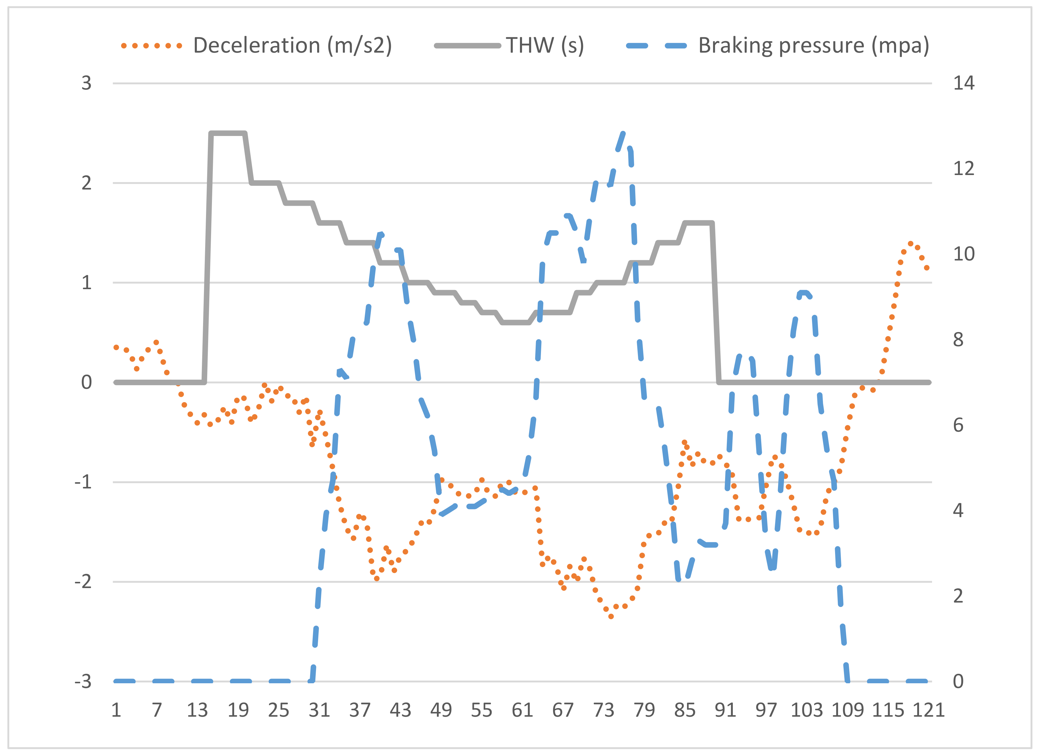
A near-crash event is an event that reached at least one of the three thresholds of indicators mentioned above. In this study the threshold values are less than 0.6 s and −0.4 m/s2 for time headway and deceleration, respectively, and more than 10 mpa for braking pressure. These thresholds are reasonable and validated by many experiments conducted in related studies, especially in China [18,20].
Figure 1 shows an example of a near-crash event observed during the naturalist driving experiment.
Before the 31-ms time-stamp, which is considered to be the starting point of a near-crash event, time headway and deceleration decreases gradually until they reached the predefined threshold values: 0.6 s and −0.4 m/s2. Braking pressure increased gradually and reached the corresponding threshold value of 10 mpa.
3. Experiment Description and Data Preparation
To present a good foundation for assessing the driving risk of near-crashes, two elements are essential to this study: driving data and experimental design. This section explains the experimental design and the data preparation. In the experimental description, the equipment, participants, and scenarios are detailed, while the data collection and preprocessing of the near-crash events are detailed in the data preparation description.
3.1. Experimental Description
3.1.1. Experimental Design
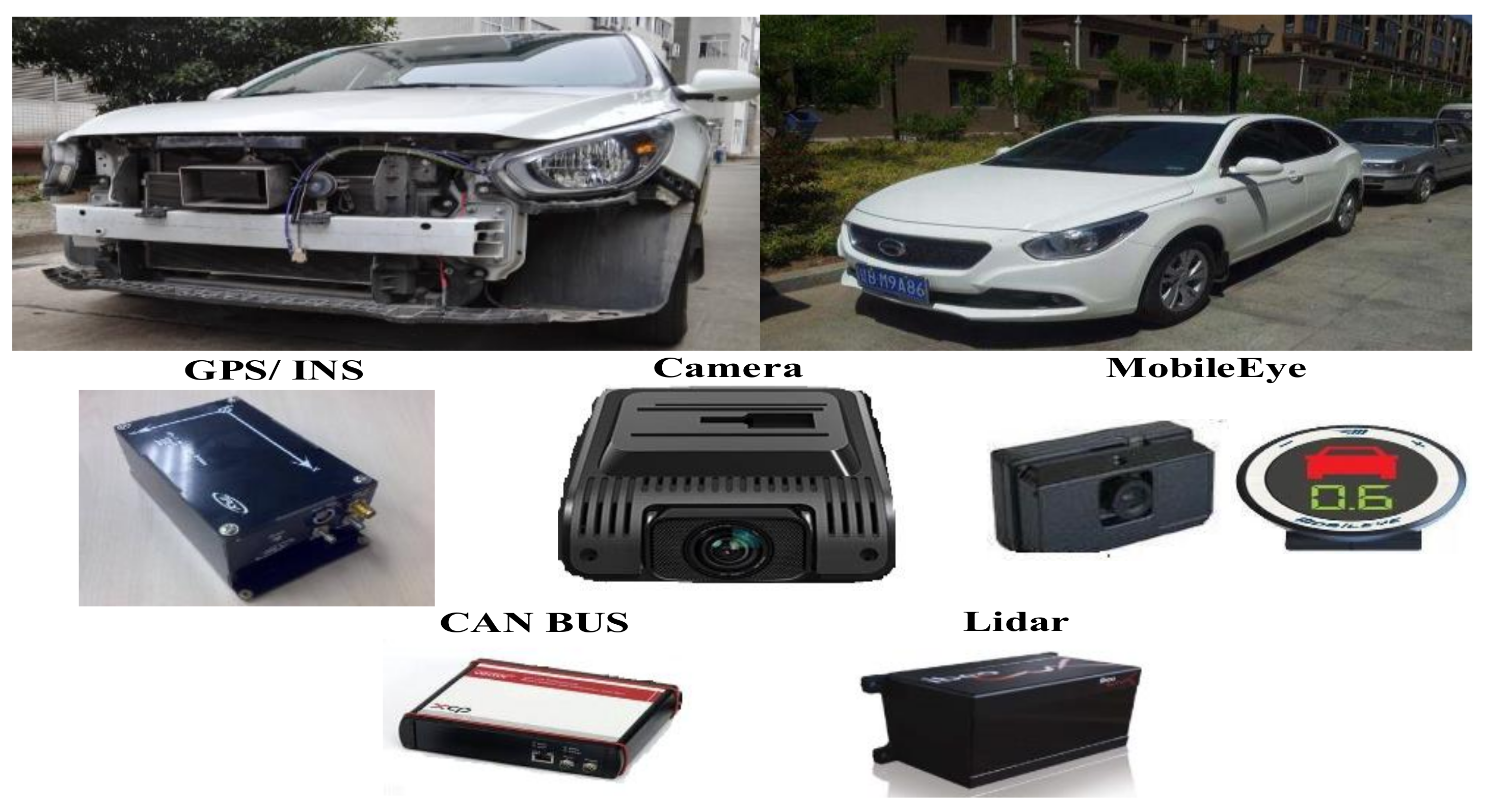
To collect near-crash data from naturalistic driving, experiments were undertaken using an instrumented vehicle on different road types in the city of Wuhan. During the experiments, each participant was informed to maintain his or her regular driving style as much as possible. In addition, to ensure that the experiments were standardized and conducted in similar conditions, the participants were asked to drive on the same routes using the same instrumented vehicle during the same periods. Experiments were conducted in September, October, and December 2016. Figure 2 shows the view from the test vehicle and its equipment and surroundings during the naturalistic driving experiment.
3.1.2. Experiment Vehicle and Equipment
The experiments were conducted using the Trump chi GA3 vehicle model manufactured by the Trump chi vehicle company. The vehicle was outfitted with different equipment to collect comprehensive data related to driving behavior and the environmental conditions. The vehicle equipment is shown in Figure 3.
A GPS/INS was used to obtain the latitude and longitude of the vehicle along with the three-axis acceleration. Time headway, lane position, and lane departure were recorded by the MobilEye device. A video camera was used to obtain environmental information during the experiments. The data for the driving behavior variables (including speed, accelerator pedal, brake pedal, and steering wheel angle) were collected by a CAN BUS. A LiDAR device was used to collect the target (vehicle) information (such as distance, velocity, relative velocity, etc.).
During the experiments, the devices collected data through the CAN bus. The experimenters used a CAN acquisition device to collect all equipment data. The clock of the collection device was set as the system clock, so all the equipment time was collected synchronously.
3.1.3. Participants
Forty-one people participated in the experiments: thirty male drivers and eleven female drivers. The drivers were recruited to participate in the experiments through a notice posted at the Wuhan University of Technology. To ensure the reliability of the experiments, the participants selected for the experiments were students and university staff, and all of them had a valid driving license (and driving experience of at least three years). The age of the participants ranged from 22 to 54 years old (the mean age was 31.85). For more details, see Table 1.
3.1.4. Experiment Routes
Because different road types have a distinct influence on driving behaviors, the experiments were conducted on different road types, including urban roads, highways, urban expressways, etc., in the city of Wuhan. In general, the urban roads consisted of two or three lanes in two directions, on which the speed limit was between 40 and 60 km/h. The total distance of the urban roads was about 12 km. The total distance of the expressways was 34 km. Each expressway consisted of three to five lanes in both directions, on which the speed limit was 80 km/h. The freeways consisted of three or four lanes in both directions, on which the speed limit was 100–120 km/h, and the total freeway distance was 45 km. Route guidance was provided to the participants by a navigation map application in the vehicle during the experiment.
3.1.5. Experimental Scenarios
Each experiment included two parts: the pre-experiment and the main experiment. In the pre-experiment, the basic courses of the experiments were explained to the participants, and then they were informed to modify the rearview mirror and the seat to be comfortable and ready to undertake the experiments. In the main experiment, each participant drove the instrumented vehicle on the predefined different types of roads, which included 45 km of freeways (40 min), 50 km of expressways (50 min), and 12 km of urban roads (36 min). Each experiment was undertaken at different times of day between 18:00 and 24:00.
3.2. Data Preparation
Using the definition of near-crashes introduced above, 1670 near-crashes were observed during the naturalistic driving experiments. The distribution of the obtained near-crashes on different road types is shown in Table 2.
As shown in Table 2, the majority of crash events occurred on urban roads followed by city highways.
To examine the factors associated with a high risk of near-crashes, this study followed approaches from previous studies for collecting and obtaining driving data variables [13,14,15]. This study introduces a comprehensive database, which includes the majority of factors that may influence the risk of near-crashes. This database contains driving behaviors, near-crash factors, environment, time, demographics, and experience.
To guarantee the quality and the accuracy of the near-crash database, the collected data needed to be filtered. After filtering for the predefined threshold of the three indicators mentioned above, the initial number of near-crash events was 1934. Then, we filtered again according to a criterion: the video of each near-crash event was watched and analyzed according to the event time. If the event was considered a near-crash (the vehicle was about to be in a crash), then this event would be saved in the database. Otherwise, the event would be excluded and removed from the database. More than five people participated in the filtering process. After filtering, the near-crash database was ready for processing using clustering and statistical models. The factors included in the near-crash database are shown in Table 3.
4. Methodology
4.1. Identification of Driving Risk of Near-Crash Events
To study the driving risk of near-crashes, it is necessary to provide a method for identifying the driving risk of near-crash events. To fill this need, a driving risk level for a near-crash event was determined by three indicators of driving behavior: minimum time headway, minimum deceleration, and maximum braking pressure, written as follows:
where represent the minimum deceleration, minimum time headway, and maximum braking pressure, respectively.
Clustering analysis is a valid approach for classifying near-crash events into different levels [24,25]. In this study, the K-means clustering method, which is used widely for cluster analysis in data-mining, was used to classify the near-crash events into different groups based on the predefined indicators. Using a predetermined number of clusters, the K-means clustering method partitions near-crash events into K clusters, where each near-crash event belongs to a cluster whose mean is closer to its value. The K-means method minimizes the within-cluster sum of squares:
where Z = [Z1, Z2, Z3, …, Zn] is a set of the obtained data, which denotes the feature in this study; S = [S1, S2, …, Si, …, Sn] is the set of the K clusters and i is the mean center of the cluster set Si. Then, the predefined K value for the K means method was set to three as in [10]. Therefore, the cluster analysis resulted in grouping the near-crash events into three driving risk groups (levels): high, moderate, and low. After that, a mixed-ordered logit model was used on the derived driving risk groups to assess the driving risk of near-crash events.
4.2. A Mixed-Ordered Logit Model for Driving Risk Levels of Near-Crash Events
The goal of this study was to evaluate the driving risk of near-crashes by exploring the contributing factors of near-crashes and considering the effect of the ordinal nature of the outcome variables.
Before performing any processes on the statistical model, there was a need to check the collinearity among the variables.
One of the methods to eliminate collinearity is to use Principal Component Analysis (PCA), as described in [26]. PCA has been successful in identifying the primary components of driver distraction to visual-manual tasks from driver performance variables. However, in our case, PCA may not be a good option as there are two types of variables (continuous and categorical), and we follow the method provided by Sunghee Park et al. [27] and Chang et al. [18]. PCA is suitable for continuous variables, such as speed and deceleration, but there are several significant categorical variables (road type and near-crash causes) in this study, and they could not be included if we used PCA. Therefore, we used Stata software, in which all variables with collinearity were identified and removed, and the results in this study have no collinearity at all.
The multiple ordinal levels for the driving risk of near-crashes (i.e., j = “1, 2, and 3”, where 1 is low, 2 is moderate, and 3 is high), which were obtained from the cluster analysis discussed in Section 4.1, facilitated the application of the ordered logit model as shown in Formula (3) [26]:
where is a latent driving risk level for a near-crash event (i = 1, 2, …, n); Xij is a matrix of explanatory variables (i.e., Xi1, Xi2, …, Xim) that affect a near-crash event I; β is the corresponding matrix of the coefficients of the regression to be estimated (i.e., β1, β2, …, βp); and denotes the term of random error, which must be independently and identically standard for logistic distribution.
To understand the severity of near-crash events and provide clear knowledge for modeling the severity of near-crash events, here is a definition of the severity index:
The severity of a near-crash event is considered by obtaining a severity index (the latent driving risk level , which was mapped to the observed driving risk level yi through the threshold ), and then each near-crash event is included in one of the three severity levels as follows:
where µ1 and µ2 are the threshold values for being estimated together with β.
The severity index would be converted into a number 1, 2, or 3 to import it into the mixed-ordered logit model.
Severity index number 1 indicates high severity, which may lead to death or incapacitation. Severity index number 2 indicates moderate severity and may lead to non-incapacitating injury or possible crash. Severity index number 3 indicates low severity, which can be a light injury or maybe only property damage or even no crash at all.
We then have the following predicted probabilities [28,29]:
where F (*) is the cumulative distribution function using the following mathematical formula [30]:
However, a limitation was detected in the traditional ordered logit model in which the coefficients of regression are fixed along with the individual observations. To address this, a mixed-ordered logit model was used to consider the coefficients being randomly distributed with the potential of various emerging parameters [30] as follows:
where is the random error that follows a normal random parameter. is used whenever is significantly bigger than 0; otherwise, the parameter would be fixed along with all individuals. Then, the conditional probability of the log likelihood function in Equation (5) would be as follows:
For selecting and comparing the model, the Akaike Information Criterion was used [29]. AIC took the goodness of fit (GOF) as well, and the model complexity was found as follows:
where L is the maximum value of the likelihood function of the model, and K is the number of the estimated parameters included in the model.
5. Results Analysis
5.1. Levels of Driving Risk of Near-Crashes
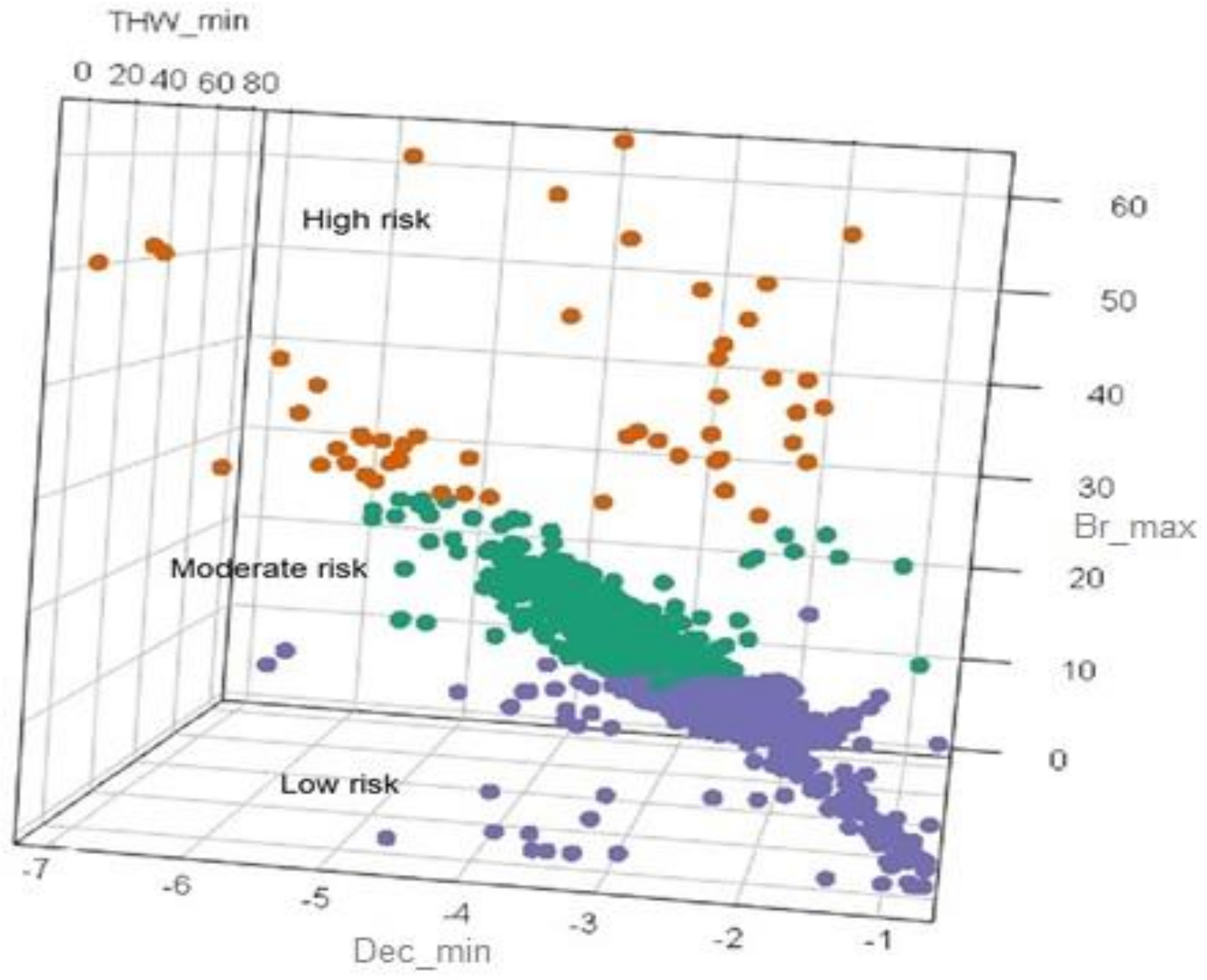
After implementing the cluster analysis, near-crash events were grouped into three levels based on their driving risk: low, moderate, or high. Figure 4 shows the clustering results and Table 4 presents the statistical details of the three risk levels.
From the data distribution of clustering the three indicators, we can use them to measure the severity of a near-crash event. In our study, cluster analysis was performed to classify the events (by the three indicators) into three clusters (risk levels): high, moderate, and low (Table 4). This is similar to the study by Wang et al. [17].
In this study, risk levels (groups) were considered as different measures for evaluating near-crash severity. For instance, in a high-risk level, the standard deviation and average maximum braking pressure were 8.44 and 41, respectively. The standard deviation and average minimum deceleration were −3.83 and 14.8, respectively. The total number of events was only 52. We can conclude that high-risk level events reflect high severity near-crash events and may lead to the high-level severity of a crash if the events become a real crash. On the other hand, in a low-risk level, the standard deviation and average maximum braking pressure were 1.8 and 1.47, respectively. The standard deviation and average minimum deceleration were −3.13 and 0.52, respectively. The total number of events was 531. We can conclude that low-risk level events reflect low severity near-crash events and may lead to the low-level severity of a crash if the events become a real crash. Table 5 summarizes the descriptive statistics of the three driving risk levels.
5.2. Results of the Statistical Model
To avoid skewed or misleading results, a correlation test was conducted to detect the existence of collinearity among the variables using Stata software as mentioned in Section 4.2. The variance inflation factor (VIF) was used, and variables with collinearity were removed. The final results indicate that the obtained maximum value of the VIF reached 3.3, and this shows that there is no strong collinearity among the independent variables in our dataset. Besides, the likelihood ratio (LR) test was used to guarantee that all added variables significantly improved the overall performance of the model.
For comparison, a mixed-ordered logit model and the original ordered logit model were used.
5.2.1. Comparison of Models
Table 6 summarizes the results of the Good of Fit (GOF) measures of the ordered logit model and the mixed-ordered logit model. Incorporating the random parameters increased the model complexity but led to a significant improvement in overall fit as denoted by LL (β). Mainly, the mixed model was superior concerning AIC statistics (15 points lower).
In addition, the adjusted log likelihood ratio index, in which higher values for a specific model indicate that this model explains the data better than the other models, of the mixed model was 0.307, which is higher than that of the basic form (0.270).
The results of the comparison show that the presence of the random parameters highlights the heterogeneity in the effects of driving risk factors of near-crashes. Therefore, this section presents explanations of the contributing factors produced by the mixed-ordered logit model.
5.2.2. Model Estimates
Table 7 shows the estimates of factors from the mixed-ordered logit model of the driving risk of near-crash events. The variables with a significance value above 0.05 or above 0.1 are highlighted. The other variables were considered insignificant and thus were eliminated from the estimated results.
In this Section, we highlight the values and signs of the estimated coefficient β. It is important to remember that a negative (or positive) value of coefficient βi is related to an increase of the corresponding variable XI, which may decrease (or increase) the probability of high driving risk and may increase (or decrease) the probability of low driving risk.
In this study, the explanatory variables that resulted in coefficients with positive signs were low deceleration average, traffic lights as a crash cause, road congestion, time of day period between 18:00 and 24:00. In other words, a near-crash event that happens on a congested road or at a traffic light location or occurs in the period 18:00–24:00 may increase the probability of being in a high driving risk. In addition, a near-crash event with a low deceleration average is more likely to increase the driving risk. As shown in Table 5, the two largest positive variables (with a coefficient value greater than 1) were associated with a time of day 18:00–24:00 followed by the deceleration average. This means that these variables are the most critical and may significantly increase the driving risk of near-crashes. By comparing the estimated coefficients of variables in Table 7, we can rank the influence of all variables on the average driving risk. We found that the variable time of day 18:00–24:00 has the greatest impact on driving risk (β = 1.140956).
In addition, the variables with negative coefficients included vehicle kinetic energy, near-crash causes, such as head vehicle suddenly stopped, road maintenance, or subject vehicle turning, road types, such as city highways and ramps, weekends, drivers older than 45, and drivers who drove fewer miles and had less driving experience. Moreover, the vehicle kinetic energy was combined with the largest negative parameter presented in Table 7, which shows that the average driving risk may decrease significantly if a near-crash has a high negative value of vehicle kinetic energy. As the vehicle kinetic energy is a driving behavior variable, it is vital to provide suitable regulations for driver behavior, which in turn enhance traffic safety.
5.2.3. Margin Effects
Interpreting the coefficients is complicated, and they cannot directly represent the magnitude of the influence of the estimates of the variables; therefore, examining the trends and patterns of the marginal effects is more insightful and intuitive [30]. Thus, Table 8 summarizes the results of the marginal effects that could be interpreted as the average percentage (%) change of the probability due to the difference in the significant factors of the three driving risk levels.
The values of the marginal effects of each variable conform to the previous findings in the estimated coefficient of high and low driving risk as discussed in Section 5.2.2.
For instance, traffic lights and road maintenance, as near-crash causes, are considered influential factors. The marginal effects of road maintenance for low and high risk were 0.4695475 and 0.0352959, respectively, whereas the marginal effects of traffic lights for low and high risk were 0.2276311 and 0.6782394, respectively. Compared with near-crashes that occur due to road maintenance, near-crashes as a result of traffic lights are more likely to cause a high-risk crash (if it happens). The impact of the other variables can also be explained in this way.
6. Discussion
Comparing this study to the study by Wang et al. [17], we highlight several similarities and dissimilarities. Regarding their methodology and results in particular, this study has several differences and innovations.
Firstly, a comprehensive experiment was conducted on different road types in the city of Wuhan in China to cover all variables associated with the driving risk of near-crashes. The obtained variables include driving behavior, near-crash factors, environment, time, demographics, and experience. In contrast, key variables were not included by Wang et al. [17], such as the maximum and average braking pressure, the average speed, average and maximum time headway, number of lanes, weekend, peak hours, time of day, and driving mileage. These variables undoubtedly play a vital role in evaluating the driving risk of near-crashes, and some of these variables were found to be significant according to the results of this study.
Secondly, unlike the definition of near-crashes proposed by Wang et al. [17], who only considered braking variables, this study presents a definition of near-crash events considering three variables: time headway, braking pressure, and deceleration. These variables provide a more powerful expression of and meaning behind driving risk of near-crashes.
Thirdly, contrary to the method used by Wang et al. [17], which was a K-means method to group near-crash events based on driving risk into three levels (high, moderate and low), this study grouped near-crash events using various variables related to driving behavior, minimum time headway, minimum deceleration, and maximum braking pressure.
Finally, Wang et al. [17] adopted a classification and tree regression model (CART) to examine contributing factors to the driving risk of near-crashes, but this study adopted a mixed-ordered logit model. The use of the CART model resulted in four significant variables: triggering factors, velocity when braking, potential object type, and possible crash type. In our study, the use of a mixed-ordered logit model resulted in more significant variables: vehicle kinetic energy, average deceleration, near-crash type, near-crash cause, road type, weekend, time of day, road congestion, driver age, driving miles, and driving experience.
Moreover, this study provides an analysis of the effect of these variables on the three levels of driving risk, which presents a better and a more comprehensive view of the impact of these variables on the driving risk of near-crashes.
The driving risk of near-crashes was identified by a clustering method (K-means) to be within one of three levels (1, high; 2, moderate; and 3, low) as in Wang et al. [17] not considering probability for specifying risk. The risk level of near-crash events was obtained using a mixed-ordered logit model to specify the factors (variables) associated with the driving risk of near-crash events. Operating the mixed-ordered logit model requires uploading the risk levels in ordinal nature (not factual numbers), and it provides the results automatically.
The significant variables influencing the driving risk of near-crashes were categorized into two types: continuous variables and categorical variables, as highlighted in Table 3 and Table 7. Ten variables were considered to be significant, including two continuous variables of driving behavior, one categorical variable of near-crash factors, four categorical variables of environment and time, and three variables (two continuous and one categorical) of driver demographics and driving experience. The negativity or positivity of the coefficient indicates the decreasing or increasing effect of the driving risk of near-crash events. A detailed description of the impact of the variables is next.
The two significant variables regarding driving behavior are vehicle kinetic energy and average deceleration. Since vehicle kinetic energy represents the upper bound and the lower bound changes of the vehicle speed, many studies have shown that the higher the value of speed, the higher the potentiality of being in a crash [31,32]. This indicates that the driving risk of a near-crash event will increase as the vehicle speed increases. The vehicle deceleration reflects the driver’s control of operating devices, such as the brake pedal and accelerator pedal. The average deceleration was considered to be an important variable in this study. Generally, if the driver performed an urgent brake, then the vehicle may have a very urgent traffic risk situation. In such an emergency, the driver will avoid a collision by a heavy brake. Many studies support this finding [33,34,35,36]. To sum up our findings, two variables—vehicle kinetic energy and average deceleration—related to driving behavior are important and conform to those found in previous studies on road safety.
Regarding the near-crash causes, four categorical factors—the head vehicle suddenly stopped, traffic lights, road maintenance, and subject vehicle turning—were found to be significant factors. Results shown in Table 7 support the statistical results shown in Table 5. Three factors of near-crash cause have significant effects on the driving risk of near-crashes. When a head vehicle suddenly stops, the possibility of being in a crash is higher as the driver of the behind vehicle may not react fast enough. Additionally, a crash may occur due to: (1) a traffic light change, which may cause a vehicle to suddenly stop; and (2) a reduction in vehicle speed due to road maintenance. These results also conform to the previous study [17].
In addition, four variables related to environment and time have a significant impact on driving risk. These variables are road type, congestion, time of day, and weekend. Regarding road type, two categorical factors, city highway and ramp, are considered to be significant factors. City highways and ramps represent two common road types where crashes may occur. These findings conform with previous studies that examined the impact of road geometries on crash risk [37,38,39]. The time of day (18:00–24:00) variable was also found to have a significant influence on driving risk in this study. The reasons for this may relate to light and visibility conditions, congestion, higher levels of tiredness, and this result conforms with a previous study [35].
Three variables of driver demographics and driving experience are significantly correlated with driving risk, namely age, driving miles, and driving experience. Regarding age, a person who is over 45 years old shows a significantly higher driving risk of near-crash events. This may be due to the reduced physical and cognitive skills of older drivers. Older drivers have a significantly growing rate of probability for committing driving errors, and this may lead to high risk and serious crashes. This conforms to the findings of a previous study [40]. In addition, this study considered driving miles and experience to be significant variables. This is reasonable as these variables provide measures of driving ability and experience. Driving experience represents the license period of a driver, whereas driving miles represent the actual miles driven by a driver. These findings conform with previous findings [40,41].
7. Conclusions
This study explored the contributing factors associated with driving risk of near-crashes using a mixed-ordered logit model. In total, 1670 near-crashes were captured in naturalistic driving experiments conducted by 41 participants on different road types in the city of Wuhan in China. The experiments found the significant variables influencing driving risk include driver behavior, near-crash factors, environment, time, demographics, and experience.
This study proposes a new definition of near-crash events by detecting one (or more than one) of the three thresholds on the following driving behavior factors: (1) the deceleration threshold is less than −0.4 m/s2; (2) the braking pressure threshold is greater than 10 mpa; and (3) the time headway threshold is less than 0.6 s.
The K-means method was used to group the near-crash events based on their driving risk using three variables: minimum deceleration, minimum time headway, and maximum braking pressure. The K-means method produced three driving risk levels (groups): low, moderate, and high. Then, a mixed-ordered logit model was used to explore the significant factors associated with the driving risk of near-crash events.
The results of using the model indicate that ten factors are significant: deceleration average, vehicle kinetic energy, near-crash causes, congestion, time of day, road type, driving miles, weekend, driver age, and experience. The findings may be used by transportation planners to understand the factors that influence the driving risk of road traffic and may provide valuable insights and helpful suggestions for improving transportation rules and reducing traffic collisions thus making roads safer.
For future work, there is a need to investigate the role of road users (such as pedestrians and motorcyclists) on driving risk. Integrating crash data of motorcycles on risky intersections in the city of Wuhan will also be studied. This can provide insights in investigating the contributing factors to driving risk. In addition, the impact of distractions, such as mobile phones, on driving risk is another aspect that will be studied in future work.
Author Contributions
H.A.H.N. developed the methodology and analyzed the data; C.W. contributed material, experimentals devices and analysis tools; N.L. conceived and designed the experiments; H.A.H.N. and N.L. performed the experiments; H.A.H.N. wrote the paper; and Q.X. and K.Z. helped in writing and editing.
Funding
This study was funded and supported by several projects: National Nature Science Foundation of China (Grant No. 51178364); National Nature Science Foundation of China (Grant No. 61603282); and Nature Science Foundation of China (Grand No. 51678460).
Acknowledgments
The authors thank all experiments participants and all students who participated in data preprocessing.
Conflicts of Interest
The authors declare no conflict of interest.
References
- National Bureau of Statistics. The People’s Republic of China Statistical Yearbook of Road Traffic Accidents 2015; National Bureau of Statistics of China: Wuxi, China, 2016.
- Li, Z.; Liu, P.; Wang, W.; Xu, C. Using support vector machine models for crash injury severity analysis. Accid. Anal. Prev. 2012, 45, 478–486. [Google Scholar] [CrossRef] [PubMed]
- Chen, C.; Zhang, G.; Qian, Z.; Tarefder, R.A.; Tian, Z. Investigating driver injury severity patterns in rollover crashes using support vector machine models. Accid. Anal. Prev. 2016, 90, 128–139. [Google Scholar] [CrossRef] [PubMed]
- Iragavarapu, V.; Lord, D.; Fitzpatrick, K. Analysis of injury severity in pedestrian crashes using classification regression trees. In Proceedings of the Transportation Research Board Annual Meeting, Washington, DC, USA, 11–15 January 2015. [Google Scholar]
- Chang, L.Y.; Chien, J.T. Analysis of driver injury severity in truck-involved accidents using a non-parametric classification tree model. Saf. Sci. 2013, 51, 17–22. [Google Scholar] [CrossRef]
- Chen, C.; Zhang, G.; Huang, H.; Wang, J.; Tarefder, R.A. Examining driver injury severity outcomes in rural non-interstate roadway crashes using a hierarchical ordered logit model. Accid. Anal. Prev. 2016, 96, 79. [Google Scholar] [CrossRef] [PubMed]
- Bogue, S.; Paleti, R.; Balan, L. A modified rank ordered logit model to analyze injury severity of occupants in multivehicle crashes. Anal. Methods Accid. Res. 2017, 14, 22–40. [Google Scholar] [CrossRef]
- Guo, F. Near-Crashes as crash surrogate for naturalistic driving studies. Transp. Res. Rec. J. Transp. Res. Board. 2010, 2147, 66–74. [Google Scholar] [CrossRef]
- Tarko, A.; Davis, G.A.; Saunier, N.; Sayed, T. Surrogate Measures of Safety. In Safe Mobility: Challenges, Methodology and Solutions; Emerald Publishing Limited: Bingley, UK, 2018; pp. 383–405. [Google Scholar]
- Zheng, Y.; Wang, J.; Li, X.; Yu, C. Driving risk assessment using cluster analysis based on naturalistic driving data. In Proceedings of the IEEE International Conference on Intelligent Transportation Systems, Qingdao, China, 8–11 October 2014; IEEE: Piscataway, NJ, USA, 2014. [Google Scholar]
- Young, R.A. Revised odds ratio estimates of secondary tasks: A re-analysis of the 100-car naturalistic driving study data. Sae Tech. Pap. 2015. [Google Scholar] [CrossRef]
- Takeda, K.; Hansen, J.H.L.; Boyraz, P.; Malta, L.; Miyajima, C.; Abut, H. International large-scale vehicle corpora for research on driver behavior on the road. IEEE Trans. Intell. Transp. Syst. 2011, 12, 1609–1623. [Google Scholar] [CrossRef]
- Wu, K.F.; Aguero-Valverde, J.; Jovanis, P.P. Using naturalistic driving data to explore the association between traffic safety-related events and crash risk at driver level. Accid. Anal. Prev. 2014, 72, 210–218. [Google Scholar] [CrossRef] [PubMed]
- Moreno, A.T.; García, A. Use of speed profile as surrogate measure: Effect of traffic calming devices on crosstown road safety performance. Accid. Anal. Prev. 2013, 61, 23–32. [Google Scholar] [CrossRef] [PubMed] [Green Version]
- Wu, K.F.; Jovanis, P.P. Screening naturalistic driving study data for safety-critical events. Transp. Res. Rec. J. Transp. Res. Board 2013, 2386, 137–146. [Google Scholar] [CrossRef]
- Guo, F.; Fang, Y. Individual driver risk assessment using naturalistic driving data. Accid. Anal. Prev. 2013, 61, 3–9. [Google Scholar] [CrossRef] [PubMed]
- Wang, J.; Zheng, Y.; Li, X.; Yu, C.; Kodaka, K.; Li, K. Driving risk assessment using near-crash database through data mining of tree-based model. Accid. Anal. Prev. 2015, 84, 54–64. [Google Scholar] [CrossRef] [PubMed]
- Chang, F.; Li, M.; Xu, P.; Zhou, H.; Haque, M.M.; Huang, H. Injury severity of motorcycle riders involved in traffic crashes in Hunan, China: A mixed ordered logit approach. Int. J. Environ. Res. Public Health. 2016, 13, 714. [Google Scholar] [CrossRef] [PubMed]
- Lyu, N.; Deng, C.; Xie, L.; Wu, C.; Duan, Z. A field operational test in China: Exploring the effect of an advanced driver assistance system on driving performance and braking behavior. Transp. Res. Part F Traff. Psychol. Behav. 2018. [Google Scholar] [CrossRef]
- Lyu, N.; Ren, Z.; Duan, Z.; Luo, Y. Analysis of driving behavior characteristics of drivers in Near-crash events. China Saf. Sci. J. 2017, 27, 19–24. (In Chinese) [Google Scholar]
- Lu, G.; Cheng, B.; Lin, Q.; Wang, Y. Quantitative indicator of homeostatic risk perception in car following. Saf. Sci. 2012, 50, 1898–1905. [Google Scholar] [CrossRef]
- Bagdadi, O. Assessing safety critical braking events in naturalistic driving studies. Transp. Res. Part F Traffic Psychol. Behav. 2013, 16, 117–126. [Google Scholar] [CrossRef]
- Tarko, A.; Davis, G.; Saunier, N.; Sayed, T.; Washington, S. White Paper: Surrogate Measures of Safety; Transportation Research Board, National Research Council: Washington, DC, USA, 2009. [Google Scholar]
- Shewhart, W.A.; Wilks, S.S. Cluster Analysis, 5th ed.; Elsevier: New York, NY, USA, 2011. [Google Scholar]
- Witten, I.H.; Frank, E.; Hall, M.A. Data Mining: Practical Machine Learning Tools and Techniques; Morgan Kaufmann: Burlington, MA, USA, 2011; pp. 76–77. [Google Scholar]
- Young, R.; Seaman, S.; Li, H. The dimensional model of driver demand: Visual-manual tasks. Sae Int. J. Transp. Saf. 2016, 4, 33–71. [Google Scholar] [CrossRef]
- Park, S.; Jang, K.; Park, S.H.; Kim, D.K.; Chon, K.S. Analysis of injury severity in traffic crashes: A case study of korean expressways. KSCE J. Civ. Eng. 2012, 16, 1280–1288. [Google Scholar] [CrossRef]
- Faraway, J.J. Linear Models with R, 2nd ed.; Crc Press: Boca Raton, FL, USA, 2014. [Google Scholar]
- Liu, X.; Koirala, H. Ordinal regression analysis: Using generalized ordinal logistic regression models to estimate educational data. J. Mod. Appl. Stat. Methods JMASM 2012, 11, 242–254. [Google Scholar] [CrossRef]
- Heiss, F. Discrete Choice Methods with Simulation; Cambridge University Press: Cambridge, UK, 2003; pp. 688–692. [Google Scholar]
- Wu, C.; Sun, C.; Chu, D.; Huang, Z.; Ma, J.; Li, H. Clustering of several typical behavioral characteristics of commercial vehicle drivers based on gps data mining. Transp. Res. Rec. J. Transp. Res. Board 2016, 2581, 154–163. [Google Scholar] [CrossRef]
- Miyajima, C.; Ukai, H.; Naito, A.; Amata, H.; Kitaoka, N.; Takeda, K. Driver risk evaluation based on acceleration, deceleration, and steering behavior. In Proceedings of the IEEE International Conference on Acoustics, Speech and Signal Processing, Prague, Czech Republic, 22–27 May 2011; IEEE: Piscataway, NJ, USA, 2011. [Google Scholar]
- Tak, S.; Kim, S.; Yeo, H. Development of a deceleration-based surrogate safety measure for rear-end collision risk. IEEE Trans. Intell. Transp. Syst. 2015, 16, 2435–2445. [Google Scholar] [CrossRef]
- Rakha, H.; El-Shawarby, I.; Setti, J.R. Characterizing driver behavior on signalized intersection approaches at the onset of a yellow-phase trigger. IEEE Trans. Intell. Transp. Syst. 2007, 8, 630–640. [Google Scholar] [CrossRef]
- Qu, X.; Yang, Y.; Liu, Z.; Jin, S.; Weng, J. Potential crash risks of expressway on-ramps and off-ramps: A case study in Beijing, China. Saf. Sci. 2014, 70, 58–62. [Google Scholar] [CrossRef]
- Qu, X.; Meng, Q. A note on hotspot identification for urban expressways. Saf. Sci. 2014, 66, 87–91. [Google Scholar] [CrossRef]
- Ward, H.; Shepherd, N.; Robertson, S.; Thomas, M. Night-Time Accidents: A Scoping Study; Report to The AA Motoring Trust and Rees Jeffreys Road Fund; UCL (University College London): London, UK, 2005. [Google Scholar]
- Guo, F.; Klauer, S.G.; Fang, Y.; Hankey, J.M.; Antin, J.F.; Perez, M. The effects of age on crash risk associated with driver distraction. Int. J. Epidemiol. 2017, 46, 258–265. [Google Scholar] [CrossRef] [PubMed]
- Ko, M.; Park, B.J.; Wu, L.; Walden, T.D. Exploring the relationship between driver errors and age in vehicle crash data. In Proceedings of the Transportation Research Board Annual Meeting, Washington, DC, USA, 11–15 January 2015. [Google Scholar]
- Curry, A.; Pfeiffer, M.; Durbin, D.; Elliott, M.; Kim, K. Young driver crash rates in new jersey by driving experience, age, and license phase. Driver Exp. 2014, 80, 245–250. [Google Scholar]
- Curry, A.E.; Pfeiffer, M.R.; Durbin, D.R.; Elliott, M.R. Young driver crash rates by licensing age, driving experience, and license phase. Accid. Anal. Prev. 2015, 80, 243–250. [Google Scholar] [CrossRef] [PubMed]
Figure 1.
An example of a near-crash event.

Figure 2.
A photograph of the experimental vehicle, equipment, and surroundings.

Figure 3.
Experimental vehicle and equipment.

Figure 4.
Results of the cluster analysis of driving risk for near-crash events.


Table 1.
Participant information.
| Total | Age (by Years) | Experience (by Years) | Driving Miles | ||||
|---|---|---|---|---|---|---|---|
| Mean | SD | Mean | SD | Mean | SD | ||
| All | 41 | 31.85 | 8.23 | 6.7 | 4.49 | 266.44 | 13.4 |
| Male | 30 | 31.46 | 8.11 | 6.2 | 4.37 | 302.90 | 10.9 |
| Female | 11 | 33.00 | 8.74 | 8 | 4.83 | 158.90 | 17.2 |
Table 2.
Near-crash events on different road types.
| Urban Roads | City Highways | Freeways | Ramps | Tunnels | |
|---|---|---|---|---|---|
| Near-Crash Events | 694 | 515 | 228 | 191 | 42 |
Table 3.
Factors of the near-crash database.
| Factor | Symbol | Data-Type | Source | Description |
|---|---|---|---|---|
| Driving Behavior | ||||
| Starting Speed | Be_Sp | continuous | Signals | Speed when a near-crash event begins (m/s) |
| Deceleration Average | Avr_Dec | continuous | Signals | Average Deceleration (m/s2) |
| Average Speed | Avr_Sped | continuous | Signals | Average Speed (m/s) |
| Time Headway Average | Avr_THW | continuous | Signals | Average Time Headway (s) |
| Braking pressure Average | Avr_Br | continuous | Signals | Average Braking Pressure (MPA) |
| Min Deceleration | Min_Dec | continuous | Signals | Minimum Deceleration (m/s2) |
| Min Time Headway | MinTHW | continuous | Signals | Minimum Time Headway (s) |
| Max Braking pressure | Max_Br | continuous | Signals | Maximum Braking Pressure (MPA) |
| Energy * | Energy | continuous | Signals | Vehicle Kinetic Energy |
| Near-Crash Factors | ||||
| Near-Crash Type | Cra_ty | categorical | Video | Potential Crash Type 1. Subject (head)-object (head) 2. Subject (head)-object (tail) 3. Subject (head)-object (side) 4. Subject (side)-object (side) 5. Subject (side)-object (tail) 6. Pedestrian conflict 7. Road parts 8. Others |
| Near-Crash Reason | NC_reasn | categorical | Video | Near-crash Cause 1. Head vehicle suddenly stopped 2. Traffic lights 3. Traffic density 4. Road maintenance 5. Road changes 6. Road users 7. Subject vehicle turning 8. Object vehicle turning 9. Others |
| Environment and Time Features | ||||
| Wet | Wet | categorical | Video | Road condition 1. Wet 2. Dry |
| Road Type | R_ty | categorical | Video | Road Types 1. Urban roads 2. City Highways 3. Freeways 4. Ramp 5. Tunnel |
| Lane Numbers | Lane_Nu | categorical | Video | Lane numbers 1.1, 2.2, 3.3, 4.4, 5.5 |
| Speed Limit | Sp_lim | categorical | Video | Speed limit 1. 60 2. 80 3. 100–120 |
| Road Congestion | congested | categorical | Video | Is congested? 1. Yes; 0. No |
| Peak Hour | Peak_hrs | categorical | Video | Is it in peak hours (7:30–9:00 am, 4:30–5:30 pm) 1. Yes; 2. No |
| Weather | Weather | categorical | Video | Weather 1. Sunny 2. Rain 3. Cloud |
| Light | Light | categorical | Video | Light 1. Light 2. Dark |
| Weekend | Weekend | categorical | Signals | Weekend 1. Yes 2. No |
| Time of Day | Time_day | categorical | Signals | Time of day 1. 06–12 2. 12–18 3. 18–24 |
| Driver and Driving Experience Factors | ||||
| Age | Age | categorical | Questionnaire | Age 1. Less than 23 2. 23–45 3. More than 45 |
| Gender | Gender | categorical | Questionnaire | Gender 1. Male 2. Female |
| Driving Miles | Driving_miles | continuous | Questionnaire | Driving Miles (miles) |
| Driving Experience | Dri_years | continuous | Questionnaire | Driving years with license (years) |
Energy * (Vehicle Kinetic Energy) was calculated by the formula: , where v1 and v2 represent the highest and lowest speed during a near-crash event.
Table 4.
Characteristics of driving risk levels.
| Driving Risk Levels | Events Number | Percentile (%) | Mean and SD of Driving Behavior Characteristics | |||||
|---|---|---|---|---|---|---|---|---|
| THW_Min (m/s) | DEC_Min (m/s2) | Br_Max (MPA) | ||||||
| Mean | SD | Mean | SD | Mean | SD | |||
| Low | 531 | 31.8 | 1.80 | 1.47 | −3.13 | 0.52 | 21.28 | 3.12 |
| Moderate | 1087 | 65 | 2.32 | 3.64 | −2.15 | 0.51 | 13.19 | 3.27 |
| High | 52 | 3.2 | 2.05 | 0.87 | −3.83 | 1.48 | 41.00 | 8.46 |
Table 5.
Summary of descriptive statistics of factors.
| Factor | Events No | Low | Moderate | High | Factor | Events No | Low | Moderate | High |
|---|---|---|---|---|---|---|---|---|---|
| % | % | % | % | % | % | ||||
| Crash Type | Lane Numbers | ||||||||
| 1. Subject (head)-object (head) | 14 | 28.5 | 71.5 | 0 | 1. One Lane | 91 | 30.6 | 65.1 | 4.3 |
| 2. Subject (head)-object (tail) | 1053 | 31.7 | 65.9 | 2.3 | 2. Two Lanes | 366 | 34 | 63.3 | 2.7 |
| 3. Subject (head)-object (side) | 306 | 33.3 | 64.7 | 1.9 | 3.Three Lanes | 780 | 30 | 67.1 | 3.3 |
| 4. Subject (side)-object (side) | 30 | 23.3 | 70 | 6.6 | 4. Four Lanes | 427 | 33.4 | 62.7 | 4.6 |
| 5. Subject (side)-object (tail) | 12 | 16.6 | 83.3 | 0 | 5. Five Lanes | 14 | 28.5 | 42.85 | 14.2 |
| 6. Pedestrian conflict | 28 | 35.7 | 64.2 | 0 | Time of Day | ||||
| 7. Road parts | 59 | 35.5 | 61.0 | 3.3 | 1.06–12 | 743 | 32.8 | 64.7 | 2.4 |
| 8. Others | 168 | 30.3 | 59.5 | 10.1 | 2.12–18 | 888 | 30.9 | 65.4 | 3.6 |
| Near-Crash Reason | 3.18–24 | 39 | 30.7 | 64.1 | 5.1 | ||||
| 1. Head Vehicle Suddenly Stopped | 247 | 31.5 | 66.3 | 2.0 | Road Congestion | ||||
| 2. Traffic Lights | 153 | 24.8 | 67.3 | 7.8 | 0. No | 883 | 34.8 | 62.9 | 2.1 |
| 3. Traffic Density | 600 | 35.6 | 6.2 | 2.3 | 1. Yes | 787 | 28.3 | 67.4 | 4.1 |
| 4. Fixing Road | 14 | 42.8 | 57.1 | 0 | Peak Hour | ||||
| 5. Road Changes | 59 | 27.1 | 71.1 | 1.6 | 1. Yes | 370 | 30.8 | 67.2 | 1.9 |
| 6. Road Users | 32 | 37.5 | 62.5 | 0 | 2. No | 1300 | 32 | 64.4 | 3.4 |
| 7. Subject Vehicle Turning | 182 | 31.3 | 67.5 | 1.0 | Weather | ||||
| 8. Object Vehicle Turning | 222 | 28.8 | 68.9 | 2.2 | 1. Sunny | 1499 | 32.1 | 65.3 | 2.5 |
| 9. Others | 161 | 28.5 | 63.3 | 8.0 | 2. Rain | 98 | 31.6 | 653 | 3 |
| Road Type | 3. Cloudy | 73 | 24.6 | 60.2 | 15.2 | ||||
| 1. Urban | 694 | 30.2 | 67.2 | 2.5 | Weekend | ||||
| 2. City Highway | 515 | 33.7 | 63.8 | 2.3 | 0. Yes | 429 | 32.4 | 65.9 | 1.6 |
| 3. Freeway | 228 | 28.5 | 64 | 7.4 | 1. No | 1241 | 31.5 | 64.7 | 3.6 |
| 4. Ramp | 191 | 36.7 | 61.8 | 1.6 | Age | ||||
| 5. Tunnel | 42 | 28.6 | 66.7 | 4.7 | 1. less than 23 | 176 | 34.6 | 61.9 | 3.4 |
| Wet | 2. 23–45 | 1200 | 31.4 | 65.3 | 3.2 | ||||
| 1. Dry | 1479 | 32.1 | 65.1 | 2.7 | 3. More than 45 | 172 | 26.7 | 71.5 | 1.7 |
| 2. Wet | 194 | 28.4 | 65.6 | 6.3 | Gender | ||||
| 1. Male | 1165 | 33 | 64.6 | 2.4 | |||||
| 2. Female | 505 | 28.9 | 66.1 | 4.9 | |||||
Table 6.
Goodness-of-fit measures for the ordered logit model (basic) and the mixed-ordered logit model.
Table 6.
Goodness-of-fit measures for the ordered logit model (basic) and the mixed-ordered logit model.
| Model Statistic | Basic | Mixed |
|---|---|---|
| Observations, n | 1670 | 1670 |
| Significant parameters, k | 9 | 10 |
| Log likelihood at zero, LL (0) | −1255.5942 | −1255.5942 |
| Log likelihood at convergence, LL (β) | −911.19892 | −777.880 |
| AIC | 1639.761 | 1625.054 |
| Adj Likelihood ratio index | 0.207 | 0.307 |
| Degree of Freedom | 14 | 14 |
Table 7.
Estimate results for the mixed-ordered logit model.
| Dependent Variable | Coefficient | Standard Error | p > |z| | Z-Statistic | Mean |
|---|---|---|---|---|---|
| Driving Behavior Features | |||||
| Vehicle Kinetic Energy | −4.357163 | 0.2454721 | <0.001 * | −17.75 | 0.40211 |
| Deceleration Average | 1.102912 | 0.0846138 | <0.001 * | 13.03 | −2.042 |
| Near-Crash Features | |||||
| Near-Crash Reason | 4.42814 | ||||
| 1. Head Vehicle Suddenly Stopped | −0.4246619 | −0.2144163 | 0.048 * | −1.98 | |
| 2. Traffic Lights | 0.543326 | 0.2551985 | 0.033 * | 2.13 | |
| 3. Traffic Density a | 0 | 0 | 0 | ||
| 4. Road Fixing | −1.421049 | −0.6403748 | 0.026 * | −2.22 | |
| 7. Subject Vehicle Turning | −0.4656817 | 0.2249775 | 0.038 * | −2.07 | |
| Environment and Time | |||||
| Road Type | |||||
| 1. Urban a | 0 | 0 | 0 | 3.07964 | |
| 2. City Highway | −0.6653231 | 0.1554658 | 0.008 * | −4.28 | |
| 4. Ramp | −0.6350275 | 0.2075957 | 0.002 * | −3.06 | |
| Road Congestion | 0.52874 | ||||
| 0. Yes | 0.2926946 | 0.1613912 | 0.094 ** | 1.98 | |
| 1. No a | 0 | 0 | 0 | ||
| Time of Day | 1.57844 | ||||
| 2.12–18 a | 0 | 0 | 0 | ||
| 3.18–24 | 1.140956 | 0.4467025 | 0.011 * | 2.55 | |
| Weekend | 1.74311 | ||||
| 0. No a | 0 | 0 | 0 | 0 | |
| 1. Yes | −0.740657 | 0.3487634 | 0.081 ** | −2.16 | |
| Driver Demographic and Driving Experience Features | |||||
| Age | 1.99761 | ||||
| 2. 23–45 a | 0 | 0 | 0 | ||
| 3. More than 45 | −0.3049686 | 0.2429392 | −0.084 ** | 2.35 | |
| Driving Mileages | −0.002227 | 0.0007862 | 0.005 * | −2.83 | 89948.7 |
| Driving Experience (years) | −0.0601705 | 0.0228715 | 0.009 * | −2.63 | 6.6 |
| Threshold | Coefficient | Standard Error | |||
| Cut-point 1 (between low ~moderate) | −5.727851 | 0.3434905 | |||
| Cut-point 2 (between moderate ~high) | −5.524819 | 0.3411096 | |||
* Significant at 5%; ** Significant at 10%; a Base reference of associated categorical variable.
Table 8.
Estimate results of marginal effects of driving risk factors.
| Dependent Variable | Marginal Effects of Risk Levels | ||
|---|---|---|---|
| Low | Moderate | High | |
| Driving Behavior Features | |||
| Vehicle Kinetic Energy | 0.6876918 | −0.7180673 | 0.0303755 |
| Deceleration Average | −0.1825126 | −0.0080616 | 0.1905742 |
| Near-Crash Features | |||
| Near-Crash Reason | |||
| 1. Head Vehicle Suddenly Stopped | 0.3610219 | 0.7430515 | −0.0328883 |
| 2. Traffic Lights | 0.2276311 | 0.0263799 | 0.6782394 |
| 3. Traffic Density a | 0 | 0 | 0 |
| 4. Road Fixing | 0.4695475 | 0.4951566 | 0.0352959 |
| 7. Subject Vehicle Turning | 0.0101273 | −0.0105746 | 0.0004473 |
| Environment and Time | |||
| Road Type | |||
| 1. Urban a | 0 | 0 | 0 |
| 2. City Highway | 0.3484643 | 0.6184576 | 0.0330782 |
| 4. Ramp | 0.3480709 | 0.0330646 | 0.6188645 |
| Road Congestion | |||
| 0. Yes | 0.3254279 | 0.6422137 | 0.0323583 |
| 1. No a | 0 | 0 | 0 |
| Time of Day | |||
| 2.12–18 a | 0 | 0 | 0 |
| 3.18–24 | 0.1775779 | 0.0233632 | 0.7990589 |
| Weekend | |||
| 0. No a | 0 | 0 | 0 |
| 1. Yes | 0.3311193 | 0.6691787 | 0.032426 |
| Driver Demographic and Driving Experience Features | |||
| Age | |||
| 2. 23–45 a | 0 | 0 | 0 |
| 3. More than 45 | 0.0327717 | 0.6128834 | 0.354345 |
| Driving Mileages | −4.10 × 10⁻⁷ | 4.28 × 10⁻⁷ | −1.81 × 10⁻⁸ |
| Driving Experience (years) | 0.0093566 | −0.0097702 | 0.0004135 |
a Base reference of associated categorical variable.
© 2018 by the authors. Licensee MDPI, Basel, Switzerland. This article is an open access article distributed under the terms and conditions of the Creative Commons Attribution (CC BY) license (http://creativecommons.org/licenses/by/4.0/).
Share and Cite
MDPI and ACS Style
Naji, H.A.H.; Xue, Q.; Lyu, N.; Wu, C.; Zheng, K. Evaluating the Driving Risk of Near-Crash Events Using a Mixed-Ordered Logit Model. Sustainability 2018, 10, 2868. https://0-doi-org.brum.beds.ac.uk/10.3390/su10082868
AMA Style
Naji HAH, Xue Q, Lyu N, Wu C, Zheng K. Evaluating the Driving Risk of Near-Crash Events Using a Mixed-Ordered Logit Model. Sustainability. 2018; 10(8):2868. https://0-doi-org.brum.beds.ac.uk/10.3390/su10082868
Chicago/Turabian StyleNaji, Hasan. A. H., Qingji Xue, Nengchao Lyu, Chaozhong Wu, and Ke Zheng. 2018. "Evaluating the Driving Risk of Near-Crash Events Using a Mixed-Ordered Logit Model" Sustainability 10, no. 8: 2868. https://0-doi-org.brum.beds.ac.uk/10.3390/su10082868
Note that from the first issue of 2016, this journal uses article numbers instead of page numbers. See further details here.