Managing Procurement for a Firm with Two Ordering Opportunities under Supply Disruption Risk


Business School, Nankai University, Tianjin 300071, China
*
Author to whom correspondence should be addressed.
Sustainability 2018, 10(9), 3293; https://0-doi-org.brum.beds.ac.uk/10.3390/su10093293
Submission received: 17 July 2018
/
Revised: 27 August 2018
/
Accepted: 12 September 2018
/
Published: 14 September 2018
(This article belongs to the Special Issue Sustainable Supply Chain System Design and Optimization)
Abstract
:Supply disruption is a common phenomenon in industry, which brings destructive effects to downstream firms and damages the sustainability of the supply chain. To mitigate the supply disruption risk, the authors investigate two types of procurement strategies for a firm with two ordering opportunities. Through establishing Stackelberg game models, the authors drive the supplier’s optimal production, and the firm’s optimal procurement and replenishment strategies under the option purchase (OP) strategy and the procurement commitment (PC) strategy, respectively. The findings show that, under both types of strategies, the firm’s procurement follows a “threshold” principle. Moreover, the firm’s procurement quantity can be represented by two newsvendor solutions. A lower option price or option exercise price benefits the firm, while it damages the supplier. The supplier benefits from a higher mean value (MV) of emergency procurement price and the firm benefits from a lower market demand variability. Counter-intuitively, a lower MV of the emergency procurement price is not always beneficial to the firm. A higher market demand variability could be beneficial to the supplier under the PC strategy. The firm should first choose the PC strategy and then change to the OP strategy as the disruption risk increases.
1. Introduction
The recent trade disputes between the US and China and the increasing frequency of natural and anthropogenic catastrophes indicate the need for organizations to hedge their supply chains against major disruptions [1,2]. Supply chain disruption might result in severe problems in many aspects, such as enterprise bankruptcy, job losses, stock market crash, panic buying, and more. All of these not only damage the reputation of the related firm and the interests of shareholders, but also lead to social instability, which affects the sustainability of the supply chain [3,4]. The recent U.S. ban on exports of Chinese telecommunications equipment and smartphone maker ZTE, which employs roughly 75,000 workers and had been worth about $20 billion before the ban, immediately put the company out of business and in a state of shock (https://www.scmp.com/tech/article/2142557/zte-calls-us-government-ban-extremely-unfair-vows-fight-its-rights, accessed date 20 June 2018), for example. The Great East Japan Earthquake in March 2011, and the subsequent Fukushima nuclear accident, impacted some highly concentrated industrial facilities on which many industries worldwide depended, so numerous supply chains across many industries were disrupted [5]. A large number of firms, including those in other countries such as the US, South Korea, Thailand, and France, had to cease operations due to shortage of supply (https://www.rieti.go.jp/en/columns/v01_0085.html, 25 April 2017).
To manage the supply disruption risk and maintain the sustainability of the supply chain, many strategies have been proposed, such as multi-sourcing, emergency sourcing/production, holding inventory, and supplier process improvement [6,7,8,9,10,11,12]. The authors investigate two types of procurement strategies, namely, the option purchase (OP) strategy and the procurement commitment (PC) strategy, for a firm with two ordering opportunities to mitigate the supply disruption risk. This study is motivated by the procurement risk management practice at Hewlett-Packard (HP) company [13,14]. To manage the uncertainties in product demand, component price, and component availability, HP adopted a combination of traditional long-term contracts and more flexible short-term contracts. The PC strategy and OP strategy used in this paper, in fact, belong to the traditional long-term contract and flexible short-term contract, respectively. Under the PC strategy, the firm can buy a fixed quantity at a relatively low and fixed price before the demand is realized. Using the OP strategy, the firm can reserve a pre-determined amount of stock beforehand and adjust its ordering quantity at selling season. Additionally, the authors also consider the situation where the firm has two ordering opportunities. That is to say, the firm can order from the supplier before and after the demand is realized, respectively. Actually, adopting two or more ordering opportunities is a common phenomenon for a firm [15]. Regarding the case of HP, for example, it could procure from its suppliers in advance or postpone its procurement after the demand uncertainty is resolved [13,14]. International Business Machines Corporation (IBM) and Oracle also use such a flexible approach to purchasing [16].
Supply disruption usually brings about an increase and uncertainty in price. The devastating shortage of flu vaccine occurred in the US in 2004, which was caused by bacterial pollution, and led to a dramatic increase in vaccine price from $60 to $800 [17], for example. The earthquake in Japan led to the increasing prices of the affected products [12,18,19]. Moreover, even if the disruption does not occur, the procurement price can also exhibit high volatility. The price of Dynamic Random Access Memory (DRAM) adopted by HP dropped by over 90% in 2001 and more than tripled in 2002 [13] for example, in the semiconductor industry. Due to this, the current work also takes the uncertainty of procurement price into account. The authors, in other words, assume that the procurement price at selling season (or emergency procurement price) is stochastic. Moreover, it is assumed that the supplier can begin emergency production with the help of the downstream firm when the disruption happens. The emergency production cost is higher than the normal production cost, but it is not necessarily lower than the procurement price at selling season due to its high volatility (refer to the case of HP). Therefore, the supplier needs to trade-off the normal production and emergency production to satisfy the demand of the firm with two ordering opportunities. Generally speaking, the randomness of the procurement price at selling season has an important influence on the production and procurement strategies.
To summarize, the authors consider a decentralized supply chain consisting of a supplier and a firm in the context of frequent disruptions. Based on the real-world cases, the authors consider the uncertainties in supply, demand, and the emergency procurement price. The authors explore the supplier’s optimal production and the firm’s optimal procurement and replenishment strategies under the option purchase strategy and procurement commitment strategy, respectively. The authors also give the optimal strategy selection of the firm. Sensitivity analysis is conducted also to study the influences of the system’s parameters. The main findings are as follows: (1) Under both types of strategies, the firm’s procurement follows a “threshold” principle. Moreover, the firm’s procurement quantity can be represented by two newsvendor solutions; (2) Using the OP strategy, the firm tends to reserve more options to deal with the increasing supply disruption risk. A lower option price or option exercise price benefits the firm, while it damages the supplier; (3) The supplier benefits from a higher mean value (MV) of emergency procurement price and the firm benefits from a lower market demand variability. Counter-intuitively, a lower MV of emergency procurement price is not always beneficial to the firm. A higher market demand variability could be beneficial to the supplier under the PC strategy; (4) The firm should first choose the PC strategy and then change to the OP strategy as the disruption risk increases.
The rest of the paper is structured as follows. Section 2 is the literature review. Section 3 describes the problem and model. Section 4 investigates the equilibrium decisions of the supplier and the firm under the OP strategy and PC strategy, respectively. In Section 5, the authors compare the optimal decisions and profits of the supplier and firm under the two types of strategies and give the firm’s optimal strategy selection. Section 6 draws some concluding remarks and gives the future research directions. All the proofs of lemmas, theorems, and corollaries are given in the Appendix A.
2. Literature Review
There are two main streams of literature which are most related to this paper. One stream is about procurement strategies for managing supply risks. The other stream is about adopting option contracts to deal with supply risks. The authors also refer readers to Tomlin [6,20], Tang [21], Snyder et al. [22], and references therein for more approaches to managing supply risk.
The first stream discusses the procurement strategies for managing supply risk. Feng et al. [11] study a retailer’s procurement strategy when supply reliability is endogenously determined. Yan et al. [23] study a buy-back contract coordination strategy when facing both disruption and demand risks. Wang et al. [7] study the dual sourcing strategy and process improvement strategy to mitigate supply risk, respectively. They characterize the optimal improvement efforts and procurement quantities and generate many managerial insights. Considering the interdependency between disruption risks, Zhao and Freeman [24] propose a robust sourcing strategy to manage the ambiguously correlated major disruption risks that arise in a supply chain. Yin and Wang [25] study the optimal sourcing decisions for a firm with a dedicated supplier and a backup supplier. They consider three kinds of cooperation strategies: advance purchase, reservation, and contingency purchase, and give the optimal strategy selection of the firm. Looking at a following study, Wang and Yin [26] consider the risk-averse property of the firm and study the optimal sourcing and pricing problem in a similar setting. Unlike the current paper, they explore how a firm cooperates with a reliable supplier, but not an unreliable supplier, to mitigate disruption risk. He et al. [27] compare the emergency procurement (EP) strategy and the optimal allocation procurement (OAP) strategy in the presence of supply disruption risks. However, they do not consider the uncertainties of the demand and emergency procurement price. Bolandifar et al. [28] find that a simple linear contract can assure supply under a noncontractible capacity and asymmetric cost information. Hwang et al. [29] show that wholesale price contracts can perform well in inducing reliable supply and they also identify when and why they perform well. The above two papers show the importance of the wholesale price contact and linear contract, which are both explored in the current paper. However, they investigate them in an asymmetric environment or in random capacity/yield risk; they also do not consider them with two ordering opportunities under supply disruption risk.
The second stream of related research discusses option contracts to deal with supply risks. Ma et al. [15] consider a risk averse retailer who has two opportunities to make order decisions with demand forecast updating. Considering their study, the buyer makes an initial purchase decision with a preliminary demand forecast. Once the demand information is updated, the retailer can order again. However, they do not consider the supply risk. Examining a random yield problem, Xu [30] considers the uncertainty of instant ordering price and studies how to manage the production and procurement through an option contract in a decentralized supply chain consisting of one supplier and one manufacturer. Found in Xu’s paper, the unreliable supplier can adopt normal and emergency production to satisfy the option ordering and instant ordering of the manufacturer. Li et al. [31] investigate the optimal production and ordering strategies of the manufacturer and the retailer under the commitment unidirectional call option and the commitment bidirectional option contracts, respectively. However, the above two papers study the random yield risk, which is different from the disruption risk in the current research. Köle et al. [32] establish three models depending on the level of information available when the options from the reliable supplier are exercised. They investigate the effectiveness of the option contract. Different from this paper, they consider the cooperation between a reliable supplier and a firm to mitigate the possible disruption risk. Xia et al. [33] study two kinds of contract mechanisms (option contract and firm order contract) to share demand and supply risks in a decentralized supply chain. Unlike their study, this work explores the situation where a third-party emergency source is non-existent and the emergency procurement price is uncertain. Recently, Xue et al. [34] also explored how to mitigate the supply disruption risk through contract selection. However, they do not consider the uncertainty of emergency procurement price and the firm’s two ordering opportunities.
Additionally, there are also literature which consider multi-sourcing, holding inventory, financial instruments and supply chain network design when facing disruption risk. Li and Li [35] study a dual sourcing problem when facing supply disruption risk and consider the loss-averse behavior of the firm. Dong and Tomlin [8] and Zhen et al. [9] both consider how to use business interruption insurance and other operational strategies, for example, holding inventory, backup sourcing, to manage disruption risk. Mizgier et al. [36] use an agent-based modeling (ABM) approach and analyze how the local disruptions form and propagate through the dynamic supply chain network. Viewing another study, Mizgier et al. [37] propose a generic model for calculating the loss distribution due to disruptions in the supply chain network (SCN) and generate valuable insights which can help to implement SCN designs. Wagner et al. [38] conduct an exploratory research to investigate the relationship between business cycles and disruption risk in financial services and manufacturing industries. They find there exists a positive lagged relationship between operational disruptions and business cycles.
Finally, to the best of the authors’ knowledge, this paper is one of the first to investigate the firm’s strategy selection problem among different types of procurement strategies with random emergency procurement price under both supply disruption and demand risks. The main contributions are given as follows.
- (1)
- The authors study how a firm should take full advantage of multiple ordering opportunities and different procurement strategies to mitigate supply disruption and demand risks and improve the reliability of the supply chain;
- (2)
- Beside the supply risk and demand risk, the authors also consider the uncertainty of the emergency procurement price at selling season in this model and explore the impacts of random supply, demand, and emergency procurement price on the firm’s procurement strategy and supply chain performance;
- (3)
- Under the constantly changing operational environment, the authors investigate how a firm should adjust the procurement strategy to maintain the sustainability of the supply chain and even improve supply chain performance.
3. Model Descriptions
Consider a decentralized supply chain consisting of a supplier (he) and a firm (she) who sources key components or products from the supplier to satisfy the random market demand ζ. The mean value of random demand is μ and the probability density function (PDF) and cumulative distribution function (CDF) are f(·) and F(·), respectively. The retail price is assumed to be r per unit. The supplier is subject to a random disruption (exogenous) whose probability of occurrence is β. When disruption occurs, no products are delivered to the firm; otherwise, all the ordering of the firm will be satisfied. This “all-or-nothing” type of disruption is widely used in the operations management field [6,10,20,25,32,33,34,35,39].
Concerning the firm, there are two types of procurement strategies. One is the option purchase (OP) strategy and the other is the procurement commitment (PC) strategy. Moreover, the firm has two ordering opportunities to replenish her inventory under the OP or PC strategy. One is before the selling season and the other is at the selling season. The authors call the second procurement opportunity emergency procurement or instant ordering. The authors assume that the emergency procurement price P is random, and its CDF and PDF are G(p) and g(p) with support P ∈ [A, B].
All the notations used in this paper are concluded as follows:
| C | Supplier’s production cost per unit |
| S | Product’s salvage value per unit |
| ce | Supplier’s emergency production cost per unit |
| β | Probability of disruption occurrence |
| ζ, f(·), F(·) μ | Random market demand and its PDF, CDF and mean value |
| co | Option price per unit |
| w | Option exercise price or wholesale price per unit |
| r | Product’s retail price per unit |
| P, g(p), G(p) | Random emergency procurement price and its PDF and CDF, P ∈ [A, B] |
| , | The profit, and expected profit of j under i strategy, i = {O, W}, O = option purchase strategy, W = procurement commitment strategy, j = {S, R}, S = supplier, R = firm |
| Decision variables | |
| Zi | Supplier’s production quantity under i strategy |
| Qi | Firm’s (option) order quantity under i strategy |
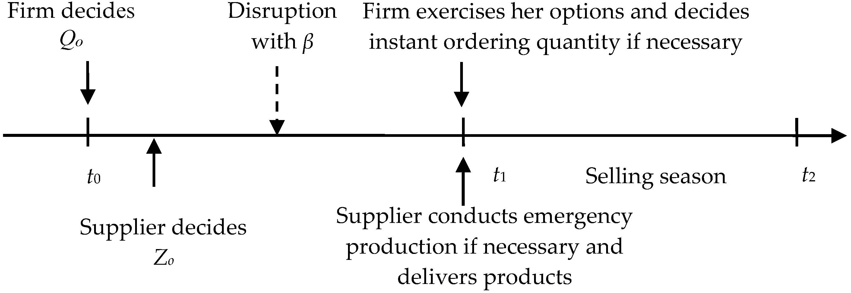
Under the OP strategy (Figure 1), before the selling season, at time t0, the firm decides the option order quantity Qo and the unreliable supplier decides his production quantity Zo afterwards. When the selling season (t1) begins, after the firm observes the realized demand and the emergency procurement price, she exercises the options and decides whether to instant order from the supplier with price p. The option price and exercise price are co and w, respectively. Regarding the unreliable supplier, if he is disrupted or his inventory is not enough, the supplier can carry out emergency production to satisfy the option ordering or emergency ordering. The emergency production here represents the situation where the supplier can work overtime, begin using the backup production line, dig spare capacity, or just use the same or high-end product in inventory for alternative supply [10,30,40]. The supplier’s production cost is c and the emergency production cost is ce (ce > c). All unsold product will be salvaged with price s per unit.
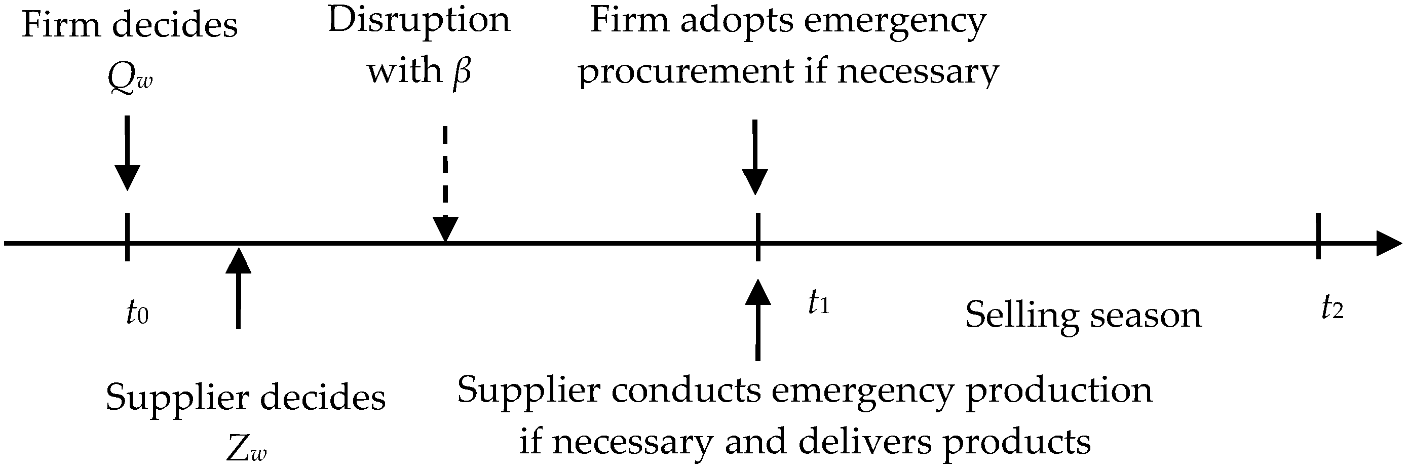
Under the PC strategy (Figure 2), at time t0, the firm first decides the order quantity Qw with wholesale price w. Subsequently, the unreliable supplier decides the production quantity Zw. Once the firm observes the realized demand and emergency procurement price at time t1, she decides whether to instant order from the supplier. When the remnant inventory is enough, her emergency ordering will be satisfied. The authors assume when the instant price is relatively high (p > ce) and the disruption does not happen, the supplier can adopt emergency production to satisfy the firm’s instant ordering.
The authors assume the supplier and firm are both risk-neutral and they have complete information about each other. The relationship between the supplier and the firm is characterized by a Stackelberg game, where the firm acts as the leader and the supplier is the follower. The subscripts “S”, “R”, “o”, and “w” denote the supplier, the firm, the OP strategy, and the PC strategy, respectively. The superscript “*” denotes the optimum.
Throughout this paper, the authors make the following assumptions:
- (1)
- , which ensures the salvage value is lower than the production cost;
- (2)
- and , which ensure the supplier and the firm both have positive profits under the OP strategy;
- (3)
- , which represents the emergency production cost is higher than the normal production cost;
- (4)
- , which ensures the firm can achieve positive profit through instant ordering;
- (5)
- , which denotes the emergency purchase price is higher than the option purchase price;
- (6)
- , which ensures the supplier has a positive profit if he produces.
The authors define: , , , . Then, it is easy to derive the following condition: .
4. Model Analyses
The authors explore the equilibrium production and procurement decisions of the unreliable supplier and the firm under the option purchase (OP) strategy and procurement commitment (PC) strategy, respectively.
4.1. Option Purchase Strategy
4.1.1. Supplier’s Production Decision
Given the firm’s option ordering quantity , let denote the supplier’s profit. When the realized emergency procurement price is lower than the emergency production cost, , then the supplier’s expected profit is:
where the first three terms denote the production cost, the option ordering and final option exercise revenues, respectively; the fourth term is the revenue for satisfying the firm’s emergency procurement; the fifth term represents the salvage value; and the final two terms are the emergency production investments. Due to the low emergency procurement price, the firm’s emergency procurement demand will be met only with leftover inventory. The supplier’s emergency production only is used to satisfy the firm’s possible exercised option ordering.
, then the supplier’s expected profit is:
Due to the high emergency procurement price in this situation, all the firm’s emergency procurement demand will be met by the supplier with normal production and emergency production.
The authors, for convenience, define , , , . Therefore, considering the randomness of the emergency procurement price, the supplier’s expected profit can be given by:
where the first three terms have the same meaning as above; the fourth and fifth terms are the revenues for the possible instant ordering when the emergency procurement price is relatively low and high, respectively; the last four terms are the emergency procurement costs when the disruption occurs and not, and the emergency procurement price is low and high, respectively. The supplier’s expected profit can also be formulated as:
Taken from Equation (4), it can be found that has different forms when or . Exploring the properties of , Lemma 1 can be derived.
Lemma 1.
The supplier’s profit function, is continuous for . Additionally, it is differentiable and concave in for and , respectively.
Let denote the best response function. Based on Lemma 1, by the first order condition, the supplier’s optimal production decision can be derived. Define and satisfying and , respectively.
Theorem 1.
For any option ordering quantity
the supplier’s best response function is
When the option order is moderate (refer to Figure 3), , the supplier’s optimal production quantity is equal to firm’s option ordering quantity. When the option order is relatively big, , the supplier’s optimal production quantity has an upper bound, which is independent of the emergency procurement price. When the option order is relatively small, , the supplier’s optimal production quantity has a lower bound, which is dependent on the emergency procurement price. Furthermore, the upper and lower bounds are decreasing in both disruption risk and production cost, while they are increasing in both emergency production cost and salvage value.
4.1.2. Firm’s Procurement Decision
Let be the firm’s expected profit. is the supplier’s best response when the firm’s option order is . When the realized emergency procurement price is lower than the emergency production cost, , the firm’s expected profit is:
where the first term is the revenue from satisfying the demand with exercised option; the second term is the revenue from emergency procurement; the last two terms are the option exercising and purchasing cost. When the emergency procurement price is relatively low, the firm’s emergency ordering demand can be met only when the disruption does not occur, and the inventory is sufficient.
Similarly, if the realized emergency procurement price is higher than the emergency production cost,
, then the firm’s expected profit is:
where the first two terms are the revenue and last two terms are the costs. Note that, in the condition of , the firm’s emergency procurement will always be satisfied by the supplier’s normal and emergency production. Using Equation (6), it can be seen that the firm’s profit is independent of the supplier’s production quantity and disruption risk.
Considering the randomness of the emergency procurement price and the best response from the supplier, the firm’s expected profit can be expressed by:
where the first two terms are the revenues when and the third term is the revenue when ; the last four terms are the emergency procurement, option exercising, and ordering costs. The firm’s expected profit can also be formulated as:
Taken from Equation (8), has different forms when or . Exploring the properties of , Lemma 2 can be derived as follows.
Lemma 2.
The firm’s profit function, is continuous for . Additionally, it is differentiable and concave in for and , respectively.
As per Lemma 2, through comparing the firm’s optimal profits when and , the optimal decision of the firm can be obtained. To avoid a trivial case, the authors assume . Defining and satisfying and , the optimal decisions of the supplier and the firm can be derived as follows.
Theorem 2.
Under the OP strategy, the firm’s optimal option procurement quantityand the supplier’s optimal production quantitysatisfy the following conditions:
- (i)
- when , then , ;
- (ii)
- when , , ;
where , satisfies , satisfies , and can be formulated as:
Corollary 1.
,,,;,,;,,;,,,.
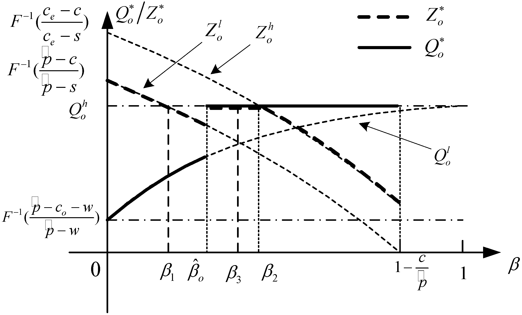
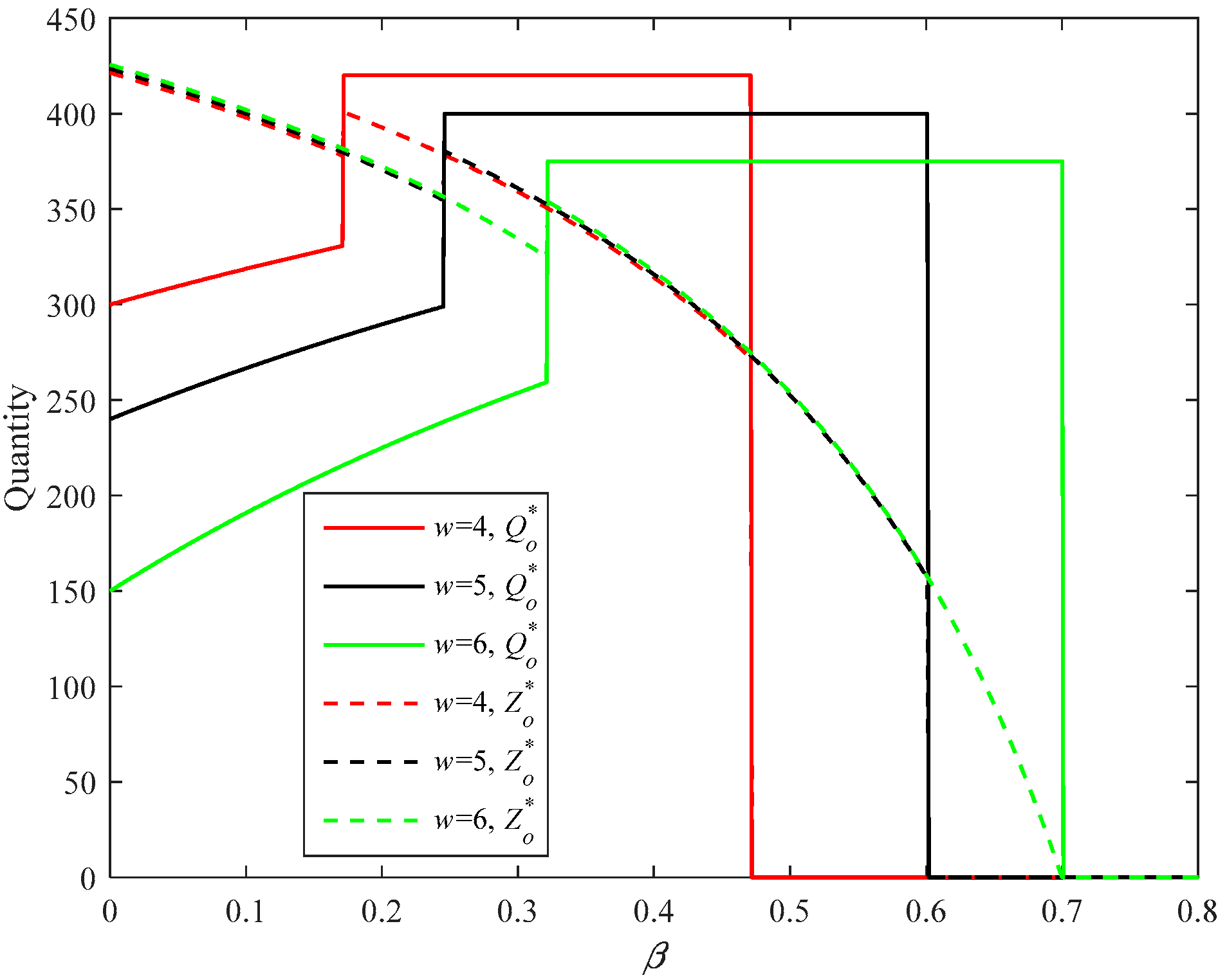
Figure 4 gives a graphic description of Theorem 2. Found in Figure 4, and are the critical points when and , respectively. Note that whether is bigger than or not is uncertain. Figure 4 describes the cases of . Looking at Theorem 2 and Figure 4, there also exist upper and lower bounds for . When , and take their lower bounds and , respectively. Accompanying the increase of the disruption risk, increases, whereas decreases (refer to Corollary 1). When , takes its upper bound , and takes its upper bound or is equal to . Occurring in this situation (refer to Corollary 1), is a constant and is independent of disruption risk. However, is non-increasing in the disruption risk.
The following managerial insights can be derived. Using the OP strategy, the firm’s optimal procurement quantity can be represented by two newsvendor solutions ( and can be considered as the retail prices). The firm’s procurement follows a “threshold” principle. When the disruption risk is less than the threshold, the firm’s optimal procurement quantity takes the lower newsvendor solution (or lower bound); otherwise, it takes the higher newsvendor solution (or upper bound). Similarly, for the unreliable supplier, his optimal normal production quantity takes the production lower bound when the disruption risk is lower than the threshold; it is equal to the firm’s option ordering quantity or takes the production upper boundary otherwise. Moreover, the firm’s optimal procurement quantity is non-decreasing, whereas the supplier’s optimal production quantity is non-increasing in the disruption risk when the disruption risk is lower and higher than the threshold, respectively.
4.2. Procurement Commitment Strategy
4.2.1. Supplier’s Production Decision
Given the firm’s order quantity , let denote the supplier’s expected profit. When the realized emergency procurement price is lower than the emergency production cost, , then the supplier’s expected profit is:
where the first term is the production cost; the second and third terms are the revenues from normal ordering and emergency ordering when disruption does not occur; and the last term is the salvage value. Due to low emergency procurement price, the supplier only will use its leftover inventory to satisfy the firm’s instant ordering. It is easy to know that the supplier will pick () to maximize the following profit:
Similarly, if the realized emergency procurement price is no lower than the emergency production cost, , the supplier will satisfy all the firm’s instant ordering when he is not disrupted, then the supplier’s expected profit is:
Due to the high emergency procurement price, the supplier will fully satisfy the firm’s instant ordering if he is not disrupted. Concerning the supplier, he will always choose , then the supplier’s expected profit can be formulated as:
Considering the randomness of the emergency procurement price, the supplier’s expected profit can be given by:
Equation (13) can also be expressed by:
Let denote the supplier’s best response function. It is easy to verify that is concave in . Define satisfying . Using the first order condition, the supplier’s optimal production decision can be derived.
Theorem 3.
For any firm’s order quantity Qw, the supplier’s best response function is:
Corollary 2.
Regarding the supplier, his optimal production quantity has a lower bound, which is equal to his optimal production lower bound under the OP strategy. Similarly, the lower bound is decreasing in disruption risk. When the firm’s ordering is less than the lower bound, the supplier’s optimal production quantity takes the lower bound, otherwise, it is equal to the firm’s ordering quantity.
4.2.2. Firm’s Procurement Decision
Let be the firm’s expected profit. When the realized emergency procurement price is lower than the emergency production cost, , then the firm’s expected profit is:
Here, the first term is the normal ordering cost. The second term is the revenue for satisfying the market demand. The third term is the expense for emergency procurement. The last term is the salvage value. Note that the firm’s emergency ordering is only satisfied with the leftover inventory of the supplier.
Similarly, if the realized emergency procurement price is no lower than the emergency production cost, , then the firm’s expected profit is:
The difference between Equations (15) and (16) is, due to the high emergency procurement price, all the firm’s emergency procurement demand always will be satisfied by the supplier if he is not disrupted.
Considering the randomness of the emergency procurement price, the firm’s expected profit can be formulated as:
where the term is the normal purchase expense; the second and third terms are the revenue when the emergency procurement price is lower and higher than the emergency production cost, respectively; the fourth and fifth terms are the emergency procurement costs when the emergency procurement price is relatively lower and higher, respectively; and the last term is the salvage value. The firm’s expected profit can also be expressed by:
Define and satisfying and , respectively. The optimal decisions of the supplier and the firm under the PC strategy can be derived as follows.
Theorem 4.
Under the PC strategy, the firm’s optimal procurement quantityand the supplier’s optimal production quantity satisfy the following conditions:
- (i)
- if, then, ;
- (ii)
- if, then, wheresatisfies,satisfiesandcan be formulated as:
Corollary 3.
.
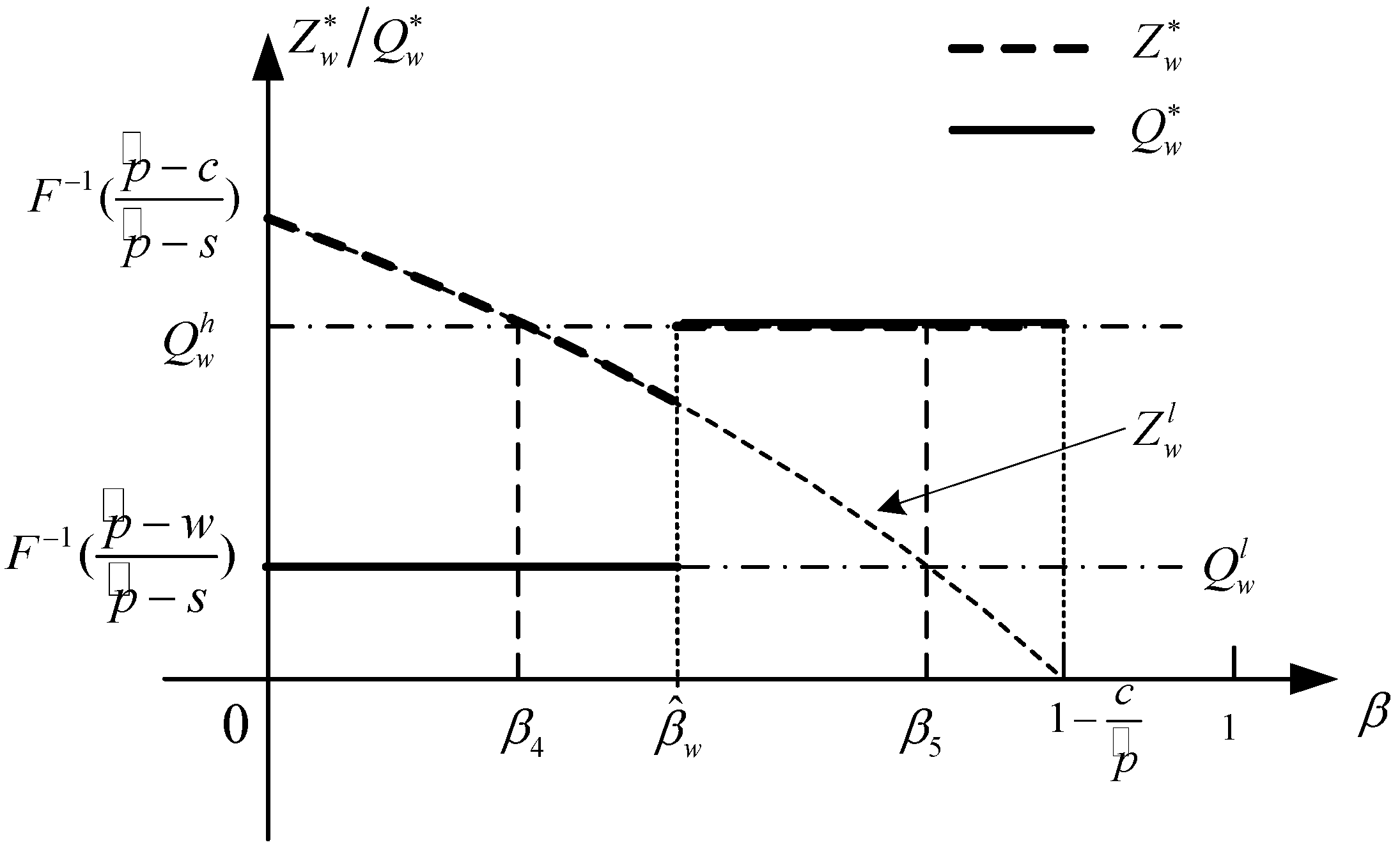
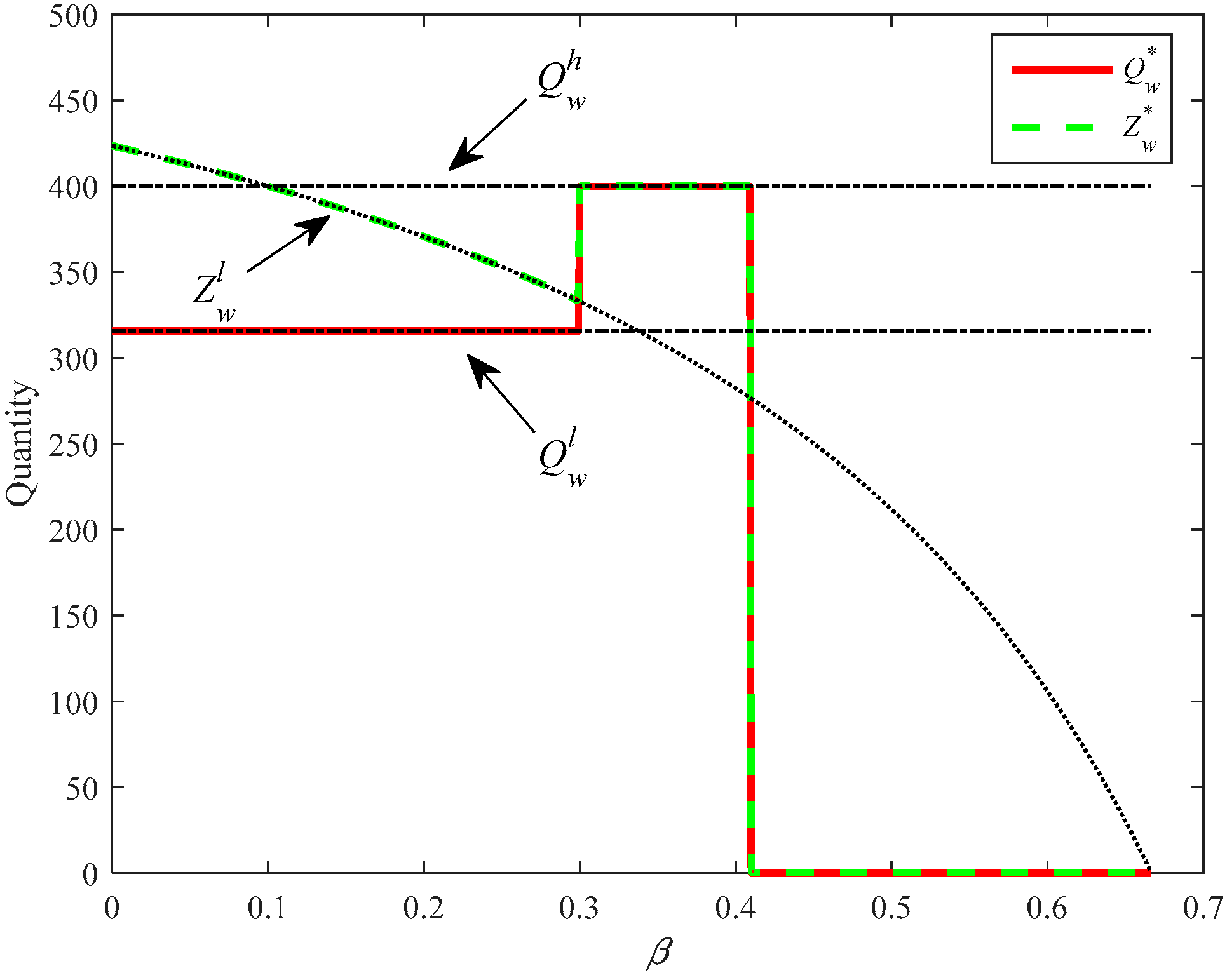
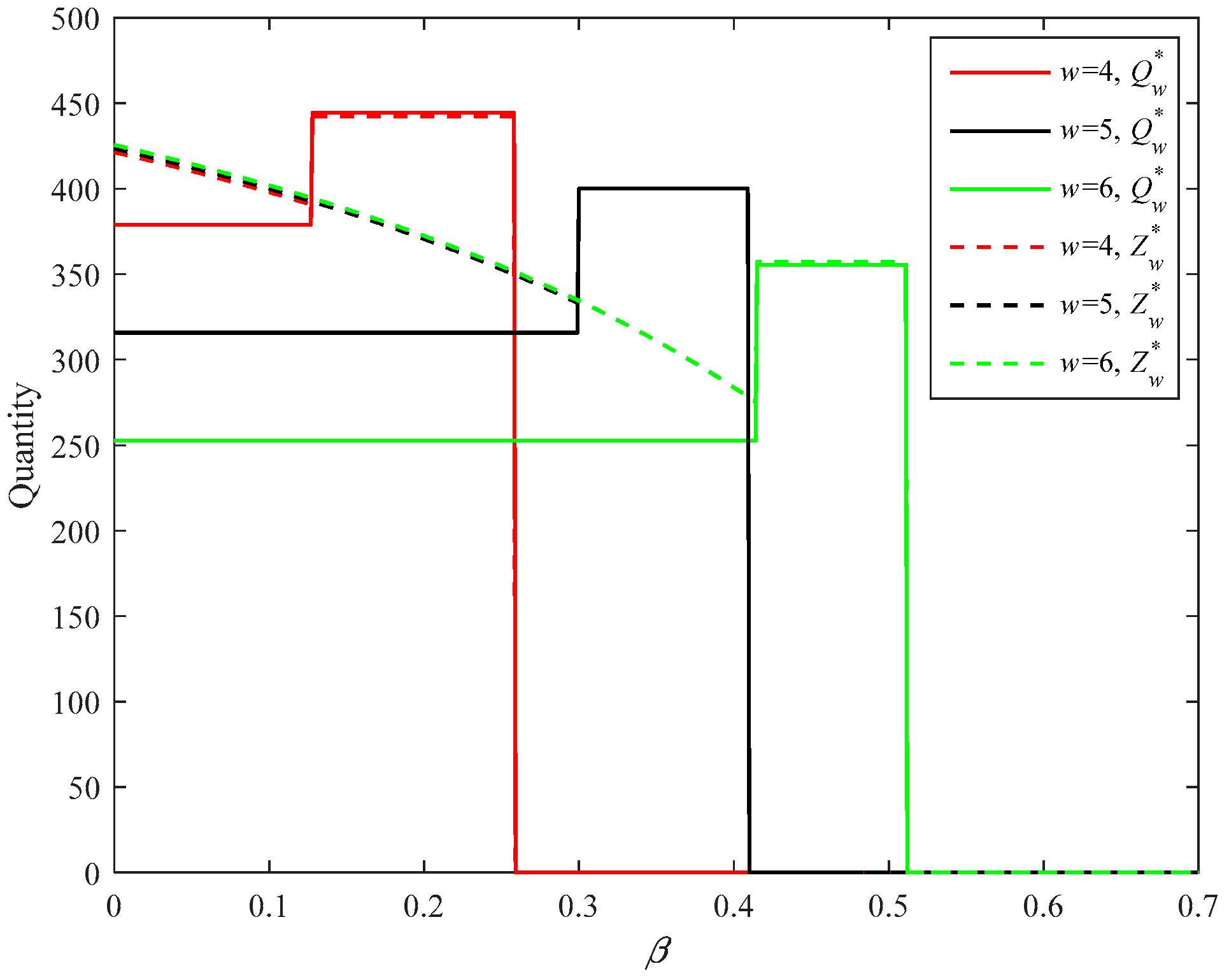
Figure 5 gives a graphic description of Theorem 4. and are the critical points when and , respectively. Looking at Theorem 4 and Figure 5, there also exist upper and lower bounds for . The two bounds are the newsvendor solutions ( and can be considered as the retail prices) and they are independent of the disruption risk. When , and take their lower bounds, and , respectively. When the disruption risk increases, decreases (refer to Corollary 3). When , takes its upper bound , and is equal to . Considering this situation (refer to Corollary 3), and are both constants and are independent of disruption risk.
Using the PC strategy, the firm’s procurement also follows a “threshold” principle. When the disruption risk is less than the threshold, the firm’s optimal procurement quantity takes the lower newsvendor solution (or lower bound); otherwise, it takes the higher newsvendor solution (or upper bound). Similarly, for the unreliable supplier, his optimal normal production quantity takes the production lower bound when the disruption risk is lower than the threshold; and it is equal to the firm’s normal ordering quantity otherwise.
5. Comparisons
The authors compare the supplier’s and the firm’s optimal decisions and profits under option purchase (OP) strategy and procurement (PC) strategy, respectively and also explore the impacts of some important model parameters. Furthermore, the firm’s optimal strategy selection decision is given.
Due to the complexity of the optimal decisions (refer to Theorems 2 and 4), it is hard to analyze the optimal profits and explore the impacts of model parameters under the two types of strategies, in theory. To achieve more managerial insights, the authors conduct numerical simulation to compare the two types of strategies. The numerical examples are based on the following combination of parameters: s = 0.5, c = 3, co = 3, w = 5, A = 6, B = 14, ce = 10, r = 16, P∼U (6, 14), and demand ζ∼U (0, 600). The values of these parameters are set based on assumptions (1)–(6) presented in Section 3 and previous literature in the area (refer to [33,34,35]). The authors also conduct numerical experiments with other combinations of parameters, the results of which show that the main conclusions and analytical results in this study are robust.
5.1. Optimal Decisions and Profits of the Supplier and Firm under the Two Types of Strategies
5.1.1. Impact of β
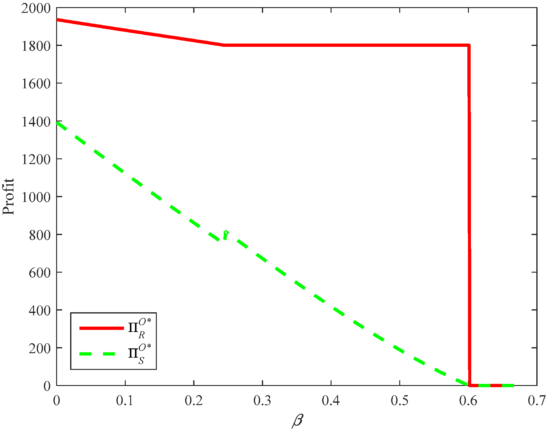
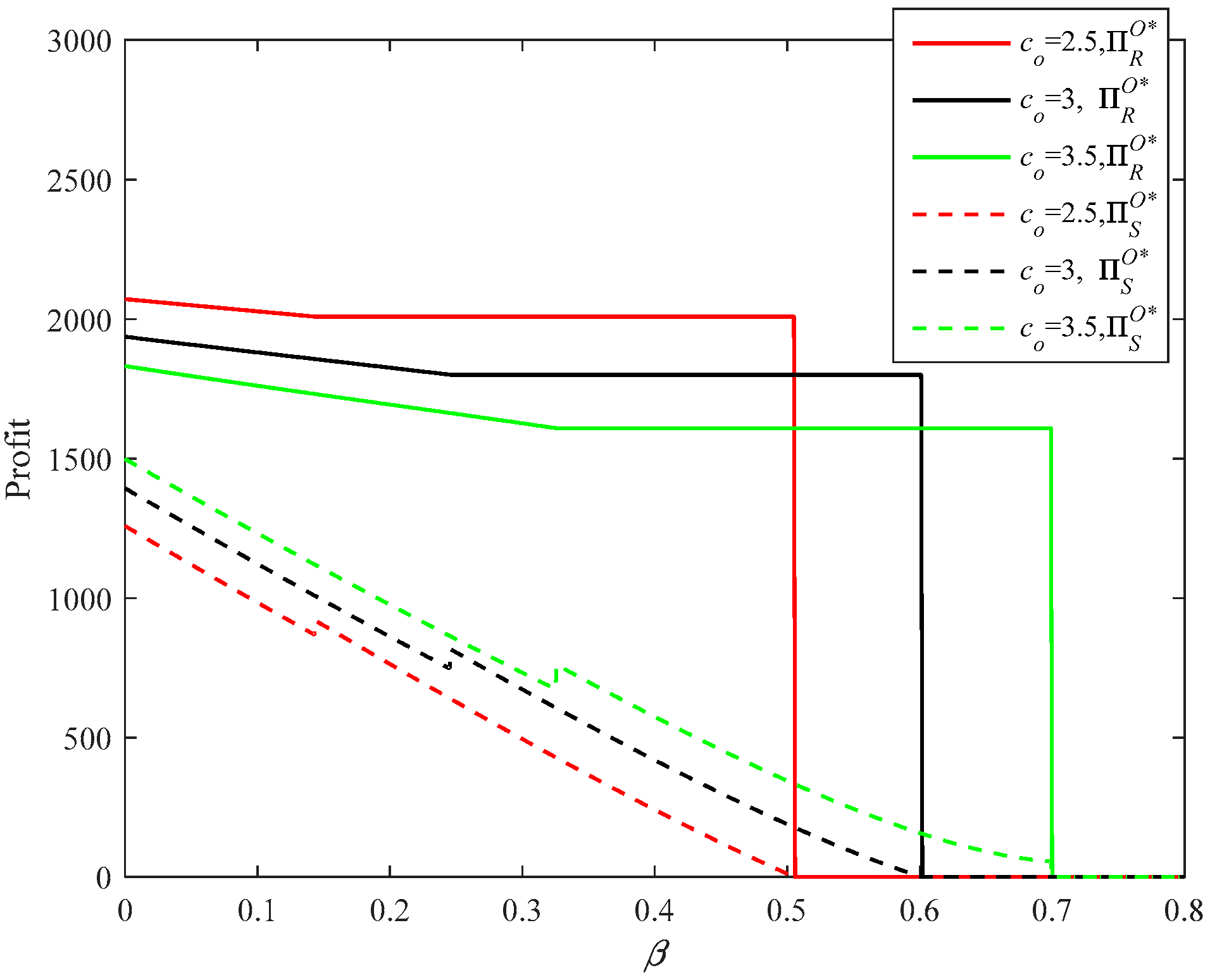
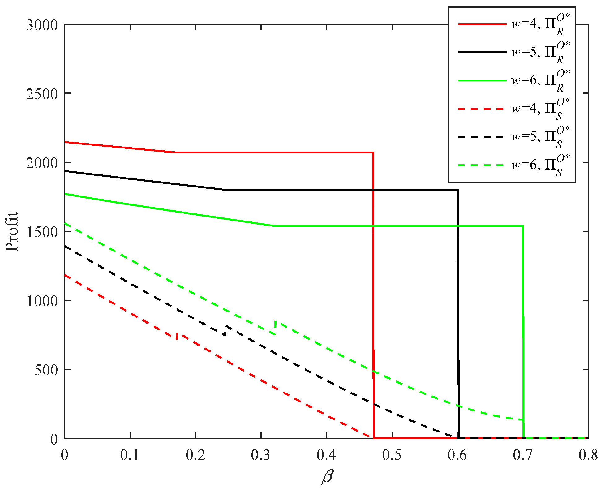
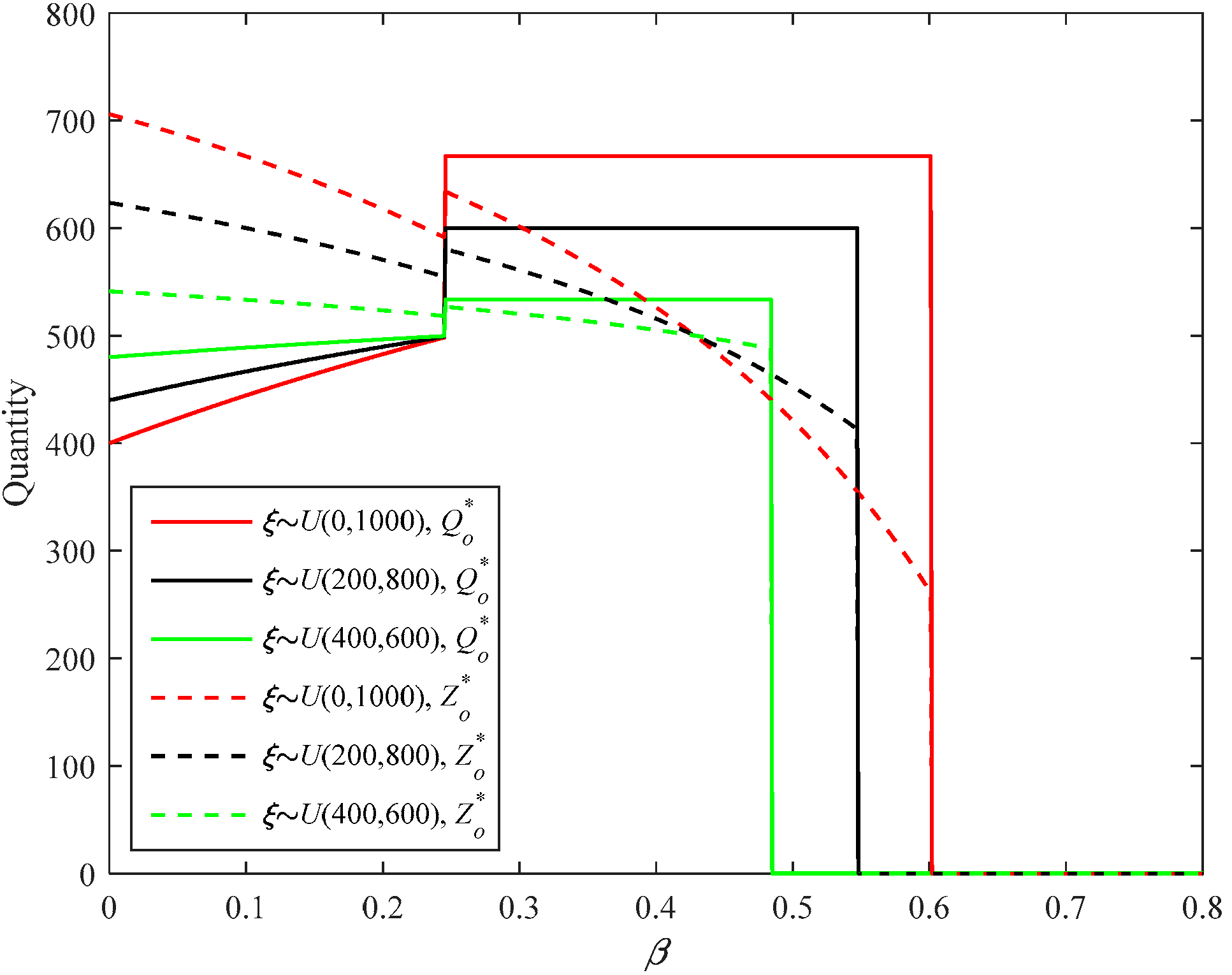
Using the OP strategy (Figure 6 and Figure 7), the firm’s option ordering quantity is non-decreasing, while her profit is non-increasing in disruption risk. This shows that, with the increase of the disruption risk, the benefit of the emergency procurement decreases, and the firm tends to reserve more options to deal with the increasing disruption risk. When the disruption risk is above a threshold, the firm’s option ordering and profit become a constant. When in this situation, the OP strategy can protect the firm from any disruption risk. For the supplier, his production quantity and profit both decrease with the disruption risk, either when the disruption risk is lower or higher than a threshold. This implies that the supplier tends to produce less to mitigate the increasing supply disruption risk. Counterintuitively, the supplier’s production quantity and profit might rise when the disruption risk exceeds a threshold. This is mainly because the supplier needs a rise in production to deal with the firm’s changes in option ordering when the disruption risk exceeds a threshold. The supplier will benefit from this increase in production, thus his profit will rise too.
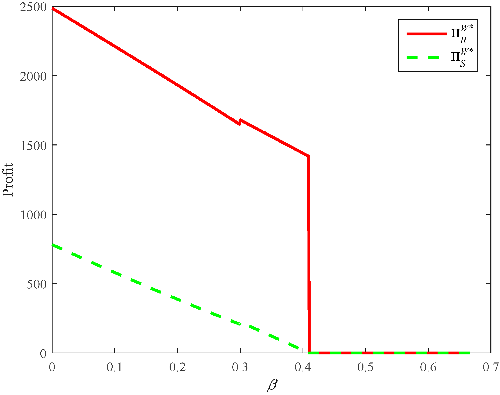
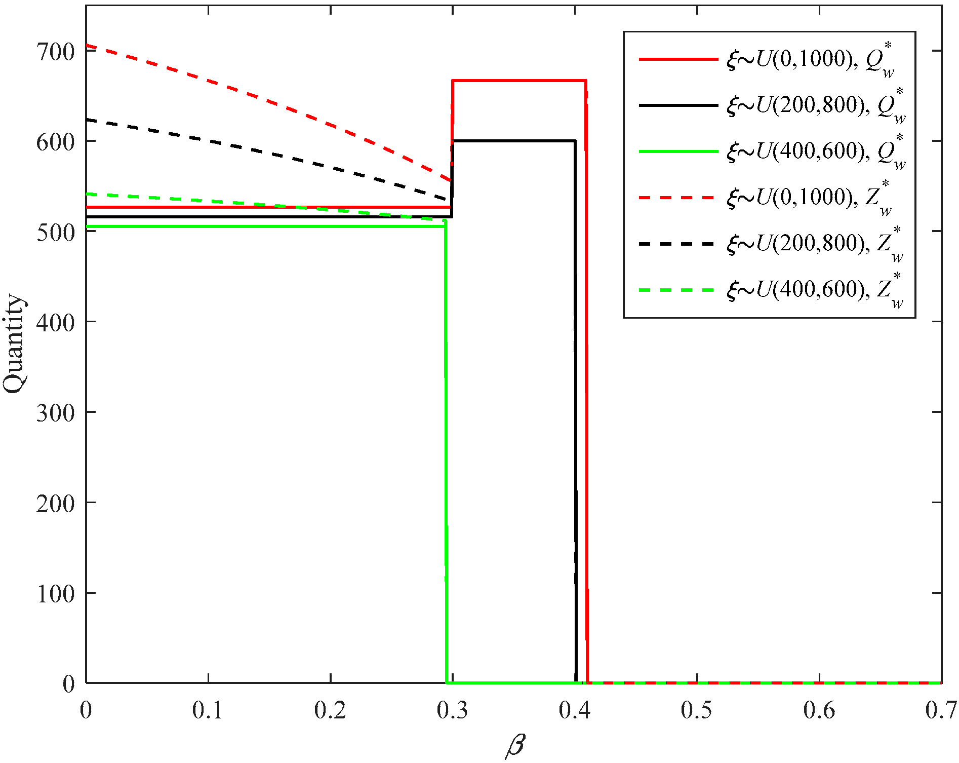
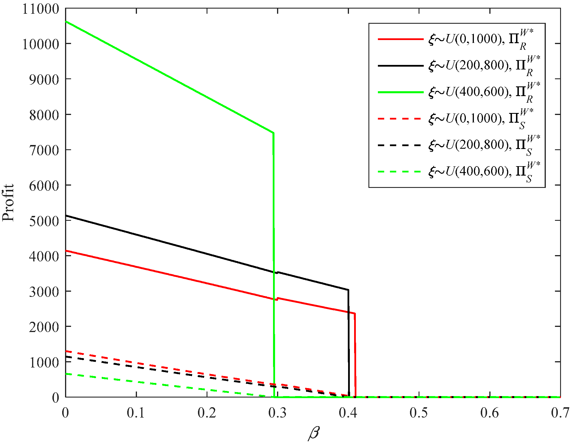
Using the PC strategy (Figure 8 and Figure 9), when the disruption risk is relatively low, the supplier has an incentive to produce more products to satisfy the firm’s possible instant ordering, but the motivation becomes lower with the increase of disruption risk. Regarding the firm, her normal ordering is relatively low, and she can rely more on the emergency procurement to satisfy market demand. When the disruption risk exceeds a threshold, the firm’s order quantity changes from a low newsvendor quantity to a high newsvendor quantity. When in this situation, the supplier has no incentive to produce more products than that ordered. Concerning the firm, she raises her normal ordering to satisfy the demand. Generally, the disruption risk has a negative influence on the supplier’s and firm’s profits. However, the firm’s profit might rise when the disruption risk exceeds a threshold. This implies that the firm will benefit from the rise of her ordering quantity.
5.1.2. Impacts of co, w, and ce
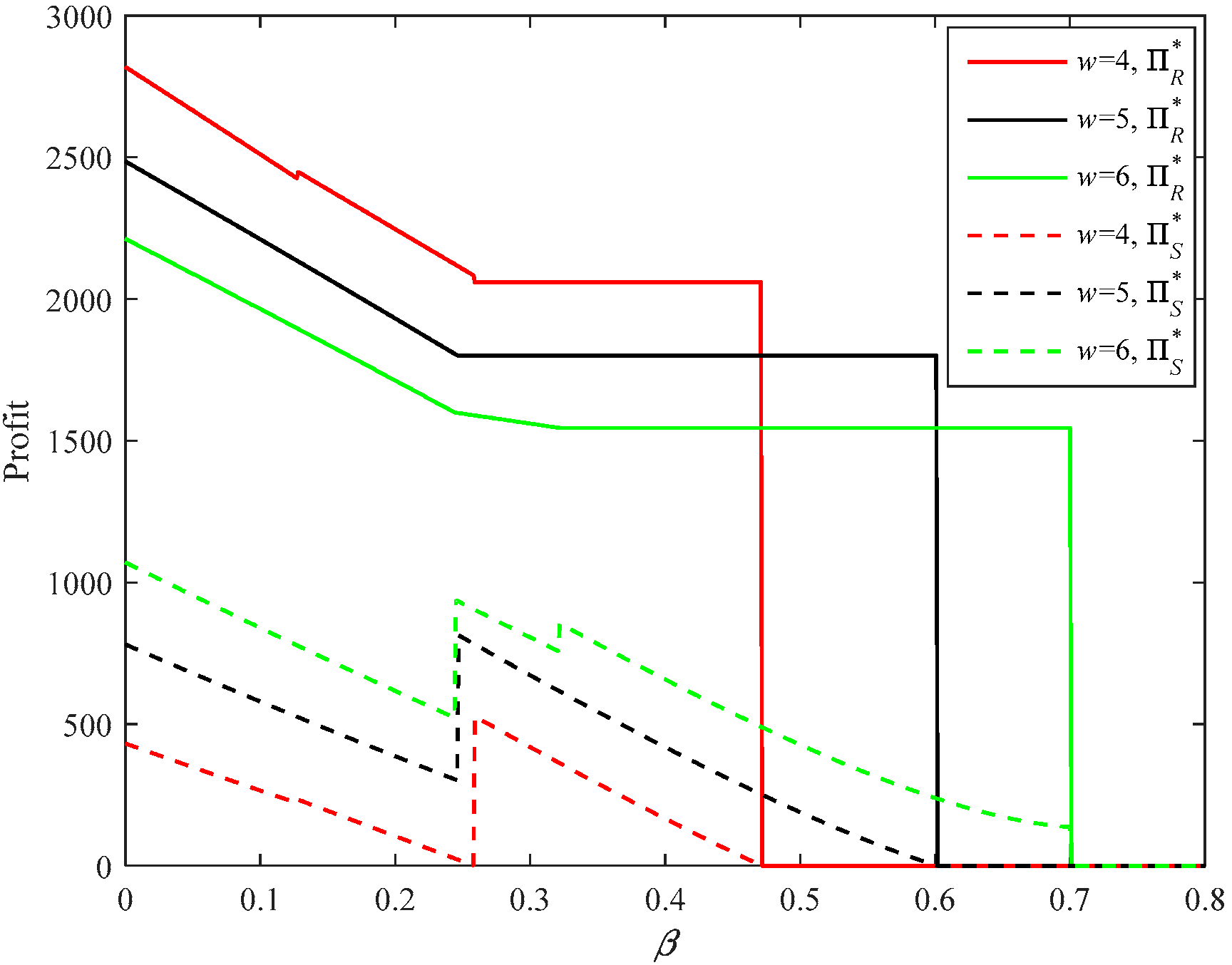
Figure 10, Figure 11, Figure 12, Figure 13, Figure 14 and Figure 15 describe the impacts of option price, co, and exercise price, w, on the supplier’s and firm’s optimal decisions, and the profits under the two types of strategies. Under the OP strategy, the option price and exercise price have a similar influence on the optimal decisions and profits of the supplier and firm. The option price and exercise price have no influence on the supplier’s production upper bound and lower bound, but a lower option price or option exercise price can raise the upper and lower bounds of the firm’s option ordering. Moreover, a lower option price or exercise price benefits the firm, while it damages the supplier. Accompanying the increase of the option price or exercise price, the supplier has an incentive to cooperate with the firm in a riskier operational environment.
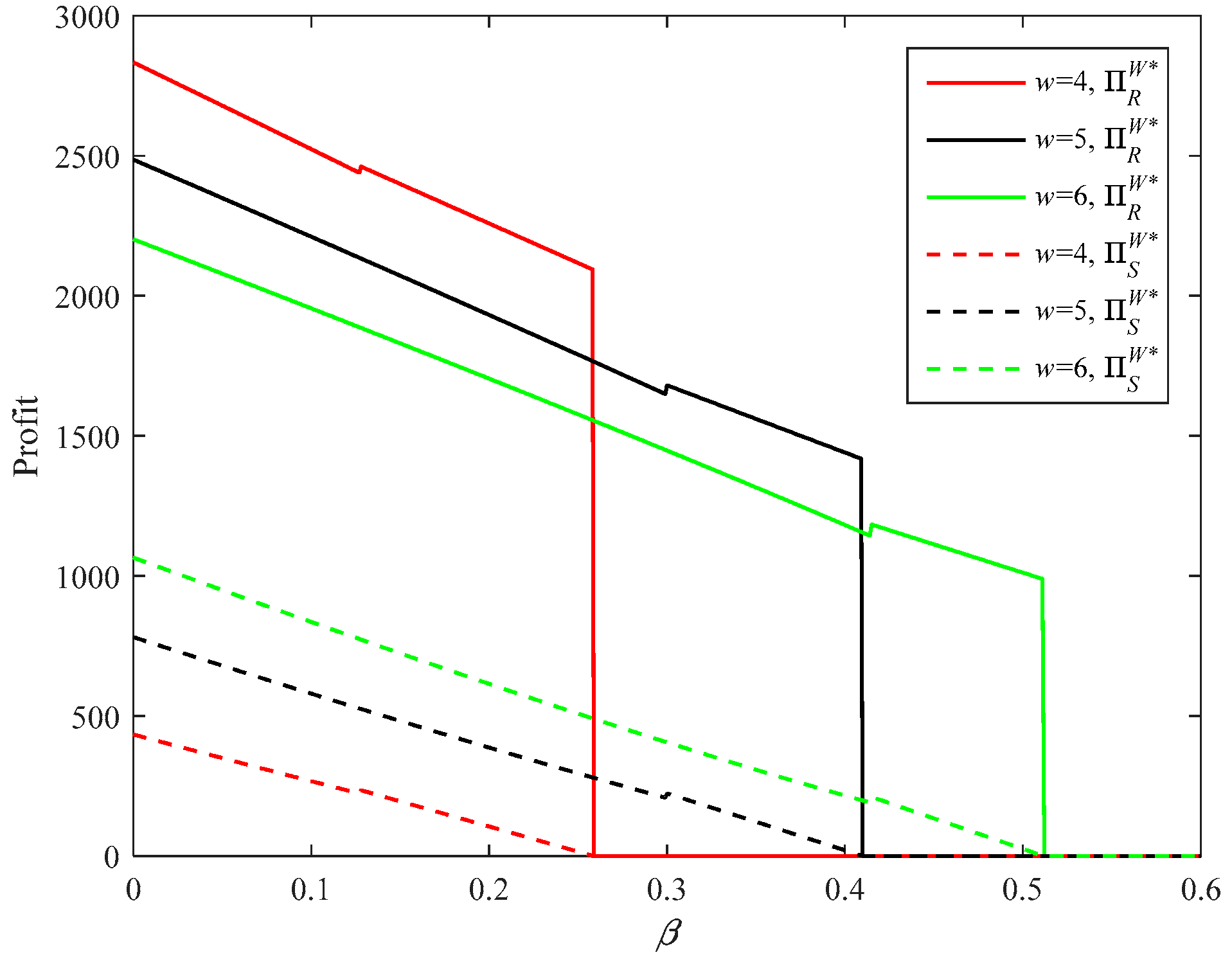
Similarly, under the PC strategy, the wholesale price has no impact on the production lower bound of the supplier, but a lower wholesale price will raise the upper and lower bounds of the firm’s normal ordering. Alongside the increase of the wholesale price, the supplier also has incentive to cooperate with the firm in a riskier operational environment.
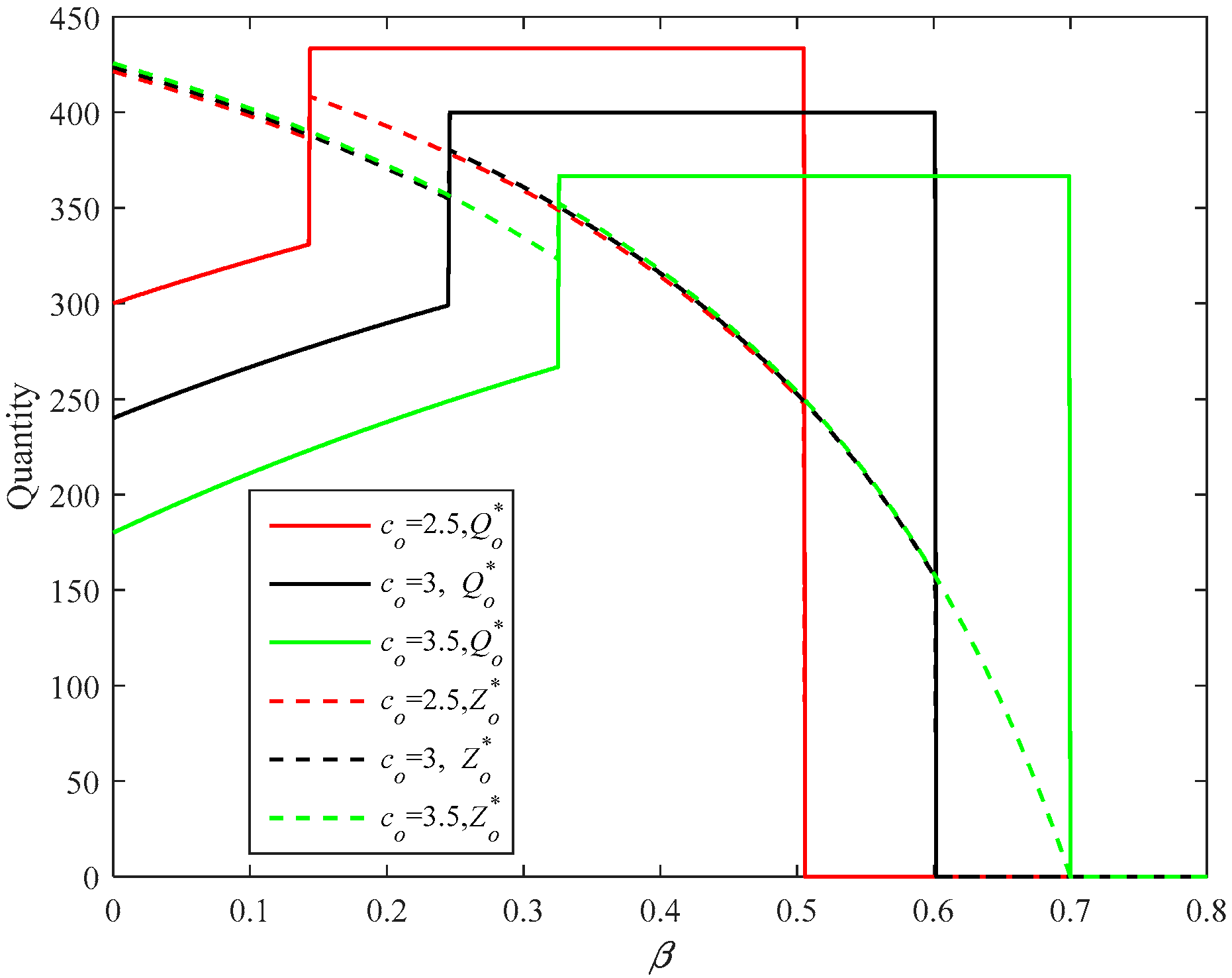
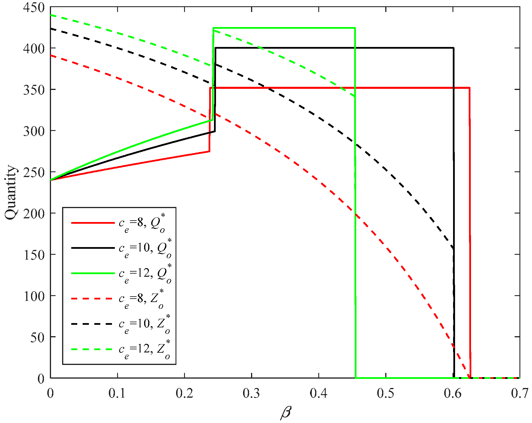
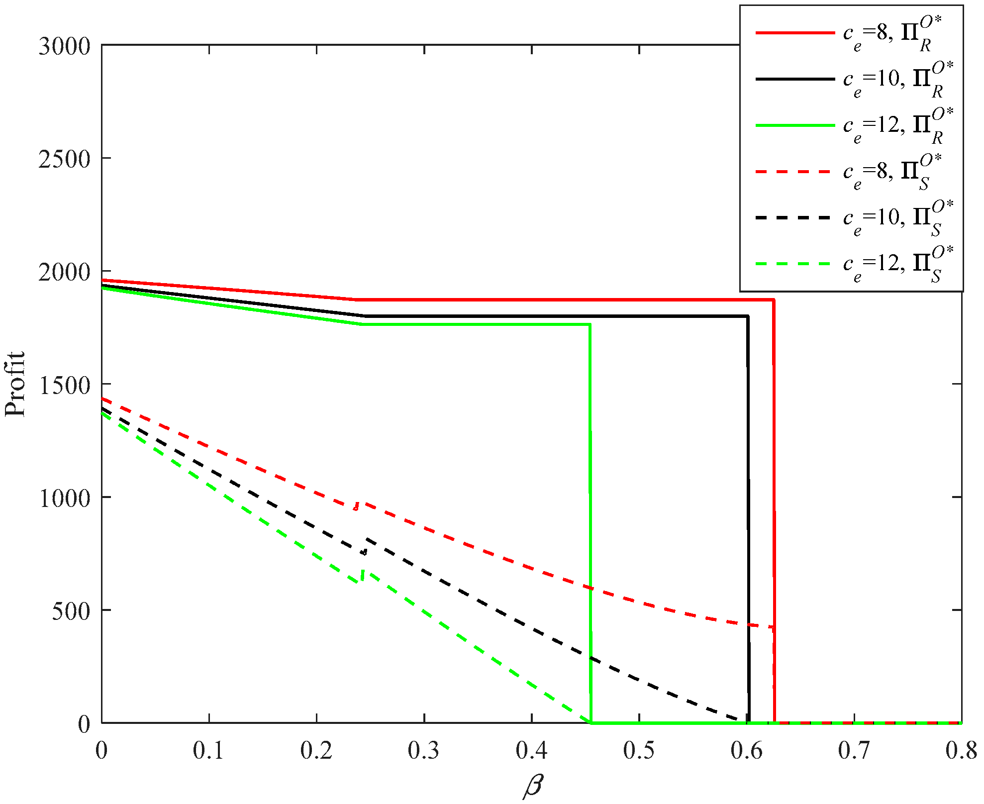
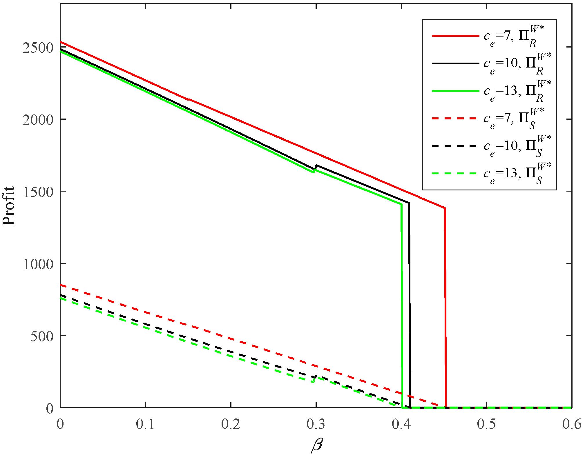
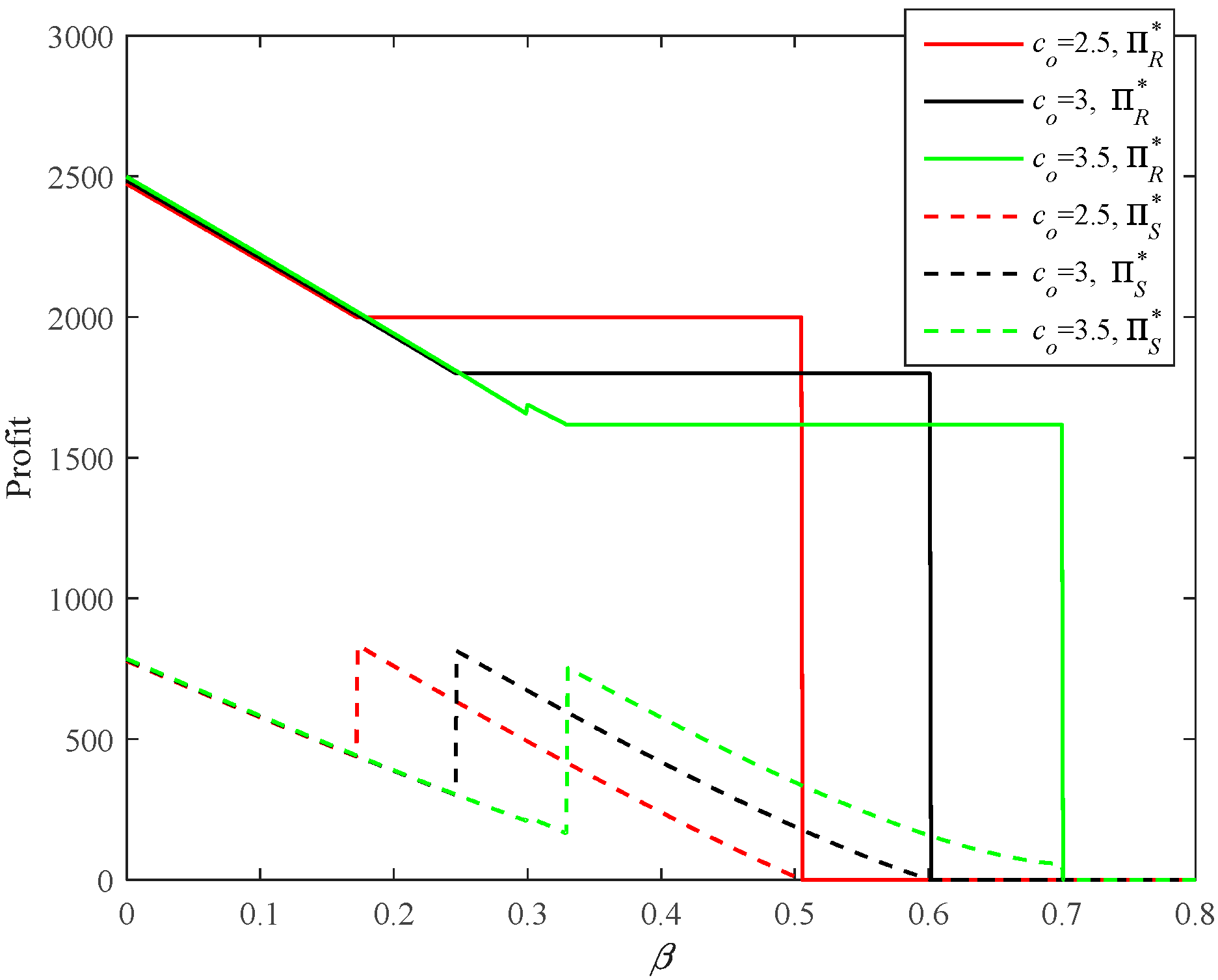
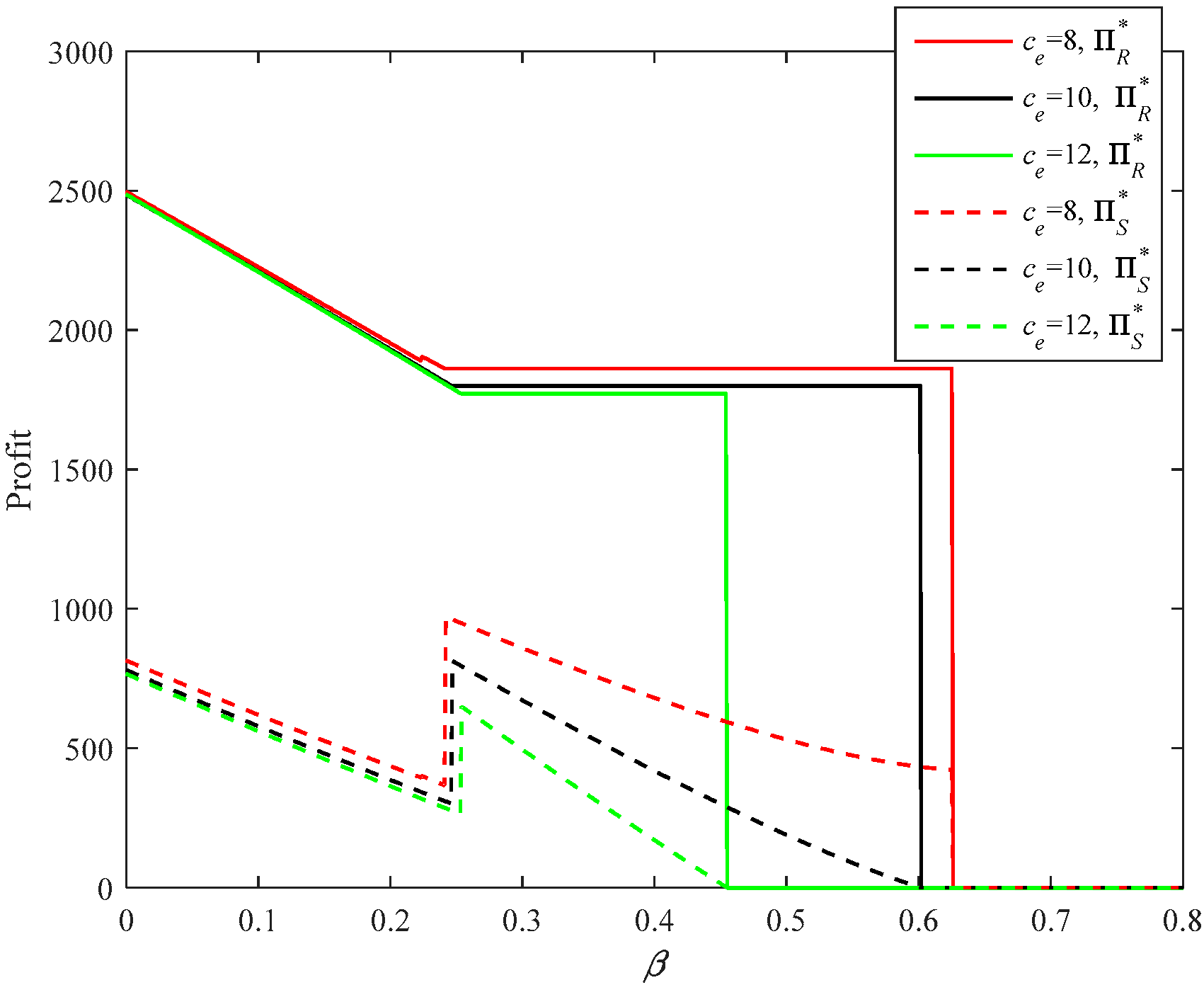
Figure 16, Figure 17, Figure 18 and Figure 19 describe the impacts of emergency production cost, ce, on the optimal decisions and profits under different strategies. Under the OP strategy, a higher emergency production cost will raise the upper and lower bounds of the firm’s option ordering and the supplier’s production. Both the supplier’s and the firm’s profits are decreasing in the emergency production cost. This implies that a higher emergency production cost will impel the supplier and firm to rely more on normal production and normal option ordering, respectively. A higher emergency production cost always has a negative impact on the unreliable supplier and firm.
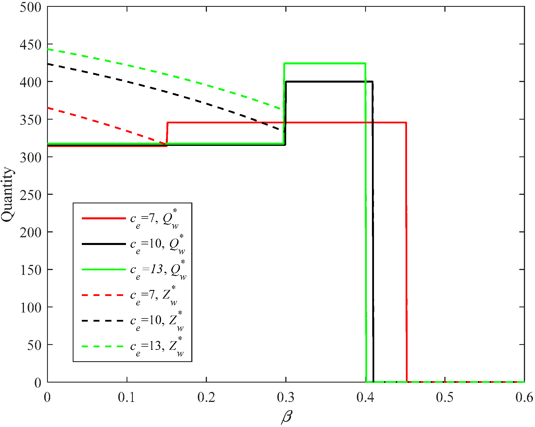
Under the PC strategy, a higher emergency production cost will raise the lower bounds of the supplier’s production and the upper bound of the firm’s normal ordering. It has no impact on the lower bound of the firm’s normal ordering. That is to say, with the increase of the emergency production cost, the supplier relies more on the normal production. Regarding the firm, only when the disruption risk is relatively high does she rely more on the first ordering opportunity. Similarly, a higher emergency production cost will damage both the supplier’s and the firm’s profits. Therefore, reducing the emergency production cost can improve the supply chain member’s profit.
5.1.3. Impacts of P and ζ
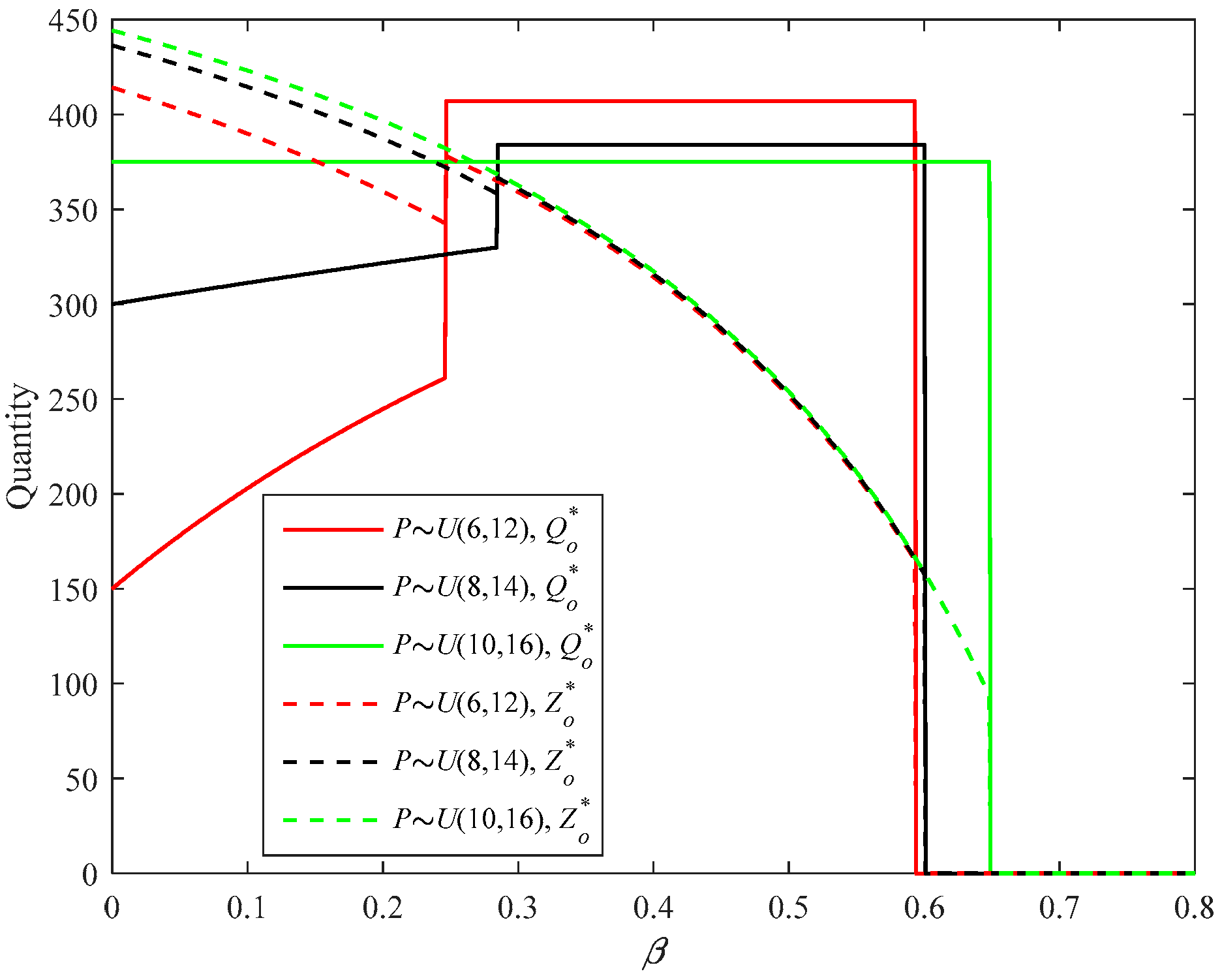
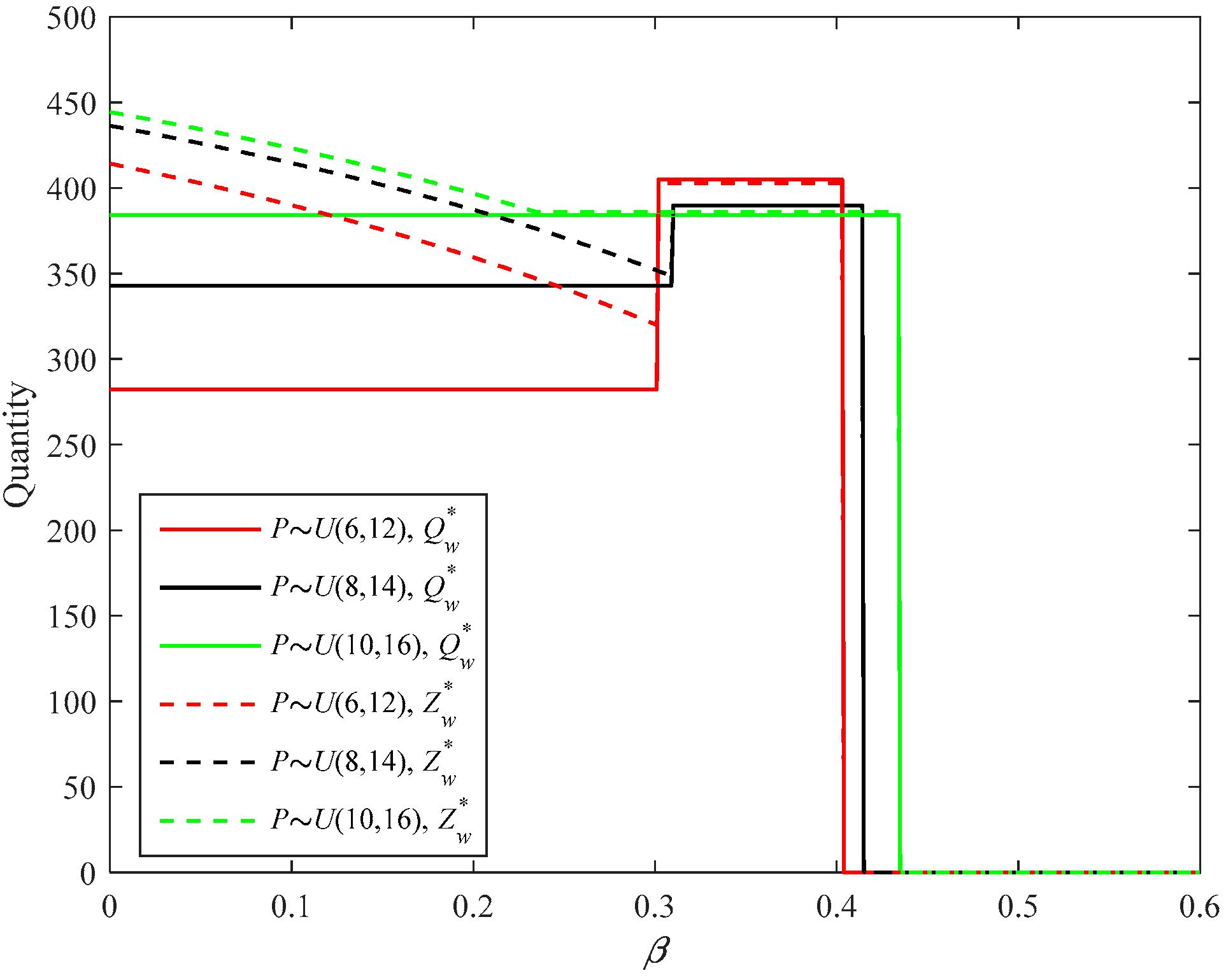
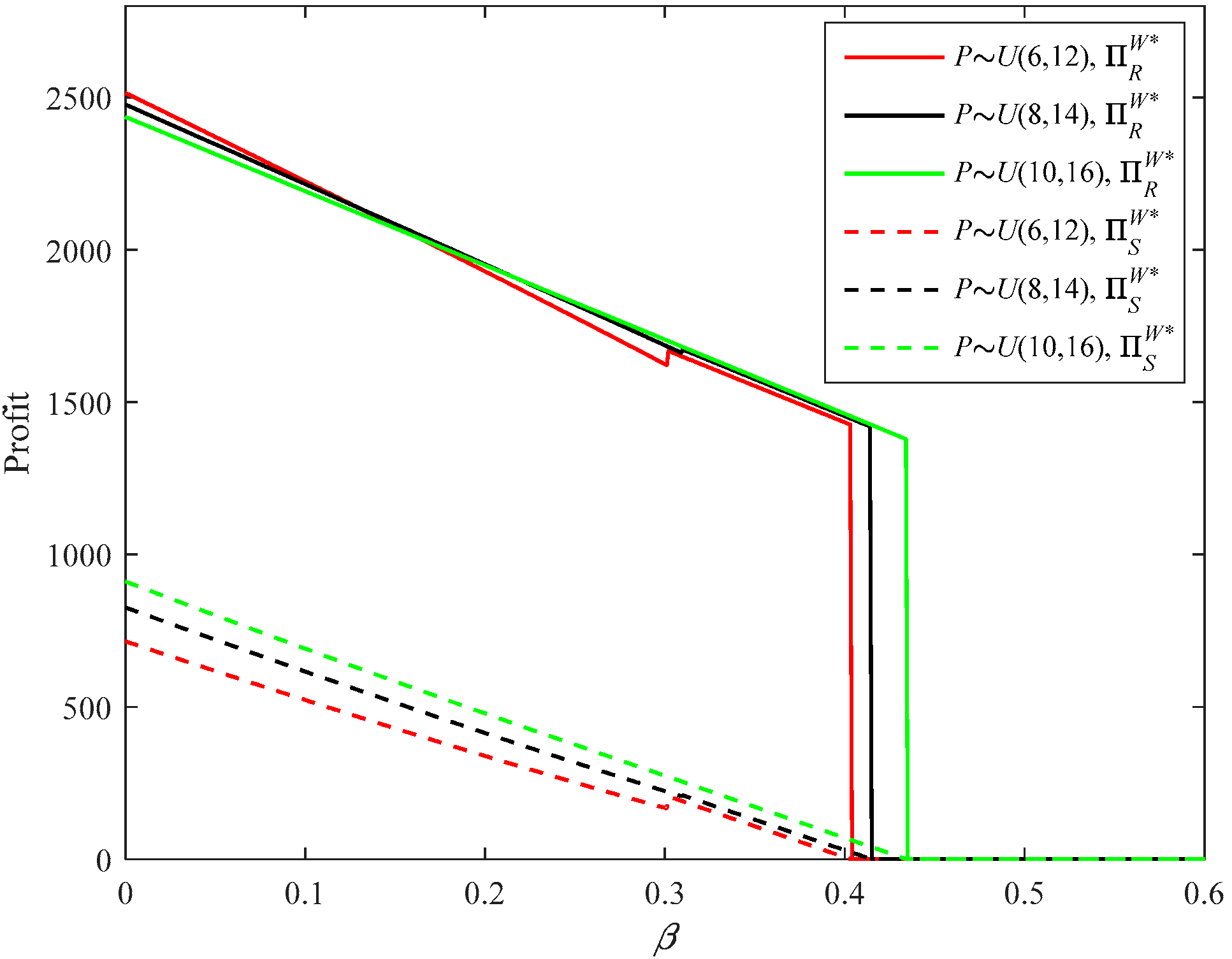
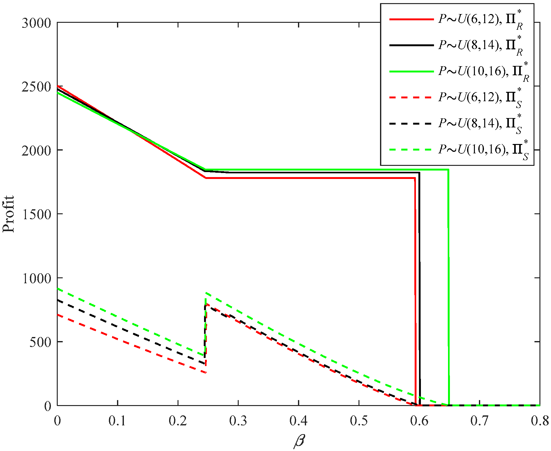
Figure 20, Figure 21, Figure 22 and Figure 23 describe the impacts of the mean value (MV) of emergency procurement price on the optimal decisions and profits under two types of strategies. Under the OP strategy, with the increase of the MV of emergency procurement price, the lower bounds of the supplier’s production and the firm’s option ordering increase; the upper bound of the supplier’s production remains unchanged; whereas the upper bound of the firm’s option ordering decreases. Similarly, under the PC strategy, with the increase of the MV of emergency procurement price, the lower bounds of the supplier’s production and the firm’s normal ordering increase, while the upper bounds of the supplier’s production and the firm’s normal ordering decrease.
Under both strategies, it is natural to find that a higher MV of emergency procurement price is beneficial to the supplier. This is mainly because a higher MV of emergency procurement price often means the firm must pay more to the supplier. However, a lower MV of emergency procurement price is not always beneficial to the firm. When disruption risk is relatively low, the firm benefits from a lower MV of emergency procurement price; otherwise, a higher MV of emergency procurement price is better for the firm. This is counterintuitive and the authors provide an explanation as follows. When the disruption risk is relatively high, the supplier’s optimal production quantity is no more than the firm’s optimal option or normal ordering quantity. The firm has no possibility to adopt emergency procurement due to no leftover inventory. Then the firm pays nothing for the emergency procurement. Moreover, a higher MV of emergency procurement price will impel the firm to reduce her option or normal ordering quantity. The firm will benefit from dealing with demand risk efficiently. Therefore, when disruption risk is relatively high, the firm can benefit from a higher MV of emergency procurement price.
Figure 24, Figure 25, Figure 26 and Figure 27 describe the impacts of market demand variability (VAR) on the optimal decisions and profits under two types of strategies. Using the OP strategy, with the increase in the market demand variability, the lower boundary of the firm’s option ordering decreases, whereas her upper bound increases; the lower and upper bounds of the supplier’s production both increase. Generally, a higher market demand variability is harmful to both the supplier and firm.
Using the PC strategy, with the increase in the market demand variability, the lower bound of the supplier’s production and the lower and upper bounds of the firm normal ordering all increase. A higher market demand variability is harmful to the firm. However, it is interesting to find that the supplier could benefit from a higher market demand variability. This implies that the supplier benefits more from over-production than the damages from the increase in the market demand variability.
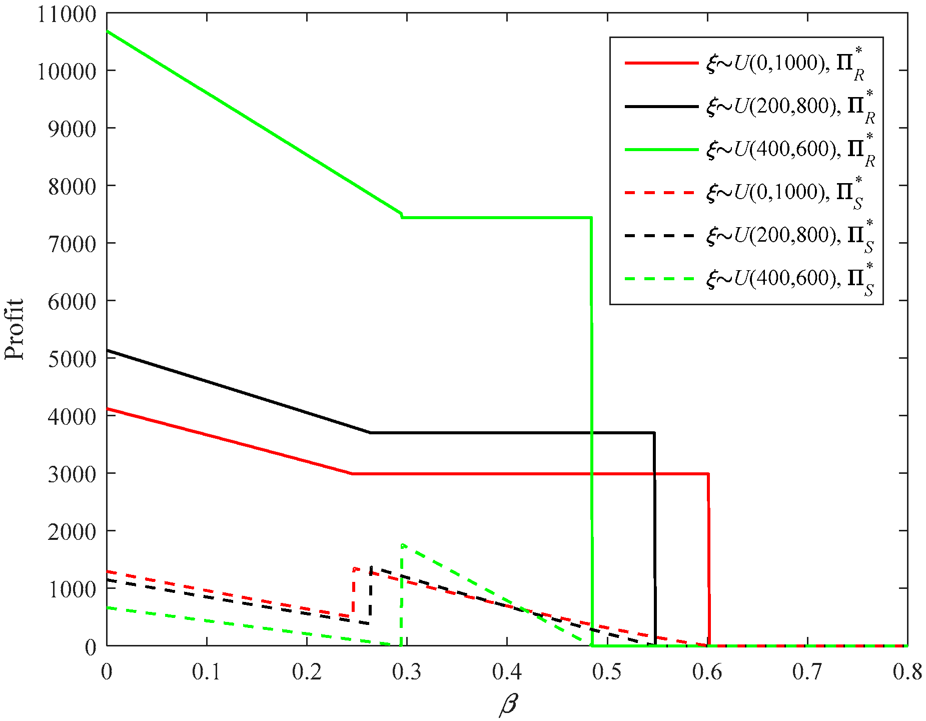
5.2. Firm’s Strategy Selection Decision
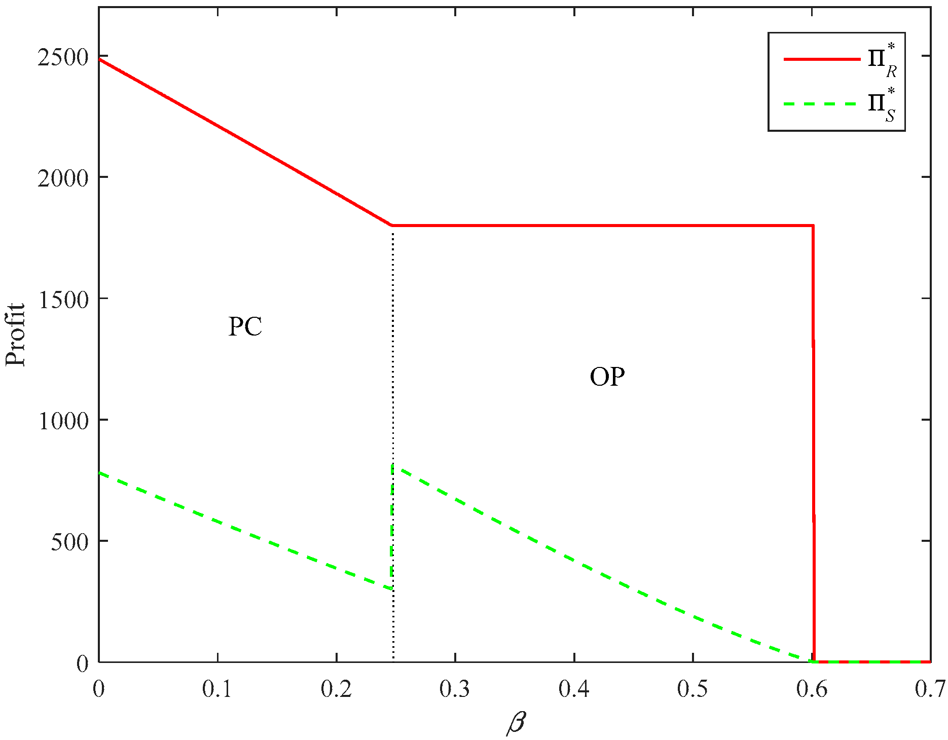
Figure 28 gives the firm’s optimal strategy selection with different disruption risks. When the disruption risk is relatively low, the firm would like to choose the PC strategy. When the disruption risk increases, the firm switches to choose the OP strategy. Moreover, the firm’s profit is non-increasing in disruption risk. Regarding the supplier, his profit decreases with the increase of the disruption risk, in general. However, when the firm switches from the PC strategy to the OP strategy, the supplier’s profit has an increase.
Figure 29, Figure 30 and Figure 31 describe the impacts of the option price and exercise price, as well as the emergency production cost on the firm’s strategy selection. Alongside the increase of the option price, the firm is more likely to choose the PC strategy when the disruption risk is relatively low. A higher option price can assure the supplier to cooperate with the firm under the OP strategy, even if the disruption risk is relatively high. The varying of option exercise price and emergency production cost influences the supplier’s and firm’s profits, whereas it has no influence on the firm’s strategy selection from the risk perspective.
Figure 32 and Figure 33 describe the impacts of the uncertainty of the emergency procurement price and the market demand variability on the firm’s strategy selection. Viewing Figure 32, the varying of MV of the emergency procurement price also does not influence the firm’s strategy selection. Looking at Figure 33, with the increase in the market demand variability, the firm is more likely to choose the OP strategy with the increase of the disruption risk. This is mainly because the OP strategy can help to mitigate both the supply risk and demand risk [34]. Moreover, a higher market demand variability can impel the supplier to cooperate with the firm, even if the disruption risk is relatively high.
6. Conclusions
Supply disruption is becoming more and more common and brings serious damage to the firm’s operational performance, even leading to the unsustainability of the supply chain, in practice. How to manage supply disruption risk has attained increasing attention from industry and academia. Motivated by real-world cases, in a supply chain faced with supply disruption risk, the authors investigated two types of procurement strategies for a firm with two ordering opportunities to mitigate the supply disruption risk. Considering the uncertainties in supply, demand, and the emergency procurement price simultaneously, the authors established the Stackelberg game models and derived the supplier’s optimal production, and the firm’s optimal procurement and replenishment strategies under the option purchase (OP) strategy and procurement commitment (PC) strategy, respectively. The authors also conducted sensitivity analysis to study the impacts of model parameters on the optimal decisions, profits and the firm’s strategy selection. The following are this work’s important conclusions and managerial insights which can provide a theoretical reference for decision makers, in practice.
- (1)
- Under both types of strategies, the firm’s procurement quantity can be represented by two newsvendor solutions and her procurement strategy follows a “threshold” principle. That is to say, when the disruption risk is less than the threshold, the firm’s optimal procurement quantity takes the lower newsvendor solution, otherwise, it takes the higher newsvendor solution. Moreover, when the disruption risk is relatively low, the supplier tends to produce more products than the ordered or option reserved. Using the OP strategy, the firm tends to reserve more options to deal with the increasing supply risk. Generally speaking, the disruption risk has a negative impact on the supplier’s and firm’s profits.
- (2)
- A lower option price or option exercise price benefits the firm, while it damages the supplier. The increase of the emergency production cost will damage both the supplier’s and the firm’s profits under both strategies. When the option price or the option exercise price is relatively high, the supplier has an incentive to cooperate with the firm in a risky operational environment under both types of strategies.
- (3)
- Under two types of strategies, a higher mean value (MV) of emergency procurement price is beneficial to the supplier. However, it is counterintuitive that a lower MV of emergency procurement price is not always beneficial to the firm. Concerning the uncertainty of demand, a higher market demand variability is harmful to the firm and supplier, while it could be beneficial to the supplier under the PC strategy.
- (4)
- Accompanying the increase in the disruption risk, the firm first chooses the PC strategy and then changes to the OP strategy. When the option price and market demand variability increases, the firm is more likely to choose the OP strategy with the increase of the disruption risk. A higher option price and market demand variability can impel the supplier to cooperate with the firm even in a risky operational environment.
This study also can be extended in several directions. The authors considered the situation where a firm deals with and mitigates its supply disruption risk through different procurement strategies in a forward supply chain. Later, the authors can consider the supply risk issues in a closed supply chain [41]. Moreover, this paper only explores two types of procurement strategies. Future research can consider other types of procurement strategies which are usually adopted by firms in practice, for example, the advance purchase strategy or contingency purchase strategy [25,26]. Finally, considering the firm’s risk preference or the competition between the firms will also be interesting issues.
Author Contributions
K.X. proposed the main idea, developed the model and wrote the draft of the paper; Y.X. and L.F. contributed the cases and provided advice on the revision.
Funding
This work is supported by (i) National Natural Science Foundation of China (NSFC), Research Fund Nos. 71602115, 71704001 and 71802143; (ii) the Humanities and Social Sciences Research of the Ministry of Education of China, Research Fund No. 18YJC630260.
Acknowledgments
The authors wish to express their sincerest thanks to the editors and three anonymous referees for their constructive comments and suggestions which greatly improved this paper.
Conflicts of Interest
The authors declare no conflict of interest.
Appendix A
Proof of Lemma 1.
It is easy to know is continuous for . The authors explore the concavity and convexity of when and , respectively.
(1) When , then:
Taking the first-order and second-order derivatives:
Therefore, in the case of , is differentiable and concave in for .
(2) When , then:
Taking the first-order and second-order derivatives:
Therefore, in the case of , is differentiable and concave in for .
Now exploring the continuity of at point ,
Hence, and . is not differentiable at .
Therefore, the Lemma 1 can be derived. ☐
Proof of Theorem 1.
Based on the Lemma 1, the authors solve the optimal solutions in the cases of and, respectively.
(1) When , by the first order condition:
This implies Due to , then . Considering the condition of , then
(2) When , by the first order condition,
then . Considering the condition of ,
Define and . Then, it is known . Based on the different firm’s option order quantity , try to obtain the supplier’s optimal decision under the following three situations:
- (1)
- If , the optimal solution must be obtained when . Then, can be derived.
- (2)
- If , the optimal solution must be obtained when . Then, can be derived.
- (3)
- If , the optimal solution must be obtained when . Then, can be derived.
To conclude, the Theorem 1 can be derived. ☐
Proof of Lemma 2.
The proof of Lemma 2 is similar to the proof of Lemma 1, then the proof of Lemma 2 is omitted. ☐
Proof of Theorem 2.
Based on Lemma 2, first solve the firm’s optimal solutions when and , respectively. Then obtain the optimal solution for .
(1) When , . By the first order condition:
then Due to , then . Considering the condition of , can be derived.
(2) When , . By the first order condition:
then . Due to , then . Considering the condition of , can be derived.
Define and . Then, it is known that . Next, try to obtain the firm’s optimal decision under the following three situations:
(1) If (that is also ), then the firm’s optimal decision is . Regarding the supplier, if (), his optimal decision is ; if (), then .
(2) If (), then when , ; when , . When in this situation, comparison of the optimal profits when and to obtain the firm’s optimal solution is needed.
A. When , then ,
B. When , then ,
Then, it can be derived:
Assume that:
where , then . Taking the first-order derivative of ,
then is decreasing for . Because of:
there exists a unique which satisfies . Due to is decreasing in . Hence there also exists a unique which satisfies . Next, consider the following two cases:
A. If (that is also ), then , then . Similarly, when (), ; when (), .
B. If (), then , then and .
(3) If (), then and .
To summarize, (1) when , then and ; (2) when , then and , where .
Therefore, the Theorem 2 is derived. ☐
Proof of Theorem 3.
The supplier’s expected profit is:
Take the first-order and second-order derivatives of :
Then, is concave with respect to . By the first-order condition, then . Due to , then . Define , it can be derived by the Theorem 3. ☐
Proof of Theorem 4.
The firm’s expected profit is:
Take the first-order and second-order derivatives of under two cases.
Case 1: when ,
Hence, is concave in and .
Case 2: when ,
Hence, is concave in and .
Define , and . Based on the supplier’s best response, the firm’s optimal decision satisfies:
Now, analyze the optimal decisions of the supplier and firm as follows:
(1) If (that is also ), then .
(2) If (that is also ), let , and , then and , and are two pairs optimal solutions of the supplier and firm. Next, compare the optimal profits under the two cases. Then:
Assume that:
then, . Taking the first-order derivate of with respect to ,
Therefore, is decreasing in for .
If , then:
If , then:
Due to and , therefore, there exists a unique which satisfies . Because is decreasing in , then there also exists a unique which satisfies . Therefore, when , and ; otherwise, .
(3) If (that is also ), and .
To summarize, (1) when , and ; (2) when , .
Therefore, the Theorem 4 is derived. ☐
Proof of Corollaries 1–3.
Due to the simplicity, the authors omit the proof of Corollaries 1–3. ☐
References
- Hu, X.; Gurnani, H.; Wang, L. Managing risk of supply disruptions: Incentives for capacity restoration. Prod. Oper. Manag. 2013, 22, 137–150. [Google Scholar] [CrossRef]
- Hu, B.; Kostamis, D. Managing supply disruptions when sourcing from reliable and unreliable suppliers. Prod. Oper. Manag. 2015, 24, 808–820. [Google Scholar] [CrossRef]
- Hendricks, K.B.; Singhal, V.R. Association between supply chain glitches and operating performance. Manag. Sci. 2005, 51, 695–711. [Google Scholar] [CrossRef]
- Barbosa-Póvoa, A.P.; da Silva, C.; Carvalho, A. Opportunities and challenges in sustainable supply chain: An operations research perspective. Eur. J. Oper. Res. 2018, 268, 399–431. [Google Scholar] [CrossRef]
- Tokui, J.; Kawasaki, K.; Miyagawa, T. The economic impact of supply chain disruptions from the Great East-Japan earthquake. Jpn. World Econ. 2017, 41, 59–70. [Google Scholar] [CrossRef] [Green Version]
- Tomlin, B. On the value of mitigation and contingency strategies for managing supply chain disruption risks. Manag. Sci. 2006, 52, 639–657. [Google Scholar] [CrossRef]
- Wang, Y.; Gilland, W.; Tomlin, B. Mitigating supply risk: Dual sourcing or process improvement? Manuf. Serv. Oper. Manag. 2010, 12, 489–510. [Google Scholar] [CrossRef]
- Dong, L.; Tomlin, B. Managing disruption risk: The interplay between operations and insurance. Manag. Sci. 2012, 58, 1898–1915. [Google Scholar] [CrossRef]
- Li, Y.; Zhen, X.; Qi, X.; Cai, G. Penalty and financial assistance in a supply chain with supply disruption. Omega 2016, 61, 167–181. [Google Scholar] [CrossRef] [Green Version]
- Zhen, X.; Li, Y.; Cai, G.G.; Shi, D. Transportation disruption risk management: Business interruption insurance and backup transportation. Trans. Res. Part E 2016, 90, 51–68. [Google Scholar] [CrossRef]
- Feng, C.; Wang, Z.; Jiang, Z. Retailer’s procurement strategy under endogenous supply stability. Sustainability 2017, 9, 2261. [Google Scholar] [CrossRef]
- Kumar, M.; Basu, P.; Avittathur, B. Pricing and sourcing strategies for competing retailers in supply chains under disruption risk. Eur. J. Oper. Res. 2018, 265, 533–543. [Google Scholar] [CrossRef]
- Nagali, V.; Hwang, J.; Sanghera, D.; Gaskins, M.; Pridgen, M.; Thurston, T.; Shoemaker, G. Procurement risk management (PRM) at Hewlett-Packard company. Interfaces 2008, 38, 51–60. [Google Scholar] [CrossRef]
- Chen, J.Y.; Dada, M.; Hu, Q. Designing supply contracts: Buy-now, reserve, and wait-and-see. IIE Trans. 2016, 48, 881–900. [Google Scholar] [CrossRef]
- Ma, L.; Zhao, Y.; Xue, W.; Cheng, T.C.E.; Yan, H. Loss-averse newsvendor model with two ordering opportunities and market information updating. Int. J. Prod. Econ. 2012, 140, 912–921. [Google Scholar] [CrossRef]
- Chen, X.; Shen, Z.J. An analysis of a supply chain with options contracts and service requirements. IIE Trans. 2012, 44, 805–819. [Google Scholar] [CrossRef]
- Yu, H.; Zeng, A.Z.; Zhao, L. Single or dual sourcing: Decision-making in the presence of supply chain disruption risks. Omega 2009, 37, 788–800. [Google Scholar] [CrossRef]
- Kim, M.; Jim, C. Global Supply Chain Rattled by Japan Quake, Tsunami. 2011. Available online: http://www.reuters.com/article/2011/03/14/japan-quake-supplychain-idUSL3E7EE05V20110314 (accessed on 20 June 2018).
- Fang, Y.; Shou, B. Managing supply uncertainty under supply chain Cournot competition. Eur. J. Oper. Res. 2015, 243, 156–176. [Google Scholar] [CrossRef]
- Tomlin, B. Disruption-management strategies for short life-cycle products. Nav. Logist. Res. 2009, 56, 318–347. [Google Scholar] [CrossRef]
- Tang, C.S. Perspectives in supply chain risk management. Int. J. Prod. Econ. 2006, 103, 451–488. [Google Scholar] [CrossRef]
- Snyder, L.V.; Atan, Z.; Peng, P.; Rong, Y.; Schmitt, A.J.; Sinsoysal, B. OR/MS models for supply chain disruptions: A review. IIE Trans. 2016, 48, 89–109. [Google Scholar] [CrossRef]
- Yan, R.; Lu, B.; Wu, J. Contract coordination strategy of supply chain with substitution under supply disruption and stochastic demand. Sustainability 2016, 8, 676. [Google Scholar] [CrossRef]
- Zhao, M.; Freeman, N.K. Robust sourcing from suppliers under ambiguously correlated major disruption risks. Prod. Oper. Manag. 2018. [Google Scholar] [CrossRef]
- Yin, Z.; Wang, C. Strategic cooperation with a backup supplier for the mitigation of supply disruptions. Int. J. Prod. Res. 2017. [Google Scholar] [CrossRef]
- Wang, C.; Yin, Z. Using backup supply with responsive pricing to mitigate disruption risk for a risk-averse firm. Int. J. Prod. Res. 2018. [Google Scholar] [CrossRef]
- He, B.; Huang, H.; Yuan, K. The comparison of two procurement strategies in the presence of supply disruption. Comput. Ind. Eng. 2015, 85, 296–305. [Google Scholar] [CrossRef]
- Bolandifar, E.; Feng, T.; Zhang, F. Simple contracts to assure supply under noncontractible capacity and asymmetric cost information. Manuf. Serv. Oper. Manag. 2018, 20, 217–231. [Google Scholar] [CrossRef]
- Hwang, W.; Bakshi, N.; DeMiguel, V. Wholesale price contracts for reliable supply. Prod. Oper. Manag. 2018. [Google Scholar] [CrossRef]
- Xu, H. Managing production and procurement through option contracts in supply chains with random yield. Int. J. Prod. Econ. 2010, 126, 306–313. [Google Scholar] [CrossRef]
- Li, J.C.; Zhou, Y.W.; Huang, W. Production and procurement strategies for seasonal product supply chain under yield uncertainty with commitment-option contracts. Int. J. Prod. Econ. 2017, 183, 208–222. [Google Scholar] [CrossRef]
- Köle, H.; Bakal, I.S. Value of information through options contract under disruption risk. Comput. Ind. Eng. 2017, 103, 85–97. [Google Scholar] [CrossRef]
- Xia, Y.; Ramachandran, K.; Gurnani, H. Sharing demand and supply risk in a supply chain. IIE Trans. 2011, 43, 451–469. [Google Scholar] [CrossRef]
- Xue, K.; Li, Y.; Zhen, X.; Wang, W. Managing the disruption risk: Option contract or order commitment contract? Ann. Oper. Res. 2018. [Google Scholar] [CrossRef]
- Li, X.; Li, Y. On the loss-averse dual-sourcing problem under supply disruption. Comput. Oper. Res. 2016. [Google Scholar] [CrossRef]
- Mizgier, K.J.; Wagner, S.M.; Holyst, J.A. Modeling defaults of companies in multi-stage supply chain networks. Int. J. Prod. Econ. 2012, 135, 14–23. [Google Scholar] [CrossRef]
- Mizgier, K.J.; Wagner, S.M.; Jüttner, M.P. Disentangling diversification in supply chain networks. Int. J. Prod. Econ. 2015, 162, 115–124. [Google Scholar] [CrossRef]
- Wagner, S.M.; Mizgier, K.J.; Papageorgiou, S. Operational disruptions and business cycles. Int. J. Prod. Econ. 2017, 183, 66–78. [Google Scholar] [CrossRef]
- Tang, S.Y.; Gurnani, H.; Gupta, D. Managing disruptions in decentralized supply chains with endogenous supply process reliability. Prod. Oper. Manag. 2014, 23, 1198–1211. [Google Scholar] [CrossRef]
- Latour, A. Trial by Fire: A Blaze in Albuquerque Sets Off Major Crisis for Cell-Phone Giants. 2001. Available online: https://www.wsj.com/articles/SB980720939804883010 (accessed on 20 June 2018).
- He, Y. Supply risk sharing in a closed-loop supply chain. Int. J. Prod. Econ. 2017, 183, 39–52. [Google Scholar] [CrossRef]
Figure 1.
Sequence of events under the option purchase strategy.

Figure 2.
Sequence of events under the procurement commitment strategy.

Figure 3.
The supplier best response curve.

Figure 4.
Supplier’s and firm’s optimal decisions with different disruption risks under the option purchase (OP) strategy.
Figure 4.
Supplier’s and firm’s optimal decisions with different disruption risks under the option purchase (OP) strategy.

Figure 5.
Supplier’s and firm’s optimal decisions with different disruption risk under the procurement commitment (PC) strategy.
Figure 5.
Supplier’s and firm’s optimal decisions with different disruption risk under the procurement commitment (PC) strategy.

Figure 6.
The optimal procurement and production decisions of the firm and supplier and under option purchase (OP) strategy with different disruption risks β.
Figure 6.
The optimal procurement and production decisions of the firm and supplier and under option purchase (OP) strategy with different disruption risks β.

Figure 7.
The optimal profits of the firm and supplier and under OP strategy with different β.

Figure 8.
The optimal procurement and production decisions of the firm and supplier and under procurement commitment (PC) strategy with different β.
Figure 8.
The optimal procurement and production decisions of the firm and supplier and under procurement commitment (PC) strategy with different β.

Figure 9.
The optimal profits of the firm and supplier and under PC strategy with different β.

Figure 10.
and with different option price co.

Figure 11.
and with different co.

Figure 12.
and with different option exercise price w.

Figure 13.
and with different wholesale price w.

Figure 14.
and with different w.

Figure 15.
and with different w.

Figure 16.
and with different emergency production cost ce.

Figure 17.
and with different ce.

Figure 18.
and with different ce.

Figure 19.
and with different ce.

Figure 20.
and with different mean value (MV) of emergency procurement price P.

Figure 21.
and with different MV of P.

Figure 22.
and with different MV of P.

Figure 23.
and with different MV of P.

Figure 24.
and with different VAR of ζ.

Figure 25.
and with different variability VAR of market demand ζ.

Figure 26.
and with different VAR of ζ.

Figure 27.
and with different VAR of ζ.

Figure 28.
Firm’s strategy selection.

Figure 29.
Impacts of different option price co.

Figure 30.
Impacts of different w.

Figure 31.
Impacts of different ce.

Figure 32.
Impacts of different MV of P.

Figure 33.
Impacts of different VAR of ζ.

© 2018 by the authors. Licensee MDPI, Basel, Switzerland. This article is an open access article distributed under the terms and conditions of the Creative Commons Attribution (CC BY) license (http://creativecommons.org/licenses/by/4.0/).
Share and Cite
MDPI and ACS Style
Xue, K.; Xu, Y.; Feng, L. Managing Procurement for a Firm with Two Ordering Opportunities under Supply Disruption Risk. Sustainability 2018, 10, 3293. https://0-doi-org.brum.beds.ac.uk/10.3390/su10093293
AMA Style
Xue K, Xu Y, Feng L. Managing Procurement for a Firm with Two Ordering Opportunities under Supply Disruption Risk. Sustainability. 2018; 10(9):3293. https://0-doi-org.brum.beds.ac.uk/10.3390/su10093293
Chicago/Turabian StyleXue, Kelei, Ya Xu, and Lipan Feng. 2018. "Managing Procurement for a Firm with Two Ordering Opportunities under Supply Disruption Risk" Sustainability 10, no. 9: 3293. https://0-doi-org.brum.beds.ac.uk/10.3390/su10093293
Note that from the first issue of 2016, this journal uses article numbers instead of page numbers. See further details here.