The Structure and Periodicity of the Chinese Air Passenger Network

Abstract

China’s air transportation system is evolving with its own unique mechanism. In particular, the structural features of the Chinese air passenger network (CAPN) are of interest. This paper aims to analyze the CAPN from holistic and microcosmic perspectives. Considering that the topological structure and the capacity (i.e., available passenger-seats) flow are important to the air network’s performance, the CAPN structure features from non-weighted and weighted perspectives are analyzed. Subnets extracted by time-scale constraints of one day or every two-hours are used to find the temporal features. This paper provides some valuable conclusions about the structural characteristics and temporal features of the CAPN. The results indicate that the CAPN has a small-world and scale-free structure. The cumulative degree distribution of the CAPN follows a two-regime power-law distribution. The CAPN tends to be disassortative. Some important airports, including national air-hubs and local air-hubs, remarkably affect the CAPN. About 90% of large capacities exist between airports with large degrees. The properties of CAPN subnets extracted by taking two hours as the time-scale interval shed light on the air network performance and the changing rule more accurately and microcosmically. The method of the spectral destiny estimation is used to find the implicit periodicity mathematically. For most indicators, a one-day cycle, two-day cycle, and/or three-day cycle can be found.

1. Introduction

With international trade expansion and accelerated globalization, the movements of people and cargoes are frequent. In order to profit from efficient travelling, people have higher requirements for the speed and timeliness of transportation. Transportation infrastructures are of crucial importance to satisfy efficient travelling requirements [1,2]. Compared with that of water, rail, or road, the contribution of air transportation is becoming more and more necessary and important. Air transportation plays an irreplaceable role in the modern world [3]. Air transportation is a necessary means for the fast and effective movements of people and cargoes over large distances, and it is critical to the functioning of countries and the world economy. Examining the structure and growth mechanisms of air transportation thoroughly is crucial [3].

For the past several decades, the complex network theory has helped the research community to investigate various networks’ structures and properties. Many types of relationships in nature and human society can be abstracted as networks, in which the individuals are represented as vertices and the interactions as edges [4]. The ability to analyze realistic networks has been improved, along with measurement techniques and the advancement of computational power. The analysis of air transportation networks within the complex network framework is one of the most important fields to have attracted adequate research interest [5,6]. Analyzing the complex network model of airports considering all flights among destination airports throughout a country or the world has been the subject of many complex network studies. For air transportation, the structure and properties of the air network play a vital role. Complex network theory is naturally a useful tool for practitioners and researchers to grasp the overall air network features and flow patterns, to identify the importance of individual airports, and so on [4].

(i) The literature on complex network models of airline networks.

In complex network models of airline networks, the air network is modelled as a graph that comprises airports as vertices linked by flights. In the literature, the air network structure has been investigated from world-wide or national angles [1,4,7,8,9,10,11,12,13,14,15,16,17,18,19].

The world-wide airline network (WAN) has been analyzed by its topology, as well as by the perspective of its dynamics. The majority of published studies have reached the consensus that the WAN exhibits scale-free and small-world properties [7,8,9,10,11,12]. The small-world property implies that the average topological distances between vertices increase very slowly (logarithmically or even more slowly), along with the number of vertices increasing. Research on the correlation between weight and topology indicated that the correlation follows a power-law [8,9]. To the centrality of airports, the most connected vertices on the WAN are not necessarily the most central, because of many factors, such as geographical-political constraints [10,11]. Besides, some weighted evolving network models were proposed to find the weighted features of the WAN [9,12]. The national (or regional) airline networks, such as those of China [4,13,14,15,16,17]), India [8], the U.S. [18,19], and other countries [20,21], have also been extensively investigated. Although every nation or region has its own characteristics; e.g., the U.S. airline network is nearly mature [18] while the airline networks are constantly growing in developing countries, it was found that the national airline networks have scale-free, small-world, disassortative mixing properties.

Moreover, airline networks are not static, since the departure and arrival time of flights varies considerably within a day or a week. Characterizing the temporal properties is thus of great importance in the understanding of evolution processes taking place in air networks. There are some studies focusing on the evolution of airline networks in different time-scale intervals, such as a year [3,4,5,19,21,22], a quarter [18], or a week [13]. Although some valuable insights have been provided in the literature by analyzing the structure of air networks at different time scales (e.g., annual, monthly, or daily scales), there is an increasing need to characterize the network temporal evolution at smaller scales [23].

(ii) The air networks from smaller-scale perspectives.

The air networks may be analyzed from smaller-scale perspectives, and this is what we aim for in this paper. Since China’s aviation system has evolved with its own unique mechanism and structure, exploring the statistical and structure characteristics of China’s aviation system is of the utmost interest and importance for researchers [17]. As a case study on the Chinese air passenger network (CAPN), this paper investigates the overall network features, the structure features of two types of subnets extracted by time-scale constraints and the periodicity of one type of subnets. The time-scale interval for extracting subnets is one day or every two-hours, which classifies the CAPN subnets into two types. The first type, which consists of seven subnets, is extracted by taking one day in a week as the time-scale interval. The second type is extracted by taking two hours as the time-scale interval. For every day in a week, the time interval from 6:00 a.m. to 10:00 p.m. is considered. With the two-hour interval, the second type consists of 56 subnets with the time range from 6:00 a.m. on Monday to 10:00 p.m. on Sunday. A set of indicators was used to characterize the temporal process. Moreover, although the topological structure of an air network obviously has an impact on the network’s performance, the capacity (i.e., available passenger-seats in this paper) flow through such structures is also an important indicator, since the capacity indicated by available passenger-seats induces profits and passengers’ travelling behavior.

(iii) The data and the CAPN

To model the CAPN, the data on each week’s domestic flights was collected in the latter half of the year 2016. The data was obtained from the Civil Aviation Administration of China and the official website of each airport. The flight data includes the flight number, aircraft type, departure airport, destination airport, departure time, arrival time, and the flight frequency in a week. The CAPN consists of domestic and international airports for handling regular passenger flights conducted by more than 40 domestic airlines. Only direct flights are considered and all international flights are excluded from our study. The data involves all cities with civil airports operating in mainland China. The location and name of each city are used to represent the corresponding airport. For some large cities with more than one airport, these airports are assumed to have the same location in the city and flight data is summed.

Based on more than 21 thousand items of domestic flights, the CAPN consists of 174 airports denoted by vertices, and 1787 airlines denoted by edges. The CAPN is denoted as (V, E), where the vertex set (V) represents the 174 airports, and the edge set (E) represents the 1787 direct airlines between airports. The CAPN is also represented by an adjacency matrix A and a weight matrix W that are symmetric, regardless of the direction. The element $a_{ij}$ of A takes the value of 1 if there is any flight link between city $i$ and $j$; otherwise, $a_{ij}$ takes the value of 0. The element $w_{ij}$ of W represents the weights (the available passenger-seats in this paper) assigned to the respective edge. The aircraft type of every flight and the number of configured seats are known in advance.

(iv) Contributions and sections

The contributions of this paper include the following: First, from the non-weighted and the weighted perspectives, the structural features of the CAPN are provided, which offer an insight into the configuration mode of the air capacity for the whole CAPN; second, to find the temporal features, we analyze the CAPN from a more microcosmic perspective by extracting two types of subnets with the time-scale interval constraints of each day or every two-hours. For most indicators, a one-day cycle, two-day cycle, and/or three-day cycle can be found.

The rest of this paper is structured as follows. In Section 2, we introduce several indicators that are capable of expressing the network type, the cluster, the assortative mixing, the centrality, and the rich-club. The non-parametric spectral destiny estimation with a window function is presented, so as to find the cycles in some indicators. In Section 3, the structural features of the CAPN from the non-weighted and the weighted perspectives are described. The temporal features of two types of CAPN subnets are analyzed. Section 3 also discusses the implicit periodicity mathematically through the use of the spectral destiny estimation method. The conclusions are drawn in Section 4.

2. Methods

2.1. Network Indicators

The analysis, discrimination, and the synthesis of a complex network rely on the use of indicators that are capable of expressing the most relevant structural features, which enable us to characterize complex statistical properties [24]. Several indicators are used in this paper to characterize the structure of the CAPN.

2.1.1. Basic Properties

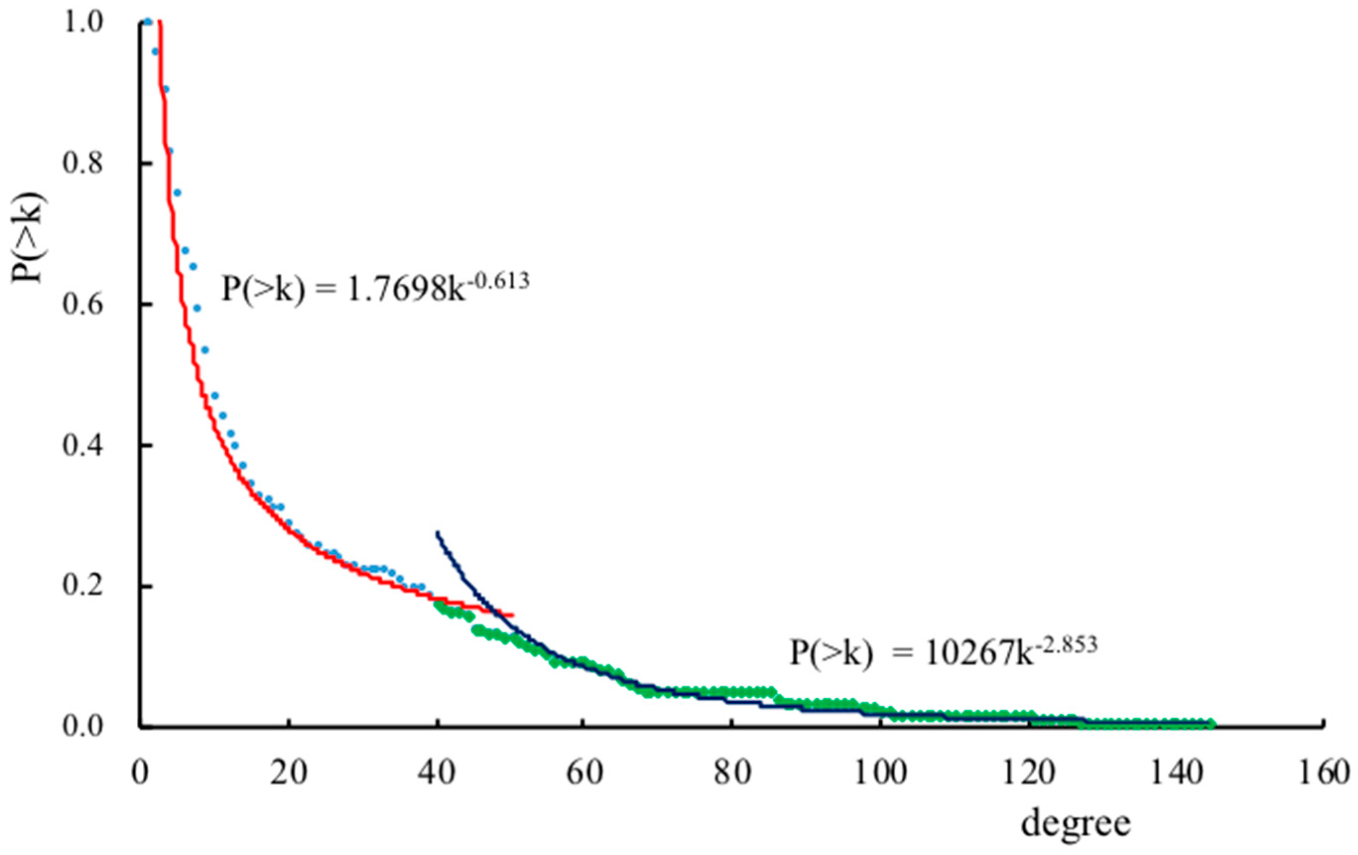
There are some basic indicators of networks, such as the degree ($k$), the average shortest path ($d$), and the clustering coefficient ($C$) [24]. The degree ($k_i$) is the number of edges that a vertex i shares with other vertices. The average degree of a network is the average number of neighbors that each vertex has. The average shortest path of a network is defined as the average number of edges along the shortest paths for all of its possible vertex-pairs. The clustering coefficient (c_i) of a vertex i is defined as the ratio of the number of edges that it shares with its neighboring vertices, up to the maximum possible number. For a network with n vertices, if n_k of them have a degree of k, the degree distribution (denoted as (k)) is defined as the fraction of these k-degree vertices, i.e., n_k/n. (>k) represents the cumulative degree distribution, i.e., the fraction of vertices with degrees that are greater than or equal to k. The distribution of degrees of a network is an important feature that reflects the network topology, and it indicates the process by which the network comes into existence. A random network shows a Poisson (exponential) connectivity distribution ((k)). For a scale-free network, (k) decays as a power law (i.e., (k)~k^−γ).

2.1.2. Clustering

Considering the effect of weights (i.e., the available passenger-seats assigned to the respective edge), we can attain better insights into the structural properties of the CAPN. By extending the clustering coefficient definition, the weighted clustering coefficient is defined as:

$$c_i^w=\frac{1}{s_i\left(k_i-1\right)}{\displaystyle \sum _{j,h}\frac{\left(w_{ij}+w_{ih}\right)}{2}{a}_{ij}{a}_{ih}{a}_{jh}}$$

(1)

where $s_i$ is the strength of vertex $i$, which is the total weight of its edges.

The weighted clustering coefficient is a measure of the local cohesiveness that takes into account the importance of the clustered structure on the basis of the amount of weight that is actually found on the local cluster [8]. The number of clusters in the neighborhood of a vertex is considered, and the total relative weight of the edges is also considered. Generally, there are two opposite cases. If the weighted clustering coefficient is larger than the clustering coefficient, it is inferred that in the network, the interconnected clusters are more likely formed by the edges with larger weights. On the other hand, the weighted clustering coefficient, being smaller than the clustering coefficient, displays a network in which the topological clusters are generated by the edges with low weights, and the clusters have a minor effect on the organization of the network, because the largest part of the flow occurs on edges that do not belong to the interconnected clusters.

2.1.3. Assortative Mixing

In a network, the connection of vertices may imply a tendency where high-degree vertices prefer to attach to other high-degree vertices, which is called assortative mixing or low-degree vertices in a disassortative mixing mode. The average nearest-neighbors degree for vertices with degree k, denoted as $k_{nn}$, provides a way to probe such properties of networks. If $k_{nn}\left(k\right)$ is an increasing function of k, vertices with a high degree have larger probabilities of being connected with high-degree vertices. In contrast, a decreasing behavior of $k_{nn}\left(k\right)$ reflects disassortative mixing, in the sense that high-degree vertices have a majority of neighbors with low degrees. The weighted average nearest-neighbors degree is defined as [8]:

$$k_{nn}^w=\frac{1}{s_i}{\displaystyle \sum _j{a}_{ij}{w}_{ij}{k}_j}$$

(2)

This definition combines the effect of the degree and the weight, and it measures the affinity of vertices to connect to high-degree or low-degree neighbors, depending on the edge weights. If $k_{nn}^w>k_{nn}$, the edges with larger weights are linking the neighbors with higher degrees; while $k_{nn}^w<k_{nn}$ in the opposite case.

To better describe the assortativity, the assortativity coefficient (r) is defined as:

$$r=\frac{M^{-1}{\displaystyle \sum a_{ij}{k}_i{k}_j}-{\left[M^{-1}{\displaystyle \sum \frac{1}{2}{a}_{ij}\left(k_i+k_j\right)}\right]}^2}{M^{-1}{\displaystyle \sum \frac{1}{2}{a}_{ij}\left(k_i^2+k_j^2\right)}-{\left[M^{-1}{\displaystyle \sum \frac{1}{2}{a}_{ij}\left(k_i+k_j\right)}\right]}^2}$$

(3)

where $M$ is the total number of edges in the network.

The assortativity coefficient formula extends from the Pearson correlation coefficient of the degrees at either ends of an edge [25]. The value $r$ of a network is in the range [−1, 1], where it is positive for assortative mixing and negative for disassortative mixing. The value $\left|r\right|$ indicates the intention. Besides, the weighted assortativity coefficient is put forward to let the weights of edges make sense.

$$r^w=\frac{H^{-1}{\displaystyle \sum w_{ij}{k}_i{k}_j}-{\left[H^{-1}{\displaystyle \sum \frac{1}{2}{w}_{ij}\left(k_i+k_j\right)}\right]}^2}{H^{-1}{\displaystyle \sum \frac{1}{2}{w}_{ij}\left(k_i^2+k_j^2\right)}-{\left[H^{-1}{\displaystyle \sum \frac{1}{2}{w}_{ij}\left(k_i+k_j\right)}\right]}^2}$$

(4)

where $H$ is the total strength of vertices in the network.

2.1.4. Centrality

Apart from the topological properties of whole networks, some important vertices may remarkably affect networks. Networks are formed by the interconnection, and the vertex cannot work itself, so the influence of vertices on each other should be a concern. Important vertices can be identified through the concept of centrality, which can be quantified by various indicators. We choose the following four indicators to describe the centrality property of the CAPN.

(i) The degree is the most basic and simple for measuring the importance of vertices, and the degree centrality is defined as:

$$C_D\left(i\right)=\frac{k_i}{N-1}$$

(5)

where $N$ is the total number of vertices in the network and $C_D\left(i\right)$ is a normalized value conveying the ability that a vertex can interact directly with other vertices.

(ii) All pairs of vertices have a distance in connected networks. For a vertex $i$, the reciprocal of the sum of its shortest path from all other vertices is defined as the closeness centrality [26], i.e.:

$$C_C\left(i\right)=\frac{N-1}{{\displaystyle \sum _{j=1,j\ne i}^{N}d\left(i,j\right)}}$$

(6)

The closeness centrality measures the accessibility of vertices, and it reveals the average level of communication between vertices. Because of the reciprocal, the more central a vertex is, the lower its total distance from all other vertices, i.e., the larger the closeness centrality is.

(iii) The times in which a vertex participates in shortest paths reflect the importance of the vertex in the network. It is possible to quantify the importance of a vertex in terms of its betweenness centrality, i.e.:

$$C_B\left(i\right)={\displaystyle \sum _{jk}\frac{\sigma \left(j,i,k\right)}{\sigma \left(j,k\right)}}$$

(7)

where $\sigma \left(j,i,k\right)$ is the number of shortest paths between vertices $j$ and $k$ that pass through vertex $i$ and $\sigma \left(j,k\right)$ is the total number of shortest paths between $j$ and $k$. A vertex involved in more shortest-paths is usually more important, and the betweenness centrality is used to quantify a vertex’s importance as an intermediary.

(iv) A network can be represented in the matrix way. For the adjacency matrix $A$, the vector-matrix notation is $Ax=\lambda x$, where $\lambda$ is the largest eigenvalue and $x=\left(x_1,x_2,\cdots ,x_n\right)$ is the associated eigenvector. A vertex’s centrality should depend on the centrality of its neighbors topologically, with the edges with larger weights indicating higher centrality. The weighted eigenvector centrality [27] is defined as:

$$C_E^w\left(i\right)=\frac{1}{\lambda }{\displaystyle \sum _{j=1}^N{a}_{ij}{w}_{ij}{x}_j}$$

(8)

2.1.5. Rich-Club

Networks involve the interaction between vertices, and this tendency is observed in many real networks in that large vertices are always well-connected with each other. This phenomenon, known as the rich-club, is usually measured by the rich-club coefficient that determines how the large vertices work together [28]. The rich-club coefficient gives the fraction of existing edges among vertices with degrees that are larger than $k$. The rich-club coefficient is defined as:

$$\varphi \left(k\right)=\frac{1}{\left|R\left(k\right)\right|\left(\left|R\left(k\right)\right|-1\right)}{\displaystyle \sum _{i,j\in R\left(k\right)}{a}_{ij}}$$

(9)

where $R\left(k\right)$ is the set of rich vertices. The constitution of $R\left(k\right)$ is different when the focused degree $k$ is different. Networks that have high rich-club coefficients are said to establish more edges among the members of the rich-club, and to demonstrate the rich-club effect.

The rich-club coefficient only describes the properties of rich vertices, and it is not a statistical average over the whole network. The weighted rich-club coefficient measures the fraction of weights that are shared by the rich vertices to see if they are connected through the strongest edges of the network. The weighted rich-club coefficient can evaluate whether vertices that are prominent also tend to interchange among themselves the majority of the weight within the network [29]. The weighted rich-club coefficient is defined as:

$${\varphi }^w\left(k\right)=\frac{{\displaystyle \sum _{i,j\in R\left(k\right)}{w}_{ij}}}{{\displaystyle \sum _{n=1}^{\left|E_{R\left(k\right)}\right|}{w}_n^{rank}}}$$

(10)

where $E_{R\left(k\right)}$ is the set of edges connecting the members in the rich-club, $w_n^{rank}$ is the ranking of weights for all of the edges in the network, and the denominator is the sum of the strongest edges with the same amount in $E_{R\left(k\right)}$.

2.2. The Non-parametric Spectral Destiny Estimation with a Window Function

The spectral destiny estimation, which is usually used to analyze the cycle in economic indicators, is used to estimate the spectral density of the sample from a time sequence, and one of its purposes is the detection of periodicities in the data, by observing peaks in the frequencies [30]. There are many concrete ways to conduct spectral destiny estimation in the literature. We choose the non-parametric spectral destiny estimation with a window function to find the cycles in CAPN subnet indicators. The window function is a mathematical function that is zero-valued outside of some fixed intervals, and its impact is to reduce the spectral leakage [31].

In Section 2.2, the parameters $M$ and $N$ have different meanings compared with those in Section 2.1. Choosing the width of window $M$ is a key problem in implementing the spectral destiny estimation with a window function, while $M$ should be neither too large nor too small [32]. To ensure the ability to distinguish between spectral peaks, $2\sqrt{N}$ is taken as the value of $M$ in this paper, where $N$ is the sample size. Besides, the frequencies (denoted as $f_j$) with the same interval in the range of the sample are usually selected, and we let $f_j=j/\left(2L\right)$ ($j=0,1,\dots ,L$, where $L$ is the integer part of $N/2$). The estimated value of the spectral density at frequency $f_j$ is:

$$\widehat{h}\left(f_j\right)={\displaystyle \sum _{k=-M}^{M}w\left(k\right)\widehat{R}\left(k\right)\cos \left(2\pi f_{j}k\right)}=2R\left(0\right)+2{\displaystyle \sum _{k=1}^{M}w\left(k\right)\widehat{R}\left(k\right)\cos \left(2\pi f_{j}k\right)}$$

(11)

where $\widehat{R}\left(k\right)$ is the autocovariance function of samples:

$$\widehat{R}\left(k\right)=\frac{1}{N}{\displaystyle \sum _{t=1}^{N-k}\left(x_t-\overline{x}\right)\left(x_{t+k}-\overline{x}\right)}\left(k=0,1,\dots ,M\right)$$

(12)

$\overline{x}$ is the sample average:

$$\overline{x}=\frac{1}{N}{\displaystyle \sum _{t=1}^N{x}_t}$$

(13)

and $w\left(k\right)$ is the window function. The Tukey-Hanning window is selected here, and $w\left(k\right)$ is defined as:

$$w\left(k\right)=\{\begin{array}{l}\frac{1}{2}\left(1+\cos \frac{\pi k}{M}\right),\left|k\right|\le M\\ 0,\left|k\right|>M\end{array}$$

(14)

Generally, there are some peaks in the sequence of estimated values, but one cannot immediately determine whether the corresponding frequencies are the real cycles in the value sequence. A statistical test is necessary to check the cycle. For the results of the spectral destiny estimation, let $I_{\left(P\right)}$ be the value of the p-th peak. The ratio $g_{\left(P\right)}=I_{\left(P\right)}/{\displaystyle \sum I_{\left(P\right)}}$ can be calculated, where the denominator is the sum of the values of all peaks. [33] Deduced the probability distribution of $g_{\left(P\right)}$ under the assumption that there are no cycles in the sequence. By using this distribution, the assumption can be tested for the p-th peak. To a given confidence level $\alpha$, if $g_{\left(P\right)}<z_{\alpha }$ where $z_{\alpha }$ is from the significance test table according to $p$ and $L$, the assumption is refused and the cycle is true. If the test shows that the first peak is significant, the other peaks are tested one by one.

3. Results

3.1. The Structural Features of the CAPN

(i) In the CAPN, for an airport, $k$ is the number of directly-connected airports, $d$ is the average minimum number of airlines that one needs to take to get from an airport to another airport, and $C$ is the probability that two airports that are directly connected to the same airport are also directly connected to each other. These basic indicators can convey two common properties of real networks as the CAPN.

One is the small-world property, as indicated by a high clustering coefficient and a small average shortest path.

Table 1. Some basic properties of several types of air transportation networks.

Network Type	Vertex Number	$\mathit{d}$	$\mathit{C}$
World Wide [11]	3883	4.40	0.62
World Wide [32]	3712	3.94	0.64
Europe [33]	601	4.04	0.62
The U.S. [18]	272	1.84~1.93	0.73~0.78
Brazil [21]	142	2.34	0.63
Australia [34]	131	2.90	0.50
India [1]	79	2.26	0.66
China [15]	144	2.23	0.69
China [17]	140	2.11	0.74
The CAPN in this paper	174	1.98	0.80

compares the topological properties of the CAPN with those of other types of air transportation networks. The clustering coefficient (C = 0.80) is slightly larger than those of other types of air transportation networks. The average shortest path length (d) of the CAPN is 1.98, which indicates that, on average, about two flight changes are required to connect most airport-pairs. The average shortest path length of the CAPN is similar to those of India [1], Brazil [21], and the U.S. [18], but much less than that of the world [11,32]. It can be inferred that the CAPN evolves as a small-world topology, which means that it is possible to fly from one airport to another through a small number of intermediate airports. All of the network features presented in Table 1 imply that the CAPN has properties that are similar to small-world characteristics.

The other is the scale-free property, which is characterized by a power-law $P\left(k\right)\sim k^{-\gamma }$. The cumulative degree distribution ((>k)) of the CAPN is analyzed manually and illustrated in Figure 1, in which it can be seen that a two-regime power-law distribution is followed. It is confirmed that a small number of airports carry the majority of the airlines. This scale-free structure could be robust for a random failure, but vulnerable to a targeted or specific failure.

(ii) The weighted clustering coefficient of the CAPN is 0.85, which is larger than the clustering coefficient of the CAPN (i.e., 0.80). This statistical result reflects that the airports are connected closely, and that the large passenger capacities take part in the formation of clusters on that basis.

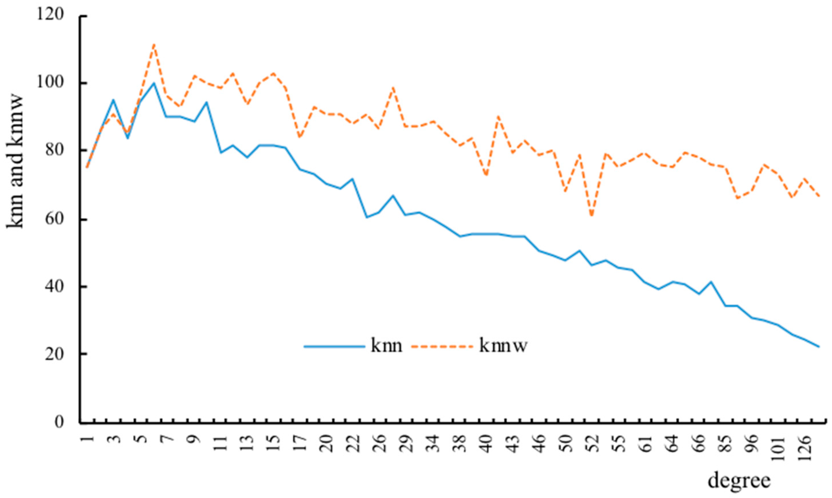
(iii) Figure 2 shows the result that the higher the degrees that the vertices have, the lower the degrees that their neighbors have on the CAPN. This result implies that the CAPN tends to be disassortative. National hubs or large airports are required to provide connectivity to a large number of low-degree destinations. Concluded by $k_{nn}^w>k_{nn}$, the passenger capacities are assigned between high-degree vertices.

The weighted assortativity coefficient (i.e., $r^w$) better describes the assortativity of networks with weighted edges. If $r^w>r$, a high-weighted edge tends to connect two similar degree vertices; otherwise, the degree of vertices connected by high-weighted edges may have large differences [35]. The value of $r$ is −0.53, and for $r^w$, it is −0.17 for the CAPN. This indicates that large passenger capacities exist between large airports on the CAPN when considering the results of $k_{nn}^w>k_{nn}$ and $r^w>r$.

(iv) In

Table 2. Top 15 airports of the CAPN under different centrality indicators.

Rank	Degree Centrality		Closeness Centrality		Betweenness Centrality		Weighted Eigenvector Centrality
	City	Value	City	Value	City	Value	City	Value
1	Beijing	0.83237	Beijing	0.85222	Beijing	0.20603	Shanghai	0.42514
2	Shanghai	0.72832	Shanghai	0.78281	Shanghai	0.12736	Beijing	0.40838
3	Guangzhou	0.69364	Guangzhou	0.76211	Guangzhou	0.09018	Guangzhou	0.31996
4	Shenzhen	0.58382	Shenzhen	0.70325	Xi’an	0.08615	Shenzhen	0.26692
5	Chengdu	0.57225	Chengdu	0.69758	Chengdu	0.06581	Chengdu	0.25806
6	Xi’an	0.55491	Xi’an	0.69200	Urumqi	0.05434	Xiamen	0.23054
7	Kunming	0.49711	Kunming	0.66284	Shenzhen	0.05399	Kunming	0.22084
8	Xiamen	0.49133	Xiamen	0.65779	Chongqing	0.04759	Chongqing	0.21798
9	Chongqing	0.49133	Chongqing	0.65779	Kunming	0.03663	Xi’an	0.17831
10	Changsha	0.38728	Changsha	0.61786	Xiamen	0.02765	Hangzhou	0.13796
11	Hangzhou	0.38150	Hangzhou	0.61348	Hohhot	0.01739	Wuhan	0.12959
12	Shenyang	0.37572	Shenyang	0.61348	Tianjin	0.01637	Nanjing	0.12732
13	Dalian	0.36994	Dalian	0.61131	Dalian	0.01621	Guiyang	0.12686
14	Haikou	0.36994	Haikou	0.61131	Harbin	0.01485	Qingdao	0.12451
15	Tianjin	0.36416	Tianjin	0.60915	Hangzhou	0.01400	Harbin	0.12202

, we list the top 15 airports. The most central vertices on the CAPN are identified by the four centrality indicators. Generally speaking, the airports located in larger cities always have more central positions, such as Beijing, Shanghai, Guangzhou, Shenzhen, Chengdu, Xi’an, etc. These airports usually act as the national air-hubs. What is the most different is the ranking of the betweenness centrality. The betweenness centrality measures the importance of a vertex in connecting the others, and the airports with key positions between others have high rankings.

Besides the national air-hubs located in larger cities, some airports that may act as local air-hubs; for example, Urumqi, Hohhot, Kunming, Guiyang, Lhasa, etc., also have high rankings. In practice, regional airline networks are constructed in some borderline provinces of China, in which airports located in the provincial capitals are the local air-hubs and the local airlines constitute the edges. The regional networks make the local air-hubs hold important positions in the whole CAPN.

(v) In the CAPN, the first 35 vertices with degrees larger than 35 (i.e., $k>35$) are chosen as the rich-club. The rich-club coefficient is 0.93, which indicates that there are direct airlines between the majority of airports with large degrees. The weighted rich-club coefficient is 0.88, which means that close to 90% of large capacities exist between airports with large degrees. The behavior of the rich vertices in the CAPN implies that rich vertices are closely connected with each other, and that the passenger capacities among them are dominant.

3.2. The Temporal Features of the CAPN Subnets

We investigate the temporal features of the CAPN by certain subnets. To analyze the CAPN more microcosmically, the time-scale interval constraint for extracting subnets is per day or every two-hours, since the collected flight information includes some details. The first type of subnets, named SDD in this paper, was extracted by taking every day in a week as the time-scale interval. The SDD consists of seven networks; each of which is modelled by referring to the data on all flights on each day of a week. The second type of subnets, named SDT in this paper, was extracted by taking two hours as the time-scale interval. On every day in a week, the time from 6:00 a.m. to 10:00 p.m. was considered, while other time intervals with not enough flights are excluded. For an airport, any flights with departure times in the corresponding two-hour interval are considered. Within the two-hour interval, the SDT consists of 56 networks with a time range from 6:00 a.m. on Monday to 10:00 p.m. on Sunday.

3.2.1. The SDD Network

The number of vertices in every SDD network is almost the same as that in the CAPN, while the edges of every SDD network are obviously less than those of the CAPN. In official schedules, some flights between two airports are scheduled every two-days, which leads to different numbers of edges on each day of a week. The indicator results show that the features have no particular difference among the seven SDD networks, and between the seven SDD networks and the CAPN (see

Table 3. Results of indicators of the first type of subnets (SDD).

	Mon.	Tue.	Wed.	Thu.	Fri.	Sat.	Sun.	CAPN
Vertices	171	172	171	172	172	172	171	174
Edges	1525	1529	1547	1521	1541	1524	1538	1787
$C$	0.806	0.778	0.800	0.774	0.792	0.778	0.792	0.795
$C^w$	0.852	0.822	0.846	0.820	0.837	0.823	0.838	0.848
$d$	2.025	2.032	2.040	2.040	2.044	2.031	2.025	1.984
$r$	−0.510	−0.523	−0.511	−0.522	−0.509	−0.519	−0.515	−0.527
$r^w$	−0.175	−0.178	−0.174	−0.170	−0.171	−0.170	−0.177	−0.170
$\varphi \left(k\right)$	0.911	0.909	0.923	0.909	0.918	0.909	0.919	0.930
${\varphi }^w\left(k\right)$	0.879	0.881	0.879	0.883	0.884	0.884	0.882	0.876

). The SDD network has small-world, disassortative mixing, and rich-club properties. Some properties of subnets of different days have slight fluctuations. Probable reasons for this are summarized as follows. Firstly, there is usually more than one flight between two airports, and the two airports are still linked, although some flights have been eliminated by the time interval constraint. Secondly, some of the feeder airports and flights are filtered out by the time interval constraint for the reduction of vertices and edges, which occurs alternately on different days. The absence of some of airports and flights does not happen on the same day. On the whole, the numerical values of some indicators of the SDD networks remain relatively stable.

3.2.2. The SDT Network

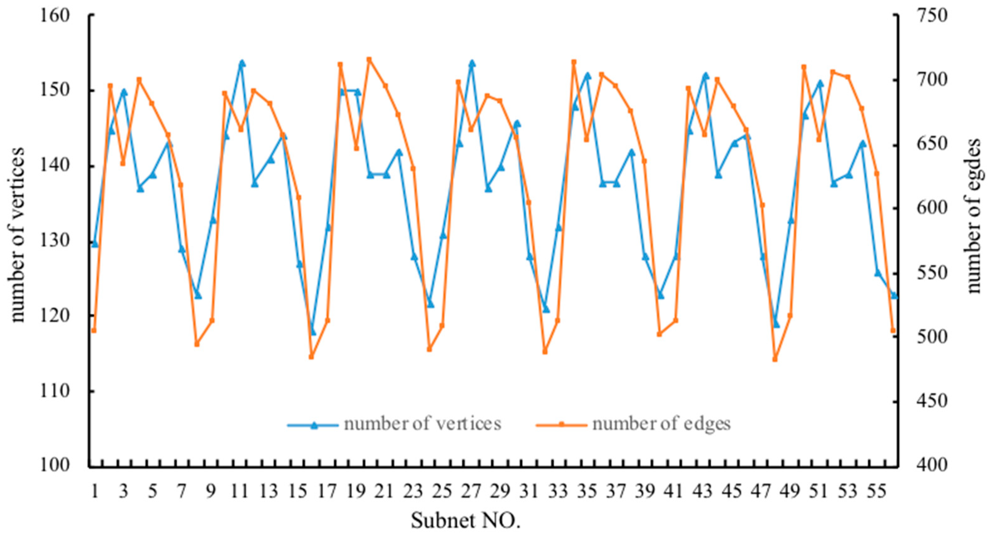
SDT network properties may shed light on the air network performance and the changing rule more accurately and microcosmically in the course of all periods of every day. Corresponding to the eight two-hour intervals of each day in a week, the 56 SDT networks are numbered from 1 to 56. As is shown in Figure 3, any one of the SDT networks is smaller than the CAPN in the numbers of included vertices and edges. The maximum number of edges of SDT networks is 716, which is even less than half of the CAPN edges. The scales of 56 SDT networks imply an obvious periodicity tendency. On each day, the departure time of the majority of flights is from 10:00 a.m. to 12:00 a.m., and most airports are involved at the time from 8:00 a.m. to 10:00 a.m., and from 12:00 a.m. to 2:00 p.m. However, in this situation, the peak numbers of the involved airports and flights do not appear in the same time interval. The possible reason for this is that more feeder airports that have few scheduled flights take part in the network from 10:00 a.m. to 12:00 a.m.; e.g., the remote airports in Yushu, Altay, and Korla, and tourist airports in Jingdezhen, Jiuzhaigou, and Dunhuang only have one or two flights from 10:00 a.m. to 12:00 a.m.

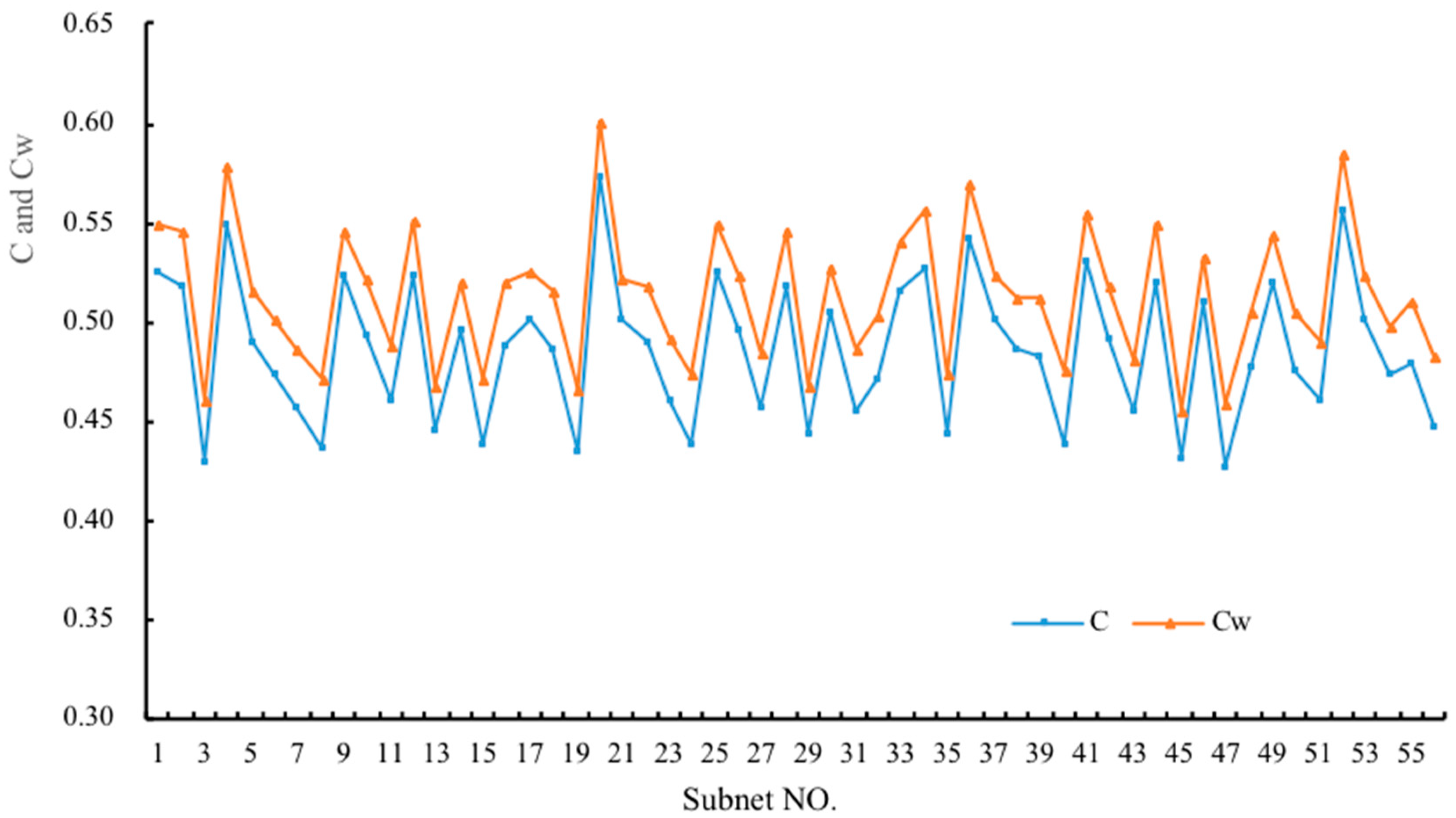
Including a smaller number of edges, the properties of SDT networks change a little, compared to the CAPN. The CAPN obviously has a small-world property. When it comes to SDT networks, the average clustering coefficient is only 0.49, and the average short path is 2.39, which manifests that the small-world property is weakened, together with the outcome that the average degree is 9.14 for the SDT networks, which is far less than that of the CAPN (i.e., 20.54). There is no sufficient direct connection between airports in SDT networks, which leads to difficult transportation. The property that the weighted clustering coefficients are always larger than the clustering coefficients is kept still, which can be found from Figure 4. Including those limited by less edges, not so many clusters are formed in SDT networks. The edges with higher weight are much more likely to form clusters and large-capacity airlines still play an important role between airports such as Beijing, Shanghai, and Guangzhou, where passenger capacities on the airline always have the top rankings in all SDT networks.

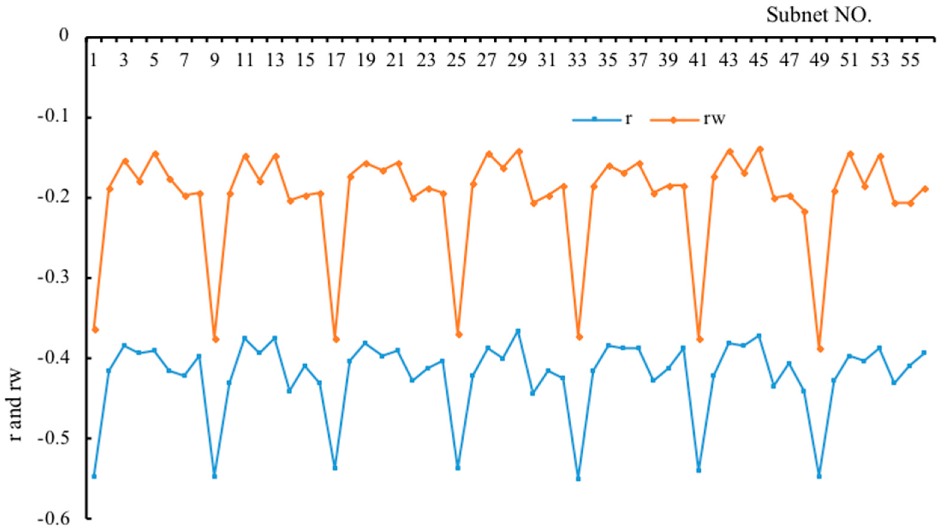
The SDT also has the property that $k_{nn}^w$ is larger than $k_{nn}$. An edge with a large passenger capacity will always want to link the vertices with large degrees. This is easy to understand, since more flights will be scheduled between the airports that are large enough, and provide transportation services for large cities. Besides, some flights from large airports will connect other airports at small scales to maintain the connectivity and flexibility of the whole air network. As a result, the SDT networks become disassortative. $k_{nn}$ decreases along with the degree increase, and so does the $k_{nn}^w$. This indicates that the larger degree that a vertex has, the smaller the average degree that its neighbor vertices have, which is in accordance with how the disassortative networks perform. The disassortative property reflects the tendency that large degree airports link many small degree airports to enhance the total passenger demand in a cost-effective and infrastructure-efficient design [18]. This tendency is described quantitatively by using the assortativity coefficient. The assortativity coefficient of the SDT networks is negative, and it seems periodical. The average assortativity coefficient is −0.42, and the average weighted assortativity coefficient is −0.20, which indicate the type of disassortative networks. The time interval from 6:00 a.m. to 8:00 a.m. is the most disassortative. It is speculated that large airports may operate earlier to connect other airports, while many airports do not have scheduled flights between each other from 6:00 a.m. to 8:00 a.m. The property that $r^w$ is larger than $r$ is maintained (see Figure 5), conveying that in SDT networks, the large capacity is likely to exist between airports with similar scales. Large airports ensure the dominant position by controlling the flow.

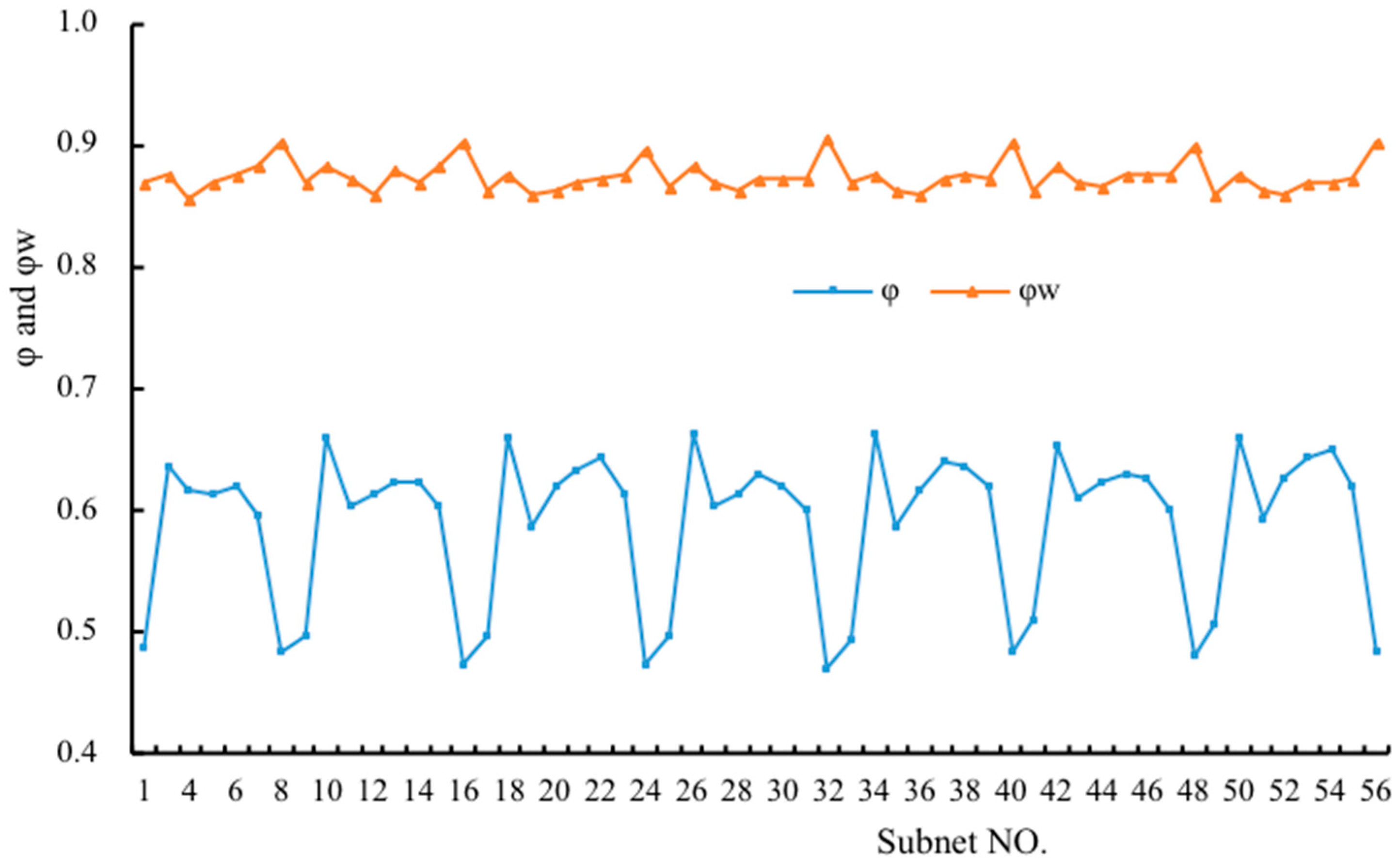
For the rankings of centrality, all of the rankings of SDT networks show a similar structure that is in accordance with the result that the CAPN shows. There are two types of airports at the top of the rankings. The first are those located in large cities with relatively-well-developed economies and societies. The second are those that act as local hubs, providing powerful bridges. It is costly and unnecessary to make all airports directly connect. In local regions, there are some feeder airports whose flights are few and they only connect with each other and their local hub. Generally, these two types of airports are more significant in the extracted subnets. There is no obvious change in the rankings of the important vertices. The average rich-club coefficient of all SDT networks is 0.59, which is obviously smaller than that of the CAPN. It indicates that over half of the connections between most airports with large degrees are linked by direct flights. A periodic property is implied in the rich-club coefficient results. The rich-club coefficient is small at the beginning and at the end of a day, and it is large in the period from 8:00 a.m. to 10:00 a.m. (see Figure 6). Though rich-club members are not closely connected, the weighted rich-club coefficient with an average value 0.87 is relatively large, and there is no particular fluctuation in the weighted rich-club coefficient results. The passenger capacity of the rich-club is dominant in SDT networks, and the important airports usually sustain high flow volumes.

3.3. The Periodicity of the CAPN Subnets

Several of the CAPN subnet features imply certain periodic properties, and specific conclusions are attained from an experiential perspective. It is worth exploring further whether the indicators of the CAPN subnets have implicit cycles. We employ here the method of the spectral destiny estimation to mathematically find the implicit periodicity.

Table 4. The spectral-destiny-estimation results of SDT network indicators (confidence level $\alpha =0.01$).

Indicators	p-th Peak	Possible Cycle	${\mathit{z}}_{0.01}$	$\mathit{g}\left(\mathit{r}\right)$	Indicators	p-th Peak	Possible Cycle	${\mathit{z}}_{0.01}$	$\mathit{g}\left(\mathit{r}\right)$
Number of Vertices	1st	8	0.256	0.087	$K_{nn}^w$	1st	15	0.256	0.070
	2nd	15	0.162	0.057		2nd	8	0.162	0.053
Number of Edges	1st	8	0.256	0.093		3rd	22	0.138	0.044
	2nd	15	0.162	0.039	$r$	1st	8	0.256	0.062
	3rd	22	0.138	0.032		2nd	22	0.162	0.054
$\langle k\rangle$	1st	8	0.256	0.074		3rd	15	0.138	0.045
	2nd	22	0.162	0.062	$r^w$	1st	8	0.256	0.063
$C$	1st	22	0.256	0.062		2nd	22	0.162	0.056
	2nd	15	0.162	0.041		3rd	15	0.138	0.042
$C^w$	1st	22	0.256	0.063	$\varphi \left(k\right)$	1st	8	0.256	0.070
	2nd	15	0.162	0.037		2nd	15	0.162	0.058
$K_{nn}$	1st	15	0.256	0.077		3rd	22	0.138	0.038
	2nd	22	0.162	0.044	${\varphi }^w\left(k\right)$	1st	8	0.256	0.063
	3rd	8	0.138	0.044		2nd	22	0.162	0.061

shows the estimation results and the test results for the SDT network indicators. At the confidence level of $\alpha =0.01$, any $g_{\left(P\right)}$ is not larger than $z_{\alpha }$. It is concluded that the peaks shown in

Table 5. The frequency and schedule mode of flights in a week.

Frequency	Flights		Schedule Mode	Flights
	Number	Percentage		Number	Percentage
7	12709	59.0	1111111	12709	59.0
6	1004	4.7	0101010	1310	6.1
5	781	3.6	1010101	1238	5.7
4	2029	9.4	0010101	276	1.3
3	2674	12.4	1010100	237	1.1
2	1012	4.7	0101011	169	0.8
1	1343	6.2	Other modes	5613	26.0

Note: A binary sequence is used to represent the schedule mode of flights from Monday to Sunday. If one flight is scheduled on Monday, the first number of the sequence is 1; otherwise, it is 0. The rest of the numbers can be done in the same manner. As a whole, all 127 types of schedule modes except all zeroes appear in the flight schedules.

are not false, and that all of the implicit cycles are true.

The periodicity of the CAPN subnets is summarized as follows.

(i) For each indicator of SDT networks, there exists an obviously significant cycle that corresponds to the first peak in the sequence of estimated values. For most indicators, the first cycle is 8, which means that a cycle of one natural day is common. Considering the flight schedules (Table 5), 59% of flights fly every day, and other flights may be absent over some days. The schedule mode of flights in a week indicates that most flights are scheduled with one day as the interval, which contributes to one day as the first cycle.

(ii) Besides the one-day cycle, there are another two types of cycles that can be found by the spectral destiny estimation method; i.e., 15 and 22, which correspond to about two and three days, respectively. Based on schedule modes such as “0101010” and “1010101” in flight schedules (as shown in Table 5), a cycle of two days can also have an effect. Moreover, there is still quite a large proportion of flights that are scheduled by other schedule modes. The spectral density estimation computation reveals that a three-day cycle can be found.

(iii) Compared with the vertices, the edges of the SDT networks are more flexible and changeable. The number and locations of airports are fixed for a long time, while the schedule of flights is relatively flexible, which leads to differences between the SDT networks. The SDT network is the interaction by airports and flights, where the properties shown are affected by the interaction. Although three implicit cycles are found by the spectral destiny estimation method, the numbers of cycles implied by the sample data of different indicators are different. The indicators that involve vertices and passenger capacities on edges, such as the number of vertices, the average degree, and the weighted rich-club coefficient, generally have two cycles. The indicators that involve the quantity and status of connection between vertices, such as the number of edges and the assortativity coefficient, generally have three cycles.

The Chinese air passenger system presently plays a crucial role in people mobility in China. Finding the mechanism that drives air transportation dynamics is a necessary step to better controlling and optimizing the function of the air passenger system. The mechanism involves the periodicity, which reflects the passenger needs being guided by the fluctuant configuration of the air resources. Understanding the periodic mechanism is fundamental for better air network designs that benefit airlines and passengers.

4. Conclusions

The complex network theory has helped the research community to investigate various air networks’ structures and properties. As a case study, this paper aimed to analyze the Chinese air passenger network (CAPN) from holistic and more microcosmic perspectives. The topological structure of an air network obviously has impacts on the network’s performance, and the capacity (e.g., available passenger-seats) flow through the structure is also an important indicator, since the capacity induces profits and passengers’ travelling behaviors. The CAPN structure features from the non-weighted and the weighted perspectives are described. Two types of subnets extracted by time-scale constraints of one day or every two-hours are used to find the temporal features. The spectral destiny estimation method is used to find the implicit periodicity mathematically, since the CAPN subnet features seem to imply some periodic properties.

The results indicate that the CAPN has a small-world and scale-free structure. The clustering coefficient (i.e., 0.80) is relatively large. The average shortest path length is 1.98, which is similar to those of India, Brazil, and the U.S., but much less than that of the world. The cumulative degree distribution follows a two-regime power-law distribution, which confirms that a small number of airports carry the majority of the flights. The weighted clustering coefficient (i.e., 0.85) is larger than the clustering coefficient (i.e., 0.80), which reflects that the airports are closely connected, and the large capacities take part in the formation of clusters on that basis. The CAPN tends to be disassortative. National hubs or large airports are required to provide connectivity to a large number of low-degree destinations. Large capacities exist between large airports. Apart from the topological properties of whole networks, some important airports, including national air-hubs and local air-hubs, remarkably affect the CAPN. About 90% of large capacities exist between airports with large degrees. Rich vertices are closely connected with each other, and the passenger capacities among them are dominant.

The properties of CAPN subnets extracted by taking two hours as the time-scale interval (i.e., SDT networks) shed light on the air network performance and the changing rule more accurately and microcosmically. For SDT networks, the average clustering coefficient is 0.49, and the average short path is 2.39. Several of the CAPN subnet features imply some periodic property, and the method of the spectral destiny estimation is used to find the implicit periodicity mathematically. For most indicators of SDT networks, a one-day cycle, two-day cycle, and/or three-day cycle can be found. The periodicity mechanism reflects that passenger needs are guided by the fluctuant configuration of air resources. Understanding the periodic mechanism is fundamental to better designing the air network that benefits airlines and passengers.

Our work is based on the adjacency matrix and the weight matrix that represent the CAPN. The matrix data can be attained by emailing the corresponding author. This paper provides some valuable conclusions about the structural characteristics and temporal features of the CAPN, which serve as a baseline for other research. The analysis conclusions offer an insight into the configuration mode of air capacity in the whole CAPN at a macro and industrial level. For future study, the conclusions of this paper may be improved and calibrated by linking the models of firm and passenger behaviors.

References

- Bagler, G. Analysis of the airport network of India as a complex weighted network. Phys. A Stat. Mech. Its Appl. 2008, 387, 2972–2980. [Google Scholar] [CrossRef] [Green Version]
- Lordan, O.; Sallan, J.M.; Simo, P.; Gonzalez-Prieto, D. Robustness of the air transport network. Transp. Res. Part E Logist. Transp. Rev. 2014, 68, 155–163. [Google Scholar] [CrossRef]
- Lin, J.; Ban, Y. The evolving network structure of US airline system during 1990–2010. Phys. A Stat. Mech. Its Appl. 2014, 410, 302–312. [Google Scholar] [CrossRef]
- Zhang, J.; Cao, X.B.; Du, W.B.; Cai, K.Q. Evolution of Chinese airport network. Phys. A Stat. Mech. Its Appl. 2010, 389, 3922–3931. [Google Scholar] [CrossRef] [Green Version]
- Jia, T.; Qin, K.; Shan, J. An exploratory analysis on the evolution of the US airport network. Phys. A Stat. Mech. Its Appl. 2014, 413, 266–279. [Google Scholar] [CrossRef]
- Lordan, O.; Sallan, J.M. Analyzing the multilevel structure of the European airport network. Chin. J. Aeronaut. 2017, 30, 554–560. [Google Scholar] [CrossRef]
- Amaral, L.A.N.; Scala, A.; Barthelemy, M.; Stanley, H.E. Classes of small-world networks. Proc. Natl. Acad. Sci. USA 2000, 97, 11149–11152. [Google Scholar] [CrossRef] [PubMed] [Green Version]
- Barrat, A.; Barthelemy, M.; Pastor-Satorras, R.; Vespignani, A. The architecture of complex weighted networks. Proc. Natl. Acad. Sci. USA 2004, 101, 3747–3752. [Google Scholar] [CrossRef] [Green Version]
- Barrat, A.; Barthélemy, M.; Vespignani, A. The effects of spatial constraints on the evolution of weighted complex networks. J. Stat. Mech. Theory Exp. 2005, 2005, P05003. [Google Scholar] [CrossRef]
- Guimera, R.; Amaral, L.A.N. Modeling the world-wide airport network. Eur. Phys. J. B-Condens. Matter Complex Syst. 2004, 38, 381–385. [Google Scholar] [CrossRef]
- Guimera, R.; Mossa, S.; Turtschi, A.; Amaral, L.N. The worldwide air transportation network: Anomalous centrality, community structure, and cities’ global roles. Proc. Natl. Acad. Sci. USA 2005, 102, 7794–7799. [Google Scholar] [CrossRef] [PubMed]
- Colizza, V.; Barrat, A.; Barthélemy, M.; Vespignani, A. The role of the airline transportation network in the prediction and predictability of global epidemics. Proc. Natl. Acad. Sci. USA 2006, 103, 2015–2020. [Google Scholar] [CrossRef] [PubMed] [Green Version]
- Li, W.; Cai, X. Statistical analysis of airport network of China. Phys. Rev. E 2004, 69, 046106. [Google Scholar] [CrossRef] [PubMed] [Green Version]
- Liu, H.K.; Zhang, X.L.; Zhou, T. Structure and external factors of Chinese city airline network. Phys. Procedia 2010, 3, 1781–1789. [Google Scholar] [CrossRef]
- Wang, J.; Mo, H.; Wang, F.; Jin, F. Exploring the network structure and nodal centrality of China’s air transport network: A complex network approach. J. Transp. Geogr. 2011, 19, 712–721. [Google Scholar] [CrossRef]
- Cai, K.Q.; Zhang, J.; Du, W.B.; Cao, X.B. Analysis of the Chinese air route network as a complex network. Chin. Phys. B 2012, 21, 028903. [Google Scholar] [CrossRef]
- Lin, J. Network analysis of China’s aviation system, statistical and spatial structure. J. Transp. Geogr. 2012, 22, 109–117. [Google Scholar] [CrossRef]
- Xu, Z.; Harriss, R. Exploring the structure of the US intercity passenger air transportation network: A weighted complex network approach. GeoJournal 2008, 73, 87. [Google Scholar] [CrossRef]
- Gautreau, A.; Barrat, A.; Barthélemy, M. Microdynamics in stationary complex networks. Proc. Natl. Acad. Sci. USA 2009, 106, 8847–8852. [Google Scholar] [CrossRef] [Green Version]
- Guida, M.; Maria, F. Topology of the Italian airport network: A scale-free small-world network with a fractal structure? Chaos Solitons Fractals 2007, 31, 527–536. [Google Scholar] [CrossRef]
- Da Rocha, L.E. Structural evolution of the Brazilian airport network. J. Stat. Mech. Theory Exp. 2009, 2009, P04020. [Google Scholar] [CrossRef]
- Wang, J.; Mo, H.; Wang, F. Evolution of air transport network of China 1930–2012. J. Transp. Geogr. 2014, 40, 145–158. [Google Scholar] [CrossRef]
- Rocha, L.E.C. Dynamics of air transport networks: A review from a complex systems perspective. Chin. J. Aeronaut. 2017, 30, 469–478. [Google Scholar] [CrossRef]
- Costa, L.D.F.; Rodrigues, F.A.; Travieso, G.; Villas Boas, P.R. Characterization of complex networks: A survey of measurements. Adv. Phys. 2007, 56, 167–242. [Google Scholar] [CrossRef] [Green Version]
- Newman, M.E. Assortative mixing in networks. Phys. Rev. Lett. 2002, 89, 208701. [Google Scholar] [CrossRef] [PubMed]
- Boccaletti, S.; Latora, V.; Moreno, Y.; Chavez, M.; Hwang, D.U. Complex networks: Structure and dynamics. Phys. Rep. 2006, 424, 175–308. [Google Scholar] [CrossRef] [Green Version]
- Soh, H.; Lim, S.; Zhang, T.; Fu, X.; Lee, G.K.K.; Hung, T.G.G.; Di, P.; Prakasam, S.; Wong, L. Weighted complex network analysis of travel routes on the Singapore public transportation system. Phys. A Stat. Mech. Its Appl. 2010, 389, 5852–5863. [Google Scholar] [CrossRef]
- Xu, X.K.; Zhang, J.; Small, M. Rich-club connectivity dominates assortativity and transitivity of complex networks. Phys. Rev. E 2010, 82, 046117. [Google Scholar] [CrossRef]
- Opsahl, T.; Colizza, V.; Panzarasa, P.; Ramasco, J.J. Prominence and control: The weighted rich-club effect. Phys. Rev. Lett. 2008, 101, 168702. [Google Scholar] [CrossRef]
- Gangopadhyay, A.K.; Mallick, B.K.; Denison, D.G.T. Estimation of spectral density of a stationary time series via an asymptotic representation of the periodogram. J. Stat. Plan. Inference 1999, 75, 281–290. [Google Scholar] [CrossRef]
- Swanson, D.C. Precision spectral peak frequency measurement using a window leakage ratio function. Mech. Syst. Signal Process. 2015, 54–55, 1–15. [Google Scholar] [CrossRef]
- Chen, Q.; van Dam, T.; Sneeuw, N.; Collilieux, X.; Weigelt, M.; Rebischung, P. Singular spectrum analysis for modeling seasonal signals from GPS time series. J. Geodyn. 2013, 72, 25–35. [Google Scholar] [CrossRef]
- Grenander, U.; Rosenblatt, M. Statistical Analysis of Stationary Time Series; American Mathematical Soc.: Providence, RI, USA, 2008; Volume 320. [Google Scholar]
- Hossain, M.M.; Alam, S. A complex network approach towards modeling and analysis of the Australian Airport Network. J. Air Transp. Manag. 2017, 60, 1–9. [Google Scholar] [CrossRef]
- Leung, C.C.; Chau, H.F. Weighted assortative and disassortative networks model. Phys. A Stat. Mech. Its Appl. 2007, 378, 591–602. [Google Scholar] [CrossRef] [Green Version]
Figure 1.
The cumulative degree distribution.
Figure 2.
The tendency of (denoted as “knn” in the figure) or (denoted as “knnw” in the figure), along with degrees.
Figure 3.
The scale of the second type of subnets (SDT).
Figure 4.
The clustering coefficient (denoted as “C” in the figure) and the weighted clustering coefficient (denoted as “Cw” in the figure) of SDT networks.
Figure 5.
The assortativity coefficient (denoted as “r” in the figure) and weighted assortativity coefficient (denoted as “rw” in the figure) of SDT networks.
Figure 6.
The rich-club coefficient (denoted as “φ” in the figure) and weighted rich-club coefficient (denoted as “φw” in the figure) of SDT networks.