Ground Deformation Analysis Using InSAR and Backpropagation Prediction with Influencing Factors in Erhai Region, China

Abstract

The long continuity of Interferometric Synthetic Aperture Radar (InSAR) can provide high space and resolution data for ground deformation investigations. The ground deformation in this paper appeared in the city’s development, although it is close to the Erhai region, which is different from a water-deficient city. Therefore, the analysis and prediction of ground deformation using a new method is required. In this study, Sentinel-1 Synthetic Aperture Radar (SAR) images from 2015 to 2018 were used to study the characteristics of ground deformation in the Erhai region using the Small Baseline Subset Interferometric SAR (SBAS-InSAR) technique. The results were cross-validated using ascending and descending direction images to ensure the accuracy. In addition, the results showed that there was little ground deformation in the northern part of the Erhai region, while there was obvious ground deformation in the southern part. Four influencing factors—including the building area, water level, cumulative precipitation, and cumulative temperature of the southern Erhai region—were used together to predict the cumulative ground deformation using back-propagation (BP). The R of all the involved data was 0.966, and the root mean square errors (RMSEs) between the simulated values using BP and the true measured values were 3.063, 1.003, and 1.119, respectively. The results showed that BP has great potential in predicting the change tendency of ground deformation with high precision. The main reason for ground deformation is the continuous increase of building area; the water level followed. The cumulative precipitation and cumulative temperature are the reasons for the seasonal ground deformation. Some countermeasures and suggestions are given to face the challenge of serious ground deformation.

1. Introduction

Ground deformation is defined as the Earth’s surface movement (gradual settling, sudden sinking, or uplift) due to the subsurface movement of Earth materials, which has become a common geological hazard that has caused potential threats to public safety, bringing about a series of harmful impacts [1,2,3,4]. The ground deformation associated with horizontal deformation and the occurrence of ground failures is induced by natural or anthropogenic factors such as underground water withdrawal, long-term drought, and urban construction; however, their causes are puzzles worldwide [5]. Generally, the ground deformation caused by underground water withdrawal has been reported around the world; however, the ground deformations induced by artificial buildings are seldom shown [6], without even talking about the interactions between the natural factors and anthropogenic activities. During the past decades, the rapid urbanization, especially in modern and tourist cities, has increased the risk of ground deformation in China, which has led to the damage of urban infrastructures and endangered urban safety [7,8,9,10]. Characterizing the ground deformations, exploring their causal factors, and predicting their changing tendency have important implications for making adaptive measures to reduce the potential dangers [11,12].

Interferometric Synthetic Aperture Radar (InSAR) has been successfully applied to the research field of ground deformation in many countries, which has showed great capability to monitor subsidence disasters with high spatial and temporal resolution in the past decades [13,14,15,16]. InSAR is a method that two radar scenes acquired in the same area at different times that could provide radar phase information. The InSAR technique can allow sub-centimeter-scale ground motion to be detected and measured in the form of phase-change interferograms, which can be applied to derive information about ground deformation [17]. However, the accuracy of InSAR measurement is commonly affected by the spatial–temporal decorrelation and atmospheric delay [18,19]. Therefore, Persistent Scatter Interferometry (PS-InSAR) and Small Baseline Subset InSAR (SBAS-InSAR) are proposed to increase accuracy [20,21,22]. The SBAS-InSAR technology reduces not only the spatial and temporal decorrelation, but also phase unwrapping and atmospheric delay errors. Therefore, it could provide precise features for a time series of deformation [23,24,25,26]. Manunta et al. [27] used the European Space Agency (ERS)—1/2 satellite radar data to detect large-scale deformation information in Rome, Italy, and then demonstrated the capability of the SBAS approach to retrieve related information from the low-resolution InSAR data, which has led to identify several sites affected by significant displacements. Zeni et al. [28] applied full-resolution SBAS technology to a wide range of ground deformation calculations, covering the 1992–2010 time interval in Rome, Italy, and detected possible deformations affecting historic buildings. Their results show the effectiveness of the two-scale multi-sensor SBAS-InSAR method in detecting and monitoring the displacements that affect historical and artistic monuments. S. Dong et al. [29] obtained 20 I-band ALOS PALSAR images with the SBAS-InSAR method to generate a linear deformation rate map and obtain a time series of ground deformation. Bing et al. [30] applied the Point Target (PT) SBAS-InSAR strategy to investigate coastal vertical land movements related to land reclamation in Shenzhen using the ENVISAT Advanced Synthetic Aperture Radar (ASAR), which is acquired through the ascending and descending orbit method. They found that the reclaimed land is experiencing significant coastal subsidence (up to 25 mm/year). Lv et al. [31] investigated wide-area surface subsidence characteristics in Wuhan, China using 15 Sentinel-1A TOPS SAR images with the SBAS-InSAR technique. The result has shown that the surface subsidence time series presented nonlinear subsidence with pronounced seasonal variations, which determined the spatial–temporal characteristics of wide-area surface subsidence and the relationship between surface subsidence and influencing factors.

In addition to detecting the ground deformation, it is of vital importance to explore the effects from related elements on deformation to predict future potential change. However, more research is needed on the direction of ground deformation prediction. Wang et al. [32] proposed a theory of the deep mining subsidence dynamic prediction method, which combined the D-InSAR and probability-integral method. This method can provide the subsidence area with a rapid and dependable reference to judge the damage to environmental resources. Today’s Web-enabled deluge of electronic data calls for automated methods of data analysis. Machine learning such as back-propagation (BP) can automatically analyze and extract information from data, and the combination of remote sensing research is very promising [33,34]. Rouet-Leduc [35] applied machine learning to data sets from shear laboratory experiments, with the goal of identifying hidden signals that precede earthquakes, to forecast earthquakes through the laboratory quake cycle. To date, the machine learning method has not been widely used in the application related with InSAR technology. Li et al. [36] proposed an intelligent method to achieve fully automated extraction of the fringe skeletons in Electronic Speckle Pattern Interferometry (ESPI) based on a U-Net convolutional neural network, which was used to reach the goal of intelligent fringe processing in optical interferometry. Anantrasirichai et al. [37] first adopted machine learning approaches to detect volcanic deformation in large data sets. The results demonstrated that machine learning has obtained the potential ability for developing alert systems based on satellite imagery to detect large, rapid deformation signals in wrapped interferograms.

The Erhai region is a famous scenic spot in Yunnan province, China, and the economic development is mainly based on tourism, agriculture, and forestry. However, due to the expansion of the construction area, the impact of human economic activities on the environment is increasing, which also has presented great threats to the ground deformation. In recent decades, the Erhai region has witnessed rapid socioeconomic development, and thus the acceleration of urbanization, where ground deformation has also increasingly presented damages [38,39]. As an important National Nature Reserve, detecting the ground deformation of Erhai and analyzing its causal factors are of vital importance; however, no comprehensive studies on ground deformation in Erhai have been carried out. In this study, the objectives are to: (1) generate and validate spatial–temporal ground deformation information using Sentinel-1 images from years 2015–2018 with the SBAS-InSAR method in the whole Erhai region; (2) predict the cumulative ground deformation using BP with influencing factors such as building area, water level, cumulative precipitation, and cumulative temperature; and (3) provide adequate countermeasures and suggestions to adverse the potential danger from the growing cumulative ground deformation.

The paper is organized as follows: Section 2 described the study area and data sets. Section 3 introduced the method of processing. Section 4 presented the results and validations of ground deformation from 2015 to 2018, and the results of BP predictions. Section 5 discussed the causes of ground deformation, future ground deformation prediction, and suggestions. Section 6 presented the conclusions.

2. Study Area and Data Sets

2.1. Study Area

The Erhai region is the second-largest plateau freshwater lake in Yunnan Province, China. Its geographical coordinates are between 100°05′E–100°17′ E and 25°36′N–25°58′ N; detailed information is shown in Figure 1. The drainage area of Erhai is 256.5 km² with an annual average temperature of 15 °C and humidity of 63.1%, respectively. The wind blows from the southwest with an average speed of 2.4 m/s. The soil types include red earths, purplish soil, brown earths, dark-brown earths, paddy soils, limestone soils, and meadow soils. In totally, the Erhai region covers a length of 128 km and an area of about 94 km², while shores in the north bank and the west bank are both flat with a wider buffer zone. In contrast, the shore in the east bank is steeper, and its buffer zone is narrower. The main land use in the agricultural area is for rice, garlic, corn, and vegetables.

2.2. Data Sets

2.2.1. SAR Images

The Sentinel-1 satellite is a two-satellite constellation developed by the European Commission (EC) and the European Space Agency (ESA) for the Copernicus Global Observing Program. It can be used for the all-weather, all-time, and high-resolution monitoring of global coastal zones, land, and airlines. With the development of remote sensing (RS), the new generation of SAR Sentinel-1A/B satellites were successfully launched in 2014 and 2016, respectively. The default imaging mode of the constellation is interference in wide-band mode, which can acquire SAR data with a width of 250 km. Thus, Sentinel-1 provides a large quantity, wide coverage, short period, short baseline, and free C-band SAR data, which could greatly support the development and application of InSAR technology [40].

The SAR dataset used in this study was composed of 44 images, which were acquired by three C-band (~5.7-cm wave length) satellites sensors, covering the total time period from October 2014 to December 2018, which were used to investigate the ground deformation of the Erhai region for the most recent four years. In order to ensure the continuity of the time series, ascending and descending flight direction SAR images of Sentinel-1 were obtained, including Sentinel-1A and Sentinel-1B (launched on 3 April 2014 and 25 April 2016, respectively). The Sentinel-1 descending images were acquired between 26 October 2014 and 10 November 2018, and the ascending images were acquired between 8 March 2018 and 14 December 2018 (

Table 1. Sentinel-1 Data Used in This Study.

Date (y/m/d)	Flight Direction	Orbit	Path/Frame	Date (y/m/d)	Flight Direction	Orbit	Path/Frame
2014/10/26	Descending	3007	135/506	2017/03/08	Ascending	15746	99/81
2015/01/30	Descending	4407	135/506	2017/04/11	Ascending	16096	99/81
2015/03/19	Descending	5107	135/506	2017/05/17	Ascending	16621	99/81
2015/05/30	Descending	6157	135/508	2017/06/10	Ascending	16971	99/79
2016/01/25	Descending	9657	135/508	2017/07/04	Ascending	17321	99/81
2016/03/13	Descending	10357	135/508	2017/08/09	Ascending	17846	99/81
2016/04/30	Descending	11057	135/508	2017/09/14	Ascending	18371	99/81
2016/05/24	Descending	11407	135/508	2017/11/13	Ascending	19246	99/79
2016/08/28	Descending	12807	135/510	2017/12/19	Ascending	19771	99/79
2016/09/21	Descending	13157	135/510	2018/01/12	Ascending	20121	99/79
2016/10/09	Descending	2436	135/508	2018/02/17	Ascending	20646	99/79
2016/11/02	Descending	2786	135/508	2018/03/13	Ascending	20996	99/79
2016/11/26	Descending	3136	135/508	2018/04/18	Ascending	21521	99/79
2016/12/20	Descending	3486	135/508	2018/05/12	Ascending	21871	99/79
2017/01/13	Descending	3836	135/508	2018/06/17	Ascending	22396	99/79
2017/02/06	Descending	4186	135/508	2018/07/11	Ascending	22746	99/79
2017/03/08	Descending	15607	135/508	2018/08/16	Ascending	23271	99/79
2018/06/19	Descending	22432	135/508	2018/09/09	Ascending	23621	99/79
2018/07/13	Descending	22782	135/508	2018/10/15	Ascending	24146	99/79
2018/08/18	Descending	23307	135/508	2018/11/08	Ascending	24496	99/79
2018/09/11	Descending	23657	135/508	2018/12/14	Ascending	25021	99/79
2018/10/17	Descending	24182	135/508
2018/11/10	Descending	24532	135/508

). The Digital Elevation Model (DEM) used in differential interferometry are Shuttle Radar Topography Mission (SRTM) data with a resolution of 30 m [41]. Those SAR images were used to calculate the ground deformation information period from 2015 to 2018, and the result of two kinds of flight direction images were used to cross-validate.

2.2.2. Landsat 8 Images

The Landsat 8 satellite (NASA, Washington DC, USA) carries the Operational Land Imager (OLI) (Ball Aerospace & Technologies Corporation, CO, America) and Thermal Infrared Sensor (TIRS) push-broom imager, and the OLI consisted of nine bands with a spatial resolution of 30 meters and a full-color band of 15 meters. In this study, bands 2–4 in the Landsat 8 OLI image without clouds at four monitoring times were selected. As shown in

Table 2. Landsat 8 Data Used in This Study. OLI: Operational Land Imager.

Date(y/m/d)	Data Type	Band Use	Resolution
2014/10/30	OLI	4,3,2	30 m
2015/10/17	OLI	4,3,2	30 m
2016/12/06	OLI	4,3,2	30 m
2017/12/25	OLI	4,3,2	30 m
2018/12/11	OLI	4,3,2	30 m

, the images were collected from 30 October 2014 to 11 December 2018, which were used to calculate the building area of the southern region.

2.2.3. Temperature, Precipitation, and Water Level

The temperature and precipitation data of the study area were acquired from the National Meteorological Information Center [42]. A temperature data set was based on the latest temperature data of China’s ground high-density stations (about 2400 national-level meteorological observatories), which were newly compiled by the National Meteorological Information Center. Spatial interpolation was performed using the Thin Plate Spline (TPS) method of ANUSPLIN software (Australian National University, Canberra, Australia) to generate the monthly temperature and precipitation grid data with a spatial resolution of 0.5° × 0.5°. The aim of ANUSPLIN software is to provide a facility for the transparent analysis and interpolation of noisy multivariate data, in particular climate data, using the TPS method that can be viewed as a generalization of standard multivariate linear regression, in which the parametric model is replaced by a suitably smooth non-parametric function [43]. The degree of smoothness, or inversely the degree of complexity, of the fitted function is usually determined automatically from the data by minimizing a measure of the predictive error of the fitted surface given by the generalized cross-validation.

The precipitation data set was based on the latest reorganization of the 2472 stations on the ground of China, which were based on the National Meteorological Information Center, using the same method as above to generate Chinese precipitation monthly value point data.

The water-level data were acquired from the monitoring site established in the Erhai region. Daily water level data were re-sampled to get the monthly average water level value. In addition, the official statistics data were obtained from the National Bureau of Statistics [44], including the population (urban population and rural population) and building area of Dali city, which are used to assess the degree of urbanization in the study region.

3. Methodology of Processing

3.1. SBAS-InSAR Algorithm

InSAR combines synthetic aperture radar technology with interferometric technology. Synthetic Aperture Radar (SAR) is an active microwave remote sensing that is used to record the scattering intensity information and phase information of the ground object. The former reflects the surface properties (water content, roughness, feature type, et al.), while the latter contains distance information between the sensor and the target. The basic principle of interference is the complex conjugate multiplication of SAR images in the same area to extract the topographic or deformation information of the target. The modes of radar interference include orbital interferometry, cross-track interferometry, and repeated orbital interferometry. This paper used repeated rail interference, and the interference phase expression is as follows:

$${\phi }_{int}={\phi }_{flat}+{\phi }_{topo}+{\phi }_{def}+{\phi }_{atmo}+{\phi }_{noise}$$

(1)

In the equation, φ_flat represents flat phase; φ_topo represents the topographic phase, which can be used to recover topographic information; φ_def represents the phase caused by ground deformation between t_A (start time) and t_B (end time); φ_atmo represents the temporal atmospheric phase at different SAR acquisition t_A and t_B; φ_noise represents the phase caused by observation noise (including the temporal decorrelation, orbital errors, and thermal noise).

In this paper, SBAS-InSAR technology by Bernardino [45] was applied to calculate the ground deformation of Sentinel-1 SAR images in the research area, which greatly optimized the problems of decoherence and atmospheric effects caused by the excessive spatial baseline of D-InSAR technology, thus increasing the frequency of time sampling. The SBAS-InSAR method used an interferogram generated by SAR pairs with a short temporal–spatial baseline to improve coherence and reduce phase noise by the multi-view processing of differential interferograms to extract high-coherence pixels. This method inherited the advantages of the conventional D-InSAR method and could obtain the evolution of long-term slow surface deformation, which improved the time resolution of deformation monitoring. Thus, this method was selected as the main method to calculate the ground deformation of Sentinel-1 SAR images in the research area. The essential principles of SBAS-InSAR technology were as follows:

Suppose there are $N+1$ repeated orbital SAR images in time series t₀, t₁, …, t_n. By setting the time and space baseline thresholds, we can get L small baseline sets. Within each set, the baseline of the interference pair is small, while the base of the interference pair is large between each set. Therefore, there are a total of M differential interferograms, where (N + 1)/2 ≤ M ≤ N (N + 1)/2. Suppose that the differential interference phase (t_k, x, r) at any time (t_k) and the initial time (t₀) on any pixel (x,r) is unknown, and the differential interferograms δφ_k (x,r) (k = 1, …, M) is the observation.

For any differential interferogram, there is:

$$\delta {\phi }_k\left(x,r\right)=\phi \left(t_i,x,r\right)-\phi \left(t_j,x,r\right)=4,\lambda \left(d\left(t_i,x,r\right)-d\left(t_i,x,r\right)\right)$$

(2)

where d(ti,x,r) and d(tj,x,r) are the cumulative deformation variables relative to the start time, respectively. There are M differential interferograms; therefore, M equations can be obtained according to Equation (2), and the equations are represented by a matrix:

$$\delta \phi \left(x,r\right)=A\phi \left(x,r\right)$$

(3)

where A is an M × N matrix consisting of –1, 0, and 1 elements; for example, Formula (1) in the matrix corresponds to line k, the value of the first element is 1, while the value of the last element is −1, and the other values are 0; δφ(x,r) and φ(x,r) are N-order vectors. Matrix A is an approximate correlation matrix. If all the data belong to a baseline set, then L = 1, M ≥ N, where A is an N-order matrix. When M = N, the system of equations had a unique solution. When M > N, the system of equations is overdetermined. The least squares method could be used to solve the estimated value of φ(x,r):

$$\phi \left(x,r\right)={\left(A^{T}A\right)}^{-1}{A}^T\delta \phi \left(x,r\right)$$

(4)

Usually, the data set was scattered in several subsets, L > 1, where $A^{T}A$ was a singular matrix, and the rank of A is $N-L+1$. The equations have an infinite number of solutions. In order to obtain a unique solution, SBAS-InSAR uses a Singular Value Decomposition (SVD) method to jointly solve multiple baseline sets, and find the least squares solution in the least norm sense to obtain the cumulative deformation result. The SARscape 5.2.1(Sarmap Company, Caslano, Switzerland) plugin was used, which was based on ENVI 5.3 software (Exelis Visual Information Solutions Company, Broomfield, America), and the detailed workflow of InSAR processing was given in the following parts:

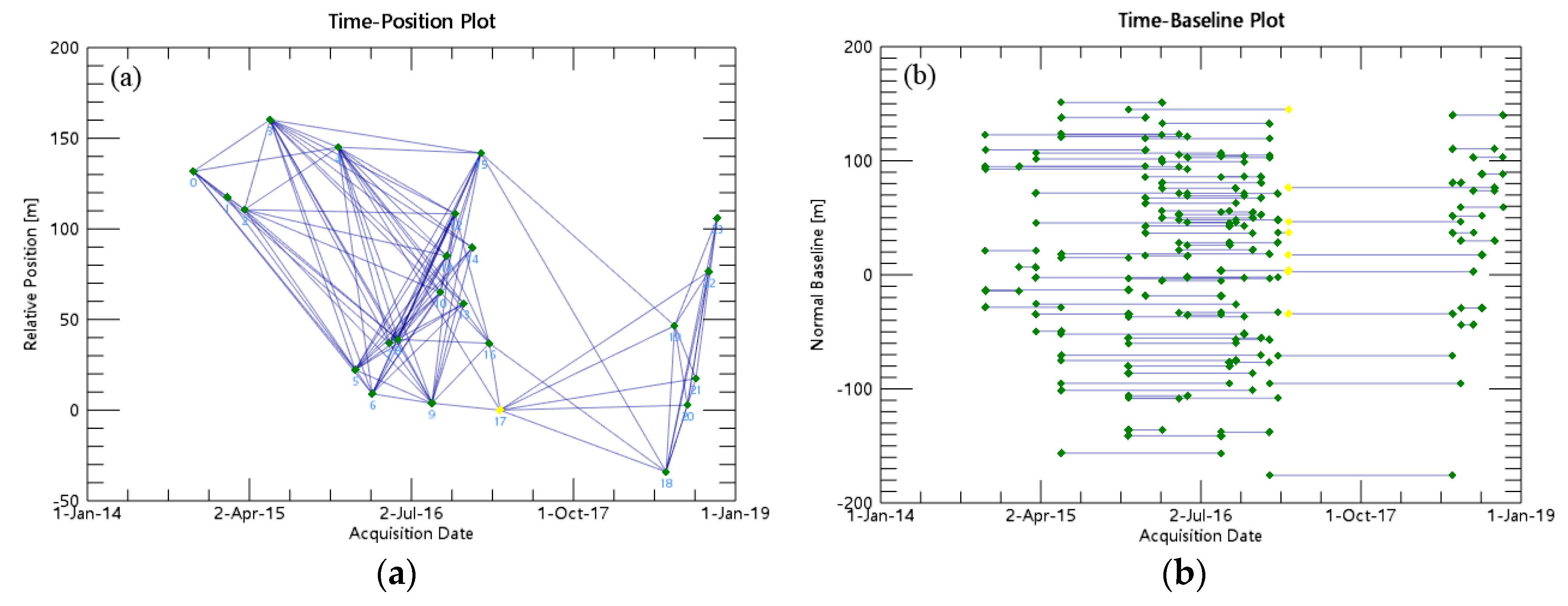
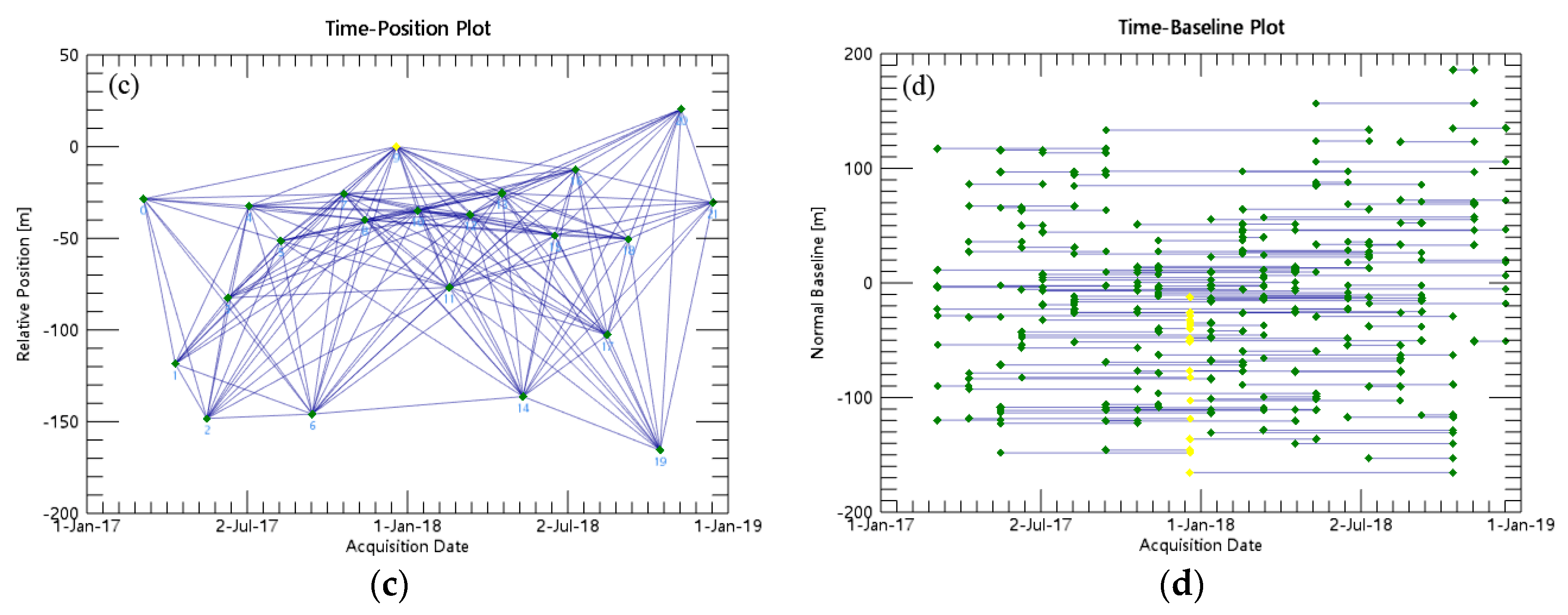
The first step was to graphically output the generated interferograms. When the SAR images are entered alongside the spatial and temporal baseline threshold, the maximum logarithm that can be obtained was (N × (N−1))/2, and the tool would automatically select the best combination for pairing. In this study, a 50% spatial baseline of the critical baseline and time baseline was set to 365 days. These pairs were interfering and then used for SBAS inversion (Figure 2). The program automatically selected a super master image, which was used as the reference image throughout the process, and all the pairs were registered to the super master image [17].

The second step was to interfere with all the paired interference image pairs, including coherence generation, de-leveling, filtering, and phase unwrapping. All the data pairs were registered to the super-master image. What is important in this step was to obtain a satisfactory interferogram by adjusting the parameters and coefficients. Thus, the interferogram showed part of the low coherence area, and after the first screening, we chose to increase the intensity of the filter strength. The Goldstein filtering method is a commonly filtering method. In this study, the processing tools of the interference processing module were used to process some representative image pairs to debug the satisfactory processing parameters. After the second screening, the phase unwrapped graph was checked to determine if the coherence threshold needs to be adjusted until a satisfactory result was obtained. Finally, the unwrapping method this paper used was Delaunay Minimum Cost Flow (MCF), which was a good way to connect a set of high-coherence pixels and other isolated high-coherence regions, thus this method was recommended to minimize the impact of phase transitions.

The third step was to remove the constant phase and phase transitions that still exist in the unwrapped phase diagram, resulting in a re-leveling result. In SARscape, there were two optimization methods on the flattening parameter panel: orbit optimization and residual phase optimization. This paper used an orbital optimization method that utilized an orbital polynomial model to correct the orbital parameters of the secondary image to eliminate the ramp phase.

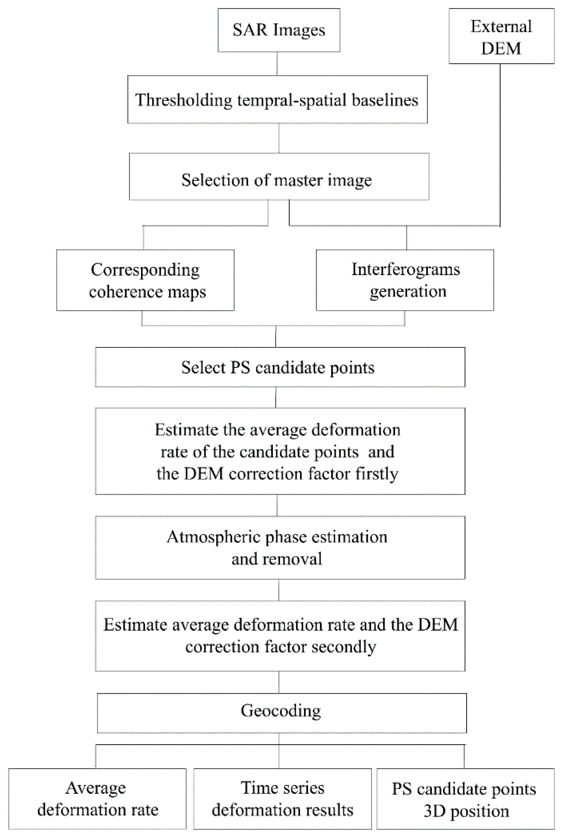
The next step was to estimate the deformation rate and residual topography, and reduce the atmospheric phase as much as possible by filtering. Atmospheric filtering played a role in the smoothing of the time series. The removal of the atmosphere was achieved by low-pass filtering and high-pass filtering. Finally, the deformation results in the time series were obtained. The software not only calculated the deformation rate of the Line-Of-Sight (LOS) direction, but also the vertical direction. This study used the deformation results in the vertical direction for analysis [17]. Finally, the deformation results in the time series were obtained. The software not only calculated the deformation rate of the LOS direction, but also the vertical direction. This study used the deformation results in the vertical direction for analysis. The technical flow chart is shown in Figure 3.

3.2. Acquisition of Building Area

The building area during the same period was acquired using the classification results of Landsat 8. The detailed information of workflow was divided into three parts. Firstly, the Landsat 8 OLI image that was achieved was pre-processed. Secondly, the land cover information was extracted by the object coverage classification method, which was verified with the traditional supervised classification and ground observations. Finally, the southern architectural coverage map along the Erhai region was obtained.

The original image was radiated and calibrated with the radiation calibration parameters of the OLI sensor, and the Digital Number (DN) value of the original image was transformed into the radiance by pixel scale. Then, the image was corrected using the Fast Line-of-sight Atmospheric Analysis of Hypercubes (FLAASH) model, and the radiance value was converted into the true reflectance of the surface [46,47]. In addition, geometric precision correction was performed on the image, making the correction error controlled within 0.1 pixel. Finally, the Gram–Schmidt algorithm was used to fuse band 2, band 3, and band 4 of the corrected image, and the resolution of the fused image was 30 meters, which was helpful to the extraction of urban building classification information. Supervised classification was based on prior knowledge and trained by selecting samples in order to establish statistical recognition function and classify categories according to probability rules. The application of this method of classifying land use could guarantee the reliability and representativeness of the results. In this study, ENVI 5.3 software was used as the operating platform, and the maximum likelihood algorithm was used to supervise and classify remote sensing images in the Erhai region. This research distinguished elements visually on the image and drew the polygon samples, and tried to ensure the purity of the elements in the sample. It also drew other samples of the feature in other areas, and the sample was distributed as evenly as possible across the image. According to the research needs, the selected land-use samples were building land, water, agriculture, forest land, and bare land. The training samples were selected according to the characteristics of the land-covering classification scheme and the sample description. The sample selection followed the principle of uniform distribution of the entire study area, and the region of interest was established through the visual interpretation in the Landsat 8 OLI image, combined with Google Earth high image optimization. In order to check the separability between each sample, the Jeffries–Matusita, Transformed Divergence parameters were used to investigate. When the values of those two parameters were between 0 and 2.0, greater than 1.9 indicated that the sample was separable and belonged to the qualified sample; less than 1.8 indicate a need to edit the sample or re-select the sample; less than 1 considered combining the two types of samples into a sample. The sample classification results were tested, and separation values of different types were greater than 1.9, which meant that the samples taken can be well differentiated. According to the classification of representative training samples, the maximum likelihood classification method was adopted in the southern Erhai region to obtain the building area. The classification accuracy was evaluated, and the classification results were compared with the sample points obtained in the field survey to verify the accuracy of the results. The data format of the urban building area extraction result was converted into the shape format, and the urban building area data was extracted in ArcGIS 10.4 to obtain the specific data of the building area of the Erhai region that belong to different times.

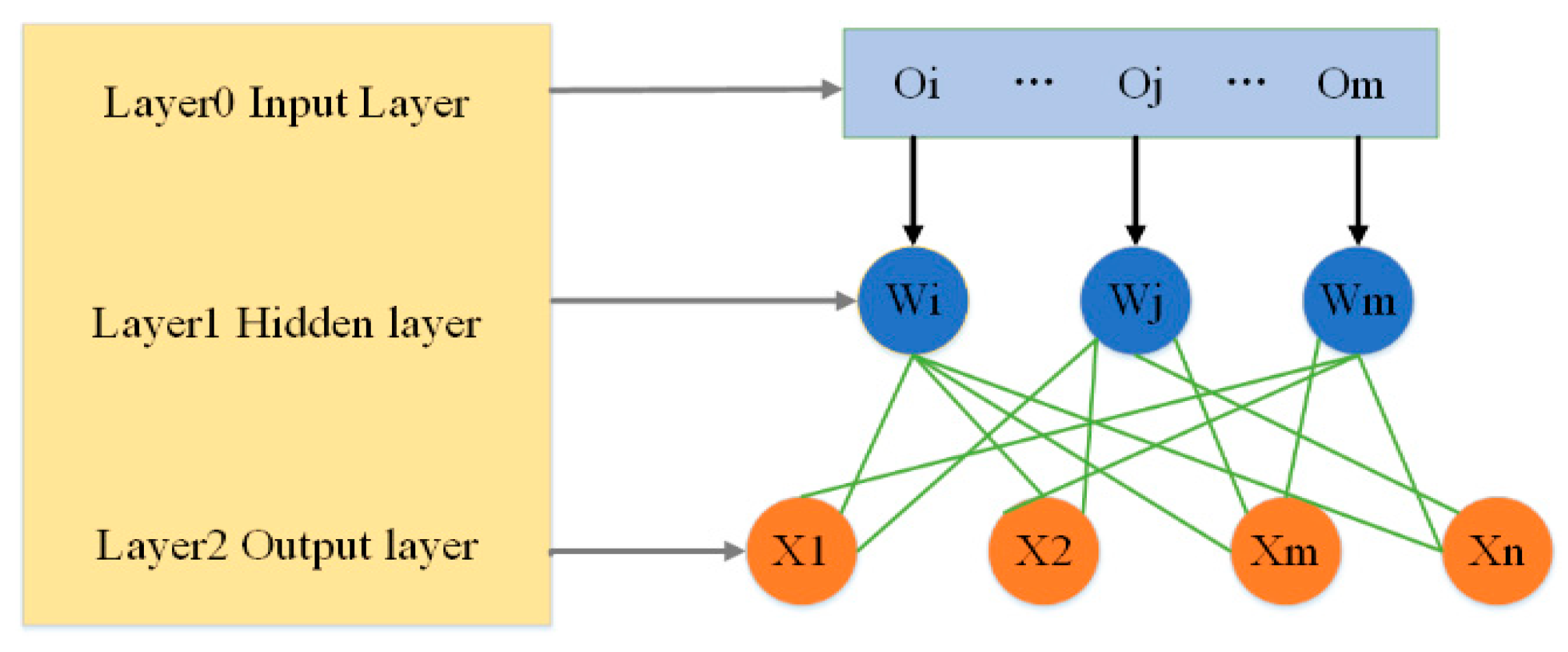
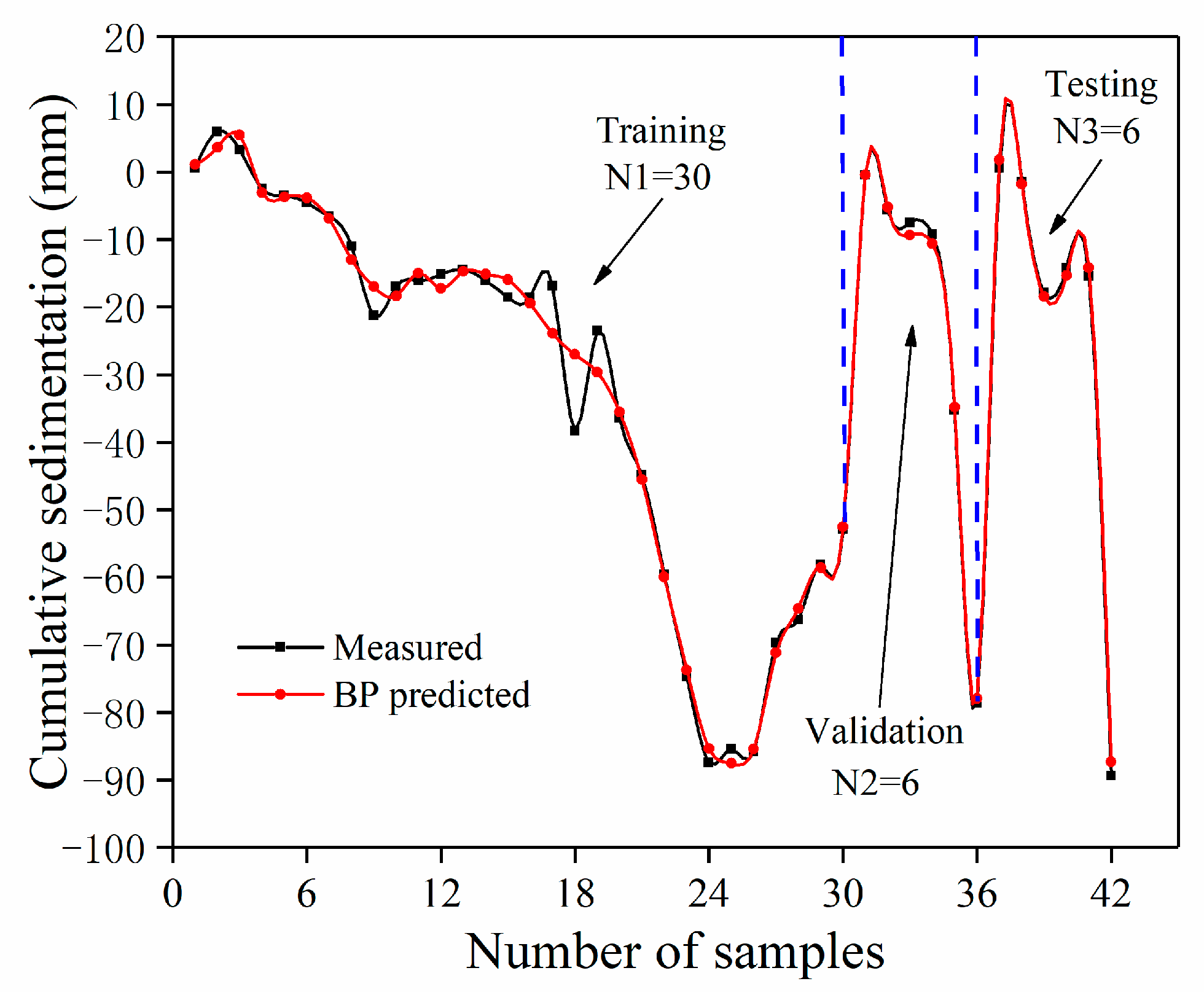
3.3. Predicting the Cumulative Ground Deformation Using Back-Propagation

Predicting the cumulative ground deformation was required in many fields associated with urbanization, environment protection, agricultural, and ecological applications [48,49]. However, the current prediction methods were either using linear regression or multiple linear regression. In other words, the current analysis or predicting of cumulative ground deformation was mainly dependent on the previous results of ground deformation [50,51]. The predicting was based on the analysis of the current condition; therefore, the relationships built from linear or multiple linear regression were so simple that their uncertainties of predicted results cannot be easily controlled. Then, the predicting results were not convincing or reliable. To face this challenge, a more reliable model with precise data should be built and adopted. BP is a supervised learning method of Artificial Neural Networks (ANN), which can be used to perform a given task [52,53,54]. It requires a teacher who knows, or can calculate, the desired output for any input in the training set. 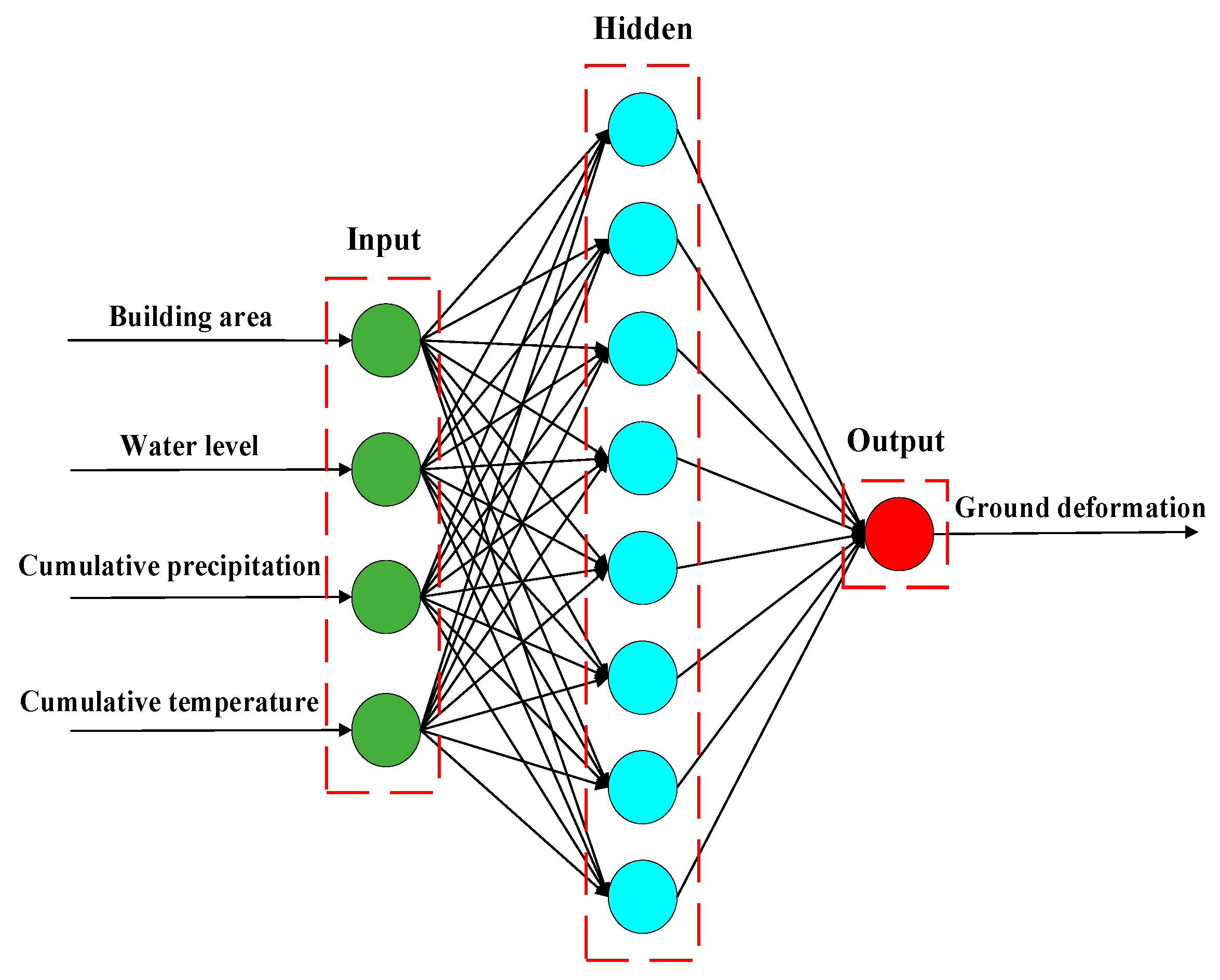BP requires that the activation function used by the artificial neurons (or “nodes”) be differentiable [55,56,57]. Therefore, the ANN was adopted to predict the cumulative ground deformation using related independent variables such as temperature, precipitation, water level, or building area. For a given region, the related influencing factors are used as model input parameters, and the cumulative ground deformation is set as a model output parameter. The whole process needs to consider the input, output, network, node, study rate, et al.

$$\mathrm{l}=\sqrt{m+n}+\epsilon , \epsilon =0, 1, 2,\dots , 10$$

(5)

In the equation, $l$ represents the number of hidden nodes; $m$ represents the number of input nodes; $n$ represents the number of output nodes, and $\epsilon$ represents the constant.

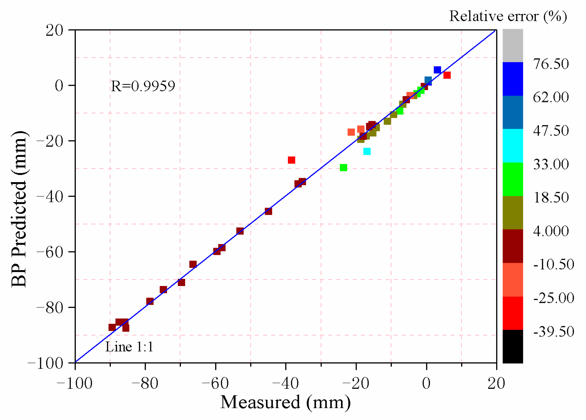
Indicators such as the root mean square error (RMSE) are selected to evaluate the precision of the simulated versus the observed data. The RMSE reflects the distance of the training sample, testing sample, and validating sample from the real data or true data. The RMSE is defined as follows [58]:

$$\mathrm{RMSE}=\left(\frac{{{\displaystyle \sum }}_{i=1}^n{\left(S_i-O_i\right)}^2}{n}\right)$$

(6)

In the equations, $S_i$ represents the simulated results; $O_i$ represents the observed results; $\overline{O_i}$ is the mean value of the observed data, and n is the total number of comparisons. The basic process of BP was shown in Figure 4, and the detailed workflow is defined as follows:

Normalization

For most machine learning and optimization algorithms, scaling the eigenvalues to the same interval makes it possible to obtain better performance models. For example, there are two different features. The first feature ranges from 1 to 10, and the second feature ranges from 1 to 10,000. In the gradient descent algorithm, the cost function was the least square error function. Therefore, when it comes to the algorithm, the second feature will be obviously chosen when using the gradient descent algorithm, because it has a larger range of values.

Propagation

The forward propagation of a training pattern’s input through the neural network was to generate the propagation’s output activations. Then, the BP of the propagation’s output activations through the neural network using the training pattern’s target was to generate the deltas of all the output and hidden neurons.

Weight Update

First, we multiply the output delta and input activation to get the gradient of the weight. Then, we bring the weight in the opposite direction of the gradient by subtracting a ration of it from the weight.

4. Results

4.1. Deformation Results

4.1.1. Mean Deformation Rate Map

Figure 5 shows the average annual ground deformation from 2015 to 2018 in the Erhai region by using SBAS-InSAR. The figure was superimposed by the reflection of the intensity information of the SAR image, where the positive values of the rate map indicate that the surface was uplifting in the vertical direction, and the negative values denote surface deformation in the same direction. The SBAS-InSAR-derived results are shown in Figure 4; the annual average deformation rates in the Erhai region ranged from −33 to 9 mm/year. In the northern part of the Erhai region, the surface did not show obvious deformation; however, ground deformation was mainly concentrated in the southern Erhai region, with the most serious observation points reaching an average of −33 mm/year.

4.1.2. Time Series of Deformation

Figure 6 shows the surface interannual cumulative deformation time series in the Erhai region from 2015 to 2018. The magnitude of deformation in the southern part of the deformation areas gradually increased from 2015 to 2017, and the size of these deformation areas also gradually expanded; however, changes in the ground magnitude and range were small between 2017 and 2018, and some places even showed a rebound. In contrast, the northern Erhai region did not show ground deformation.

4.1.3. The Validation of Results

To quantitatively verify the accuracy of the surface deformation monitoring using Sentinel-1 SAR images and SBAS-InSAR, a cross-validation of differences between descending and ascending SAR image-derived results were performed. This study used the deformation results in the vertical direction for analysis because the ground deformation of the descending and ascending images was inconsistent with the line of sight. The two sets of SAR images had overlapped part of the time series, from June 2018 to November 2018 (six months); thus the differences during the overlapped timing sequence were used to test these two result sets. Figure 7 shows the differences between the two sets of results calculated using the ArcGIS 10.4 raster calculator function.

Using SAR images, the data statistics of different deformation results (descending and ascending) were calculated. In order to cross-validate the results, the difference between the two data sets was taken. The results of the difference statistics are shown in

Table 3. Data Analysis Results.

Interval Center Value	Counts	Data Summation	Cumulative Percentage
−85	2	2	0.0006%
−75	4	6	0.002%
−65	43	49	0.015%
−55	9	58	0.018%
−45	139	197	0.062%
−35	1120	1317	0.413%
−25	7687	9004	2.822%
−15	53739	62743	19.667%
−5	136255	198998	62.375%
5	89627	288625	90.468%
15	29891	318516	99.837%
25	417	318933	99.968%
35	61	318994	99.987%
45	12	319006	99.991%
55	14	319020	99.995%
65	6	319026	99.997%
75	5	319031	99.999%
85	5	319036	100%

, with different intervals for data statistics, including the number of distributions and the cumulative percentage. As shown in Figure 8, the distribution statistics of the verification results and the fitted normal curves were obtained. When the difference was 0, it was proven that the two sets of data are completely consistent. The results of the verification were mainly distributed in the range of −5 mm to 5 mm, wherein the data in the range of −5 mm to 0 mm accounted for 42.70%, and the data range from 0 mm to 5 mm accounted for 28.10%. The average difference, maximum (MAX), and minimum (MIN) totaled −2.5, 81.23, and −83.04 mm, respectively. According to Figure 7, the deviation of the Erhai region from the mountain was slightly larger, with an absolute value between 20−40 mm. Due to the slope instability and the coverage of surface vegetation, the SBAS-InSAR method was prone to errors in the vicinity of the mountains. However, most of the validation results in the study area were less than 10 mm, including the distribution of southern urban agglomerations and most rural areas, indicating that the two sets of data were well tested, and the ground deformation rate calculations were reliable.

4.2. Correlation between Ground Deformation and Factors

4.2.1. Urbanization Rate of Dali City

Urbanization has been a key issue among scholars concerning the development and modernization of China and other developing countries. [59,60,61] used a parameter of urbanization to quantify the results, which was generally defined as the proportion of the urban population in the total population (including the agricultural and non-agricultural population) [62]. From the statistical yearbook, the relevant data from 2014 to 2017 of Dali City and the relevant calculation results are shown in

Table 4. Urbanization Data of Dali City.

Year	Total Population	Urban Population	Rural Population	Building Area/ha	Urbanization Rate
2017	3,584,000	1,637,171	1,946,828	83,600	45.68%
2016	3,563,000	1,569,000	1,994,000	82,500	44.04%
2015	3,544,000	1,495,922	2,048,077	80,910	42.21%
2014	3,527,000	1,429,000	2,098,000	78,693	40.52%

. The total population and urban population of Dali City were increasing; thus, the proportion of the rural population was decreasing gradually, which led to the increasing trend of the urbanization rate from 2014 to 2017, where the city’s urbanization rate increased by 5%. In addition, the construction area of Dali City was also expanding, which reflected the current situation of local urban expansion in the local region.

According to the research needs, the selected land-use samples were building land, water region, agriculture, forest land, and bare land. After the completion of different types of land-use selection samples, the sample accuracy was checked, and the mixed matrix of classification templates was calculated in order to ensure that dispersion between different types of samples was maintained at more than 1.9. The separation of analysis types was checked in n-dimensional visualization, and sample points were modified. The difference result distribution was shown in Figure 9.

Through the vector results, the building area in the south of the Erhai region was calculated. As shown in

Table 5. Statistics of Building Area in the Southern Region of Erhai.

Date (y/m/d)	2015/02/03	2016/01/05	2016/12/06	2017/12/25	2018/11/26
covered area (ha)	8183.19	8247.31	8308.53	8375.84	8407.98

, the building area of the region showed a steady increasing trend. From February 2015 to December 2017, the building area increased by 4.28 ha annually. However, from December 2017 to November 2018, the building area increased by 2.14 ha, which indicated that the rate of urban expansion had slowed down. It could explain that the ground deformation rate in the southern Erhai region decreased from 2017 to 2018.

4.2.2. Analysis of Influencing Factors to Ground Deformation

The surrounding environmental factors have certain impacts on the ground deformation [63,64,65,66,67]. Reasons for the happening of ground deformation in the southern Erhai region were analyzed, and the prediction of the future deformation was carried out accordingly. The cumulative monthly deformation data of the severe deformation area in the southern Erhai region were calculated, and the correlations between the cumulative temperature, cumulative precipitation, urban building area, and water level were tested to obtain the fitting equation, and their linear correlation coefficients (R²) were shown in Figure 10. The R² between cumulative deformation and four factors were 0.764, 0.746, 0.431, and 0.113, respectively.

4.3. Results of Predicting the Cumulative Ground Deformation Using BP

As indicated in the methodology, the data were normalized to the scale from 0 to 1 to improve the prediction precision. Then, the independent variables of temperature, precipitation, water level, and building area were used to calculate relationships with the dependent variable cumulative ground deformation using BP. The independent variables were set as input parameters, and the cumulative ground deformation was set as the output parameter. The number of hidden nodes was calculated using Equation (5), and the optimal set of the number of hidden nodes was confirmed through a variety of experiments. The final set of numbers of hidden notes was eight. The study rate will influence both the study speed and study precision; when the study rate is small, the time will be longer, and the precision will be higher; while in contrast, when the study rate is large, the time will be shorter, and the precision will be less. Besides, as the times of training increased, the errors of samples were actually not decreasing, or even growing bigger. Therefore, there is no necessity to training anymore with this condition, because overtraining will probably lead to overfitting. In order to solve this problem, the training will continue constantly until one of the following conditions was satisfied: (1) the iteration is 100 times; (2) the mean square error of the target of the sample training is below 0.001; (3) in the process of the network using training samples, the error curve of the validated sample will not decline for six consecutive iterations. In this study, the error curve of the validated sample did not decrease after more than six iterations. Therefore, the training network was stopped, and the time of iteration was 67. According to Figure 11, a 4-8-1 BP model was built: the model was confirmed with four input parameters, eight hidden nodes, and one output parameter.

The independent variables of temperature, precipitation, water level, and building area were set as input parameters, and the cumulative ground deformation was set as the output parameter. In this study, 42 sets of sample data were used to construct the model, of which 30 sets of randomly extracted data were training samples, another six sets of data were randomly extracted as validation samples, and the last six sets of data were used as test samples. Figure 12 clearly showed the fitting results were good with 42 sets of total samples, 30 sets groups of training samples, six sets of validating samples, and six other testing samples. The training sample, the comparison between the verification sample, and the test sample indicated that the constructed BP neural network model had obtained a good predictive effect.

In order to quantify and assess the performance of the BP network, the R and root mean square error (RMSE) were each calculated. Figure 13 and

Table 6. Root Mean Square Error (RMSE) between Training Sample, Testing Sample, Validating Sample, and Real Data.

Sample	Training	Testing	Validating
RMSE/mm	3.063	1.003	1.119

show the correlations between predicted results and the real data. The most relative error appearance was between −10.5% and 33%, and the R was confirmed as 0.996. When the iteration was added, the RMSE will grow low; this process was repeated hundreds of times to reduce the random error in the data and obtain stable and reliable results. When the RMSE was stabilized, the results showed that the RMSE displayed using the validating samples showed that the results had a relatively low error. The RMSE of the training sample, the test sample, the verification sample, and the actual data were 3.063, 1.003, and 1.119, respectively. Through the RMSE of the testing sample, it can be deduced that the error between the predicted cumulative ground deformation and the real data can be reduced to 1 mm using the BP network. In conclusion, the high R and small RMSE showed that the built model BP network model had obtained relatively high precision. The model performed quite well for predicting the potential cumulative ground deformation.

5. Discussion

5.1. Deformation Results

As shown in Figure 6 and Figure 7, the results in the northern Erhai region were stable and a distorted phenomenon was not obvious. However, the deformation in the southern Erhai region was particularly obvious, especially in the southeastern part. According to Figure 9, referring to the results of R² analysis, it was found that the temperature, precipitation, and water level of the lake and building area have a certain influence on the ground deformation. The seasonality of regional ground deformation was reflected in the changes to the temperature and precipitation data. Accordingly, the R² results of the two data sets and ground deformation were above 0.7, indicating that the ground deformation along the southern region of Erhai had a certain seasonal regularity. In addition, the urban agglomerations along the Erhai region were mainly distributed in the southeastern part. The R² results indicated that there was a strong correlation between the building area and the ground deformation results. Moreover, there was also a certain relationship between the water level and ground deformation, but the evaluation results were lower than those of the former.

In the Erhai region, meteorological elements and water-level data were consistent across the research area; however, the ground deformation results of the southern and northern regions were completely different, which indicated the important influence of the building expansion during the process of ground deformation. The northern part of Erhai was mainly cultivated by crops, and the urban distribution was relatively scattered. There were no large areas of urban agglomeration. However, the building area in the southern area was densely populated, with few individual farmland distributions, showing an increasing distorted trend over the years. Therefore, a comparison of the two regions in the north and the south shows that the development and expansion of the city were the main reasons for the ground deformation in the southern Erhai region. The water-level height can affect the coastal groundwater and have a certain effect on the ground deformation [68]. The urban distribution and seasonal changes of the water level were the impact factors that caused the fluctuation of ground deformation.

5.2. Future Deformation Prediction

In this study, the machine learning BP was used to predict the ground deformation; the results shown in Section 4 indicated that machine learning has great potential for predicting the ground deformation. There are many kinds of machine learning methods such as BP, Random Forest, and Support Vector Machine (SVM). BP was adopted because this method was commonly used and can be easily deployed. Besides, the BP was more precise than the linear regression and multiple linear regression. Since the machine learning has shown great ability to predict the ground deformation, the adoption of advanced methods would be introduced. Through using a long time series of high-resolution independent data and the Deep Learning (DL) method, the ground deformation can be precisely predicted. Both the analysis of SAR images and machine learning prediction of obtaining the ground deformation would stress some greater useful information than the adoption of a single method. This would likely provide useful information to city planning, especially the building of important sites such as airports and highways. The prediction results make it possible to guide the designing to avoid serious ground deformation, which could happen in some places in the future. In order to obtain a more reliable prediction result, Deep Learning (DL) could be adopted, which had a greater depth of nodes, and thus would likely reduce the random uncertainties and systemic errors.

5.3. Countermeasures and Suggestions

The southeastern part of the Erhai region was the main area where deformation exists. Monitoring and early warning should be strengthened in this place by constructing a regional ground deformation management network and building a monitoring network. Only by the timely understanding of the regional ground deformation can people take appropriate measures to avoid the catastrophic consequences. People should rationally construct the northern shore of the Erhai region in order to balance the development between the north and the south. This method could alleviate the urbanization problem of the southern region, in order to solve the condition of the ground deformation in that area. Since the development of the city was the main cause of ground deformation in the Erhai region, people must grasp a certain scale for urbanization without over-exploring in a short period time. The load effect during building exploring will have a series of effects on the ground, which will lead to ground deformation. Other studies have shown that excessive groundwater exploitation may also cause ground deformation [69,70]. Although the Erhai area is close to lakes and rich in water resources, the local government still should establish awareness of water protection, such as from water pollution and so on.

Erhai Lake is the second largest lake in Yunnan Province and ranks seventh among China’s freshwater lakes. It has important ecological functions and tourism value. Focusing on standardizing the environmental management, improving environmental quality, and promoting the sustainable development of tourism are needed in the Erhai region.

6. Conclusions

In this study, the ground deformation results of the Erhai region from 2015 to 2018 were obtained by performing SBAS-InSAR technology on a total of 44 ascending and descending Sentinel-1 images. Based on the four variables of temperature, precipitation, and water level of the lake and building area, the causal factors for the ground deformation were analyzed, which indicated that urban construction is the main cause of ground deformation disaster in the region of Erhai. The back-propagation (BP) algorithm was used to predict and verify the ground deformation of the study area with high precision, and some reasonable suggestions were made accordingly. The point of this research was that the introduction of the back-propagation algorithm into the prediction of regional ground deformation was used for the first time, which could provide a reference for future correlation research.

References

1. Bekaert, D.P.; Jones, C.E.; An, K.; Huang, M.-H. Exploiting UAVSAR for a comprehensive analysis of subsidence in the Sacramento Delta. Remote Sens. Environ. 2019, 220, 124–134. [Google Scholar] [CrossRef]
2. Gao, M.; Gong, H.; Chen, B.; Zhou, C.; Chen, W.; Liang, Y.; Shi, M.; Si, Y. InSAR time-series investigation of long-term ground displacement at Beijing Capital International Airport, China. Tectonophysics 2016, 691, 271–281. [Google Scholar] [CrossRef]
3. Bell, F.G.; Stacey, T.R.; Genske, D.D. Mining subsidence and its effect on the environment: Some differing examples. Environ. Earth Sci. 2000, 40, 135–152. [Google Scholar] [CrossRef]
4. Alloy, A.; Gonzalez Dominguez, F.; Nila Fonseca, A.L.; Ruangsirikulchai, A.; Gentle, J.N., Jr.; Cabral, E.; Pierce, S.A. Development of an expert analysis tool based on an interactive subsidence hazard map for urban land use in the city of Celaya, Mexico. In AGU Fall Meeting Abstracts; American Geophysical Union: Washington, DC, USA, 2016. [Google Scholar]
5. Stramondo, S.; Bozzano, F.; Marra, F.; Wegmuller, U.; Cinti, F.; Moro, M.; Saroli, M. Subsidence induced by urbanisation in the city of Rome detected by advanced InSAR technique and geotechnical investigations. Remote Sens. Environ. 2008, 112, 3160–3172. [Google Scholar] [CrossRef]
6. Castellazzi, P.; Arroyo-Domínguez, N.; Martel, R.; Calderhead, A.I.; Normand, J.C.; Gárfias, J.; Rivera, A. Land subsidence in major cities of Central Mexico: Interpreting InSAR-derived land subsidence mapping with hydrogeological data. Int. J. Appl. Earth Obs. Geoinf. 2016, 47, 102–111. [Google Scholar] [CrossRef]
7. Huanhuan, L.; Youquan, Z.; Rong, W. The reason of land subsidence and prevention measures of Beijing segment of Beijing-Tianjin high-speed rail. In Proceedings of the 2014 Third International Workshop on Earth Observation and Remote Sensing Applications (EORSA), Changsha, China, 11–14 June 2014; pp. 323–325. [Google Scholar]
8. Yang, C.-S.; Zhang, Q.; Zhao, C.-Y.; Wang, Q.-L.; Ji, L.-Y. Monitoring land subsidence and fault deformation using the small baseline subset InSAR technique: A case study in the Datong Basin, China. J. Geodyn. 2014, 75, 34–40. [Google Scholar] [CrossRef]
9. Ng, A.H.-M.; Ge, L.; Li, X.; Zhang, K. Monitoring ground deformation in Beijing, China with persistent scatterer SAR interferometry. J. Geodyn. 2012, 86, 375–392. [Google Scholar] [CrossRef]
10. Kim, J.-W.; Lu, Z.; Jia, Y.; Shum, C. Ground subsidence in Tucson, Arizona, monitored by time-series analysis using multi-sensor InSAR datasets from 1993 to 2011. ISPRS J. Photogramm. Sens. 2015, 107, 126–141. [Google Scholar] [CrossRef]
11. Sharma, P.; Jones, C.E.; Dudas, J.; Bawden, G.W.; Deverel, S. Monitoring of subsidence with UAVSAR on Sherman Island in California’s Sacramento–San Joaquin Delta. Remote Sens. Environ. 2016, 181, 218–236. [Google Scholar] [CrossRef]
12. Ying, M.; Zhang, W.; Yu, H.; Lu, X.; Feng, J.; Fan, Y.; Zhu, Y.; Chen, D. An Overview of the China Meteorological Administration Tropical Cyclone Database. J. Atmos. Ocean. Technol. 2014, 31, 287–301. [Google Scholar] [CrossRef]
13. Massonnet, D.; Feigl, K.L. Radar interferometry and its application to changes in the Earth’s surface. Rev. Geophys. 1998, 36, 441–500. [Google Scholar] [CrossRef]
14. Colesanti, C.; Ferretti, A.; Novali, F.; Prati, C.; Rocca, F. Sar monitoring of progressive and seasonal ground deformation using the permanent scatterers technique. IEEE Trans. Geosci. Sens. 2003, 41, 1685–1701. [Google Scholar] [CrossRef]
15. Cascini, L.; Peduto, D.; Réale, D.; Arena, L.; Ferlisi, S.; Verde, S.; Fornaro, G. Detection and monitoring of facilities exposed to subsidence phenomena via past and current generation SAR sensors. J. Geophys. Eng. 2013, 10, 64001. [Google Scholar] [CrossRef]
16. Amighpey, M.; Arabi, S. Studying land subsidence in Yazd province, Iran, by integration of InSAR and levelling measurements. Sens. Appl. Soc. 2016, 4, 1–8. [Google Scholar] [CrossRef]
17. Rosen, P.A.; Hensley, S.; Joughin, I.R.; Li, F.K.; Madsen, S.N.; Rodriguez, E.; Goldstein, R.M. Synthetic aperture radar interferometry. Proc. IEEE 2002, 88, 333–382. [Google Scholar] [CrossRef]
18. Atzori, S.; Hunstad, I.; Chini, M.; Salvi, S.; Tolomei, C.; Bignami, C.; Stramondo, S.; Trasatti, E.; Antonioli, A.; Boschi, E. Finite fault inversion of DInSAR coseismic displacement of the 2009 L’Aquila earthquake (central Italy). Geophys. Lett. 2009, 36. [Google Scholar] [CrossRef]
19. Ge, L.; Chang, H.-C.; Rizos, C. Mine Subsidence Monitoring Using Multi-source Satellite SAR Images. Photogramm. Eng. Sens. 2007, 73, 259–266. [Google Scholar] [CrossRef]
20. Trasatti, E.; Casu, F.; Giunchi, C.; Pepe, S.; Solaro, G.; Tagliaventi, S.; Berardino, P.; Manzo, M.; Pepe, A.; Ricciardi, G.P.; et al. The 2004-2006 uplift episode at Campi Flegrei caldera (Italy): Constraints from SBAS-DInSAR ENVISAT data and Bayesian source inference. Geophys. Lett. 2008, 35. [Google Scholar] [CrossRef]
21. Ding, R.; Xu, J.; Lin, X.; Xu, K. Monitoring of surface subsidence using PSInSAR with TerraSAR-X high resolution data. Remote Sens. Land Resour. 2015, 27, 158–164. [Google Scholar]
22. Canova, F.; Tolomei, C.; Salvi, S.; Toscani, G.; Seno, S. Land subsidence along the Ionian coast of SE Sicily (Italy), detection and analysis via Small Baseline Subset (SBAS) multitemporal differential SAR interferometry. Earth Surf. Process. Landf. 2012, 37, 273–286. [Google Scholar] [CrossRef]
23. Lanari, R.; Casu, F.; Manzo, M.; Lundgren, P. Application of the SBAS-DInSAR technique to fault creep: A case study of the Hayward fault, California. Remote Sens. Environ. 2007, 109, 20–28. [Google Scholar] [CrossRef]
24. Tizzani, P.; Berardino, P.; Casu, F.; Euillades, P.; Manzo, M.; Ricciardi, G.; Zeni, G.; Lanari, R. Surface deformation of Long Valley caldera and Mono Basin, California, investigated with the SBAS-InSAR approach. Remote Sens. Environ. 2007, 108, 277–289. [Google Scholar] [CrossRef]
25. Zhao, R.; Li, Z.-W.; Feng, G.-C.; Wang, Q.-J.; Hu, J. Monitoring surface deformation over permafrost with an improved SBAS-InSAR algorithm: With emphasis on climatic factors modeling. Remote Sens. Environ. 2016, 184, 276–287. [Google Scholar] [CrossRef]
26. Gee, D.; Sowter, A.; Novellino, A.; Marsh, S.; Gluyas, J. Monitoring land motion due to natural gas extraction: Validation of the Intermittent SBAS (ISBAS) DInSAR algorithm over gas fields of North Holland, the Netherlands. Mar. Pet. Geol. 2016, 77, 1338–1354. [Google Scholar] [CrossRef]
27. Manunta, M.; Marsella, M.; Zeni, G.; Sciotti, M.; Atzori, S.; Lanari, R. Two-scale surface deformation analysis using the SBAS-DInSAR technique: A case study of the city of Rome, Italy. Int. J. Sens. 2008, 29, 1665–1684. [Google Scholar] [CrossRef]
28. Zeni, G.; Bonano, M.; Casu, F.; Manunta, M.; Manzo, M.; Marsella, M.; Pepe, A.; Lanari, R. Long-term deformation analysis of historical buildings through the advanced SBAS-DInSAR technique: The case study of the city of Rome, Italy. J. Geophys. Eng. 2011, 8, S1–S12. [Google Scholar] [CrossRef]
29. Dong, S.; Samsonov, S.; Yin, H.; Ye, S.; Cao, Y.J. Time-series analysis of subsidence associated with rapid urbanization in Shanghai, China measured with SBAS InSAR method. Environ. Earth Sci. 2014, 72, 677–691. [Google Scholar] [CrossRef]
30. Xu, B.; Feng, G.; Li, Z.-W.; Wang, Q.; Wang, C.; Xie, R. Coastal Subsidence Monitoring Associated with Land Reclamation Using the Point Target Based SBAS-InSAR Method: A Case Study of Shenzhen, China. Remote Sens. 2016, 8, 652. [Google Scholar] [CrossRef]
31. Zhou, L.; Guo, J.; Hu, J.; Li, J.; Xu, Y.; Pan, Y.; Shi, M. Wuhan Surface Subsidence Analysis in 2015–2016 Based on Sentinel-1A Data by SBAS-InSAR. Remote Sens. 2017, 9, 982. [Google Scholar] [CrossRef]
32. Wang, X.; Zhang, Y.; Jiang, X.; Zhang, Z. A dynamic prediction method of deep mining subsidence combines d-insar technique. Procedia Environ. Sci. 2011, 10, 2533–2539. [Google Scholar]
33. Murphy, K.P. Machine Learning: A Probabilistic Perspective; MIT Press: Cambridge, MA, USA, 2012. [Google Scholar]
34. Blum, A.L.; Langley, P. Selection of relevant features and examples in machine learning. Artif. Intell. 1997, 97, 245–271. [Google Scholar] [CrossRef]
35. Rouet-Leduc, B.; Hulbert, C.; Lubbers, N.; Barros, K.; Humphreys, C.J.; Johnson, P.A.; Rouet-Leduc, B. Machine Learning Predicts Laboratory Earthquakes. Geophys. Lett. 2017, 44, 9276–9282. [Google Scholar] [CrossRef]
36. Li, B.; Tang, C.; Zheng, T.; Lei, Z. Fully automated extraction of the fringe skeletons in dynamic electronic speckle pattern interferometry using a U-Net convolutional neural network. Opt. Eng. 2019, 58, 023105. [Google Scholar] [CrossRef]
37. Anantrasirichai, N.; Biggs, J.; Albino, F.; Hill, P.; Bull, D. Application of Machine Learning to Classification of Volcanic Deformation in Routinely Generated InSAR Data. J. Geophys. Res. Solid Earth 2018, 123, 6592–6606. [Google Scholar] [CrossRef]
38. Wang, Y.; Pang, H.; Wu, Q.; Huang, Q. Impacts of human activity on Erhai Lake and countermeasures. J. Lakeence 1999, 11, 123–128. [Google Scholar]
39. Minderhoud, P.; Coumou, L.; Erban, L.; Middelkoop, H.; Stouthamer, E.; Addink, E. The relation between land use and subsidence in the Vietnamese Mekong delta. Sci. Total. Environ. 2018, 634, 715–726. [Google Scholar] [CrossRef] [PubMed]
40. Sowter, A.; Amat, M.B.C.; Cigna, F.; Marsh, S.; Athab, A.; Alshammari, L. Mexico City land subsidence in 2014–2015 with Sentinel-1 IW TOPS: Results using the Intermittent SBAS (ISBAS) technique. Int. J. Appl. Earth Obs. Geoinf. 2016, 52, 230–242. [Google Scholar] [CrossRef]
41. Gorokhovich, Y.; Voustianiouk, A. Accuracy assessment of the processed SRTM-based elevation data by CGIAR using field data from USA and Thailand and its relation to the terrain characteristics. Remote Sens. Environ. 2006, 104, 409–415. [Google Scholar] [CrossRef]
42. National Meteorological Information Center. 2017. Available online: http://data.cma.cn/ (accessed on 15 May 2019).
43. Liu, Z.; Li, L.; Tim, R.M.; Vanniel, T.G.; Yang, G.; Li, R. Introduction of the Professional Interpolation Software for Meteorology Data: ANUSPLINN. Meteorol. Mon. 2008, 34, 92–100. [Google Scholar]
44. National Bureau of Statistics. 2017. Available online: http://www.stats.gov.cn/ (accessed on 15 May 2019).
45. Pasquali, P.; Cantone, A.; Riccardi, P.; De Filippi, M.; Ogushi, F.; Tamura, M.; Gagliano, S. Monitoring land subsidence in the tokyo region with sar interferometric stacking techniques. In Engineering Geology for Society and Territory; Springer: Berlin/Heidelberg, Germany, 2015; Volume 5, pp. 995–999. [Google Scholar]
46. Liu, W.J.C. Land-use Classification Method Based on Landsat8 OLI Images. Comp. Modern. 2015, 241, 13–21. [Google Scholar]
47. Khan, S.; Qasim, S.; Ambreen, R.; Syed, Z.-U.-H. Spatio-Temporal Analysis of Landuse/Landcover Change of District Pishin Using Satellite Imagery and GIS. J. Geogr. Inf. 2016, 8, 361–368. [Google Scholar] [CrossRef]
48. Wu, Z.-Z.; Yang, G.X.; Lin, J.; Yang, L.D.; Wang, J.Y. Prediction and Control of Ground Deformation and Displacement due to large Slurry Shield Tunneling using Stochastic Medium Theory. In Proceedings of the International Geotechnical Symposium on Geotechnical Engineering for Disaster Prevention & Reduction, Shanghai, China, 18–21 October 2009. [Google Scholar]
49. Kim, J.; Lin, S.Y.; Tsai, Y.; Singh, S.; Singh, T. The ground subsidence anomaly investigation around Ambala, India by InSAR and spatial analyses: Why and how the Ambala city behaves as the most significant subsidence region in the Northwest India? In Proceedings of the Agu Fall Meeting, Washington, DC, USA, 10–14 December 2017. [Google Scholar]
50. Szewioła, V.S. Method of forecasting seismic energy induced by longwall exploitation based on changes in ground subsidence. Min. Sci. Technol. 2011, 21, 375–379. [Google Scholar] [CrossRef]
51. Li, M.; Wang, Y. Deformation monitoring analysis and prediction for foundation pit based on two-parameter linearized regression. J. Geod. Geodyn. 2012, 32, 64–67. [Google Scholar]
52. Rumelhart, D.E.; Hinton, G.E.; Williams, R.J. Learning representations by back-propagating errors. Nature 1988, 323, 533–536. [Google Scholar] [CrossRef]
53. Bjaili, H.A.; Moinuddin, M.; Rushdi, A.M. A State-Space Backpropagation Algorithm for Nonlinear Estimation. Circuits Syst. Signal Process. 2019, 1–15. [Google Scholar] [CrossRef]
54. Ibrahim, A.O.; Shamsuddin, S.M.; Abraham, A.; Qasem, S.N. Adaptive memetic method of multi-objective genetic evolutionary algorithm for backpropagation neural network. Neural Comput. Appl. 2019, 1–18. [Google Scholar] [CrossRef]
55. Cashman, D.; Patterson, G.; Mosca, A.; Watts, N.; Robinson, S.; Chang, R. RNNbow: Visualizing Learning Via Backpropagation Gradients in RNNs. IEEE Eng. Med. Boil. Mag. 2018, 38, 39–50. [Google Scholar] [CrossRef]
56. Li, S.; Yang, X.; Li, R. Forecasting Coal Consumption in India by 2030: Using Linear Modified Linear (MGM-ARIMA) and Linear Modified Nonlinear (BP-ARIMA) Combined Models. Sustainability 2019, 11, 695. [Google Scholar] [CrossRef]
57. Wei, X.; Li, N.; Peng, J.; Cheng, J.; Su, L.; Hu, J. Analysis of the Effect of the CaCl2 Mass Fraction on the Efficiency of a Heat Pump Integrated Heat-Source Tower Using an Artificial Neural Network Model. Sustainability 2016, 8, 410. [Google Scholar] [CrossRef]
58. Chai, T.; Draxler, R.R. Root mean square error (RMSE) or mean absolute error (MAE)? Geosci. Model. Dev. 2014, 7, 1525–1534. [Google Scholar] [CrossRef]
59. Chen, M.; Liu, W.; Tao, X. Evolution and assessment on China’s urbanization 1960–2010: Under-urbanization or over-urbanization? Habitat Int. 2013, 38, 25–33. [Google Scholar] [CrossRef]
60. Wang, X.; Wan, G. China’s Urban Employment and Urbanization Rate: A Re-estimation. China World Econ. 2014, 22, 30–44. [Google Scholar] [CrossRef]
61. Fang, C.; Liu, H. The spatial privation and the corresponding controlling paths in China’s urbanization process. Acta Geogr. Sin. 2007, 62, 849. [Google Scholar]
62. Cohen, B. Urbanization in developing countries: Current trends, future projections, and key challenges for sustainability. Technol. Soc. 2006, 28, 63–80. [Google Scholar] [CrossRef]
63. Solari, L.; Ciampalini, A.; Raspini, F.; Bianchini, S.; Moretti, S. PSInSAR Analysis in the Pisa Urban Area (Italy): A Case Study of Subsidence Related to Stratigraphical Factors and Urbanization. Remote Sens. 2016, 8, 120. [Google Scholar] [CrossRef]
64. Larson, K.; Başaǧaoǧlu, H.; Mariño, M. Prediction of optimal safe ground water yield and land subsidence in the Los Banos-Kettleman City area, California, using a calibrated numerical simulation model. J. Hydrol. 2001, 242, 79–102. [Google Scholar] [CrossRef]
65. Jiang, L.; Li, C.; Qiu, G.; Wang, H.; Wright, T.J.; Yu, Y.; Lin, H. InSAR reveals coastal subsidence in the Pearl River Delta, China. Geophys. J. Int. 2012, 191, 1119–1128. [Google Scholar]
66. Taramelli, A.; Di Matteo, L.; Ciavola, P.; Guadagnano, F.; Tolomei, C. Temporal evolution of patterns and processes related to subsidence of the coastal area surrounding the Bevano River mouth (Northern Adriatic)—Italy. Ocean Coast. Manag. 2015, 108, 74–88. [Google Scholar] [CrossRef]
67. Zhang, Q.; Zhao, C.; Ding, X.; Peng, J. Monitoring Xi’an Land Subsidence Evolution by Differential SAR Interferometry. In Advances in GIScience; Springer Nature: Basingstoke, UK, 2007; pp. 91–102. [Google Scholar]
68. Ma, J.; Edmunds, W.M. Groundwater and lake evolution in the Badain Jaran Desert ecosystem, Inner Mongolia. Hydrogeol. J. 2006, 14, 1231–1243. [Google Scholar] [CrossRef]
69. Motagh, M.; Shamshiri, R.; Haghighi, M.H.; Wetzel, H.-U.; Akbari, B.; Nahavandchi, H.; Roessner, S.; Arabi, S. Quantifying groundwater exploitation induced subsidence in the Rafsanjan plain, southeastern Iran, using InSAR time-series and in situ measurements. Eng. Geol. 2017, 218, 134–151. [Google Scholar] [CrossRef]
70. Motagh, M.; Walter, T.R.; Sharifi, M.A.; Fielding, E.; Schenk, A.; Anderssohn, J.; Zschau, J. Land subsidence in Iran caused by widespread water reservoir overexploitation. Geophys. Lett. 2008, 35. [Google Scholar] [CrossRef]
Figure 1. Study Area. Note that the lake in the middle of the picture is the Erhai region; the blue lines represented rivers connected with Erhai; the black triangle represents the observed water level.
Sustainability 11 02853 g001
Figure 2. Schematic Figure of Small Baseline Subset (SBAS) Configuration of Sentinel-1 Images. (a,b) Results of the descending flight direction; (c,d) the results of the ascending flight direction. Images are denoted by green or yellow solid circles (the yellow one represents the super master image) with a label of date in format: DD-MM-YY; all the lines connecting two images represent radar interferograms with a perpendicular baseline shorter than 500 m, where the blue line indicates those interferograms.
Sustainability 11 02853 g002aSustainability 11 02853 g002b
Figure 3. Technical Flow Chart of the SBAS–InSAR (Interferometric Synthetic Aperture Radar) Technology.
Sustainability 11 02853 g003
Figure 4. Technical Flowchart of the Back-Propagation Algorithm.
Sustainability 11 02853 g004
Figure 5. Mean Ground Deformation Rate of the Erhai Region from 2015 to 2018.
Sustainability 11 02853 g005
Figure 6. The Cumulative Ground Deformation Rate of the Erhai Region from 2015 to 2018. Note: (ad) represent the deformation results of years 2015, 2016, 2017, and 2018, respectively.
Sustainability 11 02853 g006
Figure 7. Distribution of Difference Value.
Sustainability 11 02853 g007
Figure 8. Verification Results.
Sustainability 11 02853 g008
Figure 9. Classification Results of the Building Area in the South of Erhai Region. Note that (a) to (e) represent the results of the building area of images taken on 02/03/2015/, 01/05/2016, 12/06/2016, 12/25/2017, and 11/26/2018, respectively (MM/DD/ YYYY).
Sustainability 11 02853 g009
Figure 10. R2 between Influencing Factors and Cumulative Sedimentation. (a) correlations between the cumulative temperature and cumulative deformation; (b) correlations between the cumulative precipitation and cumulative deformation; (c) correlations between the building area and cumulative deformation; and (d) correlations between the water level and cumulative deformation.
Sustainability 11 02853 g010
Figure 11. The Set of BP Nodes, Input Parameters, and an Output Parameter.
Sustainability 11 02853 g011
Figure 12. Comparison of Predicted Data and Measured Data.
Sustainability 11 02853 g012
Figure 13. The R and Relative Error using 42 Sets of Samples.
Sustainability 11 02853 g013