The Spatiotemporal Distribution of Flash Floods and Analysis of Partition Driving Forces in Yunnan Province

Abstract

Flash floods are one of the most serious natural disasters, and have a significant impact on economic development. In this study, we employed the spatiotemporal analysis method to measure the spatial–temporal distribution of flash floods and examined the relationship between flash floods and driving factors in different subregions of landcover. Furthermore, we analyzed the response of flash floods on the economic development by sensitivity analysis. The results indicated that the number of flash floods occurring annually increased gradually from 1949 to 2015, and regions with a high quantity of flash floods were concentrated in Zhaotong, Qujing, Kunming, Yuxi, Chuxiong, Dali, and Baoshan. Specifically, precipitation and elevation had a more significant effect on flash floods in the settlement than in other subregions, with a high r (Pearson’s correlation coefficient) value of 0.675, 0.674, 0.593, 0.519, and 0.395 for the 10 min precipitation in 20-year return period, elevation, 60 min precipitation in 20-year return period, 24 h precipitation in 20-year return period, and 6 h precipitation in 20-year return period, respectively. The sensitivity analysis showed that the Kunming had the highest sensitivity (S = 21.86) during 2000–2005. Based on the research results, we should focus on heavy precipitation events for flash flood prevention and forecasting in the short term; but human activities and ecosystem vulnerability should be controlled over the long term.

1. Introduction

Flash floods are one of the most severe natural disasters to try to prevent and deal with in the aftermath. They are responsible for loss of life and serious destruction to property and infrastructure, severely affecting a region’s economic development [1,2,3]. According to an investigation by the World Meteorological Organization, the loss of property resulting from flash floods ranks in the top 10 among a range of natural disasters in 75% of countries [4]. As an economically developed country, flash floods in the United States ranked first in causes of death, with approximately 100 lives lost each year [5]. In addition, a total of 28,826 flash floods occurred between 2015 and 2017, and 10% of these flash floods resulted in property losses exceeding $100,000 (US dollars) per flash flood disaster [6]. In Europe, 40% of flood-related casualties during 1950–2006 were due to flash floods [7], which is already more than 80% in southern Europe [8]. China is one of the countries that experiences the most flash floods, and about 4.63 million km² of land tend to be impacted by flash floods, which have threatened 560 million people [3]. Yunnan is one of the most important areas of ecological value in the world [9] where flash floods are rapidly increasing, causing serious threat to people’s lives and property [10].

In recent years, the vast majority of studies conducted on flash floods have indicated that flash floods are the combined result of various spatiotemporal factors [11,12,13]. Existing studies on flash floods have focused primarily on the following aspects: (1) the risk assessment [14,15,16]; (2) the occurrence, development, and influence studied from the perspective of a disaster mechanism [3,17,18]; and (3) the spatial–temporal distribution and influencing factors [19,20,21]. Further, risk assessment of flash floods has been used to classify a region as low risk, mid risk, or high risk and this is primarily based on the county and province scale [22]. The formation of flash floods is very complicated and has led to many such studies being carried out only in typical watersheds [23]. Regarding the spatiotemporal pattern and driving factors of flash floods, most of the research uses the global spatial autocorrelation, kernel density estimation, hot spot (Getis-Ord Gi*) analysis, standard deviational ellipse, and spatial gravity center migration to explore the spatial and temporal characteristics of flash floods [24,25,26]. The driving force analysis of flash floods is primarily based on geographical detectors, and the driving factors selected by the researchers have included precipitation, terrain, and human activities, et al., which were dominated by static indices [27,28,29]. Such research generally selects the province (or country) as the research object.

Some research has been conducted on the spatiotemporal distribution and driving factors of flash floods, although some problems still remain. First, Yunnan has a complex number of characteristics, including its mountain range, human activity, precipitation, and ecosystems. In such complicated conditions, the characteristics of flash floods there remain unknown. Second, Yunnan is one of the most important ecological areas in the world, and the species diversity has been acknowledged by the International Union and the World Wildlife Fund for the Conservation of Nature [9]. There are differences in the weather, landform, and background conditions in each subregion of landcover. As a result, the nonpartitioned approach no longer applies in such a complex ecosystem region. Additionally, the study area is divided into different subregions of landcover, which reflect well the extent of environmental damage caused by human activities. For example, the human activity in the settlement is significantly greater than in other subregions. Third, previous studies have explored how driving factors interact based on two factors that use geographical detectors [30,31], which cannot reflect the contribution rate of multiple factor interactions on the flash floods. Finally, most studies have revealed the influence of human activity on the occurrence of flash floods [32,33], but the response of flash floods on economic development is not well understood in Yunnan. Hence, it is necessary to explore the spatiotemporal variations and driving factors (in different subregions of the landcover, which include grassland, settlement, farmland, and forest) of flash floods and to conduct a sensitivity analysis of the response of flash floods on economic development in Yunnan Province.

The objectives of this study were to (1) measure the spatial–temporal variation of flash floods using the changepoint, kernel density estimation, spatial mismatch analysis, standard deviational ellipse (SDE), and spatial gravity center model; (2) analyze the driving factors for the spatial pattern of flash floods in different subregions of the landcover using the Pearson correlation coefficient, multiple linear regression, and principal component analysis; and (3) conduct a sensitivity analysis to investigate the response of flash floods on economic development. The results can provide references for the prevention of flash floods.

2. Materials and Methods

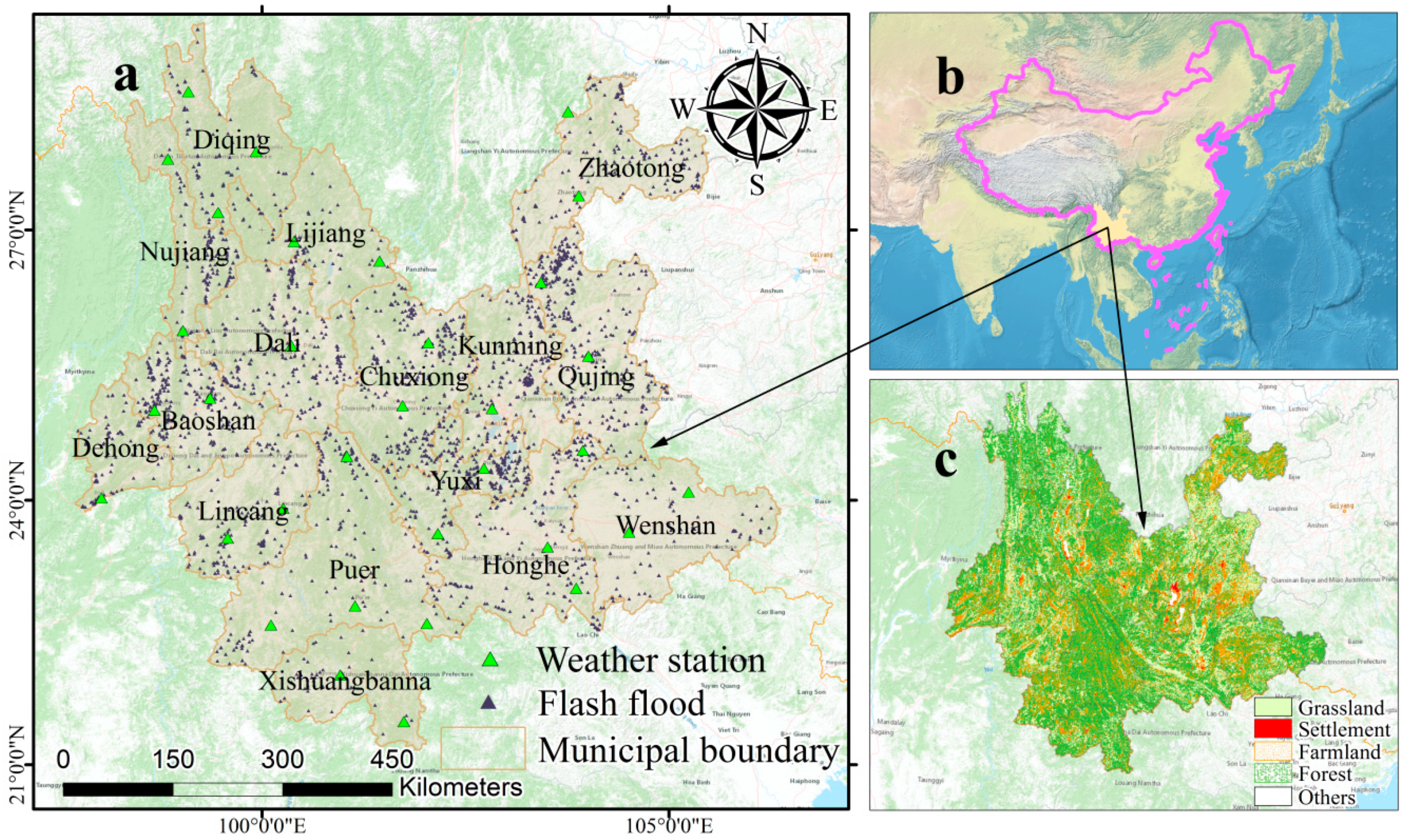
2.1. Study Area

Yunnan Province (21°–29° N, 97°–106° E) is located in southwestern China and is situated on the eastern edge of the collision zone between the Eurasian and Indian continental plates. This region is characterized by some of the most complicated and neotectonic activity and tectonic movements on the Chinese mainland (Figure 1) [34]. Yunnan follows the spatial extent of the land area for this region and covers roughly 394,100 km²; the population was 47.7 million at the end of 2016 (http://www.yn.gov.cn/yn_yngk/gsgk/index.html). Economic activities are gradually gaining momentum, and the yearly economy has exceeded 1.63 trillion yuan (RMB; http://www.stats.gov.cn/) since 2017 in Yunnan. Although Yunnan’s economy has made significant progress, the level of urbanization remains lows, and the township density is relatively sparse [35]. Yunnan is located in the Yunnan–Guizhou Plateau; and most of the areas are dominated by high mountains, deep valleys, and dense mountain streams where vertical differentiation in heat and water occurs as a result of changes in landform and altitude [36]. In addition, the precipitation in northwestern and central Yunnan has increased in recent years [37]. All of these conditions have contributed to making this study area one of the most geophysical hazard-prone regions in China.

2.2. Selection and Pretreatment of Data

The flash flood data used in this research are from the National Flash Flood Investigation and Evaluation Project, which was launched in 2013 to research the historical flash floods that occurred from 1949 to 2015 on a national scale, and the disaster areas were assumed as a point for collection [29]. In Yunnan, the number of flash floods was 3166, which we derived from the above-mentioned project. Current research has shown that the occurrence of flash flood is closely related to precipitation, topography, and human influence [14,21,29]. To explore the relationship between flash floods and the driving factors of flash floods, we selected the following factors: precipitation factors (unit: mm), elevation (ELE, unit: m), topographic relief (TR, unitless), slope (SLP, unit: °), normalized difference vegetation index (NDVI, unitless), population density (PD, unit: person/km²), and GDP (unit: yuan/km²). The precipitation factors included the 10 min precipitation (M10_20), 60 min precipitation (M60_20), 6 h precipitation (H6_20), and 24 h precipitation (H24_20) in 20-year return period, which reflect the impact of various precipitation intensities on flash floods. In addition, the station data of annual mean precipitation used to calculate the gravity center in Yunnan Province were acquired from the National Weather Service of China (http://www.cma.gov.cn/).

Table 1. Source and resolution of the raw data sets.

Factors	Source
Flash floods	China: Flash Flood Investigation and Evaluation Dataset of China, 1949–2015, 1:50,000, vector data.
Precipitation factors	China: Flash Flood Investigation and Evaluation Dataset of China, vector data.
DEM	China: Geospatial Data Cloud, 2000, 90 m × 90 m, raster data.
Population density	China: Resources and Environmental Sciences Data Center, 2000, 2005,2010, and 2015, 1 km × 1 km, raster data.
GDP	China: Resources and Environmental Sciences Data Center, 1995, 2000, 2005, 2010, and 2015, 1 km × 1 km, raster data.
Normalized difference vegetation index	USA: NASA’s MODIS web site, 2001–2015, 1 km × 1 km, raster data.
Landcover	China: Global Change Research Data Publishing & Repository, 2010, 1 km × 1 km, raster data.

shows the source and resolution of all raw data sets.

In this study, we interpolated precipitation raster data by the Inverse Distance Weighted in ArcGIS10.2 (ESRI, Inc., Redlands, CA, USA), which was based on the vector data of precipitation factors, and the final resolution was 1 km × 1 km. We calculated topographic relief using focal statistics in the ArcGIS 10.2 software, which was represented by elevation standard deviation based on the DEM data; the SLP also was generated by this data.

2.3. Methodology

2.3.1. Temporal Pattern

To explore the temporal pattern of flash floods in Yunnan, we analyzed the characteristics of year and month in this study, wherein we calculated the characteristic of year by the package “changepoint” in R software (R Core Development Team, R Foundation for Statistical Computing, Vienna, Austria), which implements various mainstream and specialized changepoint methods to find single and multiple changepoints within data [38]. The month characteristic was analyzed (from January to December) by the year characteristic.

2.3.2. Spatial Pattern

(1) Kernel density estimation

In this paper, kernel density estimation techniques were used for establishing representations for the flash floods, since the kernel function can regard this estimate as averaging the impact of a kernel function centered at the flash flood point and evaluated at each point. We calculated spatial intensity of the flash floods using a kernel density estimation:

$${\lambda }_h(P)=\frac{1}{nh}{\displaystyle \sum _{i=1}^{n}k\left(\frac{P-P_i}{h}\right)}$$

(1)

where λ_h(P) is the estimated spatial intensity of the flash floods, P₁, ⋯, P_n are the locations of n observed flash floods, k(.) is the kernel, a meristic but not necessarily positive function that unites to one, and h is the bandwidth and determines the radius of a circle centered on P that the flash flood points P_i will contribute to the intensity λ_h(P). We calculated the spatial density of the flash floods to conduct the kernel density estimation in ArcGIS 10.2 and determined the search radius (bandwidth) based on the mean random distance (RD mean) calculations [39].

(2) Spatial mismatch analysis

Spatial mismatch analysis has a profound impact in the economy to measure misbalance between two spatially distributed factors, like unemployment and job distribution etc. In this study, the spatial distribution of number of flash floods in different time periods was taken as the input factor. We used spatial mismatch analysis to measure the imbalance between the number of flash floods in two different time periods. The formula is given as follows [40]:

$$SM{I}_i=\left(\frac{B_i}{{\displaystyle \sum _{i=1}^n{B}_i}}-\frac{F_i}{{\displaystyle \sum _{i=1}^n{F}_i}}\right)\times 100$$

(2)

where SMI_i expresses the spatial balance of city i between the number of the flash floods in two different time periods, F_i and B_i refer to the number of flash floods during start and end time periods. To judge whether the spatial relationship of the number of flash floods in two time periods was balanced, we selected a standard value to assist us by Jenks Natural Breaks Classification, which has a minimum variance sum for each class and indicates that features in the same class are more consistent. We divided the value of SMI_i into six classes: the middle two classes were balanced, and the absolute value of the two classes was less than 1.5. If the absolute value of SMI_i was more than 1.5, it showed that the relationship between the number of flash floods in two different time periods was unbalanced in city i [41].

(3) Standard deviational ellipse

The standard deviational ellipse (SDE) has long served as a general geographic information system tool used to measure bivariate distributed characteristics. The tool typically is used to delineate the geographic distribution trend of features by summarizing both their orientation and dispersion. Since our flash flood data is presented in the form of points, this method can be used to determine the direction and trend. In ArcGIS10.2, the SDE is primarily determined by three elements: average location, dispersion (or concentration), and orientation. In addition, the SDE can be described as one, two, or three standard deviations, which can contain approximately 68%, 95%, or 99% of centroids of all input features, respectively. In this study, we selected one standard deviation [42].

(4) Spatial gravity center model

The spatial gravity center model has the advantage to research the spatial-temporal migrations of factors by analyzing the trajectory of their gravity center. We used the spatial gravity center model visually and accurately to reveal the distribution and evolution characteristics of factors in two-dimensional space [40]. To analyze the change trajectories of flash floods, precipitation, and human activities, we calculated the gravity center coordinates of the flash floods, annual mean precipitation, and population density [43]. The time interval of annual mean precipitation and population data was from 2001 to 2015, and we analyzed flash floods consistent with this interval. The gravity center coordinate of the flash floods is given as follows:

$$G_f(x)=\frac{{\displaystyle \sum _{i=1}^n{f}_i(x)}}{n},G_f(y)=\frac{{\displaystyle \sum _{i=1}^n{f}_i(y)}}{n}$$

(3)

where G_f(x) and G_f(y) show the gravity center coordinate of annual flash floods, n is the annual number of flash floods, and f_i(x) and f_i(y) are the geometric coordinates of i-th flash floods (i = 1, 2,⋯n) [25]. Moreover, the gravity center coordinate of the annual mean precipitation and population density are given as follows:

$$G(x)=\frac{{\displaystyle \sum _{i=1}^n{x}_i\times k_i}}{{\displaystyle \sum _{i=1}^n{k}_i}},G(y)=\frac{{\displaystyle \sum _{i=1}^n{y}_i\times k_i}}{{\displaystyle \sum _{i=1}^n{k}_i}}$$

(4)

where G(x) and G(y) express the yearly gravity center coordinate of the factor (annual mean precipitation or population density), (x_i, y_i) is the geometric coordinate of i-th meteorological station of annual mean precipitation (or municipal administrative unit of population density), and k_i refers to the attribute value of the i-th meteorological station (or municipal administrative unit) [40].

2.3.3. Driving Force Analysis

In this study, we explored the relationship between flash floods and driving factors in subregions of the landcover. These subregions include grassland, settlement, farmland, and forest, as almost all flash floods occurred in these subregions. We generated 1000 random points in each subregion and extracted the values of the driving factors and the results of kernel density estimation for the flash floods at each random point on the spatiotemporal scale. On this basis, correlation and interaction were analyzed.

(1) Pearson correlation coefficient

The Pearson correlation coefficient is a classic mathematical method used to show the correlation between two factors x and y where the value of it ranges between (−1) and (+1). The mathematical formula is given by the following:

$$r=\frac{{\displaystyle {\sum }_{i=1}^n{x}_i{y}_i-\frac{{\displaystyle {\sum }_{i=1}^n{x}_i{\displaystyle {\sum }_{i=1}^n{y}_i}}}{n}}}{\sqrt{\left({\displaystyle {\sum }_{i=1}^n{x}_i^2}-\frac{{\left({\displaystyle {\sum }_{i=1}^n{x}_i}\right)}^2}{n}\right)\left({\displaystyle {\sum }_{i=1}^n{y}_i^2}-\frac{{\left({\displaystyle {\sum }_{i=1}^n{y}_i}\right)}^2}{n}\right)}}$$

(5)

where r is the Pearson correlation coefficient between values x and y, and n refers to the numbers of values x and y. The r values and corresponding correlation levels are shown in

Table 2. Pearson correlation coefficient and corresponding correlation levels.

r Value	Correlation Level
r = 0	no correlation
0 < ∣r∣ < 0.2	very weak correlation
0.2 < ∣r∣ < 0.4	weak correlation
0.4 < ∣r∣ < 0.6	intermediate correlation
0.6 < ∣r∣ < 0.8	strong correlation
0.8 < ∣r∣ < 1	very strong correlation
∣r∣ = l	perfect correlation

[44].

(2) Driving factors interaction on the flash floods

Different factors have different effects on the flash floods, and the same factors have different influence on the flash floods in the different subregions of the landcover. In this paper, many factors were selected to explore the driving force, there may be a correlation between the factors. To avoid the multicollinearity of driving factors and explore the interaction of driving factors on flash floods and understand which factors were dominant in the interaction, we selected principal component analysis and multiple linear regression, which enabled us to summarize and visualize the information in the driving factors.

Principal component analysis is an oldest multivariate technique and it is employed by almost all scientific disciplines. Its goal is to reflect the important information from the original data. Meanwhile, it can transform the multicollinearity of driving factors into a set of linearly independent principal components [45]. Detailed information about the principal component analysis were described by previous researches. We determined the number of principal components by the total variance, which was more than 85% [46]. In addition, we measured the contribution of the variable on the principal component by using the “FactoMineR” R package.

Multiple linear regression model is a statistical tool that can be considered as the course of fitting models to data. It can summarize data as well as investigate the relationship between input variables. In this study, the input variables were the principal components of the output of the principal component analysis. Multivariate linear regression is described in detail in reference to previously published studies [47].

2.3.4. Sensitivity analysis

To assess response of flash floods on economic development, we employed a sensitivity assessment model to calculate the flash floods’ sensitivity to GDP. This method is a quantitative analysis that researches the impacts of changing GDP on the flash floods. The formula is given as follows:

$$S=\frac{\left[\left(F_{t_2}-F_{t_1}\right)/F_{t_1}\right]}{\left[\left(G_{t_2}-G_{t_1}\right)/G_{t_1}\right]}$$

(6)

where S represents the value of sensitivity; F_t1 and F_t2 refer to, respectively, the flash floods at the start and end of the time period; and G_t1 and G_t2 refer to, respectively, GDP at the start and end of the time period. We divided sensitivity into four levels according to the published studies (

Table 3. S value and corresponding sensitivity level.

S Value	Sensitivity Level	Description
S ≤ 0	Non-sensitivity	It indicates the changes in the flash floods and economic development do not have any synchronized characteristics.
0 < S ≤ 10	Low-sensitivity	It indicates the flash floods have low sensitivity to economic development.
10 < S ≤ 20	Mid-sensitivity	It indicates the flash floods have medium sensitivity to economic development.
S > 20	High-sensitivity	It indicates the flash floods have high sensitivity to economic development.

) [40,48].

3. Results

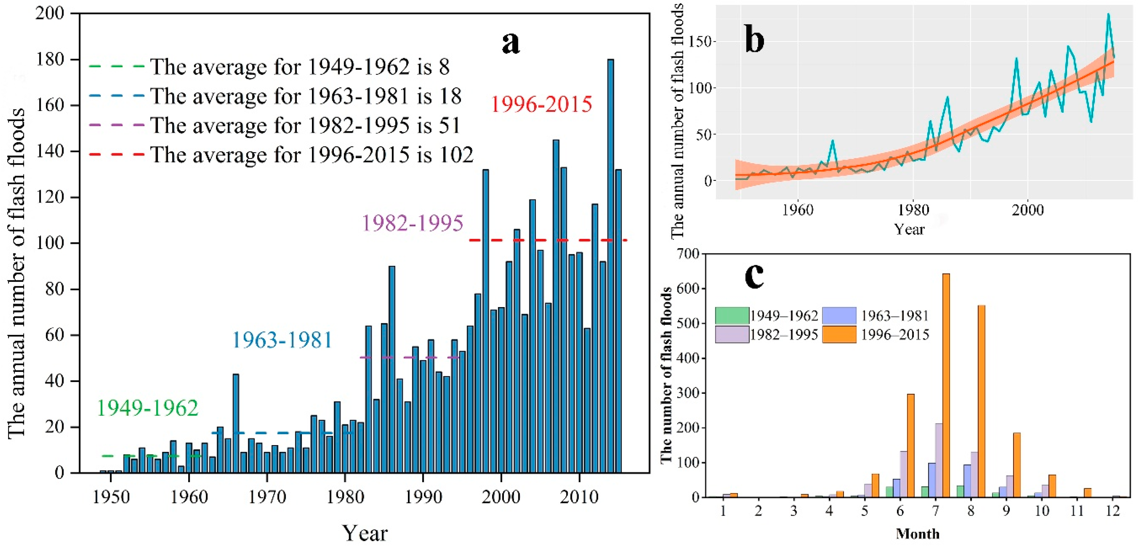
3.1. Temporal Pattern of the Flash Floods

Figure 2 shows the characteristics of the temporal variation of flash floods in Yunnan. The annual flash floods gradually increased from 1949 to 2015 (Figure 2b,

Table 4. The number of flash floods on different time scales.

Year Interval	Year	June	July	August
1949–1962	104	30	31	34
1963–1981	331	53	99	94
1982–1995	704	133	213	131
1996–2015	2027	297	643	552

). On the basis of the descriptions in Section 2.3.1, annual flash floods were divided into four time periods, the number of flash floods was 104, 331, 704, and 2027 during 1949–1962, 1963–1981, 1982–1995, and 1996–2015, respectively (Figure 2a). For the four time periods (1949–1962, 1963–1981, 1982–1995, and 1996–2015), a high level of monthly flash floods occurred in June (30, 53, 133, and 297 flash floods, respectively), July (31, 99, 213, and 643 flash floods, respectively), and August (34, 94, 131, and 552 flash floods, respectively), and no flash floods occurred in February (Figure 2c).

3.2. Spatial Pattern of the Flash Floods

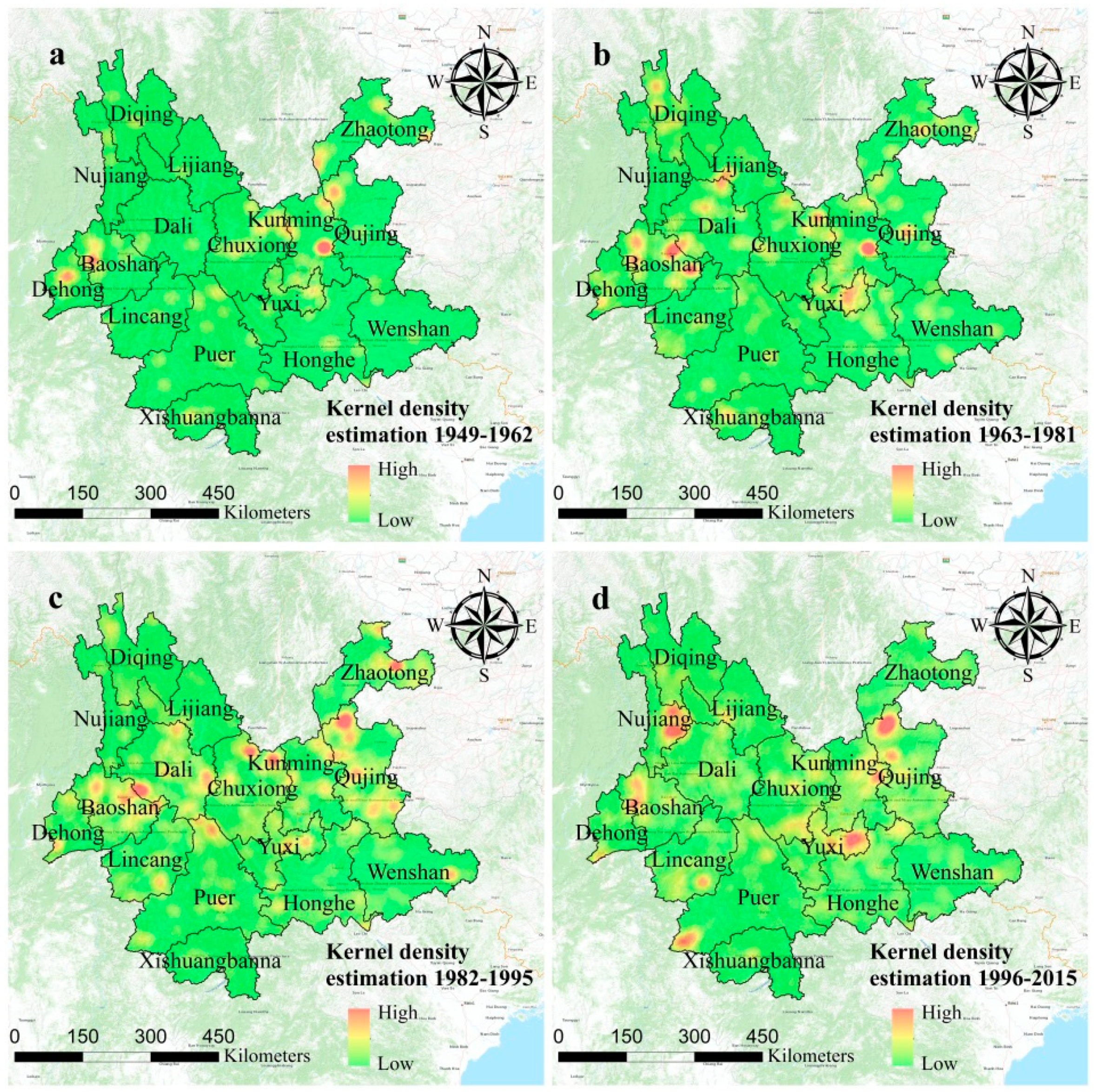
3.2.1. The Result of Kernel Density Estimation

The results of kernel density estimations of flash floods are shown in Figure 3. A relatively high number of flash floods was concentrated in Kunming (18 flash floods), Chuxiong (14 flash floods), Baoshan (10 flash floods), Yuxi (10 flash floods), and Zhaotong (10 flash floods), and the lowest level occurred in Lijiang in 1949–1962 (Figure 3a). In the 1963–1981 period, the most frequent occurrence of flash floods was in Baoshan (47 flash floods); other high-incidence areas included Kunming (32 flash floods), Dali (37 flash floods), and Yuxi (32 flash floods) (Figure 3b). Furthermore, the frequency of the flash floods has increased significantly since the 1982–1995 period. A high frequency of flash floods occurred in Qujing (113 flash floods), Dali (88 flash floods), Chuxiong (74 flash floods), and Baoshan (76 flash floods) in 1982–1995; a low frequency was concentrated in Nujiang (7 flash floods) and Xishuangbanna (6 flash floods) (Figure 3c). In general, the number of the flash floods in Yunnan reached its maximum in the 1996–2015 period. The areas with more than 200 flash floods included Qujing (275 flash floods) and Yuxi (201 flash floods), and the lowest number occurred in Xishuangbanna (30 flash floods) (Figure 3d).

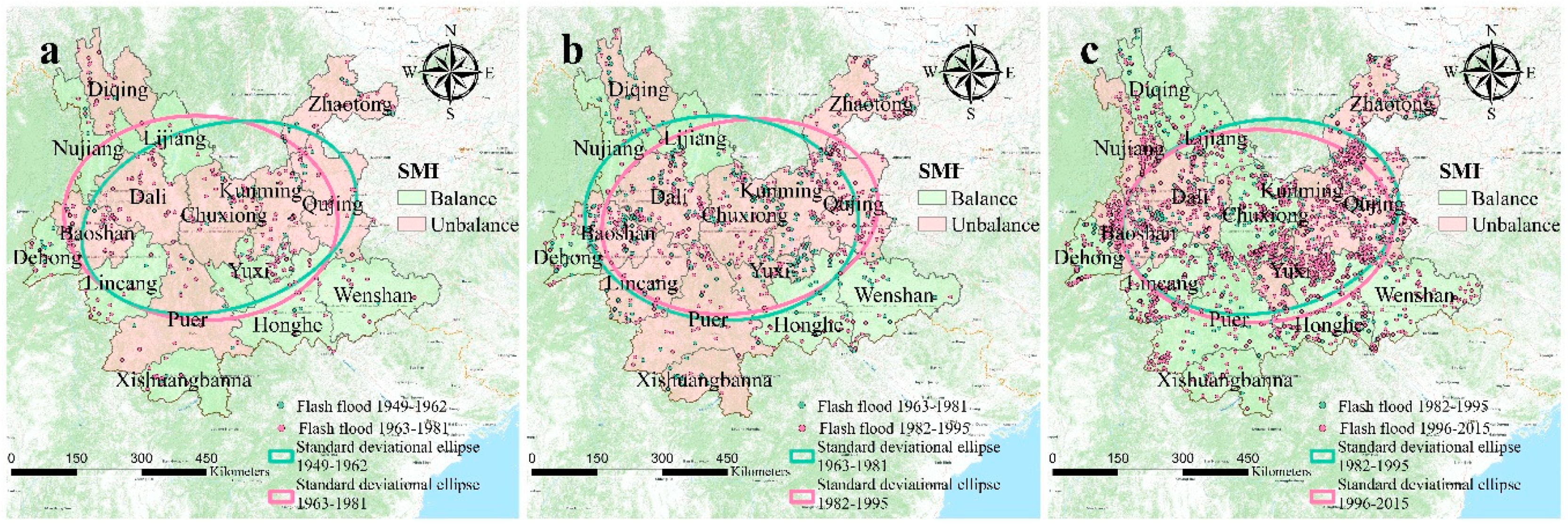
3.2.2. Results of Spatial Mismatch Analysis and SDE

The regions with spatial unbalance were distributed mainly in Zhaotong, Qujing, Kunming, Chuxiong, Puer, Dali, Diqing, and Baoshan from the 1949–1962 to the 1963–1981 time period (Figure 4a). Similarly, standard deviational ellipses showed that the orientation and trends were located in these regions. From the 1963–1981 to the 1982–1995 time periods, the regions with an unbalanced frequency of flash floods had extended to the southern areas, which included Lincang and Xishuangbanna (Figure 4b). Additionally, the orientation and trend of standard deviational ellipses also were located in these areas. Fewer unbalanced areas, however, were evident from the 1982–1995 to the 1996–2015 time periods (Figure 4c), and the flash floods mainly occurred in these unbalanced areas (Zhaotong, Qujing, Kunming, Yuxi, Dali, Nujiang, and Baoshan). Overall, the orientation and trend of standard deviational ellipses were consistent with the unbalanced areas.

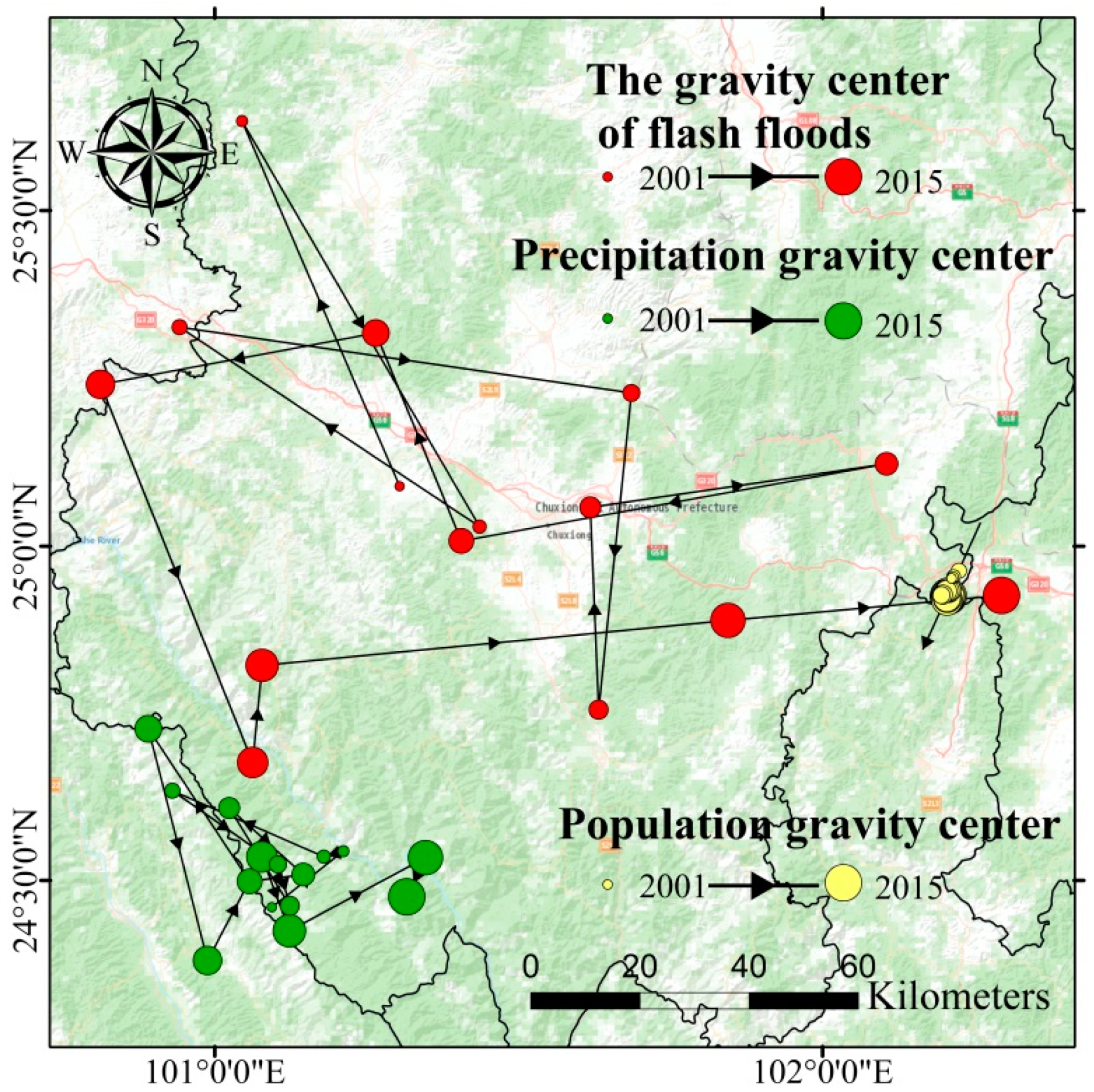
3.2.3. Results of the Spatial Gravity Center Model

As shown in Figure 5, the gravity center of the flash floods was located mainly in Chuxiong, and its change trajectories were random. The gravity center of annual mean precipitation was focused on the border between Chuxiong and Puer, and its change trajectories were also random, but they had some similarity to that of the flash floods. The gravity center of the population moved gradually along the southwest region from 2001 to 2015.

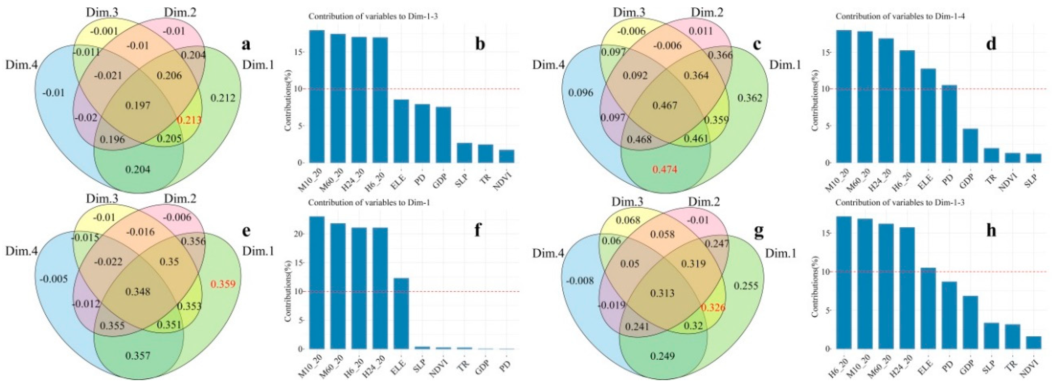
3.3. Driving Factors for the Spatial Distribution of the Flash Floods

We performed a correlation analysis between the flash floods and driving factors in the different subregions of the landcover, as shown in

Table 5. Pearson correlation coefficient (r) between the flash floods and driving factors in the different subregions of the landcover based on Formula (5).

Factors	Grassland		Settlement		Farmland		Forest
	r	P	r	P	r	P	r	P
M10_20	0.487	<0.001	0.675	<0.001	0.445	<0.001	0.466	<0.001
M60_20	0.335	0.001	0.593	<0.001	0.348	0.001	0.326	0.001
H6_20	0.449	<0.001	0.395	<0.001	0.445	<0.001	0.492	<0.001
H24_20	0.501	<0.001	0.519	<0.001	0.381	<0.001	0.485	<0.001
ELE	0.431	<0.001	0.674	<0.001	0.402	<0.001	0.257	0.01
TR	−0.077	0.446	−0.146	0.172	0.219	0.032	−0.014	0.888
SLP	−0.05	0.619	−0.094	0.382	−0.176	0.085	−0.081	0.424
NDVI	−0.241	0.016	0.061	0.571	−0.222	0.029	−0.234	0.02
PD	0.082	0.42	−0.211	0.048	0.108	0.297	−0.098	0.335
GDP	0.098	0.332	0.042	0.697	0.226	0.027	0.233	0.02

. Additionally, we analyzed the interaction of driving factors on the flash floods; the results are presented in Figure 6. In the grassland, the highest r value was the H24_20 (r = 0.501, P < 0.001). Other higher r values included M10_20 (r = 0.487, P < 0.001), H6_20 (r = 0.449, P < 0.001), ELE (r = 0.431, P < 0.001), and M60_20 (r = 0.335, P = 0.001). The highest R² value of multiple linear regression was 0.213, which was based on the principal component (Dim.1, Dim.2, Dim.3, and Dim.4). Driving factors that had a greater contribution included M10_20 (17.91%), M60_20 (17.39%), H24_20 (16.99%), and H6_20 (16.93%). Regarding the settlement, the higher r values of driving factors exhibited the following ranking: M10_20 (r = 0.675, P < 0.001) > ELE (r = 0.674, P < 0.001) > M60_20 (r = 0.593, P < 0.001) > H24_20 (r = 0.519, P < 0.001) > H6_20 (r = 0.395, P < 0.001). The interaction of Dim.1 and Dim.4 contributed the highest R² value, which were controlled mainly by the M10_20 (17.95%), M60_20 (17.79%), H24_20 (16.84%), H6_20 (15.21%), ELE (12.73%), and PD (10.49%). Regarding the farmland, M10_20, H6_20, ELE, H24_20, and M60_20 were the most important driving factors, with r values of 0.445 (P < 0.001), 0.445 (P < 0.001), 0.402 (P < 0.001), 0.381 (P < 0.001), and 0.348 (P = 0.001), respectively. The highest R² value occurred in Dim.1, and the main contributing factors were M10_20 (23.01%), M60_20 (21.81%), H6_20 (21.07%), H24_20 (21.06%), and ELE (12.28%). The characteristics of forest were similar to those of the other three subregions. The higher r values included H6_20 (r = 0.492, P < 0.001), H24_20 (r = 0.485, P < 0.001), M10_20 (r = 0.466, P < 0.001), and M60_20 (r = 0.326, P = 0.001). In addition, the highest R² was determined by the interaction of Dim.1 and Dim.3, and H6_20 (17.14%), M10_20 (16.83%), M60_20 (16.19%), H24_20 (15.72%), and ELE (10.48%) were dominant.

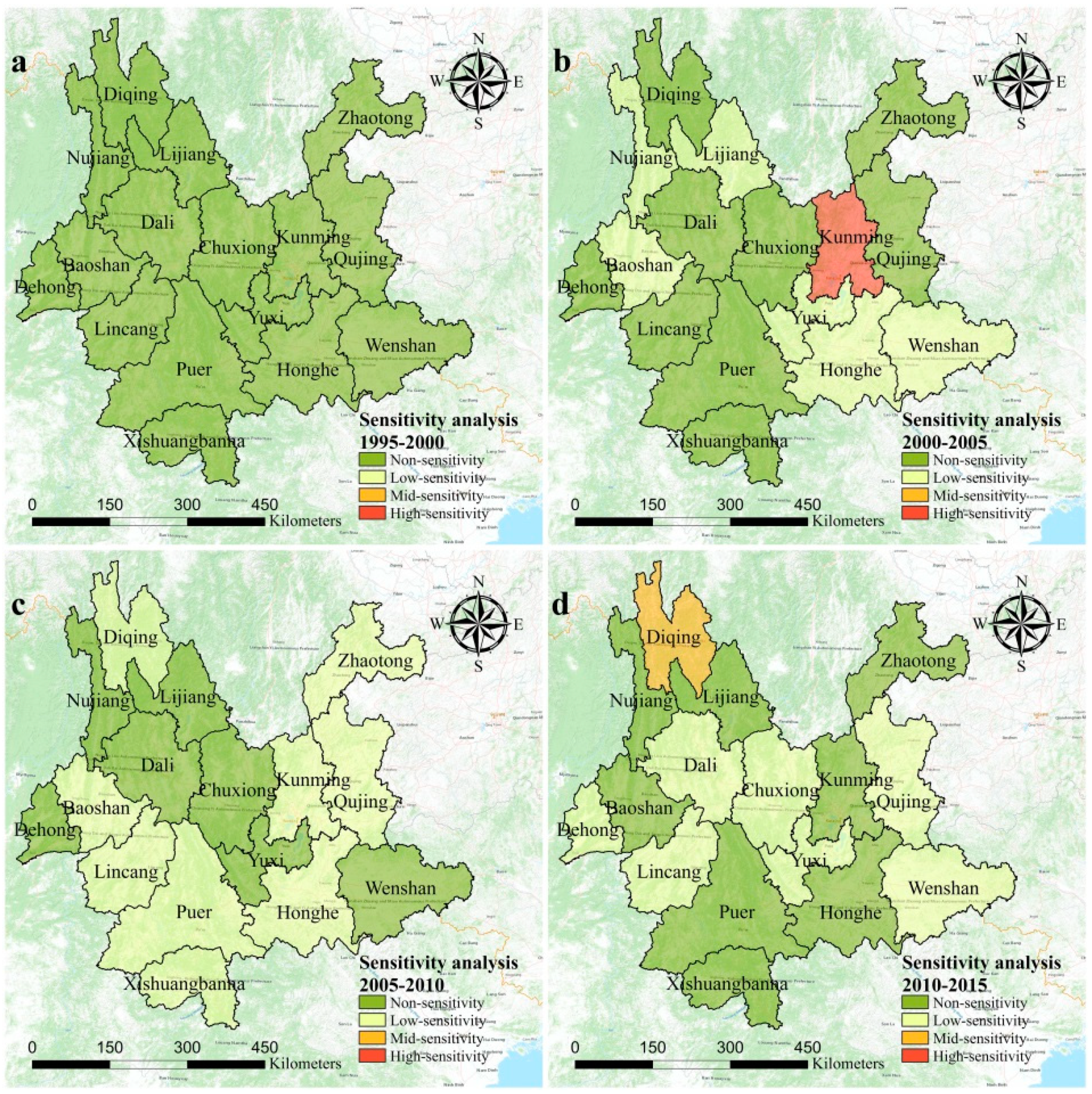
3.4. Sensitivity Analysis between the Flash Floods and Economy Development

By combining the data of the flash floods and GDP and using Formula (6), we calculated the value of sensitivity (S) of the flash floods to the economic development of each city in Yunnan Province, as shown in Figure 7. From an overall perspective, fewer regions experienced medium and high sensitivity during the study period, and the quantity of regions without sensitivity first decreased and then remained stable. During 1995–2000, all regions were non-sensitive. In comparison, the quantity of low-sensitivity regions during 2000–2005 and 2005–2010 increased to six (Nujiang, Baoshan, Lijiang, Yuxi, Honghe, and Wenshan) and nine (Zhaotong, Qujing, Kunming, Honghe, Xishuangbanna, Puer, Lincang, Baoshan, and Diqing), respectively. Simultaneously, Kunming was the highest sensitivity region (S = 21.86) and low-sensitivity (S = 0.98) during these two periods. In the 2010–2015 time period, the flash floods in half of the regions were not sensitive to GDP in Yunnan Province, whereas Diqing was the mid-sensitivity region (S = 10.67).

4. Discussion

4.1. Temporal and Spatial Distribution of the Flash Floods

In this study, a significant variation occurred in the annual and monthly quantity of the flash floods on a provincial scale (Figure 2). The annual quantity gradually increased from 1949 to 2015. The probable causes included human activity and the heavy precipitation that has become more frequent over these years [49,50]. However, the possible reason why flash floods were rare in the 1950s is that many flash floods were not recorded in the early years of the founding of the People’s Republic of China. In addition, our finding revealed that the most frequent quantity of flash floods occurred during 1996–2015, and the average quantity of flash floods was 102 per year. This result showed that, in general, a similar trend occurred in China, which has been supported by existing studies [25,29]. In the meantime, Yangtze River Basin floods have triggered multiple flash floods, which can be explained by the fact that economic development achieved through reform and opening-up has damaged the environment [21]. Regarding monthly variations, flash floods have been concentrated in June, July, and August. The finding was further evidence of the effects of precipitation on flash floods, because heavy precipitation mainly occurred in these three months [51].

The kernel density estimation, unbalanced regions, standard deviational ellipse, and gravity centers showed that flash floods were mainly concentrated in Baoshan, Dali, Chuxiong, Kunming, Yuxi, Qujing, and Zhaotong (Figure 3 and Figure 4). This high concentration of flash floods may have been caused by the elevated levels of precipitation in the central and western regions of Yunnan Province, which have played an important role as external factors [52]. The formation of flash floods was affected by precipitation, environmental background conditions, and human activities, etc. Of the above-mentioned regions, environmental background condition and human activities were other important influencing factors, with the exception of precipitation. In Yunnan, most of the regions are predominately mountainous landscapes [53], which provided ideal geographical conditions for the formation of flash floods. Additionally, the urban agglomerations and major economic area are located in the central regions of Yunnan [54], which leads to the proliferation of environmental destruction, which was another important reason for the formation of flash floods in these regions. Furthermore, previous researchers have investigated the species distribution in Yunnan, their study have revealed low-species areas that were consistent with the high-incidence regions of flash floods [55]; these areas have a high density of human activity, which leads to the destruction of hydrological processes, thus providing conditions for the occurrence of flash floods. According to the results of the change trajectories of gravity centers (Figure 5), the trajectories of flash floods were somewhat similar to those for precipitation but not for population. This finding can be explained by the existing research. Liu et al., for example, found that the influence of precipitation on the flash floods was greater than that of human activities over the short term (i.e., during the 15-year period from 2001 to 2015) [25].

4.2. Driving Factors Influencing the Flash Floods in Yunnan Province

Our findings showed that precipitation and ELE were the main factors affecting flash floods from 2001 to 2015 (Table 5 and Figure 6). This result indicated that flash floods might be easily induced in high-altitude areas by heavy precipitation, and vegetation cover was negatively correlated with flash floods in grassland (r = −0.241, P = 0.016), farmland (r = −0.222, P = 0.029), and forest (r = −0.234, P = 0.02), which is consistent with existing studies [5,21,29]. Regarding the different subregions of the landcover, the driving factors revealed different effects on flash floods. In the grassland, the H24_20 had the maximum correlation with the flash floods, but the ELE did not exceed the average contribution rate for the interaction of driving factors. This is because the topographic relief of the grassland was relatively small. Additionally, the economic activities were not obvious [56], and the short periods of heavy precipitation did not produce strong scour. In this surrounding, the TR, SLP, PD, and GDP had less influence on flash floods (Table 5). In comparison, the contribution rate of ELE and PD exceeded the average value for the interaction of driving factors in settlement. As the population increased, the economic activities expanded to the high altitude area and the ecological system was damaged, which determined the elevation and human activities had a certain boost on flash floods [57]. In contrast, the TR, SLP, and NDVI showed a pretty low correlation to flash floods, which likely occurred because the topographic relief, slope, and vegetation coverage held to a relatively low level in the settlement [58]. This subregion was dominated by small basins and presented the most relevant relationship between flash floods and M10_20. Such a relationship was consistent with the short duration precipitation, which could cause flooding in small basins that have a low time of concentration. For the farmland, the TR and SLP had a greater effect on flash floods than on other subregions (Table 5). This topographic relief and slope mainly included the lower hilly areas of the farmland, which had a higher population density and greater influence on the formation of the flash floods [29,59]. Regarding the forest, GDP had a higher correlation to flash floods than other subregions (Table 5). A possible reason for this correlation was that economic development led to the destruction of forests [60]; we can draw a similar conclusion from the effects of NDVI on flash floods.

4.3. Sensitivity Analysis of the Flash Floods to Economic Development

The sensitivity analysis of the flash floods to GDP is important for sustainable socioeconomic development. The phenomenon of sensitivity rising can influence many development issues, including an imbalance in regional structures and tourism damage [61,62]. The results of our sensitivity analysis showed that all regions were non-sensitive during 1995–2000 (Figure 7a). The early stage of the reform and opening-up of China’s western region was relatively hysteretic for economic development; the intensity of human activity was maintained at a low level and the ecosystem structure was relatively complete [63], which determined this non-sensitivity pattern. During 2000–2005, however, the regions with low-sensitivity increased significantly, and Kunming was the most sensitive area (Figure 7b). In this period, the Development of the West Region, a significant plan for western development launched in 2000, saw economic development in the western city, which was promoted through a massive investment of national capital [64]. Consequently, the quantity of regions with low-sensitivity increased gradually. As the economic and cultural center in Yunnan, Kunming had the strongest human activity [65], which led to the highest sensitivity occurring in this region. With the management of mineral resources in Yunnan Province and regulations to restore farmland to forest, the sensitivity of flash floods to economic development obviously decreased in Kunming during 2005–2010. The quantity of regions with low-sensitivity increased gradually in this period, which can be explained primarily by the macroscopic development of the area [66]. Subsequently, more attention was paid to ecological protection and harmonious economic development, including primary functional area planning (2011) and national new urbanization planning (2014) [60], which determined that the sensitivity of flash floods to economic development decreased gradually during 2010–2015.

To prevent and control flash floods, we need to not only control human activities, such as excessive deforestation and mining, but also implement harmonious economic development and protect the integrity of ecosystem. Regarding the high-incidence areas of flash floods, the rational use of land and flexible barriers should be utilized in these regions. In addition, the government should strengthen its ability to predict flash floods during heavy periods of precipitation.

Our study shows that precipitation and elevation in settlement have a significant impact on flash floods than in other subregions. This result reveals the potential impact of human activities on the environment. Similarly, partition research should be considered when studying the relationship between flash floods and driving forces in other parts of the world, as the flash floods differ in background conditions in different subregions of landcover. However, the study has some drawbacks, including, for example, the time series of driving factors did not begin in 1949. In the future, a longer time series of data can be performed. Precipitation data interpolation should consider mountain terrain in order to reflect the change of climate with elevation. In addition, the spatial analysis methods used in this paper included the kernel density estimation, spatial mismatch analysis, standard deviational ellipse, and spatial gravity center model, which can highlight the spatial distribution characteristics of flash floods on a large regional scale, but have a weak application effect on small regions (e.g., flood protection works, excessive human exposure within the floodplain, basin shape, local geomorphology, and others). As to the principal component analysis, the method to determine the number of principal components has not been unified, which may lead to the loss of local information.

5. Conclusions

In this study, we examined the temporal and spatial distribution of flash floods; the driving factors for the spatial distribution of the flash floods in different subregions of the landcover; and the sensitivity (S) of flash floods to economic development using the changepoint, kernel density estimation, spatial mismatch analysis, standard deviational ellipse, spatial gravity center model, Pearson’s correlation coefficient, multiple linear regression, principal component analysis, and sensitivity analysis. Yunnan Province, in southwestern China, was selected as the study region because of the high incidence area of flash floods and its representative major mountainous landform. The temporal variation of the flash floods showed that the annual quantity of flash floods gradually increased from 1949 to 2015, and the months with the greatest quantity of flash floods were June, July, and August. As to spatial patterns, the regions with a high quantity of flash floods included Zhaotong, Qujing, Kunming, Yuxi, Chuxiong, Dali, and Baoshan. Furthermore, an analysis of the driving factors for flash floods in different subregions of the landcover showed that precipitation and ELE were the main factors from 2001 to 2015. In the settlement, precipitation and ELE had a greater effect on flash floods than in other subregions. Finally, the spatial–temporal variation of sensitivity revealed that the quantity of regions with non-sensitivity first decreased and then remained stable (from 1995 to 2015). During 2000–2005, Kunming had the highest sensitivity; then, this sensitivity gradually began to weaken.

On the basis of the results of this study, the most effective measure is early warning preferential to heavy precipitation events in the short term. In the long term, we should control human activities and reduce the ecosystem vulnerability caused by damage to species and to vegetation and by population growth to effectively prevent flash floods. According to the sensitivity of flash floods to economic development, Yunnan Province should take note of the previous lessons of imbalance and continue to introduce a balanced development policy.

References

1. Gascón, E.; Laviola, S.; Merino, A.; Miglietta, M.M. Analysis of a localized flash-flood event over the central Mediterranean. Atmos. Res. 2016, 182, 256–268. [Google Scholar] [CrossRef]
2. Rahman, M.T.; Aldosary, A.S.; Nahiduzzaman, K.M.; Reza, I. Vulnerability of flash flooding in Riyadh, Saudi Arabia. Nat. Hazards 2016, 84, 1807–1830. [Google Scholar] [CrossRef]
3. Lian, J.; Yang, W.; Xu, K.; Ma, C. Flash flood vulnerability assessment for small catchments with a material flow approach. Nat. Hazards 2017, 88, 699–719. [Google Scholar] [CrossRef]
4. Ashley, S.T.; Ashley, W.S. Flood Fatalities in the United States. J. Appl. Meteorol. Clim. 2008, 47, 805–818. [Google Scholar] [CrossRef]
5. He, B.; Huang, X.; Ma, M.; Chang, Q.; Tu, Y.; Li, Q.; Zhang, K.; Hong, Y. Analysis of flash flood disaster characteristics in China from 2011 to 2015. Nat. Hazards 2017, 90, 407–420. [Google Scholar] [CrossRef]
6. Gourley, J.J.; Flamig, Z.L.; Vergara, H.; Kirstetter, P.-E.; Clark, R.A.; Argyle, E.; Arthur, A.; Martinaitis, S.; Terti, G.; Erlingis, J.M.; et al. The FLASH project: Improving the tools for flash flood monitoring and prediction across the United States. Bull. Am. Meteorol. Soc. 2017, 98, 361–372. [Google Scholar] [CrossRef]
7. Barredo, J.I. Major flood disasters in Europe: 1950–2005. Nat. Hazards 2006, 42, 125–148. [Google Scholar] [CrossRef]
8. Pereira, S.; Diakakis, M.; Deligiannakis, G.; Zêzere, J.L. Comparing flood mortality in Portugal and Greece (Western and Eastern Mediterranean). Int. J. Disaster Risk Reduct. 2017, 22, 147–157. [Google Scholar] [CrossRef]
9. Xu, J.; Wilkes, A. Biodiversity impact analysis in northwest Yunnan, southwest China. Biodivers. Conserv. 2004, 13, 959–983. [Google Scholar] [CrossRef]
10. Zeng, Z.; Tang, G.; Long, D.; Zeng, C.; Ma, M.; Hong, Y.; Xu, H.; Xu, J. A cascading flash flood guidance system: Development and application in Yunnan Province, China. Nat. Hazards 2016, 84, 2071–2093. [Google Scholar] [CrossRef]
11. Bajabaa, S.; Masoud, M.; Al-Amri, N. Flash flood hazard mapping based on quantitative hydrology, geomorphology and GIS techniques (case study of Wadi Al Lith, Saudi Arabia). Arab. J. Geosci. 2013, 7, 2469–2481. [Google Scholar] [CrossRef]
12. Shi, P.; Lili, L.; Wang, M.; Wang, J.; Chen, W. Disaster system: Disaster cluster, disaster chain and disaster compound. J. Nat. Disasters 2014, 23, 1–12. [Google Scholar]
13. Zhong, D.; Xie, H.; Wei, F.; Liu, H.; Tang, J. Discussion on Mountain Hazards Chain. J. Mt. Sci. 2013, 31, 314–326. [Google Scholar]
14. Xiong, J.; Wei, F.; Liu, Z. Hazard assessment of debris flow in Sichuan Province. J. Geo-Inf. Sci. 2017, 19, 1604–1612. [Google Scholar]
15. Zeleňáková, M.; Gaňová, L.; Purcz, P.; Satrapa, L. Methodology of flood risk assessment from flash floods based on hazard and vulnerability of the river basin. Nat. Hazards 2015, 79, 2055–2071. [Google Scholar] [CrossRef]
16. Guo, E.; Zhang, J.; Ren, X.; Zhang, Q.; Sun, Z. Integrated risk assessment of flood disaster based on improved set pair analysis and the variable fuzzy set theory in central Liaoning Province, China. Nat. Hazards 2014, 74, 947–965. [Google Scholar] [CrossRef]
17. Sangati, M.; Borga, M. Influence of rainfall spatial resolution on flash flood modelling. Nat. Hazards Earth Syst. Sci. 2009, 9, 575–584. [Google Scholar] [CrossRef] [Green Version]
18. Lin, Z.; Nimaji; Huang, Z. Hydrological dynamics simulation and critical rainfall for flash flood in southeastern Tibet. Bull. Soil Water Conserv. 2017, 37, 183–187. [Google Scholar]
19. Jun, D.U.; Wen-Feng, D.; Hong-Yu, R. Relationships between different types of flash flood disasters and their main impact factors in the Sichuan Province. Resour. Environ. Yangtze Basin 2015, 24, 1977–1983. [Google Scholar]
20. Wan, S.; Zhao, N.; Wei, D. Correlation and multi-timescale characteristics of strong precipitations and landslide debris flows in Yunnan Province. J. Catastrophol. 2015, 30, 45–50. [Google Scholar]
21. Xiong, J.; Zhao, Y.; Cheng, W.; Guoliang; Wang, N.; Li, W. Temporal and spatial variation rule and influencing ractors of flash floods in Sichuan Province. J. Geo-Inf. Sci. 2018, 20, 1443–1456. [Google Scholar]
22. Chen, C.-C.; Tseng, C.-Y.; Dong, J.-J. New entropy-based method for variables selection and its application to the debris-flow hazard assessment. Eng. Geol. 2007, 94, 19–26. [Google Scholar] [CrossRef] [Green Version]
23. Tang, C.; van Asch, T.W.; Chang, M.; Chen, G.Q.; Zhao, X.H.; Huang, X.C. Catastrophic debris flows on 13 August 2010 in the Qingping area, southwestern China: The combined effects of a strong earthquake and subsequent rainstorms. Geomorphology 2012, 139, 559–576. [Google Scholar] [CrossRef]
24. Vennari, C.; Parise, M.; Santangelo, N.; Santo, A. A database on flash flood events in Campania, southern Italy, with an evaluation of their spatial and temporal distribution. Nat. Hazards Earth Syst. Sci. 2016, 16, 2485–2500. [Google Scholar] [CrossRef] [Green Version]
25. Liu, Y.; Yang, Z.; Huang, Y.; Liu, C. Spatiotemporal evolution and driving factors of China’s flash flood disasters since 1949. Sci. China Earth Sci. 2018, 61, 1804–1817. [Google Scholar] [CrossRef]
26. Jun, D.U.; Ren, H.; Zhang, P.; Zhang, C. Comparative study of the hazard assessment of mountain torrent disasters in macro scale. J. Catastrophol. 2016, 31, 66–72. [Google Scholar]
27. Rozalis, S.; Morin, E.; Yair, Y.; Price, C. Flash flood prediction using an uncalibrated hydrological model and radar rainfall data in a Mediterranean watershed under changing hydrological conditions. J. Hydrol. 2010, 394, 245–255. [Google Scholar] [CrossRef]
28. Doocy, S.; Daniels, A.; Murray, S.; Kirsch, T.D. The human impact of floods: A historical review of events 1980-2009 and systematic literature review. PLoS Curr. Disasters 2013, 5, 1808–1815. [Google Scholar] [CrossRef] [PubMed]
29. Liu, Y.; Yuan, X.; Guo, L.; Huang, Y.; Zhang, X. Driving force analysis of the temporal and spatial distribution of flash floods in Sichuan Province. Sustainability 2017, 9, 1527. [Google Scholar] [CrossRef]
30. Wang, J.; Xu, C. Geodetector: Principle and prospective. Acta Geogr. Sin. 2017, 72, 116–134. [Google Scholar]
31. Zhou, L.; Zhou, C.; Yang, F.; Wang, B.; Sun, D. Spatio-temporal evolution and the influencing factors of PM2.5 in China between 2000 and 2011. Acta Ecol. Sin. 2017, 72, 161–174. [Google Scholar]
32. Shi, J.; Li, B.; Li, P.; Huang, J.; Sun, F.; Liu, B. Analisis of characteristics and formation mechanism for the 9·17 giant debris flow in Yuanmou Country, Yunnan Province. Geol. Rev. 2018, 64, 665–673. [Google Scholar]
33. Xu, S.; Yuan, Z.; Yang, Z. Based on EKC analysis of landslide and debris flow disasters. Soil Water Conserv. China 2015, 54–56. [Google Scholar]
34. Zhan, W.; Li, F.; Hao, W.; Yan, J. Regional characteristics and influnencing factors of seasonal vertical crustal motions in Yunnan, China. Geophys. J. Int. 2017, 210, 1295–1304. [Google Scholar] [CrossRef]
35. Yang, Y.; Jia, W. Types and geographical environment elements of township placenames in Yunnan Province. Geogr. Res. 2016, 4, 60. [Google Scholar]
36. Cao, X.; Pan, W.; Zhou, S.; Han, Z.; Han, T.; Shui, Z. Seasonal variability of oxygen and hydrogen isotopes in a wetland system of the Yunnan-Guizhou Plateau, southwest China: A quantitative assessment of groundwater inflow fluxes. Hydrogeol. J. 2017, 26, 1–17. [Google Scholar] [CrossRef]
37. Liu, Y.; Zhao, E.; Huang, W.; Zhou, J.; Ju, J. Characteristic analysis of precipitation and temperature change trend in Yunnan in recent 46 years. J. Catastrophol. 2010, 25, 39–44. [Google Scholar]
38. Killick, R.; Fearnhead, P.; Eckley, I.A. Optimal Detection of Changepoints With a Linear Computational Cost. J. Am. Stat. Assoc. 2012, 107, 1590–1598. [Google Scholar] [CrossRef]
39. Guo, F.; Innes, J.L.; Wang, G.; Ma, X.; Sun, L.; Hu, H.; Su, Z. Historic distribution and driving factors of human-caused fires in the Chinese boreal forest between 1972 and 2005. J. Plant Ecol. 2015, 8, 480–490. [Google Scholar] [CrossRef]
40. Chai, J.; Wang, Z.; Yang, J.; Zhang, L. Analysis for spatial-temporal changes of grain production and farmland resource: Evidence from Hubei Province, central China. J. Clean. Prod. 2019, 207, 474–482. [Google Scholar] [CrossRef]
41. Li, T.; Long, H.; Zhang, Y.; Tu, S.; Ge, D.; Li, Y.; Hu, B. Analysis of the spatial mismatch of grain production and farmland resources in China based on the potential crop rotation system. Land Use Policy 2017, 60, 26–36. [Google Scholar] [CrossRef]
42. Wang, B.; Shi, W.; Miao, Z. Confidence analysis of standard deviational ellipse and its extension into higher dimensional euclidean space. PLoS ONE 2015, 10, e0118537. [Google Scholar] [CrossRef]
43. Li, M.; Ren, X.; Zhou, L.; Zhang, F. Spatial mismatch between pollutant emission and environmental quality in China—A case study of NOx. Atmos. Pollut. Res. 2016, 7, 294–302. [Google Scholar] [CrossRef]
44. Irhoumah, M.; Pusca, R.; Lefèvre, E.; Mercier, D.; Romary, R. Diagnosis of induction machines using external magnetic field and correlation coefficient 2017. In Proceedings of the 2017 IEEE 11th International Symposium on Diagnostics for Electrical Machines, Power Electronics and Drives (SDEMPED), Tinos, Greece, 29 August–1 September 2017; pp. 531–536. [Google Scholar]
45. Wang, H.; Zhang, B.; Liu, Y.; Liu, Y.; Xu, S.; Deng, Y.; Zhao, Y.; Chen, Y.; Hong, S. Multi-dimensional analysis of urban expansion patterns and their driving forces based on the center of gravity-GTWR model: Acase study of the Beijing-Tianjin-Hebei urban agglomeration. Acta Geogr. Sin. 2018, 73, 1076–1092. [Google Scholar]
46. Abdi, H.; Williams, L.J. Principal component analysis. Wiley Interdiscip. Rev. Comput. Stat. 2010, 2, 433–459. [Google Scholar] [CrossRef]
47. Khademi, F.; Akbari, M.; Jamal, S.M.; Nikoo, M. Multiple linear regression, artificial neural network, and fuzzy logic prediction of 28 days compressive strength of concrete. Front. Struct. Civ. Eng. 2017, 11, 90–99. [Google Scholar] [CrossRef]
48. Han, Z.; Song, W.; Deng, X. Responses of ecosystem service to land use change in Qinghai Province. Energies 2016, 9, 303. [Google Scholar] [CrossRef]
49. Yu, W.; Shao, M.; Ren, M.; Zhou, H.; Jiang, Z.; Li, D. Analysis on spatial and temporal characteristics drought of Yunnan Province. Acta Ecol. Sin. 2013, 33, 317–324. [Google Scholar] [CrossRef]
50. Liu, L.; Xu, Z.X. Regionalization of precipitation and the spatiotemporal distribution of extreme precipitation in southwestern China. Nat. Hazards 2015, 80, 1195–1211. [Google Scholar] [CrossRef]
51. Liu, J.; Li, L.; Li, J.; Wang, Z.; Chen, S.; Zhang, K. Characteristics of precipitation variation and potential drought-flood regional responses in Yunnan Province from 1954 to 2014. J. Geo-Inf. Sci. 2016, 18, 1077–1086. [Google Scholar]
52. Tao, Y.; He, Q. The temporal and spatial distribution of precipitation over Yunnan province and its response to global warming. J. Yunnan Univ. 2008, 30, 587–595. [Google Scholar]
53. Luo, J.; Zhan, J.; Lin, Y.; Zhao, C. An equilibrium analysis of the land use structure in the Yunnan Province, China. Front. Earth Sci. 2014, 8, 393–404. [Google Scholar] [CrossRef]
54. Liu, X.; Salmeron, D.; Luo, Q.; Rana, S.; Liu, Z. Research on optimal development pattern of Yunnan central economic region. China City Plan. Rev. 2012, 21, 38–45. [Google Scholar]
55. Zhang, M.; Zhou, Z.; Chen, W.; Slik, J.W.F.; Cannon, C.H.; Raes, N. Using species distribution modeling to improve conservation and land use planning of Yunnan, China. Boil. Conserv. 2012, 153, 257–264. [Google Scholar] [CrossRef]
56. Han, Z.; Song, W.; Deng, X.; Xu, X. Grassland ecosystem responses to climate change and human activities within the Three-River Headwaters region of China. Sci. Rep. 2018, 8, 9079. [Google Scholar] [CrossRef] [PubMed]
57. Špitalar, M.; Gourley, J.J.; Lutoff, C.; Kirstetter, P.-E.; Brilly, M.; Carr, N. Analysis of flash flood parameters and human impacts in the US from 2006 to 2012. J. Hydrol. 2014, 519, 863–870. [Google Scholar] [CrossRef]
58. Jenerette, G.D.; Harlan, S.L.; Brazel, A.; Jones, N.; Larsen, L.; Stefanov, W.L. Regional relationships between surface temperature, vegetation, and human settlement in a rapidly urbanizing ecosystem. Landsc. Ecol. 2006, 22, 353–365. [Google Scholar] [CrossRef]
59. Luo, H. Dynamic of vegetation carbon storage of farmland ecosystem in hilly area of central Sichuan Basin during the Last 55 years—A case study of Yanting County, Sichuan Province. J. Nat. Resour. 2009, 24, 251–258. [Google Scholar]
60. Peng, L.; Deng, W.; Zhang, H.; Sun, J.; Xiong, J. Focus on economy or ecology? A three-dimensional trade-off based on ecological carrying capacity in southwest China. Nat. Resour. Model. 2018, 32, e12201. [Google Scholar] [CrossRef]
61. Kourgialas, N.N.; Karatzas, G.P.; Nikolaidis, N.P. Development of a thresholds approach for real-time flash flood prediction in complex geomorphological river basins. Hydrol. Process. 2012, 26, 1478–1494. [Google Scholar] [CrossRef]
62. Chou, J.; Xian, T.; Dong, W.; Xu, Y. Regional temporal and spatial trends in drought and flood disasters in China and assessment of economic losses in recent years. Sustainability 2018, 11, 55. [Google Scholar] [CrossRef]
63. Tang, W.; Zhou, T.; Sun, J.; Li, Y.; Li, W. Accelerated urban expansion in Lhasa City and the implications for sustainable development in a Plateau city. Sustainability 2017, 9, 1499. [Google Scholar] [CrossRef]
64. Yi, S.; Yang, J.; Hu, X. How economic globalization affects urban expansion: An empirical analysis of 30 Chinese provinces for 2000–2010. Qual. Quant. 2016, 50, 1117–1133. [Google Scholar]
65. Hu, S.; Yan, X.; Qu, D.; Li, X. Approach to the legislative problem of the recycling economy in Kunming. Ecol. Econ. 2005, 1, 92–96. [Google Scholar]
66. Gao, J.; Wei, Y.; Chen, W.; Yenneti, K. Urban land expansion and structural change in the Yangtze River Delta, China. Sustainability 2015, 7, 10281–10307. [Google Scholar] [CrossRef]
Figure 1. The study area: (a) the distribution of flash floods in Yunnan Province; (b): the geographical position of Yunnan in China; (c): the different subregions of landcover in Yunnan Province.
Sustainability 11 02926 g001
Figure 2. The characteristics of temporal variation of the flash floods: (a) a histogram of the number of the flash floods per year and the year interval of the flash floods based on changepoint analysis (the green dotted line is 1949–1962, the blue dotted line is 1963–1981, the purple dotted line is 1982–1995, and the red dotted line is 1996–2015); (b) variation trends of annual flash floods. The red line is the fitting line and the dark green line is the change line of the annual number of flash floods; and (c) characteristics of monthly flash floods in different time periods.
Sustainability 11 02926 g002
Figure 3. Kernel density estimation of the flash floods for the four time periods: (a) 1949–1962, (b) 1963–1981, (c) 1982–1995, and (d) 1996–2015.
Sustainability 11 02926 g003
Figure 4. The spatial pattern of spatial mismatch index and standard deviational ellipse at the start and end time periods: (a) from the 1949–1962 to the 1963–1981 time period, (b) from the 1963–1981 to the 1982–1995 time period, and (c) from the 1982–1995 to the 1996–2015 time period. Green dots and standard deviational ellipses indicate the start time period, and red indicates the end time period.
Sustainability 11 02926 g004
Figure 5. Change trajectories of gravity centers of flash floods, annual mean precipitation, and population from 2001 to 2015.
Sustainability 11 02926 g005
Figure 6. Driving factors interaction based on multiple linear regression and principal component analysis for flash floods, and the contribution of driving factors to the principal components (Dim.1, Dim.2, Dim.3, and Dim.4) in the different subregions of the landcover: (a) R2 value of multiple linear regression of principal components to the flash floods in grassland; (b) the contribution of driving factors to Dim.1 and Dim.3 in grassland; (c) R2 value of multiple linear regression of principal components to the flash floods in settlement; (d) the contribution of driving factors to Dim.1 and Dim.4 in settlement; (e) R2 value of multiple linear regression of principal components to the flash floods in farmland; (f) the contribution of driving factors to Dim.1 in farmland; (g) R2 value of multiple linear regression of principal components to the flash floods in forest; and (h) the contribution of driving factors to Dim.1 and Dim.3 in forest. The red number is the highest R2 value. The contribution of driving factors to the principal components greater than the red dotted line indicates that they are dominant.
Sustainability 11 02926 g006
Figure 7. The spatial–temporal variation of sensitivity from 1995 to 2015: (a) during 1995–2000, (b) during 2000–2005, (c) during 2005–2010, and (d) during 2010–2015.
Sustainability 11 02926 g007