Evaluation of Watershed Scale Aquatic Ecosystem Health by SWAT Modeling and Random Forest Technique

Abstract

In this study, we evaluated the aquatic ecosystem health (AEH) with five grades (A; very good to E; very poor) of FAI (Fish Assessment Index), TDI (Trophic Diatom Index), and BMI (Benthic Macroinvertebrate Index) using the results of SWAT (Soil and Water Assessment Tool) stream water temperature (WT) and quality (T-N, T-P, NH₄, NO₃, and PO₄). By applying Random Forest, one of the machine learning algorithms for classification analysis, each AEH index was trained and graded from the SWAT results. For Han river watershed (34,418 km²) in South Korea, the 8 years (2008~2015) observed AEH data of Spring and Fall periods at 86 locations from NAEMP (National Aquatic Ecological Monitoring Program) were used. The AEH was separately trained for Spring (FAI_s, TDI_s, and BMI_s) and Fall (FAI_a, TDI_a, and BMI_a), and the AEH results of Random Forest with SWAT (WT, T-N, T-P, NH₄, NO₃, and PO₄) as input variables showed the accuracy of 0.42, 0.48, 0.62, 0.45, 0.4, and 0.58, respectively. The reason for low accuracy was from the weak strength of the individual trees and high correlation between the trees composing the Random Forest due to the data imbalance. The AEH distribution results showed that the number of Grade A of total FAI, TDI, and BMI were 84, 0, and 158 respectively and they were mostly located at the upstream watersheds. The number of Grade E of total FAI, TDI, and BMI were 4, 50, and 13 and they were shown at downstream watersheds.

1. Introduction

Aquatic ecosystem is defined as a complex community where energy and nutrient exchanges occur through the interaction between living organisms and their environment. A healthy aquatic ecosystem represents a stable and sustainable aquatic environment that maintains its ecological structure, processes, functions, and resilience to stress within its range of natural variability [1]. However, multiple stressors, such as organic and inorganic pollution, land use and geomorphological changes, water extraction, invasive species and pathogens, have detrimental effects on aquatic ecosystems including hydrological, chemical, and biological aspects [2]. There are various evaluation criteria of aquatic ecosystem to decide the practice for water management and restoration on the degraded watershed.

Recently, many biological parameters such as fish, macrophytes, aquatic plants, trophic diatoms, invertebrates have been used to assess the aquatic ecological status [3,4,5,6]. Fish are used as a bioindicator representing the effects of environmental pollution and changes over a long period because it has high mobility and long regeneration time [7]. Macroinvertebrates are sampled easier than other organisms and consist of various species that inhabit from clean to highly polluted water [8,9]. As a source of food for higher trophic level like fish, they have an important role in the nutrient cycle, primary productivity, decomposition, and translocation of materials, and they may imply the past condition due to the relatively low mobility and long-life cycles [10]. Diatoms are used as a bioindicator of stream, because it has characteristics such as diverse species, short life spans, rapid response to changes in stream chemistry and habitat quality, and broadly distribution, which make geographical comparison possible [11,12,13]. For these reasons, they have been used as an important indicator of ecological environments improvement or deterioration.

The Ministry of Environment (MOE) of South Korea has attempted to reflect biological characteristics of aqua-ecology in addition to water quality and have operated the National Aquatic Ecological Monitoring Program (NAEMP) since 2008. The NAEMP assesses a stream’s ecological status including chemical and biological quality of water and environmental characteristics [14]. The monitoring was conducted based on field observation twice a year during spring and fall considering the heavily concentrated precipitation in summer called “Asian monsoon”. It was operated at irregular measuring sites and time frames because patterns of intensive precipitation fluctuated every year [15].

The condition of stream soundness is determined by parameters including nitrogen and phosphorus water quality components, dissolved oxygen (DO), biochemical oxygen demand (BOD), chemical oxygen demand (COD), and temperature. Various models have been developed to produce these stream health characteristics. Among them, Soil and Water Assessment Tool (SWAT) simulates the hydrological and stream water quality considering weather, soil, land management, and agriculture practice of a watershed [16] and has been also used in South Korea by adjusting the parameters to match the characteristics of South Korea [17,18,19]. Although the physico-chemical parameters are related to biological status such as fish, trophic diatom, and invertebrates [20,21,22,23,24], the interrelationship between two parameters are not easy and clear to predict and evaluate the complex aquatic ecosystem by correlation analysis with selected physico-chemical variables. The Random Forest, which is one of the machine learning algorithms, can consider various variables and has good performance by preventing overfitting [25]. In various fields including hydrology, aqua-ecology, environmental remote sensing, Random Forest has been used to predict and evaluate unknown components that are difficult to predict with previous statistical methods [26,27,28,29,30,31,32,33].

The purpose of this study is to confirm the applicability of Random Forest algorithm that consists of SWAT water quality, temperature results and AEH (aquatic ecosystem health) data and to evaluate the AEH for Han river watershed streams.

2. Materials and Methods

2.1. Description of the Study Area

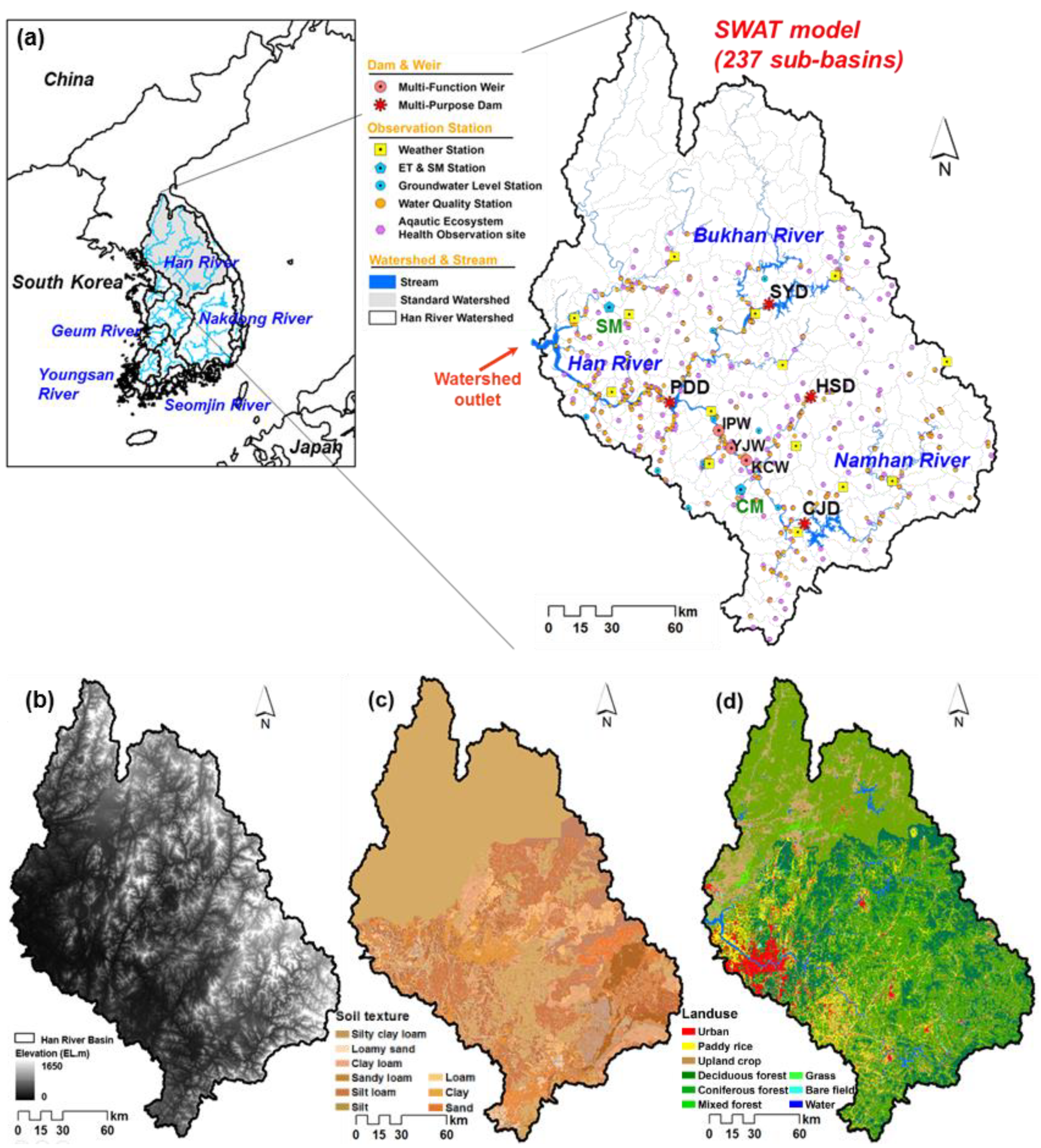
The Han River watershed (34,418 km²) is located in South Korea within the latitudes of 126.24° E to 129.02° E and the longitudes of 36.03° N to 38.55° N. It is the largest watershed in South Korea and occupies approximately a quarter of the country. There are two main rivers, the Bukhan river and the Namhan river, which is joined at the stream where Paldang Dam (PDD) is located and flows to an outlet of the watershed through Seoul metropolitan city. The watershed has three multi-functional weirs (KCW, YJW, and IPW), and three multi-purpose dams (SYD, HSD, and CJD). The multi-functional weirs were constructed in 2012 and total storage of 11 million m³, 13 million m³, and 17 million m³ respectively. SYD and CJD are the largest and second largest in South Korea with a storage capacity of 2.9 billion m³, 2.75 billion m³ and have watershed areas of 2694 km², and 6662 km² respectively. The annual mean precipitation is 1395 mm over 30 years of weather data from 1985 to 2015 and most of the precipitation is concentrated on summer. The seasonal variation of air temperature for spring, summer, fall, and winter is 10.8 °C, 23.6 °C, 12.6 °C, and −2.9 °C respectively. There are 230 water quality observation stations and 313 AEH observation sites (Figure 1a). Figure 1b shows the elevation distribution of the forest zone in the east, decreasing to the west downstream located. Two soil types of 58% sandy loam and 24% loam are dominant (Figure 1c). Land use is composed of 73% forest, 18% agriculture areas (6% rice paddy and 12% upland crops), and 5% urban areas, which are concentrated in the downstream of watershed including Seoul (the capital city of South Korea) (Figure 1d).

2.2. Aquatic Ecosystem Health Index

South Korea has the National Aquatic Ecological Monitoring Program (NAEMP) operated by the National Institute of Environmental Research (NIER) to assess the ecological health of the stream body, which has been in operation since 2008. Based on the direct observations of stream environments, nutrients, and species of organisms, the ecological health has been evaluated using aquatic organism indices such as Fish Assessment Index (FAI), Trophic Diatom Index (TDI), and Benthic Macroinvertebrate Index (BMI) and stream environment indices such as Riparian Vegetation Index (RVI), and Habitat and Riparian Index (HRI) [34]. The program has been operated for the entire country at 1200 sites twice per year, spring (April to June) and fall (August to October). There are 313 monitoring sites located in the Han river watershed. In this study, three indices of FAI, TDI, and BMI pertaining to the aquatic organisms were considered.

Fish refers to organisms at the top level of food chain in water bodies. Using the scores for eight metrics, FAI is calculated from Equation (1) as follows:

$$\mathrm{FAI}=\mathrm{M}1+\mathrm{M}2+\mathrm{M}3+\mathrm{M}4+\mathrm{M}5+\mathrm{M}6+\mathrm{M}7+\mathrm{M}8$$

(1)

where M1 is the total number of domestic species, M2 is the number of riffle benthic species, M3 is number of sensitive species, M4 is population ratio of tolerant species, M5 is population ratio of omnivores, M6 is population ratio of domestic insectivores, M7 is total population of sampled domestic species and M8 is population ratio of abnormalities. Each metric term is scored to 0, 6.25, and 12.5 points.

Trophic diatom, the primary producer of water body food chain, refers to the diatom attached to stone or substrate such as gravel or cobble stone that are associated with energy transfer in ecosystem. TDI is calculated using Equation (2).

$$\mathrm{TDI}=100-\left[25\frac{\sum \left(a_i\times s_i\times v_i\right)}{\sum \left(a_i\times v_i\right)} - 25\right]$$

(2)

where a_i is relative abundance of species in specimens (percentage), s_i is contamination sensitivity of species (1–5), v_i is indicative value of species (1–3).

Benthic macroinvertebrate is the biological indicator that represents local environmental characteristics as a primary or secondary consumer of river ecosystem. Most organisms included in the benthic macroinvertebrates are aquatic insects. The BMI is calculated using Equation (3).

$$\mathrm{BDI}=\left[4-\frac{\sum \left(s_i\times h_i\times g_i\right)}{\sum \left(h_i\times g_i\right)} \right]\times 25$$

(3)

where i is a serial number for the designated indicator species in the sample, s_i is the unit pollution index of i indicator species, h_i is the appearance rank of i indicator species, and g_i is the weigh index of i indicator species.

Each AEH index are classified into five grades from A (very good) to E (very poor) based on the score calculated using the above equations (

Table 1. The AEH (Aquatic Ecosystem Health) Indices assessment criteria.

Index	A (Very Good)	B (Good)	C (Fair)	D (Poor)	E (Very Poor)
FAI	$\ge 80$	$\ge 60$	$\ge 40$	$\ge 20$	$<20$
TDI	$\ge 90$	$\ge 70$	$\ge 50$	$\ge 30$	$<30$
BMI	$\ge 80$	$\ge 65$	$\ge 50$	$\ge 35$	$<35$

).

2.3. SWAT Model

For stream water quality simulations, the SWAT model was used in this study. The SWAT model, developed by Agricultural Research Service (ARS) of United States Department of Agriculture (USDA), is a physically-based and semi-distributed continuous hydrological water quality model. This model allows for the assessment to be made using various parameters such as the variations in runoff depending on the different types of soil, land use, and land management, as well as the trophic transfer of phosphorus and nitrogen. In the SWAT, the entire watershed is divided in Hydrologic Response Units (HRU) to simulate precipitation, evapotranspiration, surface runoff, base flow, and groundwater for each HRU according to a water balance equation. The Modified Universal Soil Loss Equation (MUSLE) is used for the simulation of soil erosion and migration of organic chemicals such as nitrogen and phosphorous. The principles of the SWAT are elaborated in [35,36].

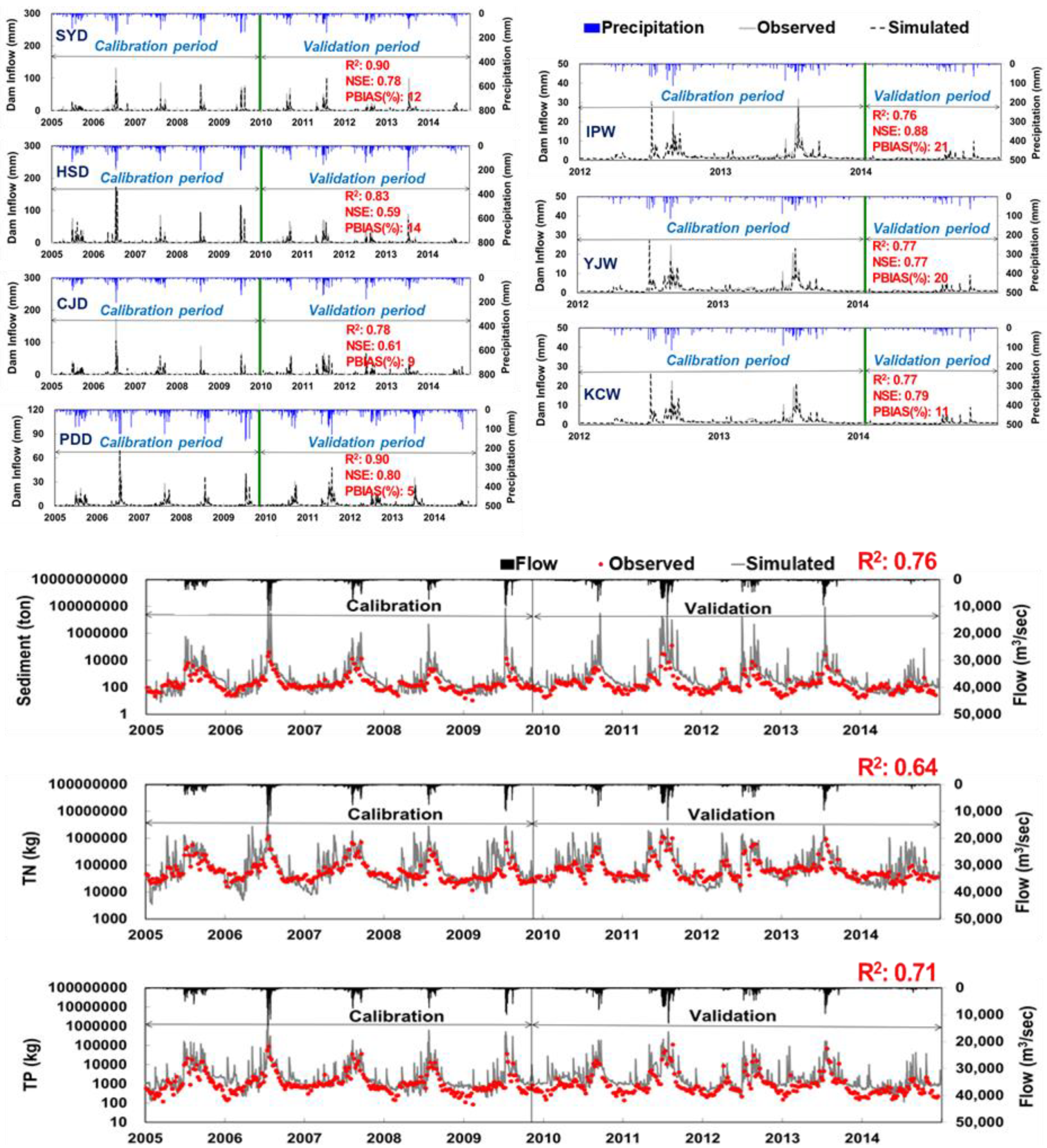
The SWAT streamflow at seven locations was calibrated and validated over 10 years (2005~2014) with R² (Determination coefficient) of 0.59 to 0.93, NSE (Nash and Sutcliffe model Efficiency) [37] from 0.57 to 0.95, and PBIAS from 4.5 to 21.4%. The suspended solid (SS), total nitrogen (T-N), and total phosphorus (T-P) of R² average values were 0.54, 0.42, and 0.47, respectively. These values satisfied the criteria specified in the SWAT calibration guidelines (NSE ≥ 0.5, PBIAS ≤ 28%, and R² ≥ 0.6) [38,39]. Figure 2a shows the calibrated and validated result of SWAT for daily dam inflow at seven locations and Figure 2b represents the results for eight days of data of SS, T-N, and T-P at one water quality station located nearby PDD where two main rivers are joined. More detailed information on the results for this study are presented in further papers (see [40,41,42,43]).

2.4. Random Forest Algorithm

Machine learning is the study of automated knowledge acquisition from multiple data sources [44] and classified into three learning methods: supervised learning, unsupervised learning, and reinforcement learning. Supervised learning includes algorithms such as Random Forest, Logistic Regression, Linear Discriminant Analysis, K-nearest Neighbors Classifier and Gaussian Naïve Bayes. Among them, Random Forest gives good results on many practical problems and has been used in environmental studies. Random Forest, proposed by Breiman [25], is an ensemble method that generates multiple bootstrap samples, applies the decision tree model to the samples, and then combines the results. One of the disadvantages of decision tree algorithms, the poor prediction performance caused by overfitting to train set, is supplemented by using bootstrap sampling that decreases the correlation between decision trees. A forest is formed by individual decision trees, which is created for each bootstrap sample. After, the Random Forest selects the class with the most votes for every tree in the forest. The performance of Random Forest depends on the strength of the individual trees and the correlation between the trees.

The classification trees in the Random Forest consist of nodes. Nodes are classified based on Gini index by selecting input variables that increase homogeneity within nodes and heterogeneity among nodes at every stage during tree growth from parent nodes to child nodes. The Gini index computes impurity in data using Equation (4).

$$\mathrm{Gini}\mathrm{index}=\sum _{i=1}^{r}P\left(i\right)\left(1-P\left(i\right)\right)$$

(4)

where r is the number of object variable categories and P(i) is the probability of being classified as i category. A small value of the Gini index indicates low heterogeneity within the node. A candidate value with minimum impurity (the smallest Gini index) is selected as a branch reference value for input variables in data partitioning [45].

In this study, the input variables of algorithm were water quality concentration and water temperature in spring (April to June) and fall (August to October). The AEH index (FAI, TDI, and BMI) grades were used as object variables. Among the 313 AEH monitoring sites, data of 86 sites were used considering the location of water quality observation stations, monitoring sites, and sub-watershed outlets. Although the performance can be improved by tuning the parameters with the number of trees and the variables selected in tree splitting, the default of parameters was adopted because it required less tuning than other algorithms, such as support vector machines [46,47].

3. Results and Discussion

3.1. The Stream Water Quality and Temperature Simulated by SWAT

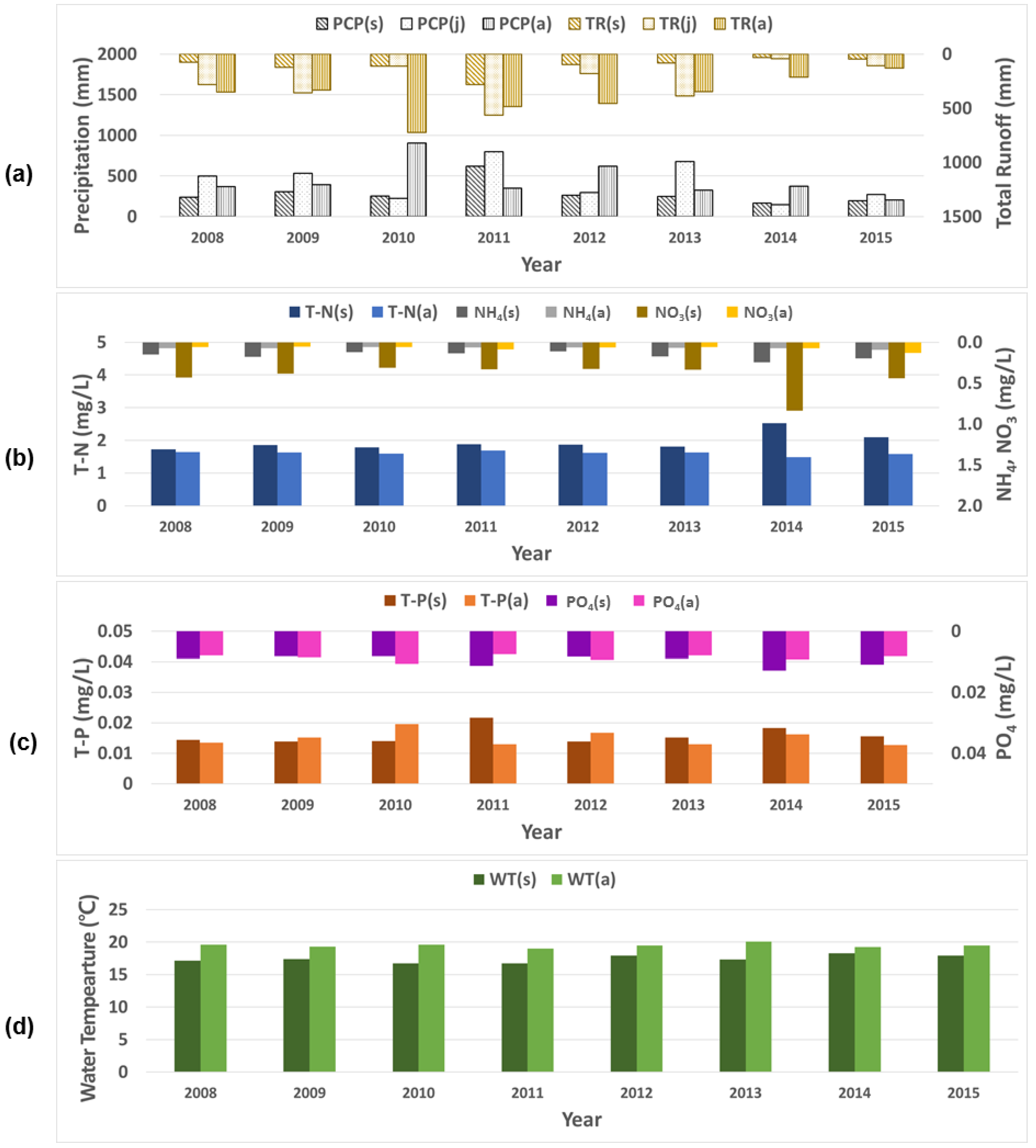
The SWAT simulated the stream water quality concentration (T-N, NH₄, NO₃, T-P, and PO₄) and water temperature (WT) of the 86 AEH sites to use them as input variables of Random Forest algorithm. Figure 3 shows the annual changes (2008~2015) of precipitation, total runoff, water quality concentration and water temperature considering seasonal variation for the whole watershed. The eight years average concentrations of T-N, NH₄, and NO₃ were 1.78, 0.12, and 0.25 mg/L respectively. Nitrogen-related water quality was higher in spring than fall, because the paddy rice irrigation in South Korea begins from middle of May with fertilizers. The T-N and NO₃ concentrations were the highest at 2.52 and 0.84 mg/L in spring 2014 (Figure 3b) due to decreased stream discharge affected by the severe drought (Figure 3a). The average concentrations of T-P and PO₄ were 0.015 and 0.0092 mg/L, respectively. The difference of T-P concentrations between spring and fall were bigger in 2010 and 2011 than the other six years (Figure 3c). As for the high T-P in fall 2010 and in the spring of 2011, this was due to the high rainfall compared with other years’ rainfalls and discharged to stream with particulate-dominant phosphorus attached to suspended solid from watershed runoff. The average water temperature was 17.43 °C in spring and 19.47 °C in fall with no significant difference (Figure 3d).

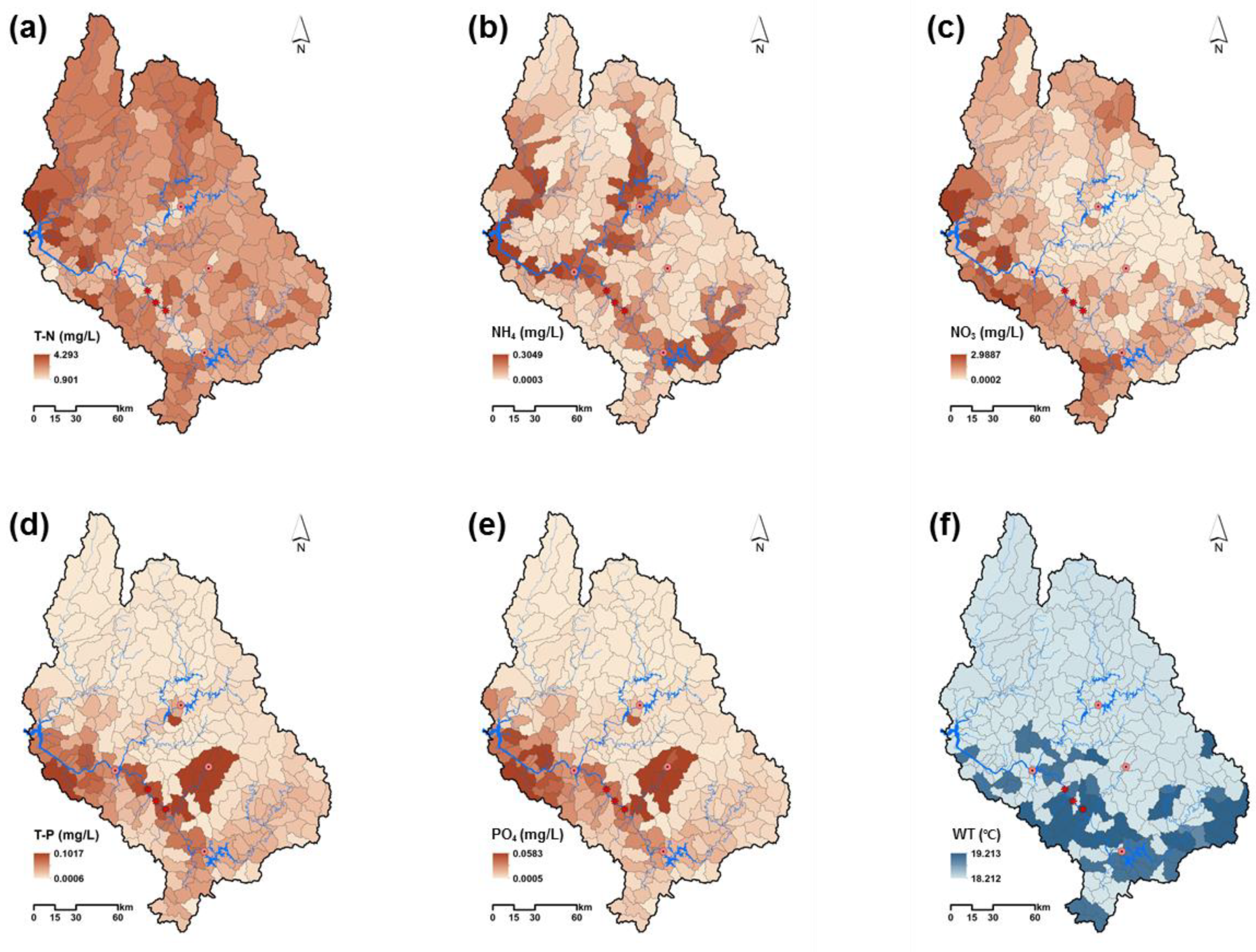
As seen in Figure 4 and Figure 1d, the NH₄ showed high concentrations in rice paddy areas along the stream. The NO₃ showed high concentration in the urbanized areas of downstream watershed and the highland agricultural areas of upstream watershed. From the NH₄ and NO₃, the T-N showed more or less high concentrations as it goes to the downstream of the watershed. The T-P and PO₄ concentrations were high in the urbanized areas by the sewage discharges and the agricultural areas along the downstream of the watershed. The water temperature was higher in the southern areas of the watershed (Figure 4).

3.2. Performance of Random Forest Classification Algorithm

The ratio for train data and test data was 7:3 in Random Forest application. For the training, the grade of AEH indices (FAI, TDI and BMI), water quality concentrations (T-N, T-P, NH₄, NO₃, and PO₄) and water temperature during the AEH observed period were applied. For the test, the AEH indices grade were verified from the water quality concentrations and water temperature for the Random Forest performance.

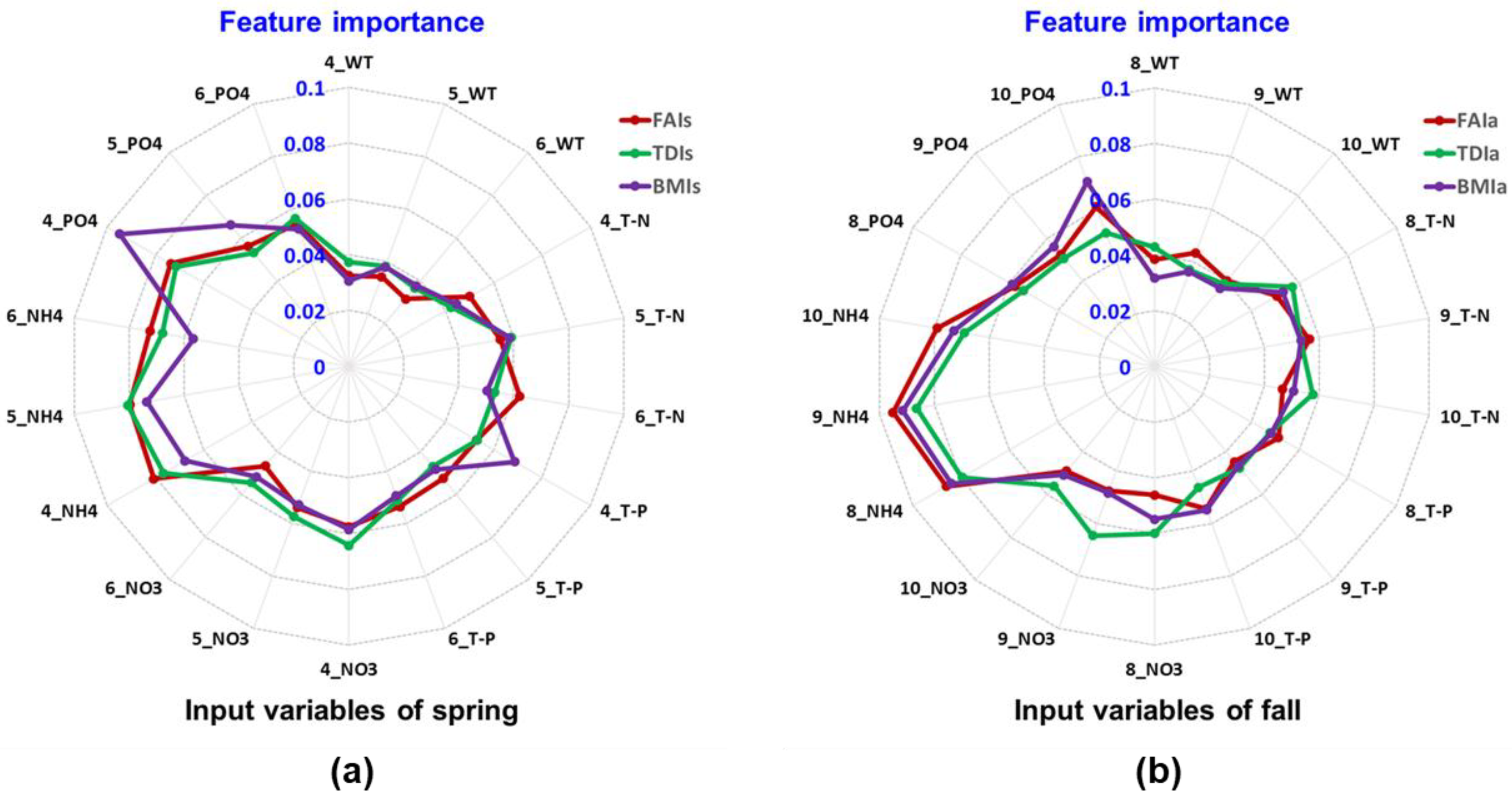
Feature importance is calculated as the decrease in node impurity due to splits in each variable. The variable with the higher feature importance is more important as it contributes more to the reduction of node impurity. Figure 5 shows the feature importance of input variables, where the prefix number represents month. During the observing periods, the NH₄ in spring and fall showed relatively higher importance than others. It meant that the NH₄ had more impact on FAI, TDI, and BMI classification. The T-P in April, and PO₄ in April and October were important with BMI. There was weak relationship with water temperature discussed by Woo [48].

Table 2. The classification result for each grade of three AEH indices for spring and fall seasons.

Grade		FAI				TDI				BMI
		P	R	F1	S	P	R	F1	S	P	R	F1	S
Spring	A	0.63	0.62	0.63	61	-	-	-	0	0.80	0.90	0.85	164
	B	0.35	0.50	0.41	50	0.48	0.39	0.43	41	0.35	0.31	0.33	45
	C	0.33	0.35	0.34	52	0.45	0.67	0.54	82	0.33	0.16	0.22	25
	D	0.33	0.10	0.15	30	0.44	0.34	0.38	83	0	0	0	20
	E	0.50	0.38	0.43	8	0.60	0.49	0.54	69	0.34	0.59	0.43	17
Avg		0.43	0.43	0.42	201	0.49	0.48	0.48	275	0.60	0.65	0.62	271
Fall	A	0.61	0.68	0.65	60	-	-	-	0	0.76	0.92	0.83	153
	B	0.43	0.53	0.47	55	0.20	0.04	0.07	25	0.41	0.34	0.37	64
	C	0.37	0.33	0.35	57	0.45	0.65	0.53	92	0.17	0.04	0.06	26
	D	0.36	0.20	0.26	25	0.59	0.17	0.22	80	0.10	0.06	0.07	17
	E	0	0	0	4	0.51	0.58	0.50	78	0.22	0.31	0.26	13
Avg		0.45	0.47	0.45	201	0.40	0.44	0.40	275	0.56	0.62	0.58	273

P = precision, R = recall, F1 = F1 score, and S = support (the number of each grade).

is the classification report for P, R, F1 score, and S of AEH index grades. The precision (P), known as the positive predictive value, is the ratio of the number of entries belong to a class among output data that are expected to belong to the class. The recall (R) is called the sensitivity. It is calculated as the ratio of the number of entries that are expected to belong to a class among the entries of the class. The F1 score is defined as the weighted harmonic mean of P and R, where the best F1 score is 1 and the worst value is 0. The support (S) is the number of instances in each class [49].

In spring, the average F1 score of FAI, TDI, and BMI was 0.42, 0.48, and 0.62 and in fall, it was 0.45, 0.40, and 0.58 respectively. The P, R, and F1 of BMI showed the highest values with the biggest S in both spring and fall. As the S was small, the P, R, and F1 value for the three AEH indices had tendency to decrease. Even the S was only eight for grade E in spring FAI, the P, R, and F1 showed high values of 0.50, 0.38, and 0.43 comparing with the grades B, C, and D in the condition of 50, 52, and 30 S. The reason is explained from the high relationship between water quality concentrations and AEH indices for grade E [48]. We can infer that the performance of P, R, and F1 for grades B, C, and D can be improved with S greater than 30, as seen in Table 2.

The confusion matrix is used to analyze and understand the misclassified grade analysis showing the number of each grade predicted by the random forest classifier and helps to compute the accuracy of overall and individual class label and to compare the predicted value and actual data set [50]. The matrix diagonal indicates the correspondence between the predicted value and actual ecological status, and it is used to calculate the accuracy of the algorithm [51]. The upper right part of the diagonal represents the number that is predicted to be lower than the real grade, and the lower left part shows the number that is predicted to be higher than actual value.

Table 3. The confusion matrix for each grade of three AEH indices.

Grade		FAI					TDI					BMI
		A	B	C	D	E	A	B	C	D	E	A	B	C	D	E
Spring	A	38	15	7	1	0	0	0	0	0	0	148	14	1	1	0
	B	11	25	13	1	0	0	16	20	2	3	24	14	4	0	3
	C	8	23	18	3	0	0	7	55	13	7	4	5	4	1	11
	D	3	8	13	3	3	0	3	39	28	13	7	5	3	0	5
	E	0	1	3	1	3	0	7	7	21	34	1	2	0	4	10
Fall	A	41	11	7	1	0	0	0	0	0	0	141	11	1	0	0
	B	15	29	11	0	0	0	1	18	4	2	29	22	4	4	5
	C	7	24	19	7	0	0	3	60	19	10	5	13	1	3	4
	D	4	4	12	5	0	0	1	33	14	32	6	5	0	1	5
	E	0	0	3	1	0	0	0	22	11	45	4	3	0	2	4

shows the confusion matrices for each classification result of Random Forest algorithm for test set. For spring FAI, TDI, and BMI, the sum of lower grade than actual data among misclassified value (upper right part from the diagonal) was 43, 58, and 40 and the sum of higher predicted classes (lower left part from the diagonal) was 71, 84, and 55 respectively. Most misclassified grades were assigned to one rank of grade difference except TDI fall grade E to C (value of 22) and BMI spring grade C to E (value of 11). It showed that the Random Forest classifier model tended to evaluate stream environment as being in better ecological status than the actual with the sum of upper right part from the diagonal (43, 58, 40) was smaller than the sum of lower left part (71, 84, 59). For fall FAI, TDI, and BMI, the sum of lower grade than actual data among misclassified value was 37, 85, and 37 and the sum of higher predicted classes among mislabeling value was 70, 70, and 67 respectively. Both the spring and fall TDI showed the worst predictions of 84 and 85 respectively. The trophic diatom may have other considerable factors such as physical characteristics of bed material and slope environment to represent the healthiness for TDI prediction in addition to the water quality and temperature components.

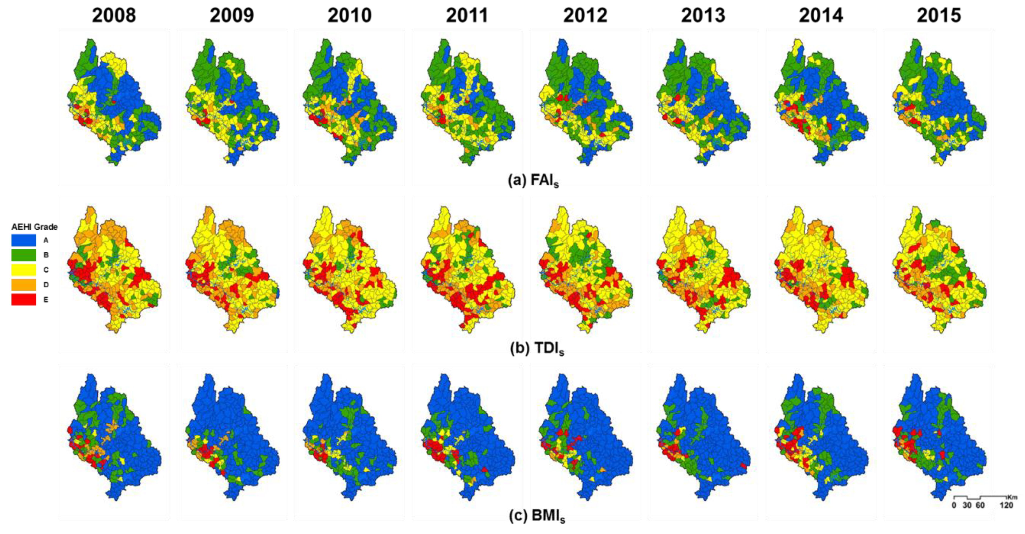
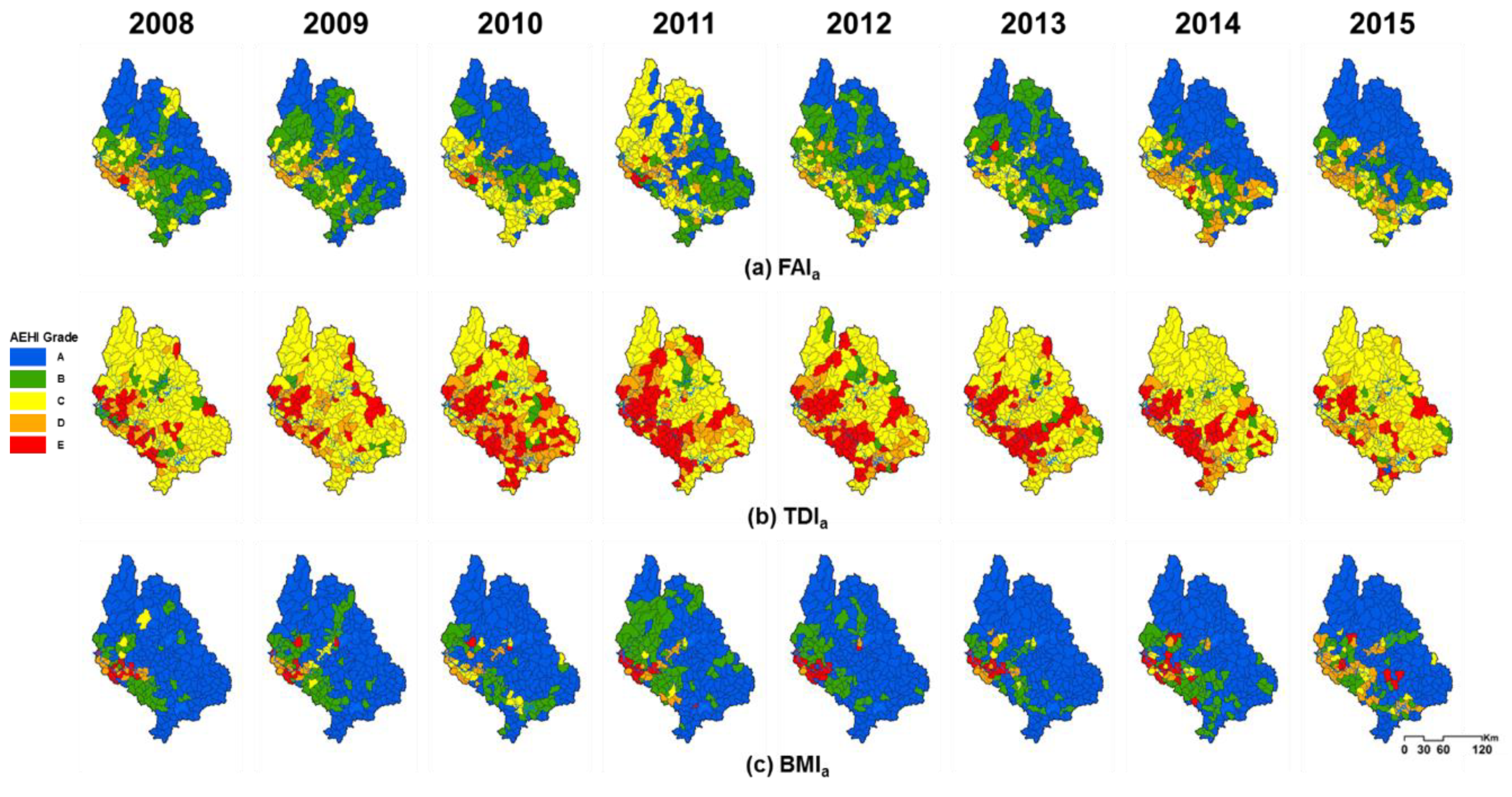
3.3. Evaluation of the AEH Index to the Whole Watershed Streams

The AEH of the whole watershed was assessed by applying the 86 sub-watersheds Random Forest trained algorithms to 237 sub-watersheds with SWAT results.

Table 4. Summary of the evaluated AEH for 237 sub-watersheds of Han river including the ungauged areas in spring (2008–2015).

Index	Grade	2008		2009		2010		2011		2012		2013		2014		2015
FAIs	A	88	(37%)	73	(31%)	73	(31%)	45	(19%)	73	(31%)	78	(33%)	86	(36%)	82	(35%)
	B	67	(28%)	81	(34%)	86	(36%)	93	(39%)	88	(37%)	87	(37%)	74	(31%)	83	(35%)
	C	62	(26%)	70	(30%)	49	(21%)	79	(33%)	56	(24%)	53	(22%)	45	(19%)	53	(22%)
	D	13	(6%)	8	(3%)	19	(8%)	14	(6%)	14	(6%)	14	(6%)	19	(8%)	14	(6%)
	E	7	(3%)	5	(2%)	10	(4%)	6	(3%)	6	(2%)	5	(2%)	13	(6%)	5	(2%)
TDIs	A	0	(0%)	1	(0%)	0	(0%)	0	(0%)	0	(0%)	0	(0%)	0	(0%)	0	(0%)
	B	31	(13%)	24	(10%)	18	(8%)	30	(13%)	42	(18%)	27	(13%)	21	(9%)	43	(18%)
	C	90	(38%)	109	(46%)	133	(56%)	97	(41%)	102	(43%)	119	(50%)	122	(52%)	120	(51%)
	D	71	(30%)	64	(27%)	41	(17%)	52	(22%)	54	(23%)	53	(22%)	60	(25%)	46	(19%)
	E	45	(19%)	39	(17%)	45	(19%)	58	(24%)	39	(16%)	38	(16%)	34	(14%)	28	(12%)
BMIs	A	143	(61%)	170	(72%)	161	(68%)	159	(67%)	166	(70%)	169	(72%)	137	(58%)	155	(65%)
	B	57	(24%)	35	(15%)	44	(19%)	37	(16%)	39	(16%)	43	(18%)	50	(21%)	50	(21%)
	C	5	(2%)	8	(3%)	15	(6%)	15	(6%)	11	(5%)	3	(1%)	22	(9%)	8	(3%)
	D	17	(7%)	10	(4%)	10	(4%)	4	(2%)	4	(2%)	5	(2%)	6	(3%)	6	(3%)
	E	15	(6%)	14	(6%)	7	(3%)	22	(9%)	17	(7%)	17	(7%)	22	(9%)	18	(8%)

and

Table 5. Summary of the evaluated AEH for 237 sub-watersheds of Han river including the ungauged area in fall (2008–2015).

Index	Grade	2008		2009		2010		2011		2012		2013		2014		2015
FAIa	Ν	96	(40%)	94	(40%)	91	(38%)	66	(28%)	80	(34%)	101	(42%)	110	(46%)	116	(49%)
	B	75	(32%)	85	(36%)	52	(22%)	58	(24%)	91	(38%)	87	(37%)	37	(16%)	39	(17%)
	C	36	(15%)	37	(15%)	71	(30%)	87	(37%)	49	(21%)	39	(16%)	40	(17%)	41	(17%)
	D	28	(12%)	21	(9%)	21	(9%)	22	(9%)	17	(7%)	9	(4%)	48	(20%)	41	(17%)
	E	2	(1%)	0	(0%)	2	(1%)	4	(2%)	0	(0%)	1	(1%)	2	(1%)	0	(0%)
TDIa	A	0	(0%)	0	(0%)	0	(0%)	0	(0%)	0	(0%)	0	(0%)	0	(0%)	2	(1%)
	B	19	(8%)	5	(2%)	6	(3%)	7	(3%)	10	(4%)	9	(4%)	7	(3%)	9	(4%)
	C	156	(66%)	158	(66%)	90	(38%)	108	(45%)	115	(49%)	143	(60%)	136	(57%)	160	(67%)
	D	24	(10%)	37	(16%)	55	(23%)	42	(18%)	34	(14%)	22	(9%)	33	(14%)	31	(13%)
	E	38	(16%)	37	(16%)	86	(36%)	80	(34%)	78	(33%)	63	(27%)	61	(26%)	35	(15%)
BMIa	A	175	(74%)	155	(65%)	164	(69%)	134	(57%)	173	(73%)	175	(74%)	146	(62%)	153	(65%)
	B	38	(16%)	57	(24%)	38	(16%)	74	(31%)	46	(20%)	35	(15%)	60	(25%)	32	(13%)
	C	3	(1%)	6	(3%)	18	(8%)	3	(1%)	0	(0%)	5	(2%)	6	(2%)	12	(5%)
	D	12	(5%)	12	(5%)	15	(6%)	12	(5%)	3	(1%)	10	(4%)	7	(3%)	34	(14%)
	E	9	(4%)	7	(3%)	2	(1%)	14	(6%)	15	(6%)	12	(5%)	18	(8%)	6	(3%)

show the number of sub-watersheds that evaluated each grade of three AEH indices, and Figure 6 and Figure 7 represent the annual AEH grade. The grade A of FAI and BMI are distributed at the upstream watershed. The TDI grade A does not exist in the watershed and the TDI grades from B to E were sensitive from year to year. This means that the TDI is sensitive to water quality especially NH4 concentration, which has the higher feature importance than others.

As seen in Table 4 and Table 5, the 2011 spring and fall AEH of three indices showed the negative movement from grade A to lower grades compared to other years. Looking at the figures, the bad grades were spread in space with FAI from grades A and B to C, TDI from grades C and D to E, and BMI from grade D to E in spring, and with FAI from grades A to B and C and BMI from grade A to B in fall respectively. As shown in Table 1, the 2011 spring rainfall and runoff are greater than other years, and this can be the main cause of grade degradation by the increase of pollutant discharges from agricultural areas along the stream and urbanized areas at the downstream watershed. For fall 2011, the large rainfall in July might affect the degradation of AEH of FAI and BMI.

4. Summary and Conclusions

In this study, Random Forest algorithm was used to evaluate the aquatic ecosystem health (AEH) of Han River in South Korea. The input variables of algorithm were SWAT stream water quality (T-N, T-P, NH₄, NO₃, and PO₄) concentration and water temperature and the objective variables are the grade of AEH indices (FAI, TDI, and BMI) in 86 stream locations.

The performance of Random Forest was represented as the classification reports and the confusion matrix. The classification results showed that the average accuracy (F1 score) of spring FAI_s, TDI_s, BMI_s, and fall FAI_a, TDI_a, and BMI_a for the input variables were 0.42, 0.48, 0.62, 0.45, 0.40, and 0.58, respectively. The number of data S (support) was lower than 30, and the accuracy showed poor F1 score. From the result of confusion matrix, the algorithm showed that the grade number of predicted classification was greater than that of actual classification. The TDI showed the worst prediction among the indices, which was inferred to consider another input variables such as the physical characteristics of bed material and slope environment because the trophic diatom is attached in the stream bed materials.

Using the trained and tested Random Forest, the AEH of 86 locations were extended to 237 ungauged locations covering the whole watershed by 237 sub-watersheds SWAT simulation. The result showed that the grade of downstream urbanized AEH was low by and large comparing with the grade of upstream mountainous AEH. Like the 86 locations result, the ecological health of fall was slightly recovered compared to spring by the streamflow increase and the water quality improvement by experiencing the rainy season of June to July.

From this study, it is recommended that measures are taken to recover the stream ecological status where the AEH index is below grade D, generally by agricultural activities in upstream areas and urban sewage discharges in downstream areas. for a target watershed This study can be used to make an aquatic ecosystem assessment of watershed streams that has limited field sites and monitoring data with the help of watershed water quality modeling and machine learning. Further research can be done by including a broad range of factors such as flow rate, stream water depth and width.

References

- Faber, M.; Rapport, D. Ecosystem Health: New Goals for Environmental Management, 1st ed.; Island Press: Washington, DC, USA, 1992; pp. 239–256. [Google Scholar]
- Vörösmarty, C.J.; McIntyre, P.B.; Gessner, M.O.; Dudgeon, D.; Prusevich, A.; Green, P.; Glidden, S.; Bunn, S.E.; Sullivan, C.A.; Liermann, C.R.; et al. Global threats to human water security and river biodiversity. Nature 2010, 467, 555–561. [Google Scholar] [CrossRef] [PubMed]
- Kelly, M.G.; Whitton, B.A. The trophic diatom index: A new index for monitoring eutrophication in rivers. J. Appl. Phycol. 1995, 7, 433–444. [Google Scholar] [CrossRef]
- Hering, D.; Johnson, R.K.; Kramm, S.; Schmutz, S.; Szoszkiewicz, K.; Verdonschot, P.F. Assessment of European streams with diatoms, macrophytes, macroinvertebrates and fish: A comparative metric-based analysis of organism response to stress. Freshw. Biol. 2006, 51, 1757–1785. [Google Scholar] [CrossRef]
- Johnson, R.K.; Furse, M.T.; Hering, D.; Sandin, L. Ecological relationships between stream communities and spatial scale: Implications for designing catchment-level monitoring programmes. Freshw. Biol. 2007, 52, 939–958. [Google Scholar] [CrossRef]
- Stoddard, J.L.; Herlihy, A.T.; Peck, D.V.; Hughes, R.M.; Whittier, T.R.; Tarquinio, E. A process for creating multimetric indices for large-scale aquatic surveys. J. N. Am. Benthol. Soc. 2008, 27, 878–891. [Google Scholar] [CrossRef]
- Mathuriau, C.; Silva, N.M.; Lyons, J.; Rivera, L.M.M. Fish and macroinvertebrates as freshwater ecosystem bioindicators in Mexico: Current state and perspectives. In Water Resources in Mexico; Springer: Berlin/Heidelberg, Germany, 2012; Volume 7, pp. 251–261. [Google Scholar] [CrossRef]
- Cheimonopoulou, M.T.; Bobori, D.C.; Theocharopoulos, I.; Lazaridou, M. Assessing ecological water quality with macroinvertebrates and fish: A case study from a small Mediterranean river. Environ. Manag. 2011, 47, 279–290. [Google Scholar] [CrossRef] [PubMed]
- Schultz, R.; Dibble, E. Effects of invasive macrophytes on freshwater fish and macroinvertebrate communities: The role of invasive plant traits. Hydrobiologia 2012, 684, 1–14. [Google Scholar] [CrossRef]
- Aazami, J.; Esmaili-Sari, A.; Abdoli, A.; Sohrabi, H.; Van den Brink, P.J. Monitoring and assessment of water health quality in the Tajan River, Iran using physicochemical, fish and macroinvertebrates indices. J. Environ. Health Sci. Eng. 2015, 13, 29. [Google Scholar] [CrossRef]
- Round, F.E. Diatoms in river water-monitoring studies. J. Appl. Phycol. 1991, 3, 129–145. [Google Scholar] [CrossRef]
- Leland, H.V. Distribution of phytobenthos in the Yakima River basin, Washington, in relation to geology, land use and other environmental factors. Can. J. Fish. Aquat. Sci. 1995, 52, 1108–1129. [Google Scholar] [CrossRef]
- Hill, B.H.; Stevenson, R.J.; Pan, Y.; Herlihy, A.T.; Kaufmann, P.R.; Johnson, C.B. Comparison of correlations between environmental characteristics and stream diatom assemblages characterized at genus and species levels. J. North Am. Benthol. Soc. 2001, 20, 299–310. [Google Scholar] [CrossRef] [Green Version]
- Lee, S.W.; Hwang, S.J.; Lee, J.K.; Jung, D.I.; Park, Y.J.; Kim, J.T. Overview and application of the national aquatic ecological monitoring program (NAEMP) in Korea. Ann. Limnol. Int. J. Limnol. 2011, 47, S3–S14. [Google Scholar] [CrossRef]
- KMA (Korea Meteorological Administration). Climate Change Status and Response Plan Report; KMA: Seoul, Korea, 2008; p. 2.
- Arnold, J.G.; Srinivasan, R.; Muttiah, R.S.; Williams, J.R. Large area hydrologic modeling and assessment part I: Model development 1. JAWRA J. Am. Water Resour. Assoc. 1998, 34, 73–89. [Google Scholar] [CrossRef]
- Kim, J.G.; Park, Y.; Yoo, D.; Kim, N.W.; Engel, B.A.; Kim, S.J.; Kim, K.S.; Lim, K.J. Development of a SWAT Patch for Better Estimation of Sediment Yield in Steep Sloping Watersheds 1. JAWRA J. Am. Water Resour. Assoc. 2009, 45, 963–972. [Google Scholar] [CrossRef]
- Lee, M.; Park, G.; Park, M.; Park, J.; Lee, J.; Kim, S. Evaluation of non-point source pollution reduction by applying Best Management Practices using a SWAT model and QuickBird high resolution satellite imagery. J. Environ. Sci. 2010, 22, 826–833. [Google Scholar] [CrossRef]
- Ahn, S.R.; Jeong, J.H.; Kim, S.J. Assessing drought threats to agricultural water supplies under climate change by combining the SWAT and MODSIM models for the Geum River basin, Korea. Hydrol. Sci. J. 2016, 61, 2740–2753. [Google Scholar] [CrossRef]
- Townsend, C.R.; Hildrew, A.G.; Francis, J. Community structure in some southern English streams: The influence of physicochemical factors. Freshw. Biol. 1983, 13, 521–544. [Google Scholar] [CrossRef]
- Winterbourn, M.J.; Collier, K.J. Distribution of benthic invertebrates in acid, brown water streams in the South Island of New Zealand. Hydrobiologia 1987, 153, 277–286. [Google Scholar] [CrossRef]
- Blinn, D.W. Diatom community structure along physicochemical gradients in saline lakes. Ecology 1993, 74, 1246–1263. [Google Scholar] [CrossRef]
- Dodds, W.K.; Jones, J.R.; Welch, E.B. Suggested classification of stream trophic state: Distributions of temperate stream types by chlorophyll, total nitrogen, and phosphorus. Water Res. 1998, 32, 1455–1462. [Google Scholar] [CrossRef]
- Shahnawaz, A.; Venkateshwarlu, M.; Somashekar, D.S.; Santosh, K. Fish diversity with relation to water quality of Bhadra River of Western Ghats (India). Environ. Monit. Assess. 2010, 161, 83–91. [Google Scholar] [CrossRef] [PubMed]
- Breiman, L. Random forests. Mach. Learn. 2001, 45, 5–32. [Google Scholar] [CrossRef]
- Gislason, P.O.; Benediktsson, J.A.; Sveinsson, J.R. Random forests for land cover classification. Pattern Recognit. Lett. 2006, 27, 294–300. [Google Scholar] [CrossRef]
- Prasad, A.M.; Iverson, L.R.; Liaw, A. Newer classification and regression tree techniques: Bagging and random forests for ecological prediction. Ecosystems 2006, 9, 181–199. [Google Scholar] [CrossRef]
- Chan, J.C.W.; Paelinckx, D. Evaluation of Random Forest and Adaboost tree-based ensemble classification and spectral band selection for ecotope mapping using airborne hyperspectral imagery. Remote Sens. Environ. 2008, 112, 2999–3011. [Google Scholar] [CrossRef]
- Grossmann, E.; Ohmann, J.; Kagan, J.; May, H.; Gregory, M. Mapping ecological systems with a random forest model: Tradeoffs between errors and bias. Gap Anal. Bull. 2010, 17, 16–22. [Google Scholar]
- Vincenzi, S.; Zucchetta, M.; Franzoi, P.; Pellizzato, M.; Pranovi, F.; De Leo, G.A.; Torricelli, P. Application of a Random Forest algorithm to predict spatial distribution of the potential yield of Ruditapes philippinarum in the Venice lagoon, Italy. Ecol. Model. 2011, 222, 1471–1478. [Google Scholar] [CrossRef]
- Granata, F. Evapotranspiration evaluation models based on machine learning algorithms—A comparative study. Agric. Water Manag. 2019, 217, 303–315. [Google Scholar] [CrossRef]
- Kamińska, J.A. A random forest partition model for predicting NO2 concentrations from traffic flow and meteorological conditions. Sci. Total Environ. 2019, 651, 475–483. [Google Scholar] [CrossRef]
- Silveira, E.M.; Silva, S.H.G.; Acerbi-Junior, F.W.; Carvalho, M.C.; Carvalho, L.M.T.; Scolforo, J.R.S.; Wulder, M.A. Object-based random forest modelling of aboveground forest biomass outperforms a pixel-based approach in a heterogeneous and mountain tropical environment. Int. J. Appl. Earth Obs. Geoinf. 2019, 78, 175–188. [Google Scholar] [CrossRef]
- Ministry of Environment. Nationwide Aquatic Ecological Monitoring Program; National Institute of Environmental Research: Incheon, Korea, 2015.
- Arnold, J.G.; Williams, J.R.; Srinivasan, R.; King, K.W. SWAT Manual; USDA. Agricultural Research Service and Black land Research Center: Temple, TX, USA, 1996.
- Neitsch, S.L.; Arnold, J.G.; Kiniry, J.R.; Williams, J.R. Soil and Water Assessment Tool Theoretical Documentation Version 2009; Texas Water Resources Institute: Temple, TX, USA, 2011. [Google Scholar]
- Nash, J.E.; Sutcliffe, J.V. River flow forecasting through conceptual models part I—A discussion of principles. J. Hydrol. 1970, 10, 282–290. [Google Scholar] [CrossRef]
- Moriasi, D.N.; Arnold, J.G.; Van Liew, M.W.; Bingner, R.L.; Harmel, R.D.; Veith, T.L. Model evaluation guidelines for systematic quantification of accuracy in watershed simulations. Trans. ASABE 2007, 50, 885–900. [Google Scholar] [CrossRef]
- Santhi, C.; Arnold, J.G.; Williams, J.R.; Dugas, W.A.; Srinivasan, R.; Hauck, L.M. Validation of the swat model on a large river basin with point and nonpoint sources 1. JAWRA J. Am. Water Resour. Assoc. 2001, 37, 1169–1188. [Google Scholar] [CrossRef]
- Ahn, S.R.; Kim, S.J. Assessment of Climate Change Impacts on the Future Hydrologic Cycle of the Han River Basin in Korea Using a Grid-Based Distributed Model. Irrig. Drain. 2016, 65, 11–21. [Google Scholar] [CrossRef]
- Ahn, S.R.; Kim, S.J. Assessment of integrated watershed health based on the natural environment, hydrology, water quality, and aquatic ecology. Hydrol. Earth Syst. Sci. 2017, 21, 5583–5602. [Google Scholar] [CrossRef] [Green Version]
- Ahn, S.R.; Lee, J.W.; Jang, S.S.; Kim, S.J. Large Scale SWAT Watershed Modeling Considering Multi-Purpose Dams and Multi-Function Weirs Operation-For Namhan River Basin. J. Korean Soc. Agric. Eng. 2016, 58, 21–35. (In Korean) [Google Scholar] [CrossRef]
- Ahn, S.R. Physically-Based Watershed Health and Resilience Assessment Considering Climate Change. Ph.D. Thesis, Graduate School of Konkuk University, Seoul, Korea, 2016. [Google Scholar]
- Langley, P.; Simon, H.A. Applications of machine learning and rule induction. Commun. ACM 1995, 38, 54–64. [Google Scholar] [CrossRef]
- Pal, M. Random forest classifier for remote sensing classification. Int. J. Remote Sens. 2005, 26, 217–222. [Google Scholar] [CrossRef]
- Fernández-Delgado, M.; Cernadas, E.; Barro, S.; Amorim, D. Do we need hundreds of classifiers to solve real world classification problems? J. Mach. Learn. Res. 2014, 15, 3133–3181. [Google Scholar]
- Probst, P.; Bischl, B.; Boulesteix, A.L. Tunability: Importance of hyperparameters of machine learning algorithms. arXiv 2018, arXiv:1802.09596. [Google Scholar]
- Woo, S.Y.; Jung, C.G.; Kim, J.U.; Kim, S.J. Assessment of climate change impact on aquatic ecology health indices in Han river basin using SWAT and random forest. J. Korea Water Resour. Assoc. 2018, 51, 863–874. (In Korean) [Google Scholar] [CrossRef]
- Goutte, C.; Gaussier, E. A probabilistic interpretation of precision, recall and F-score, with implication for evaluation. In Proceedings of the European Conference on Information Retrieval, Santiago de Compostela, Spain, 21–23 March 2005; Springer: Berlin/Heidelberg, Germany, 2005; pp. 345–359. [Google Scholar] [CrossRef]
- Benediktsson, J.A.; Swain, P.H.; Ersoy, O.K. Neural network approaches versus statistical methods in classification of multisource remote sensing data. IEEE Trans. Geosci. Remote Sens. 1990, 28, 540–552. [Google Scholar] [CrossRef]
- Congalton, R.G. A review of assessing the accuracy of classifications of remotely sensed data. Remote Sens. Environ. 1991, 37, 35–46. [Google Scholar] [CrossRef]
Figure 1.
Description of study area: (a) Major hydraulic structure (Dam and Weir), Observation stations (Weather, Evapotranspiration, Soil Moisture, Groundwater level, Water quality, and aquatic ecosystem health (AEH)), (b) Digital Elevation Model (DEM), (c) Soil type, and (d) Land use.
Figure 2.
The calibration and validation results of SWAT for (a) dam inflow and (b) water quality [40,41,42,43].
Figure 3.
The comparison of the SWAT seasonal average results; (a) Precipitation and total runoff, (b) Water quality component related to Nitrogen (T-N, NH4, NO3), (c) Water quality component related to Phosphorus (T-P and PO4), and (d) Water temperature from 2008 to 2015, the characters in the bracket (s), (j), and (a) represent spring, July, and fall respectively.
Figure 4.
The spatially averaged distribution during 2008~2015: (a) Total Nitrogen (T-N), (b) Ammonium (NH4), (c) Nitrate (NO3), (d) Total Phosphorus (T-P), (e) Phosphate Phosphorus (PO4), and (f) Water Temperature (WT).
Figure 5.
The feature importance of Random Forest input variables T-N, NH4, NO3, T-P, and PO4 and WT (a) spring and (b) fall.
Figure 6.
AEH of Han river evaluated by (a) FAIs, (b) TDIs, and (c) BMIs in spring (2008–2015).
Figure 7.
AEH of Han river evaluated by (a) FAIa, (b) TDIa, and (c) BMIa in fall (2008–2015).