An Approach to Determining the Spatially Contiguous Zone of a Self-Organized Urban Agglomeration

1
Institute of Mountain Hazards and Environment, Chinese Academy of Sciences, Chengdu 610041, China
2
Branch of Mountain Sciences, Kathmandu Center for Research and Education, Chinese Academy of Sciences, Chengdu 610041, China
3
School of Resources, Sichuan Agricultural University, Chengdu 611130, China
*
Authors to whom correspondence should be addressed.
Sustainability 2019, 11(12), 3490; https://0-doi-org.brum.beds.ac.uk/10.3390/su11123490
Submission received: 17 May 2019
/
Revised: 14 June 2019
/
Accepted: 15 June 2019
/
Published: 25 June 2019
(This article belongs to the Section Sustainable Urban and Rural Development)
Abstract
:The evolution of the urban agglomeration is a significant development in urban geography. Determining its spatial range for effective measurement remains a challenge for researchers. In previous studies, determining spatial range has primarily been done through distinguishing the cities that should belong to urban agglomerations from among other cities by using various indicators. Both the selection of indicators and the standards used for calculation and identification have been based on subjective choices, and have not considered spatial distribution or morphology. The urban agglomeration can be regarded as a self-organized space, and spatial features of the fractal can be regarded as one of the morphological characterizations of spatial self-organization. From the perspective of the assumption that the space of urban agglomerations is molecule like assembled, and through the extraction and analysis of spatial fractals, we present an objective method to determine the “spatially contiguous zone” of urban agglomeration, particularly the spatial range in which the urban agglomeration is able to exercise jurisdiction within the radius of its capacity, rather than in the administrative division. Our method is applied in this paper to the Beijing–Tianjin–Hebei urban agglomeration and produced the following results: (1) the existence of spatial fractals and the theory of space unit molecule like self-organization or assembly in the morphology of urban agglomerations has been proved; and (2) a spatially contiguous zone could be identified for the urban agglomeration has been confirmed. Compared with previous methods used for determining space, this method is centered on the spatial morphology of urban agglomerations; the recognition of a spatially contiguous zone liberates the geographical limits of the result from city boundary restrictions. Concurrently, by considering the linkages within the city as a self-organizing black box, we can circumvent the one-sidedness involved with the selection of indicators that has biased previous studies, thereby avoiding having to focus on the specific mechanism of urban dynamics, and coming much closer to its self-organizing dynamic inner nature. This approach will prove to be a useful reference for the identification of spatial ranges in future studies.
Keywords:
urban agglomeration; spatially contiguous zone; space range identification; self-organization; fractalTerms:
spatially contiguous zone; molecule like assembly; assembly radius1. Introduction
Urban agglomeration is the result of urban spatio-temporal evolution. The effective measurements used to determine these clusters are the foundation for studies on the spatio-temporal evolution of urban agglomerations, thus helping to optimize land-use policies and implement spatial controls. Identifying the spatial range of an urban agglomeration effectively depends on the basic measurement of the urban agglomeration. The spatial range of an urban agglomeration must be defined effectively for analysis of the evolution and management of urban agglomerations to be implemented. Therefore, determining the explicit spatial range of an urban agglomeration is the premise and the basis for conducting relevant research. However, the complexity and openness of urban agglomerations make the spatial range fuzzy and thus hard to demarcate [1]. Defining the urban agglomeration and identifying its spatial range remains a major issue in urban geography.
There is still no uniform definition of urban agglomeration in academia. Since the concept was first put forward, “town cluster”, “megalopolis”, “urban agglomeration”, and other similar concepts have successively emerged. Ebenezer Howard contributed the origin of town clusters from the perspective of garden city [2], and suggested that the area around the city should be included in the urban planning scope. Gottmann defined the urbanized area connected by several cities or metropolitan areas as megalopolises [3], and Yao, Gu, and Fang consider the aggregation that consist of multiple cities with central city is urban agglomerations [1,4,5]. Thus, different scholars have presented different understandings of the urban agglomeration. There are also some scholars treated the polycentricity as the representation of urban agglomeration [6,7], and explored the essence of urban agglomeration from the agglomeration of factors [8].
Establishing spatial range has been a subject of many studies, which were mostly aimed at identifying the boundary of an individual city. Studies to identify spatial range in relation to urban agglomerations are lacking. Methods for identifying spatial range in existing studies can be roughly divided into three approaches. The first approach takes the administrative boundary as the spatial range of the urban agglomeration, which makes the designated range larger than the actual range [9] and renders it impossible to aggregate the urban areas near the boundaries in relation to neighboring urban agglomerations [10,11]. The second approach sets criteria for selecting individual cities as members of an urban agglomeration. Scholars have used different criteria to define the membership of different urban agglomerations [1,12,13]. Index analysis is a mature method in the field of spatial identification, but it completely or partially ignores the spatial information regarding the urban agglomeration and the possibility of an urban agglomeration having aggregated parts of the space in individual cities. Moreover, this method cannot avoid subjective bias in the selection of the indicators used. The third approach is to judge whether a nearby city can be included in the urban agglomeration by using models to analyze the connection between cities based on the selection of central cities. Since Martin proposed a method of calculation to determine the boundary of a metropolitan area [14], scholars have attempted to establish different models to further study this issue, such as the gravity model, the breakpoint model, the field-strength model, and the Voronoi model [9,15,16,17]. These model-based methods take urban spatial distribution and the interactions between urban areas into account, which is closer to the actual situation than in the first two approaches. However, it is still the case that the indicators used for calculating the models and the selection of judging criteria cannot avoid subjective bias, and the method for measuring the flow of elements in the development process lacks scientifically robust evidence, rendering universal acceptance difficult to achieve. From a general perspective, previous research to identify the space of an urban agglomeration has taken individual cities as the identified unit. Such research studies have ascertained the spatial range of an urban agglomeration purely by distinguishing whether an individual city belongs to a particular urban agglomeration. The result is a city aggregation where space range is defined by a specific and precise city’s boundary, which ignores the fact that only part of the city may be classified into an urban agglomeration as well as the actual spatial morphology of urban aggregation. Beyond this, most methods of analysis involve a discrimination process based on calculations of indicators, in which the selection of the indicator and the establishment of criteria are both highly subjective and optional. In these methods, the indicators which are spatially contiguous cannot actually be counted, which makes it hard to describe the urban agglomeration objectively.
Spatial fractal features are considered to be a language to describe nature and can be used as one of the tools to represent the spatial morphology of geographic objects. Extracting and analyzing spatial fractal features allows the measurement of spatial objects based on morphology. In terms of the studies on fractal cities, perhaps the most major contributors are Batty and Longley. Michael Batty, who is a member of the British Academy of Sciences, has been researching fractals and cities since the 1970s, and put forward the original concept of fractal cities in 1991. Batty published the book Fractal Cities: A Geometry of Form and Function in collaboration with Longley in 1994. This work discussed the fractal features of the boundary, the land form, and the urban growth of cities. In 1995, Batty published the paper Fractals: New Ways of Looking at Cities in the journal Nature, and pointed out that fractals are effective tools for looking at cities. Recent scholarship has attempted to delimit the range for a single city by analyzing the spatial fractal features of urban morphology from the perspective of morphology. Rozenfeld et al. put forward the City Cluster Algorithm [18,19]. It is not fractal-based, but it provides a logical basis for analyzing the spatial fractal geometry. Tannier et al. tried to identify the boundary of Basel agglomeration (regions forming an individual urban area rather than the agglomeration composed of collective cities) by using a polynomial fit method to find the most deviated point, based on the fractal geometry of Basel urban area [20]. However, a polynomial fit has no clear mathematical structure and lacks robust plausibility for making effective inferences about the system. Tannier et al. applied the same method to define urban territories by identifying functional agglomerations (regions forming an individual functional area rather than an agglomeration composed of collective cities) in order to extract and characterize the morphological boundaries of both theoretical and real urban units by using fractal and non-fractal indices [21]. Tan et al. integrated neighborhood dilation theory into Tannier’s work, and used a multi-period curve to identify urban boundaries based on raster data [22]. Chen used a q-order scaling exponent spectra of multifractal structures to characterize urban-rural terrain quantitatively [23]. Previously, Openshaw had developed a geographic analysis machine and researched clustering by using a shifting search-circle based on the spatial distribution of points [24,25]. Although these works did not target the urban agglomeration, they provided the groundwork for spatial range identification from the standpoint of spatial morphology.
The original description of a contiguous zone, as defined by the United Nations Convention on the Law of the Sea [26], is a band of water extending from the outer edge of a territorial sea, within which a state can exert limited control. To address the limitations of the previous research on urban agglomeration spatial range outlined above, our research learns from the thought of a contiguous zone over which jurisdiction could be exercised. This approach does not require treating the individual city as the identified unit of the spatial range of an urban agglomeration. Therefore, we break the geographical limits of a city’s boundary set, and name the built parcels as well as the continuous and associated regions among them within an urban agglomeration as the spatially contiguous zone. Thus, we recognize the spatial range as the object in which the urban agglomeration has the ability to exercise jurisdiction including influences derived from spatial interaction, flow of elements in development processes, energy flows, material flows, movement of population, and the other processes. Next, we introduced Tannier’s method, which was used for identifying the boundaries of urban areas (the individual urban areas composed of regions), to measure the fractality of the urban agglomeration (the agglomeration composed of collective cities), and undertook research to present here an objective method to recognize a spatially contiguous zone for urban agglomerations, viewing space units assemblies from the perspective of self-organization in urban agglomerations. This method treats the flat, continuous, and associated region as the primary focus and visualizes the region of the recognized spatial range as one in which the urban agglomeration has the capacity to exercise jurisdiction without being separated by specific city boundaries. This approach brings us closer to a spatial range in which the urban agglomeration does indeed exercise jurisdiction. At the same time, we regard the urban agglomeration as a self-organizing black box and recognize the spatial range in which the urban agglomeration can exercise jurisdiction objectively through the fractal, without selecting indicators to statistically determine urban units. This will avoid the one-sidedness and arbitrary nature of the selection of indicators that has beset past research and help to approach the inner dynamics of self-organization. Finally, we apply this approach to the Beijing–Tianjin–Hebei urban agglomeration, recognizing the spatially contiguous zone, and verifying the validity of this method.
2. The Theory of Molecular Assembly in Urban Agglomeration Spaces
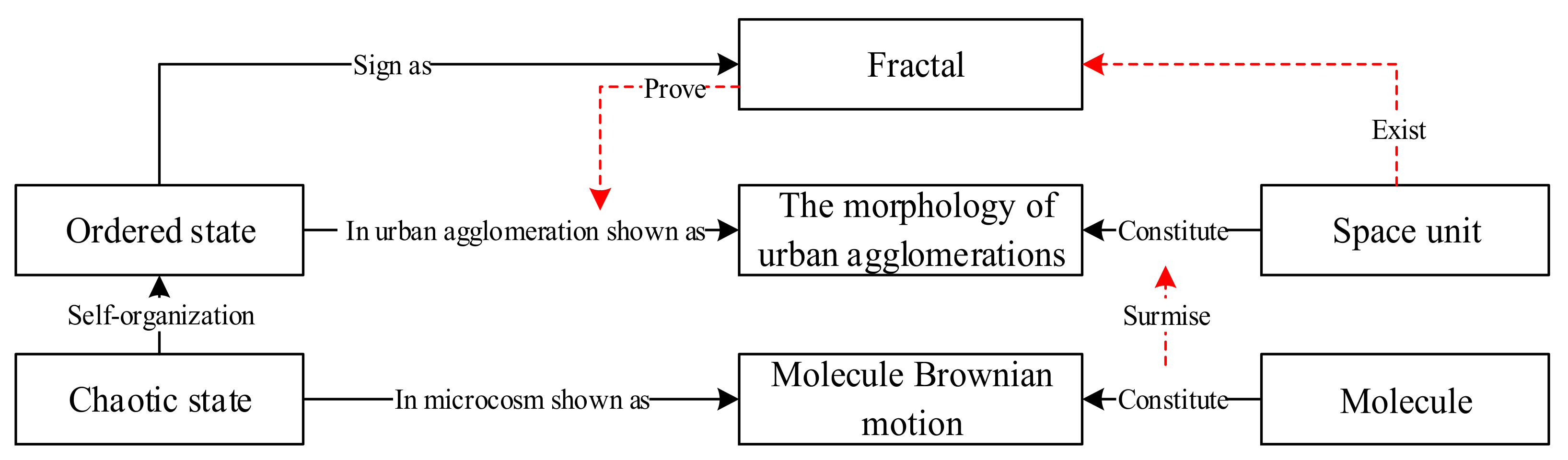
The self-organizing evolution of urban areas, which are complex systems, has been confirmed by much research [27,28,29,30,31,32,33]. Self-organization is a process in which chaos is transformed into an ordered state. The state of chaos is demonstrated in a microcosm by molecules in Brownian motion. The substance composed of molecules comes to maintain an orderly and stable state eventually through molecular interactions, and the fractal is the by-product of this process. It can be said that the fractal is one symbol of self-organizing characteristics, and that spatial fractality comes from the evolution of spatial self-organization [28,34]. If the scale of a phenomenon changes in a regular way and can be measured at a dimension corresponding to this regularity, then this phenomenon can be called fractal [30]. The process of determining the point of regularity is the measurement of fractals. Fractals require two essential conditions: regular changes that can be recorded with a scale of measurement and self-similarity [30]. The former is often a result of the latter, and is assessed with a metric known as the fractal dimension.
This paper adopts the viewpoint of Yao that urban agglomerations can be regarded as clusters that have swallowed multiple towns [1], an urban agglomeration can be interpreted as clusters assembled by space units. Diverse factors, including the natural environment, the social environment, the economic environment, and the supply and demand dynamics, conspire to give urban agglomerations their chaotic and nonlinear characteristics. We regard the urban agglomeration as a black box in which these factors are self-organizing, and assume that the town (or smaller space units) in urban agglomerations are the equivalent of molecules on a non-representational level acting in a self-organizing state, which are the elementary particles in microcosms. Hence, if we can prove the existence of a fractal as a characteristic of space units’ distribution in terms of space, which is the outcome of the self-organizing process, then we can confirm that the space of urban agglomerations is characterized by an inner assembly process. In this situation, the space of urban agglomerations can be considered to be being constituted by such town-like non-representational elementary particles. It may also include parts of a town, such as a block, a parcel, etc. Thus, we referred to all these non-representational elementary particles by the term space units, generally. The derivation procedures for the theory of molecule like assembly of urban agglomerations can be observed in Figure 1.
3. The Method to Measure the Spatial Fractality of Urban Agglomerations from the Perspective of Space Unit Spatial Assembly
There are several ways of measuring spatial fractality as shown by the existing research. Fractals are commonly identified by changes in the measurement scale. Using different metrics with different degree scales to measure the same spatial morphology, we can obtain different results. If r is the degree scale and the corresponding number is N(r), we could get a series of corresponding counts while the degree scales of the rulers continuously change. If the two variables for degree scale and number meet the following relationship (Equation (1)):
where this is the case we can confirm that the spatial morphoogy involves scaling invariance and self-similarity, which meet the necessary characteristics of fractals, where D is the fractal dimension.
If we regard urban agglomerations as being formed by clusters of towns or other smaller space units, they should exhibit both continuity and discreteness in their spatial distribution. Urban agglomeration is considered a complete entity by the scale, but it can also be considered to be being composed of independent individual units. Therefore, this study unifies the changing measurement scales and changes in composition, and measures the spatial fractality of urban agglomerations’ spatial morphology, using a method for measuring fractality from the perspective of space unit assembly.
Based on the perspective of space unit assembly, we regard the discrete towns or smaller space units in urban agglomerations as the equivalent of the molecules acting in a self-organizing state in microcosms. When the distance between two space units is less than a critical degree, the non-representational attraction between them will suddenly increase, and they will aggregate in a non-representational sense. We can visualize that space units have assembled non-representationally and that space unit clusters have appeared. This procedure is termed space unit spatial assembly in our study, and the “critical distance” involved is the assembly radius. Additionally, all the space units involved in the assembly constitute the spatial volume of the urban agglomeration, and the combination of the units determines its spatial morphology, which is assembled by space units. The internal logic of the non-representational changes in space is shown in Figure 2:
To measure the spatial fractality of urban agglomerations from the perspective of space unit spatial assemblies, we must regard the critical distances of the non-representational aggregations occurring between the space units, the assembly radii, as different degree scales on different rulers. When the distance is changed, the quantity and spatial distribution of the assembled space units also changes. We then obtain different sets of assembled space units, which represent the volume of urban agglomerations, by changing the assembly radius; the space unit clusters consisting of different sets of assembled space units present different spatial morphologies, as shown in Figure 3. Thus, the number of space unit clusters obtained from different spatial morphologies is the total, which is obtained by measuring the spatial fractality with different rulers.
The main idea underlying the measurement of spatial fractality in this paper can be summarized as follows: Based on the space units (such as spatial patches) in the study area, we set up an isometric shifty series with different assembly radii r. Fusing the space units between which the respective distances are less than the assembly radii, we get the assembled space unit clusters. To measure the number (or area) of clusters, we get a set of different counts N(r) corresponding to different degree scales r, if they meet the following relationship (Equation (2)):
Thus, it can be considered that the urban agglomeration spatial morphology has the necessary characteristics of fractals, where D is the fractal dimension.
4. An Approach to Recognizing the Spatially Contiguous Zone of Urban Agglomerations Based on Based on Spatial Fractality
The spatially contiguous zone of an urban agglomeration as defined in this paper can be embodied as a contiguous polygon constituted by the minimum enveloped spatial region for each space unit cluster. According to the idea of space unit spatial assembly, the set of space units that have been assembled varies when the assembly radius changes, as does the volume of urban agglomeration and the number of space unit clusters. If we can confirm the existence of spatial fractality, then the relationship between the assembly radius r and the number of space unit clusters N(r) should be an effective power function. The power function relationship can then be equated with a double logarithmic linear relationship, such that:
Therefore, we can draw out the double logarithmic curve with the logarithm of the assembly radius r and the logarithm of the space unit clusters count N(r) using the data from the measurement of spatial fractality. If the fractality exists, the double logarithmic curve should express a linear variation. If there is only a limited range in which the fractality is expressed (i.e., scaling invariance) on real curves, this range can be called the non-scaling interval, and we can determine the existing range of spatial fractality by identifying the non-scaling interval. Thus, if the precondition that fractality is a characteristic of urban agglomerations’ spatial morphology can be confirmed, we can identify the spatial range of urban agglomeration by using the existing geographical range of spatial fractality.
In line with the aims of this study, to identify the non-scaling interval involves obtaining a segment of the double logarithmic curve with a linear or approximately linear shape. In a mathematical sense, and in theory, we can accurately identify the linear portion of the curve by the gradient of change in the curve. However, since the curve is generally obtained by fitting, and the spatial data have errors, a sample point lies only approximately on the curve. The gradient of each point on the linear portion fluctuates around a certain value. The curve cannot, in fact, represent the linear shape perfectly and the linear portion cannot be identified clearly.
Nevertheless, the horizontal portion of the gradient-changing curve can be identified through the second derivatives of the curve function. In addition, the curve function could be obtained through polynomial fitting. This process is similar to the one employed by a past study [20] that tried to find the most deviated point on the curve through the curvature function of the polynomial estimated curve, which is chosen by the Bayesian information criterion. However, a polynomial fit has no clear mathematical structure. Therefore, polynomial equations are always employed to make interpolation for a dataset rather than providing a description of the variation for a system. It is known in the theory of mathematical modeling that it is not always possible to make an effective inference through the multinomial model.
In this study, we identify the linear portion of the double logarithmic curve by the triangle derived from the samples. On the scatter diagram of the double logarithmic points, a triangle can be formed by the two endpoints and the inflexion point of the double logarithmic curve. If we regard the line between the two endpoints as the bottom side of the triangle, the inflexion point would be the point with the maximum distance from the bottom side in the double logarithmic curve [35]. The inflexion point would be the limit of the linear portion of the double logarithmic curve.
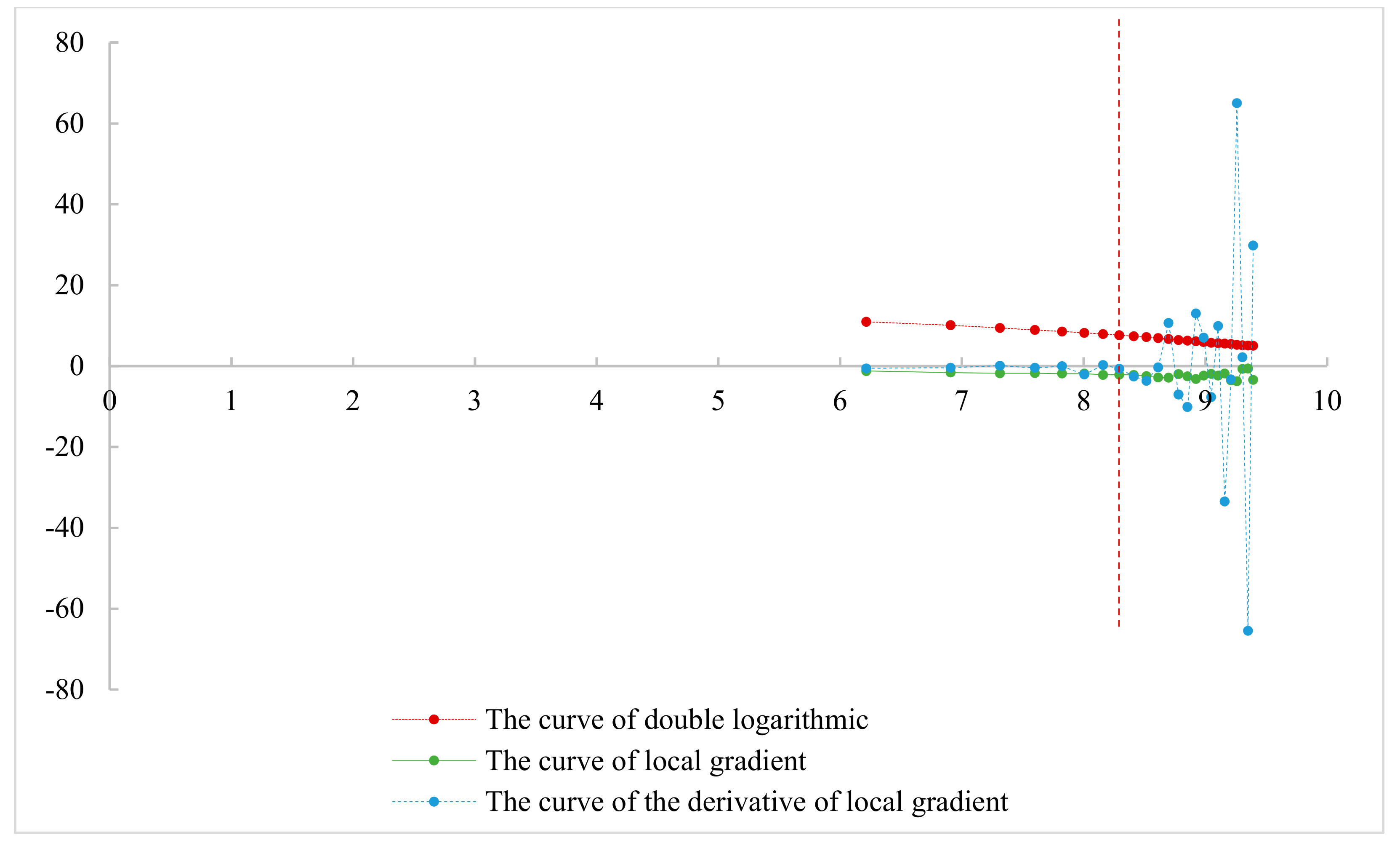
At the same time, to avoid errors derived from the identification of the inflexion point, we introduce the curve’s local gradient, and its derivative as the testing and verification tool (Table 1). By determining the local gradient and its derivative [36], based on sample points, we can plot the local gradient curve and its derivative double logarithmic curve.
Finally, by mapping the range of the spatial fractality onto the assembly radius of space units, we can recognize the set of assembled space units of an urban agglomeration. Furthermore, we can recognize the spatially contiguous zone of an urban agglomeration by the largest cluster of assembled space units at the assembly radius.
The whole process of recognizing the spatially contiguous zone of urban agglomerations based on spatial fractality is shown in Figure 4:
5. A Method to Validate the Effectiveness of the Recognized Spatially Contiguous Zone of Urban Agglomeration
To validate the representativeness of the space in which the urban agglomeration can exercise jurisdiction through a spatially contiguous zone, we introduce the coefficient of variation (Cv) as an indicator for measuring the features of the three groups of space unit samples: the units inside the zone, the units outside the zone, and the entire group of units. The coefficient of variation can be used for describing the degree of relative difference between different samples in one group. If we use the areas of the space units as samples to calculate the coefficient of variation, the coefficient is the ratio of the standard deviation (s) and the mean of the areas () of all space units:
The coefficient of variation can be used to evaluate the degree of relative differentiation between different samples in one group, and is, of course, the inherent feature of the group.
When a small group of samples is the subset of another larger group of samples, and if their coefficient of variation is the same or differs only marginally, then the small group is considered to be representative of the larger group. In other words, the small group could replace the large group to represent the inherent features of the large one. The representativeness of a spatially contiguous zone of an urban agglomeration can be validated by comparing the differentiated features of the three sample groups: the space units inside the spatially contiguous zone, the space units outside the spatially contiguous zone, and the space units in the whole space of urban agglomeration. If the representativeness of the spatially contiguous zone can be verified, then the spatially contiguous zone can be considered to be the spatial range in which the urban agglomeration has the ability to exercise jurisdiction.
6. The Beijing–Tianjin–Hebei Urban Agglomeration
The feasibility of this approach can be illustrated by applying it to a case study.
6.1. Data Source
For this case study, we have selected the Beijing–Tianjin–Hebei urban agglomeration based on the status of built-up land in 2016. The data are remote sensing images from the United States Landsat series land resources satellite. The study area encompasses the administrative districts of Beijing, Tianjin, and Hebei. The spatial extent of the study area is about 220,000km2. We extracted a vector polygon of land from remote sensing images divisionally by selecting 7,153 training samples, and classified them into four categories: developed land, agricultural land, mountains, and water. Then, by completing the mosaics of the vector polygons of developed land in the study area, which were extracted from the Landsat images, the vector data of currently developed land in the study area, totaling 129,883 patches, were obtained. Based on a visual comparison of remote sensing images and classification results, we deemed there to be high classification accuracy, which could recognize the spatial fractality of the study area.
6.2. Measuring the Spatial Fractality of the Urban Agglomeration
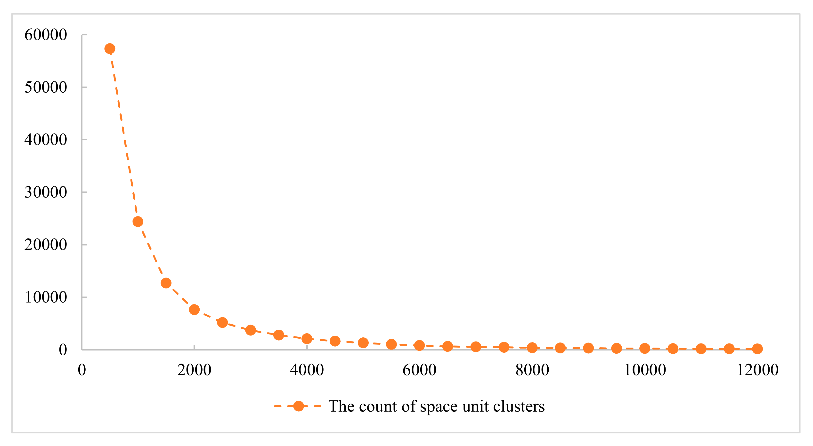
Based on our theory of space unit spatial assembly, this application regarded each vector polygon of the developed land as a space unit, and measured the space units (i.e., parcels) of the Beijing–Tianjin–Hebei urban agglomeration using the above-mentioned method (in Section 3). We employed an assembly radii series from 0.5km to 12km with equal space (0.5km) as rulers, and the number of space unit clusters as the measured cluster count. The applied assembly radius and the corresponding count of clusters in the Beijing–Tianjin–Hebei urban agglomeration in 2016 were measured by the above-mentioned method.
By plotting the assembly radius and its corresponding count of space unit clusters on a coordinate graph (Figure 5), we can conclude that the number of space unit clusters declined as the assembly radius increased, while the area of space unit clusters increased. From the measurements, we can see that the measurement data of different scales (i.e., assembly radius) involves scaling invariance that changes with the power law. Thus, the space units of the urban agglomeration demonstrate typical characteristics of the fractal from the perspective of space unit spatial assembly, thus satisfying Equation (2). We can confirm the existence of the fractality, which is the characteristic of urban agglomeration spatial morphology, and that our assumption holds.
Based on this information, to recognize the spatially contiguous zone, we had to determine the existing range of spatial fractality to obtain the corresponding assembly radius. Since the assembly radii and their corresponding count of clusters demonstrated typical fractality, which is the precondition to identify the spatial range of urban agglomerations, their logarithm should have exhibited this linear relation. Therefore, the linear non-scaling interval of the double logarithmic curve of the assembly radius and its corresponding count of space unit clusters should show the existing range of spatial fractality.
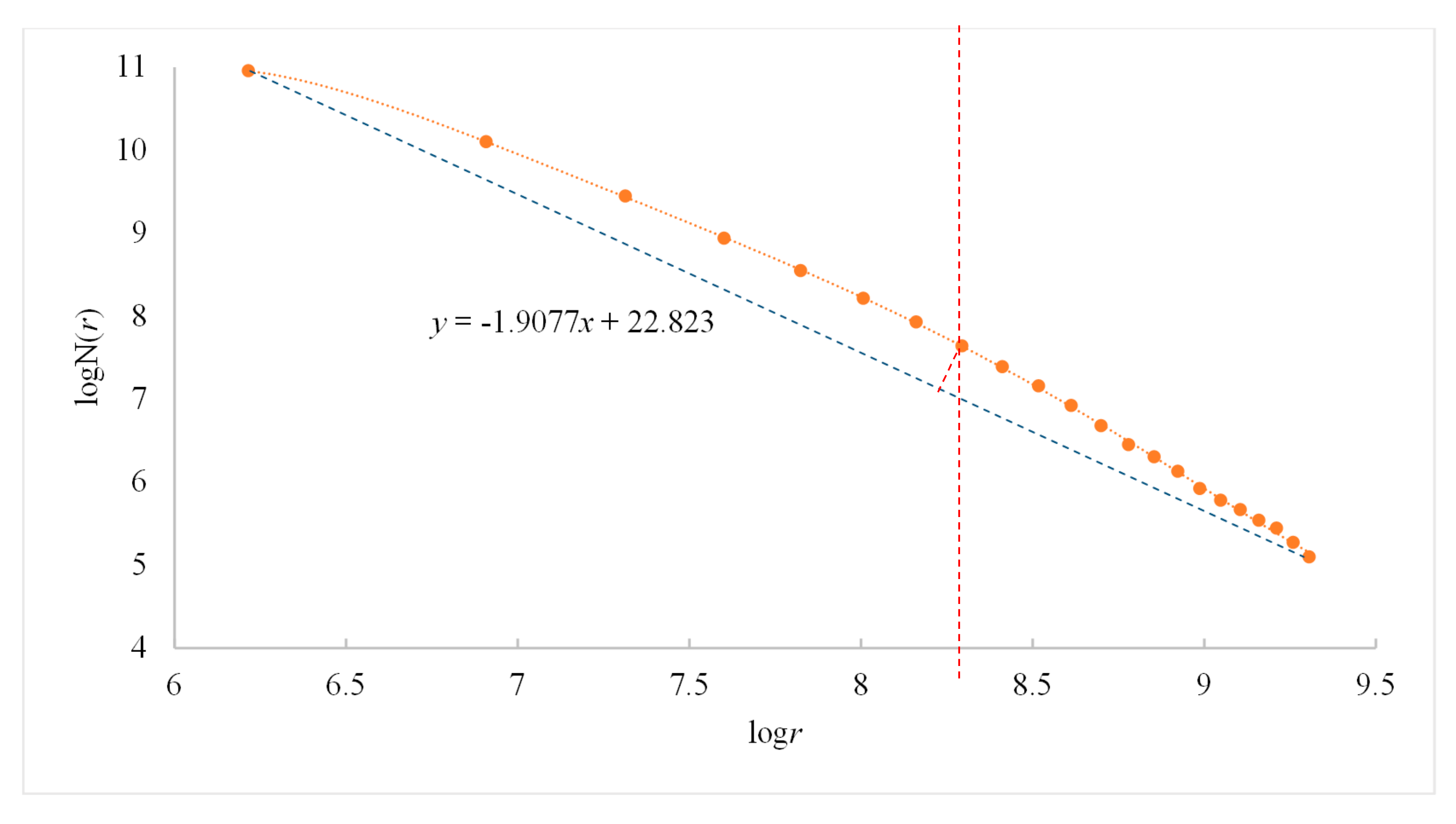
Based on the method to identify the non-scaling interval mentioned above, we had to recognize the inflexion point on the double logarithmic curve. As such, in this application, we plotted the double logarithmic points on the scatter diagram (Figure 6) and obtained the line between the two endpoints of the double logarithmic curve, which is the bottom side of a triangle. We calculated the distance from each sample point to the line by using the distance between point and line formula to find out the maximum distance and its corresponding sample point, which is the inflexion point on the double logarithmic curve. Our calculations are shown in Figure 6:
At the same time, to avoid the errors that come from the recognition of the inflexion point on the double logarithmic curve, we considered the pairs from the double logarithm of assembly radius and number of clusters as the sample points. By solving equations for the local gradient and its derivative based on the sample points, we plotted the local gradient curve and its derivative double logarithmic curve, as shown in (Figure 7). This was done to verify the reliability of the recognition of the inflexion point detailed above.
We can see from the figure above that there was only a limited range (i.e., non-scaling interval) for the linear double logarithmic curve of assembly radius and its corresponding count of clusters in the urban agglomeration exhibited the linear relation only approximately.
6.3. Recognizing the Spatially Contiguous Zone of the Urban Agglomeration
Based on the calculation of the distances between each sample point in the double logarithmic points and the bottom side of the triangle, the inflexion point would be the point when the logarithm of assembly radius is 8.29. The local gradient curve and its derivative curve (obtained when the logarithm of the assembly radius was less than 8.29) only fluctuated slightly within a limited range. Although it was not a strict linear relation, the fluctuation amplitude was small. From the local gradient derivative, it can be inferred that the absolute value of the rate of gradient change in this limited range falls within a range so small as to be virtually negligible relative to the total change. Therefore, it is possible to conclude that the double logarithmic curve exhibited the linear relation approximately. Conversely, when the logarithm was more than this value, the change of local gradient derivative was dramatic, and the local gradient exhibited variation from the original constant. The double logarithmic curve of the assembly radius and the number of space unit clusters exhibited a tendency to deviate from the approximate linear relation rather than the exact linear relation that should be exhibited from spatial fractality. For these reasons, we determined that the point with the logarithm of assembly radius of 8.29 was the existing threshold of spatial fractality.
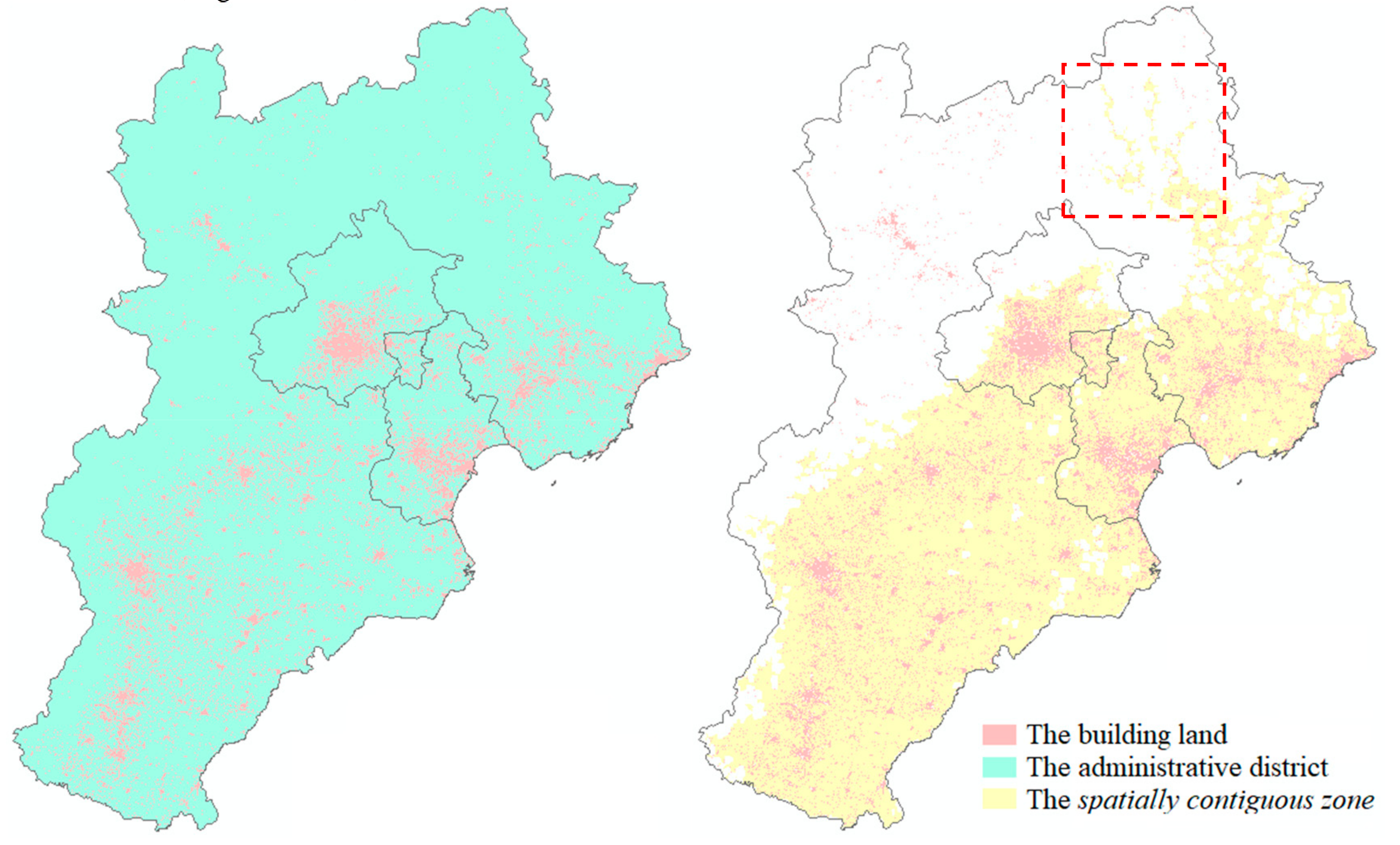
Finally, based on the logarithm of assembly radius at 8.29, we could infer that the assembly radius recognized as the existing threshold of spatial fractality was 4.0km. Based on this radius and the vector polygons of developed land in the study area, we fused the space units between which the spatial distance was less than the identified assembly radius; this gave us the assembled space unit clusters, which form the recognized spatially contiguous zone of the Beijing–Tianjin–Hebei urban agglomeration (Figure 8b).
6.4. Effectiveness Analysis
Based on these results, to validate the representativeness of the space over which the urban agglomeration has the capacity to exercise jurisdiction through its spatial contiguity, we calculated the coefficient of variation of the three sample groups: the space units inside the spatially contiguous zone, the space units outside the spatially contiguous zone, and the space units in the whole urban agglomeration space. The coefficient of variation of each group is shown in Table 2.
In Figure 8, we can see that the spatially contiguous zone (in Figure 8b) that we have identified differs from the conventional spatial range (in Figure 8a) composed of the urban administrative district for the urban agglomeration, which only covers parts of the conventional spatial range. Our model broke the restriction on keeping the integrity of the administrative district, better reflecting the independent and organic character of urban agglomerations, which differs from a set of multiple cities. The spatially contiguous zone of the urban agglomeration includes not only the existing built-up areas but also the non-urban areas between towns. This continuous distribution embodies the assemblage effect that occurred among the space units, and conforms to the characteristics of interaction that exist among the towns. Meanwhile, the spatially contiguous zone not only includes the whole region of the existing built-up area, but also reveals holes inside the spatially contiguous zone, which reflects the limitations of the interactions among the towns. The dendrite morphology in the northeast (outlined by a red box in Figure 8b) reflects the effect of natural obstacles on the interactions among the towns, and illustrates that the direction of spatial interaction is not in absolute straight lines. At the same time, the branch channel is also a reflection of the flow of elements in the development process. On the other hand, the patches of developed land in the spatially contiguous zone we have recognized appear to be obvious hierarchical structures in the spatial distribution, and the morphology conform with the "positive hexagon" hypothesis of Central Place Theory [37], suggesting that the spatially contiguous zone of the urban agglomeration is theoretically a scientifically rigorous conception. Overall, the results of our case study also coincide with the conventional wisdom on the major components of the Beijing–Tianjin–Hebei urban agglomeration.
Regarding the coefficient of variation, we can observe that the coefficient of variation of the space units inside the spatially contiguous zone was significantly higher than those outside, and that their difference from the entire administrative district was small. This demonstrates that the characteristics of the whole space of the urban agglomeration are primarily reflected in the space units inside the spatially contiguous zone; and the space units outside it had only a small effect on the characteristics of the whole urban agglomeration. This is in accordance with the first law of geography. Ultimately, this verified the effectiveness of representing the space of the urban agglomeration through recognizing the spatially contiguous zone.
In terms of the methods that we used, we can observe that the spatially contiguous zone of the urban agglomeration that we recognized is delimited based on the valid natural morphology of urban agglomerations. Only the morphological units that can illustrate the inherent spatial features (i.e., the fractality) can be recognized as the component unit of urban agglomeration (i.e., the assembled space units), while any morphological unit that cannot represent these features will be eliminated. The existing spatial features in an urban agglomeration are shaped according to various behaviors in the urban agglomeration, and these behaviors are determined by the specific functions themselves, which are considered the objective inevitability of the exertion of jurisdiction. Therefore, by using the collected evidence to make logical inferences it can be proved that using the spatially contiguous zone of an urban agglomeration to represent the spatial range in which the urban agglomeration has the capacity to exercise jurisdiction is objectively reasonable.
Applying these to the Beijing–Tianjin–Hebei urban agglomeration allowed us to verify the theory of space unit spatial assembly in urban agglomerations, and proved the feasibility and effectiveness of this approach in recognizing the spatially contiguous zone of an urban agglomeration.
7. Discussion
Compared with the traditional spatial range of urban agglomeration, our proposed spatially contiguous zone of urban agglomeration is a spatial range that the incorporated urban agglomeration has the capacity to touch and over which it can exercise jurisdiction as a single subject, reflecting the holistic character of the urban agglomeration rather than simply presenting a set of multiple cities. The continuity between towns can be reasonably claimed as an urban agglomeration’s exercise of jurisdiction over its survival space, and conforms to the characteristics of interaction that exist among the towns, while the irregular shape of the spatially contiguous zone also embodies a reasonable restriction of jurisdiction and interaction. Thus, the spatially contiguous zone is a reasonable recognition of the space in which the urban agglomeration has the capacity to exercise jurisdiction, without being separated by cities. Meanwhile, the towns in the spatially contiguous zone exhibit the hierarchical structures of spatial distribution that conform to the hypothesis of Central Place Theory, and can be regarded as an illustration of classical geographical theory.
Compared with traditional methods for identifying the spatial range of urban agglomerations (Table 3), the approach to recognizing a spatially contiguous zone of urban agglomerations proposed in this study has the following characteristics:
First, the spatially contiguous zone of an urban agglomeration is recognized from a macro perspective rather than an evaluation based on each city, thus breaking the spatial limits derived from the unit of identification. This approach allows us to identify that part of the space of the city vested in the urban agglomeration, realize the objective measurement of the spatial range of the urban agglomeration, and avoid the effect of the inseparability of the unit of identification on the final results.
Second, the identification method used in this research is based on the spatial morphology determined by the self-organization of urban agglomerations. It collects and analyzes the spatial information adequately, and regards the interactions and flows of elements in the development process of towns as the behavior of self-organization in a black box of urban agglomeration that does not require special consideration. It can recognize the urban agglomeration spatial range without having to identify influencing factors for the spatial structure and distribution of the urban agglomeration; and it avoids the negative effect arising from the imperfection of the methods used to identify factors on the final results.
Third, the approach used in this research could avoided measuring the centrality of the city. The direction of spatial interaction inside the urban agglomeration will not be limited to the linearity conventions established by traditional methods, for the recognized space of an urban agglomeration is omnidirectional. It can avoid the neglect of non-urban spatial direction, which results from only giving consideration to the interaction with central city, as well as the effects on identification results that come from the subjective bias on the selection of indicators and judging criteria used for determining the central city.
Fourth, the approach used in this research has avoided issues with indicator selection, and has added no subjective factors for consideration. This method for measuring spatial fractal features is an objective statistical method. The identification of the existing range of spatial fractality is essentially a calculation of fracture points without requiring any indicators, since mapping the non-scaling interval in space is defining a standard by objective means. Our approach to identifying an urban agglomeration can avoid the effects of subjective behavior in favor of an objective method for determining an urban agglomeration.
Finally, many studies have confirmed that the morphology of the urban area exists with multifractal characteristics [38,39,40,41,42,43,44,45], which reflect the different expressions of urban and non-urban areas. In contrast to what might appear to be the case, there are parts of non-urban area space that in fact belong to urban agglomerations. The identification method employed in this study can avoid a recognition of the multifractal with the level of scale, which could directly remove the non-urban agglomeration areas from the whole region without differentiating the urban agglomeration from the non-urban areas.
Compared with the similar research undertook by Tannier et al. [20], the method used in this research based on the mathematical property of the inflexion point. It has avoided the fitting of the multinomial model, which were always employed to make interpolation for a dataset without clear mathematical structure. Therefore, it is not necessary to searching a description for the variation curve. Unfortunately, since the study areas do not have the same scale, the criteria used for cartographic generalization are not the same, the spatial concepts, structure, extent, volume, living habits, population density, density of construction, level of development, etc. are different, there is no comparability among the values of the results obtained from these researches.
However, there seems to be a precondition to apply the approach just as the case in this paper that the double logarithmic curve of the assembly radius and the counts of clusters is expected to be linear at its beginning, which may be the majority of cases. If the gradient is stable in the middle of the double logarithmic curve but not at its beginning, it is still feasible to identify the maximum end of the non-scaling interval by recognizing inflexions. Since the interval before the non-scaling interval probably derived from the possibility that space units with tiny intervals would assembled at a smaller scale or they would not assembled since the inevitable repulsive force, or the finite data at beginning of the curve are limited by the measurement scale, and clusters assembled by a small radius can be flooded by clusters assembled by a maximum radius, it could be inferred that the maximum end of the non-scaling interval as the assembly radius. Furthermore, if there are several non-scaling intervals on the same double logarithmic curve, it is necessary to identify the maximum end of each gradient-stable intervals severally since different non-scaling intervals are corresponding to different spatially contiguous zones, which can be considered to be the serial of urban agglomeration’ space ranges corresponding to a serial of spatial scales and be used in different analysis scenarios. Therefore, the approach in this research can be applied in most cases.
8. Conclusions
An urban agglomeration is an aggregation formed by clusters of towns, built on the spatial interaction that exists between towns. Compared with the traditional gravity models, the urban agglomeration in this study has been regarded as a self-organizing black box, and using the perspective of molecule like assembly to understand and recognize the development of urban agglomerations essentially. Based on the spatial range in which the self-organization effect still occurs obtained by the measurement of fractality, recognition of a spatially contiguous zone representing the urban agglomeration is achievable. It discards the rigid spatial range which is based on the administrative boundaries of cities, avoids the selection of indicators, and circumvents any need to focus on the implicit mechanism of the evolution. Finally, based on a case study, the feasibility and effectiveness of our approach in recognizing a spatially contiguous zone has been verified and shown to provide helpful investigative procedures for identifying the spatial range of urban agglomerations.
The approach outlined in this paper can be applied to urban agglomerations’ formulation of development planning and policies, such as controlling the expropriation of built-up land, setting the development boundaries of urban agglomerations, determining the key monitoring areas and boundaries for ecological protection, searching for the unsuitable space earmarked for administrative action and others.
There is still much controversy concerning the concept and the identification of urban agglomerations [46,47,48,49]. In this study, we recognized a spatially contiguous zone, but our research does not imply that it is a method of measurement that can be used constantly. Different measurements will produce different results, and the method in this study should also be perfected further to accommodate different concepts concerning urban agglomerations, as the perspective of space unit spatial assembly would not be adapted if the urban agglomeration was not seen as a cluster.
Furthermore, the sample points cannot reflect the precise shape of the curve strictly. Because of the finite density of the assembly radii we employed as the degree scale, it is not possible for us to specify the identified assembly radius on meter-level (in this case was kilometer-level), which would influence the precision and the visual recognition of the non-scaling interval but could be improved by increasing the density of the assembly radius series we set up. Moreover, the study area under the larger scale might cause the loss of the precision since the coarser criterion used for cartographic generalization. Therefore, further research is required on how to improve the precision of the identified assembly radius unconditionally.
In addition, a future line of research will look to move the current single-time case study to a full spatio-temporal analysis looking at urban agglomeration evolution.
Author Contributions
Conceptualization, methodology, data analysis, F.L.; writing—original draft preparation, F.L.; writing—review and editing, Q.H.
Funding
This research was funded by the Special Institute Youth Training Program of IMHE (Grant No. SDS-QN-1911), the Science and Technology Service Network Initiative (Grant No. KFJ-STS-QYZD-060), the Strategic Priority Research Program of Chinese Academy of Sciences (Grant No. XDA19030303-02) and the Fund for Scientific Research in the Public Interest, Ministry of Land and Resources, China (Grant No. 201511010-07).
Acknowledgments
We would like to thank Nianjue Wang and Xinqi Zheng for their review and supervision. We would also like to thank Editage.com for providing help with the language.
Conflicts of Interest
The authors declare no conflict of interest. The funders had no role in the design of the study; in the collection, analyses, or interpretation of data; or in the writing of the manuscript.
References
- Yao, S.M.; Chen, Z.G.; Zhu, Y.M.; Guan, C.M.; Chen, S.; Guan, W.H.; Hu, G.; Li, C.F. The Urban Agglomeration of China; Press of University of Science and Technology of China: Hefei, China, 2006. [Google Scholar]
- Howard, E. Tomorrow: A Peaceful Path to Real Reform; Routledge: Abingdon, UK, 1994; Volume 6, p. 139. [Google Scholar]
- Gottmann, J. Megalopolis or the urbanization of the northeastern seaboard. Econ. Geogr. 1957, 33, 189–200. [Google Scholar] [CrossRef]
- Gu, C.L.; Chai, Y.W.; Cai, J.M.; Niu, Y.F.; Sun, Y.; Chen, T.; Ye, J.A. The Urban Geography of China; The Commercial Press: Beijing, China, 2002. [Google Scholar]
- Fang, C.L.; Song, J.T.; Zhang, Q.; Li, M. The Formation, Development and Spatial Heterogeneity Patterns for the Structures System of Urban Agglomeration in China. Acta Geogr. Sin. 2005, 60, 827–840. [Google Scholar]
- Halbert, L. The Polycentric City Region That Never Was: The Paris Agglomeration, Bassin Parisien and Spatial Planning Strategies in France. Built Environ. 2006, 32, 184–193. [Google Scholar] [CrossRef] [Green Version]
- Yang, T.R.; Pan, H.Z.; Hewings, G.; Jin, Y. Understanding urban sub-centers with heterogeneity in agglomeration economies—Where do emerging commercial establishments locate? Cities 2019, 86, 25–36. [Google Scholar] [CrossRef]
- Audretsch, B. Agglomeration and the location of innovative activity. Oxf. Rev. Econ. Policy 1998, 14, 18–29. [Google Scholar] [CrossRef]
- Chen, Q.Y.; Song, Y.X. Methods of dividing the boundary of urban agglomerations: Chang-Zhu-Tan Urban Agglomeration as a case. Sci. Geogr. Sin. 2010, 30, 660–666. [Google Scholar]
- Pan, J.H.; Liu, W.S. Identification of spatial influence sphere of urban agglomerations in China based on urban hinterland delimitation. Adv. Earth Sci. 2014, 29, 352–360. [Google Scholar]
- Wang, C.L.; Liu, H.; Zhang, M.T. The influence of administrative boundary on the spatial expansion of urban land: A case study of Beijing-Tianjin-Hebei urban agglomeration. Geogr. Res. 2016, 35, 173–183. [Google Scholar]
- Fang, C.L. Research progress and general definition about identification standards of urban agglomeration space. Urban Plan. Forum 2009, 4, 1–5. [Google Scholar]
- Huang, J.C.; Liu, Q.Q.; Chen, M. The identification of urban agglomeration distribution in China based on GIS analysis. Urban Plan. Forum 2014, 3, 37–42. [Google Scholar]
- Martin, D. Automatic neighbourhood identification from population surfaces. Comput. Environ. Urban Syst. 1998, 22, 107–120. [Google Scholar] [CrossRef]
- Mu, L.; Wang, X. Population landscape: A geometric approach to study spatial patterns of the US urban hierarchy. Int. J. Geogr. Inf. Sci. 2006, 20, 649–667. [Google Scholar] [CrossRef]
- Li, Z.; Gu, C.L.; Yao, S.M. A quantitative study on regional spatial structure of urban system in contemporary China. Sci. Geogr. Sin. 2006, 26, 544–550. [Google Scholar]
- Fragkias, M.; Seto, K.C. Evolving rank-size distributions of intra-metropolitan urban clusters in South China. Comput. Environ. Urban Syst. 2009, 33, 189–199. [Google Scholar] [CrossRef]
- Rozenfeld, H.D.; Rybski, D.; Andrade, J.S.; Batty, M.; Stanley, H.E.; Makse, H.A. Laws of population growth. Proc. Natl. Acad. Sci. USA 2008, 105, 18702–18707. [Google Scholar] [CrossRef] [PubMed] [Green Version]
- Rozenfeld, H.D.; Rybski, D.; Gabaix, X.; Makse, H.A. The area and population of cities: New insights from a different perspective on cities. Am. Econ. Rev. 2011, 101, 2205–2225. [Google Scholar] [CrossRef]
- Tannier, C.; Thomas, I.; Vuidel, G.; Frankhauser, P. A fractal approach to identifying urban boundaries. Geogr. Anal. 2011, 43, 211–227. [Google Scholar] [CrossRef]
- Tannier, C.; Thomas, I. Defining and characterizing urban boundaries: A fractal analysis of theoretical cities and Belgian cities. Comput. Environ. Urban Syst. 2013, 41, 234–248. [Google Scholar] [CrossRef]
- Tan, X.Y.; Chen, Y.G. Urban boundary identification based on neighborhood dilation. Prog. Geogr. 2015, 34, 1259–1265. [Google Scholar]
- Chen, Y.G. Defining Urban and Rural Regions by Multifractal Spectrums of Urbanization. Fractals 2016, 24, 1650004. [Google Scholar] [CrossRef]
- Openshaw, S.; Charlton, M.; Craft, A.; Birch, J.M. Investigation of leukaemia clusters by use of a geographical analysis machine. Lancet 1988, 331, 272–273. [Google Scholar] [CrossRef]
- Openshaw, S.; Charlton, M.; Wymer, C.; Craft, A. A mark 1 geographical analysis machine for the automated analysis of point data sets. Int. J. Geogr. Inf. Syst. 1987, 1, 335–358. [Google Scholar] [CrossRef]
- Treves, T. United Nations Convention on the Law of the Sea; Springer: Dordrech, The Netherlands, 2011. [Google Scholar]
- Allen, P.M. Cities and Regions as Self-Organizing Systems: Models of Complexity; Gordon and Breach Science: Amsterdam, The Netherlands, 1997. [Google Scholar]
- Portugali, J. Self-Organization and the City; Springer: New York, NY, USA, 1999. [Google Scholar]
- Batty, M. Generating Urban Forms from Diffusive Growth. Environ. Plan. A 1991, 23, 511–544. [Google Scholar] [CrossRef]
- Batty, M.; Longley, P.A. Fractal Cities: A Geometry of Form and Function; Academic Press: London, UK, 1994. [Google Scholar]
- Portugali, J. Self-Organizing Cities. Futures 1997, 29, 131–138. [Google Scholar] [CrossRef]
- Portugali, J. Self-Organization and the City; Springer: Berlin, Germany, 2000. [Google Scholar]
- Saarinen, E. City, its growth, its decay, its future. J. Aesthet. Art Crit. 1945, 3, 87–88. [Google Scholar]
- Benguigui, L.; Czamanshi, D.; Marinov, M.; Portugali, Y. When and where is a city fractal? Environ. Plan. B Plan. Des. 2000, 27, 507–519. [Google Scholar] [CrossRef]
- Liu, R.G.; Liu, Y. Generation of new cloud masks from MODIS land surface reflectance products. Remote Sens. Environ. 2013, 133, 21–37. [Google Scholar] [CrossRef]
- Wang, C.D.; Ling, D.; Miao, Q. Automatic identification method of fractal scaling region. Comput. Eng. Appl. 2012, 48, 9–12,27. [Google Scholar]
- Chirstaller, W. Die Zentralen Orte in Suddeutschland; Fischer: Jena, Germany, 1933. [Google Scholar]
- White, R.; Engelen, G. Cellular automata and fractal urban form: A cellular modeling approach to the evolution of urban land-use patterns. Environ. Plan. A 1993, 25, 1175–1199. [Google Scholar] [CrossRef]
- White, R.; Engelen, G. Urban systems dynamics and cellular automata: Fractal structures between order and chaos. Chaos Solitons Fractals 1994, 4, 563–583. [Google Scholar] [CrossRef]
- Haag, G. The rank-size distribution of settlements as a dynamic multifractal phenomenon. Chaos Solitons Fractals 1994, 4, 519–534. [Google Scholar] [CrossRef]
- Frankhauser, P. The fractal approach: A new tool for the spatial analysis of urban agglomerations. Population 1998, 10, 205–240. [Google Scholar]
- Chen, Y.G.; Zhou, Y.X. Multi-fractal measures of city-size distributions based on the three parameter Zipf model. Chaos Solitons Fractals 2004, 22, 793–805. [Google Scholar] [CrossRef]
- Chen, Y.G.; Wang, J.J. Multifractal characterization of urban form and growth: The case of Beijing. Environ. Plan. B Plan. Des. 2013, 40, 884–904. [Google Scholar] [CrossRef]
- Liu, J.S.; Chen, Y.G. Multifractal measures based on man-land relationships of the spatial structure of the urban system in Henan. Sci. Geogr. Sin. 2003, 23, 713–720. [Google Scholar]
- Ariza-Villaverde, A.B.; Jimenez-Hornero, F.J.; DeRave, E.G. Multifractal analysis of axial maps applied to the study of urban morphology. Comput. Environ. Urban Syst. 2013, 38, 1–10. [Google Scholar] [CrossRef]
- Scott, A.J. Global City-Regions: Trends, Theory, Policy; Oxford University Press: Oxford, UK, 2001. [Google Scholar]
- Dujardin, C.; Thomas, I.; Tulkens, H. Quelles frontières pour Bruxelles? Une mise à jour. Reflets et Perspectives de la Vie Economique 2007, 46, 156–176. [Google Scholar] [CrossRef]
- Ferreira, J.A.; Condessa, B.; e Almeida, J.C.; Pinto, P. Urban settlements delimitation in low-density areas: An application to the municipality of Tomar (Portugal). Landsc. Urban Plan. 2010, 97, 156–167. [Google Scholar] [CrossRef]
- Fang, C.L. New structure and new trend of formation and development of urban agglomerations in China. Sci. Geogr. Sin. 2011, 31, 1025–1033. [Google Scholar]
Figure 1.
Schematic diagram for the theory of molecule like assembly of urban agglomerations.

Figure 2.
Schematic diagram to show the internal logic of the non-representational changes in space from a perspective of space units’ spatial assemblies.
Figure 2.
Schematic diagram to show the internal logic of the non-representational changes in space from a perspective of space units’ spatial assemblies.

Figure 3.
Schematic diagram of the relationship between assembly radius and spatial morphology.

Figure 4.
Schematic diagram of the process used to recognize the spatially contiguous zone of urban agglomerations.
Figure 4.
Schematic diagram of the process used to recognize the spatially contiguous zone of urban agglomerations.

Figure 5.
The relationship of assembly radii with their corresponding counts of space unit clusters.
Figure 5.
The relationship of assembly radii with their corresponding counts of space unit clusters.

Figure 6.
The triangle diagram of the double logarithmic points for finding the inflexion by finding out the point with the maximum distance from the bottom side of a triangle.
Figure 6.
The triangle diagram of the double logarithmic points for finding the inflexion by finding out the point with the maximum distance from the bottom side of a triangle.

Figure 7.
The local gradient curve and its derivative curve, the double logarithmic curve of the assembly radius, and the counts of clusters.
Figure 7.
The local gradient curve and its derivative curve, the double logarithmic curve of the assembly radius, and the counts of clusters.

Figure 8.
The identified spatial range of the Beijing–Tianjin–Hebei urban agglomeration. (a) The conventional spatial range of urban agglomeration (b) The spatially contiguous zone of urban agglomeration.
Figure 8.
The identified spatial range of the Beijing–Tianjin–Hebei urban agglomeration. (a) The conventional spatial range of urban agglomeration (b) The spatially contiguous zone of urban agglomeration.


Table 1.
The formulas for the local gradient and its derivative for the logarithm of the assembly radius and the number of space unit clusters.
Table 1.
The formulas for the local gradient and its derivative for the logarithm of the assembly radius and the number of space unit clusters.
| Degree | Solution Formulas |
|---|---|
| First | . |
| Second | . |
Note: i is the index of each sample point.
Table 2.
The coefficient of variation of the space units and their placement vis-à-vis the spatially contiguous zone.
Table 2.
The coefficient of variation of the space units and their placement vis-à-vis the spatially contiguous zone.
| Samples Region | Coefficient of Variation |
|---|---|
| The entire administrative district | 38.68 |
| Inside the spatially contiguous zone | 38.59 |
| Outside the spatially contiguous zone | 4.83 |
Table 3.
Comparison of identification methods for the spatial range of urban agglomerations.
| Compared Item | Traditional Methods | Method in this Paper |
|---|---|---|
| Identification angle | Bottom to top | Virtual to real |
| Identification unit | City | All space |
| Administrative boundary | Required | Not required |
| Detachability of administrative cell | Non-detachable | Detachable |
| Proximate degree of entity | Low | High |
| Spatial morphology | Without full consideration | With full consideration |
| Need to address the influencing factors | Yes | No |
| Flow of elements | Needed but no consideration | Needs no consideration |
| Spatial interaction direction | Rectilinear direction | All-direction |
| Evaluation index system | Required | Not required |
| Distinguishing criteria | Required | Not required |
| Multifractal | Required but without consideration | Not required |
© 2019 by the authors. Licensee MDPI, Basel, Switzerland. This article is an open access article distributed under the terms and conditions of the Creative Commons Attribution (CC BY) license (http://creativecommons.org/licenses/by/4.0/).
Share and Cite
MDPI and ACS Style
Liu, F.; Huang, Q. An Approach to Determining the Spatially Contiguous Zone of a Self-Organized Urban Agglomeration. Sustainability 2019, 11, 3490. https://0-doi-org.brum.beds.ac.uk/10.3390/su11123490
AMA Style
Liu F, Huang Q. An Approach to Determining the Spatially Contiguous Zone of a Self-Organized Urban Agglomeration. Sustainability. 2019; 11(12):3490. https://0-doi-org.brum.beds.ac.uk/10.3390/su11123490
Chicago/Turabian StyleLiu, Fei, and Qing Huang. 2019. "An Approach to Determining the Spatially Contiguous Zone of a Self-Organized Urban Agglomeration" Sustainability 11, no. 12: 3490. https://0-doi-org.brum.beds.ac.uk/10.3390/su11123490
Note that from the first issue of 2016, this journal uses article numbers instead of page numbers. See further details here.