Optimal Production Planning and Pollution Control in Petroleum Refineries Using Mathematical Programming and Dispersion Models

Abstract

Oil refineries, producing a large variety of products, are considered as one of the main sources of air contaminants such as sulfur oxides (SO_x), hydrocarbons, nitrogen oxides (NO_x), and carbon dioxide (CO₂), which are primarily caused by fuel combustion. Gases emanated from the combustion of fuel in an oil refinery need to be reduced, as it poses an environmental hazard. Several strategies can be applied in order to mitigate emissions and meet environmental regulations. This study proposes a mathematical programming model to derive the optimal pollution control strategies for an oil refinery, considering various reduction options for multiple pollutants. The objective of this study is to help decision makers select the most economic pollution control strategy, while satisfying given emission reduction targets. The proposed model is tested on an industrial scale oil refinery sited in North Toronto, Ontario, Canada considering emissions of NO_x, SO_x, and CO₂. In this analysis, the dispersion of these air pollutants is captured using a screening model (SCREEN3) and a non-steady state CALPUFF model based on topographical and meteorological conditions. This way, the impacts of geographic location on the concentration of pollutant emissions were examined in a realistic way. The numerical experiments showed that the optimal production and pollution control plans derived from the proposed optimization model can reduce NO_x, SO_x, and CO₂ emission by up to 60% in exchange of up to 10.7% increase in cost. The results from the dispersion models verified that these optimal production and pollution control plans may achieve a significant reduction in pollutant emission in a large geographic area around the refinery site.

1. Introduction

Global warming and the associated risks have been debated in recent decades, and climate change has been raised as a global ecological concern [1]. The United Nations Framework Convention on Climate Change (UNFCCC) [2] has set mandatory targets and timelines for greenhouse gas emissions of 38 industrial countries, including Canada, which has a 6% reduction target. Oil refineries are one of the significant sources of air contaminants including, sulfur oxides (SO_x), hydrocarbons, nitrogen oxides (NO_x), particulate matter, volatile organic compounds, and carbon dioxide (CO₂) [1]. Reducing gases such as CO₂, NO_x, and SO_x, released from burning fuel to supply heat to different units in oil refineries, is a priority for the welfare of the society.

A number of control strategies are available to mitigate emissions and to meet environmental regulations. For example, additional control measures, such as chemical absorption using monoethanolamine (MEA), physical adsorption, and membrane separation, can be installed in oil refineries to help mitigate existing pollution sources [2,3,4]. Alternatively, strategies for increasing production from sources associated with less emission may be developed, e.g., one option to reduce CO₂ emissions is switching to non-fossil fuels (e.g., biofuels). Another possible approach could be load shifting, which considers retrofitting production throughput across the refinery units for the sake of emissions reduction [5]. Preserving the appropriate air quality requires combined use of various such complex methods to address diverse and interrelated air quality concerns [6]. The Canadian Regulatory Analysis Guide outlines a general methodology and an analytical hierarchy to carry out cost-benefit analyses of oil refineries using different strategies for emission reduction of pollutants, and provides a case study to demonstrate identification of additional choices [7].

Dispersion models, mathematical models representing the behavior of air pollutants in the atmosphere, are commonly used to estimate the pollutant concentration downwind of any source [8]. The US Environmental Protection Agency (EPA) Regulatory Model (AERMOD) [9], the Lagrangian puff (CALPUFF) model, and the Industrial Source Complex (ISC3) model are among the air dispersion models in the literature to envisage the dispersion of industrial air discharges and the successive pollutant concentrations in nearby regions [10,11]. A wide array of dispersion models are proposed to consider various modeling circumstances, the interactions between different emission sources and types (point, area, and volume), and different geographic locations (e.g., simple/complex terrains in rural/urban), meteorological conditions, and time zones with different emission rates of plume/puff to estimating contaminant concentrations and evaluating the related health hazards [12,13]. Moreover, using the dispersion models, it is possible to: (i) determine whether a permissible facility is in accordance with state or federal regulations, (ii) evaluate the best location site for an air monitor that reads actual data, and (iii) predict the possible environmental and health effects due to releases from industrial or trade locations [14].

Dispersion models are broadly classified as steady state and non-steady state. Steady-state or Gaussian plume models are based on a mathematical estimation of plume conduct [15]. They estimate hourly pollutant concentrations under two main assumptions: (a) meteorological conditions are uniform in time, and (b) the plume centerline moves straight to the end of the modeling region at a specified wind speed [16]. For instance, if the wind speed is 5 km/h, the plume has to travel a distance of 5 km in one hour of simulation time, while the cumulative traveling distance of the plume is considered to be 20 or 30 km to the end of the modeling location. Dispersion models do not retain data of emissions in the previous hour; hence, it is not possible to simulate the plume’s travel trajectory in a windy path for a longer period [12]. Despite these limitations of the steady-state models, they can deliver realistic outcomes when used properly. Lately, superior methods have been developed to depict the spatially changing turbulence and dispersion properties within the mesosphere. Instead of relying on general mathematical formulations, these recent dispersion models account for dissemination and dispersion using basic characteristics of the atmosphere, and thus, allow better incorporation of challenging factors such as steep rugged topography and far transportation into the analysis [17].

Non-steady state or puff models are advanced models that can overcome the two drawbacks of plume models. Puff models discharge emissions independently of the source, allowing the puff to counter the meteorology directly around it. This also permits puffs to be traced through multiple testing periods until they are either totally diluted, or travel through the modeling area and leave the computational zone [8,18]. Thus, puff models are more rigorous compared to plume models. Some advanced models including CALPUFF consider emissions as a series of puffs [8].

Weather conditions including wind velocity, temperature, atmospheric stability, and topography of area are the dominant factors for air dispersion. Several studies have been conducted using atmospheric dispersion models to investigate the effect of weather parameters on the dispersion of different contaminants. For example, CALPUFF model was used to study the effect of weather conditions on the dispersion of nitrogen dioxide [19,20], while the impact of weather conditions on dispersion of O₃, SO₄, NO₃, and NH₄ plus in East Asia were identified using a three-dimensional (3D) global chemical transport model [21]. The role of turbulence on carbon monoxide pollutant distribution was explained in Schmitz [22] and Sercu et al. [23] based on the Chilean Air Pollution Dispersion Model (CADM). The performance of AERMOD and CALPUFF dispersion models was evaluated in de Melo et al. [24] to examine the impact of wind direction on odor dispersion around a pig farm-building complex. However, there is limited research investigating the dispersion of pollutant emissions released from bio-filters, and the impact of atmospheric and topographic conditions on pollutant concentration.

Selection of an appropriate air dispersion model for a given scenario is an important task, as no single model is effective for all situations [25,26]. In this study, different air dispersion models (Screen View version 3.0 (SCREEN3) and CALPUFF) are used to predict the concentration of various discharges from an oil refinery. This research aims to determine the best strategy for a refinery to comply with given CO₂, NO_x, and SO_x reduction targets, while minimizing the total cost for a specified production level. This idea is implemented to find the management and mitigation plans of a single site industrial-scale refinery planning problem for multiple pollutants.

2. Mathematical Models

A mathematical model is proposed that may aid decision makers designing oil refineries to select the most economic pollution control strategies for given emission reduction targets while satisfying required production levels. Furthermore, the model is useful for selecting alternative plans in various conditions, such as new sources of emissions or changes in environmental regulations. The model’s effectiveness in deriving favorable production and pollution control plans is demonstrated on a case study of a refinery associated with industrial-scale operations capacity and three emission types; NO_x, SO_x, and CO₂. The ideal strategy is mainly driven by economic and energy-market-related factors (i.e., maximizing the profit) while compliance with environmental regulations (i.e., air quality standards) are strictly accounted for.

Petroleum refineries are complex plants consisting of several different processing units, such as Distillation (CDU), Reforming (REF), Fluid Cat Cracker (FCCU), Hydrocracker (HCU), Des Gas Oil (DGO), Des Cycle Gas Oil (DCGO), and Des Aviation Turbine Kerosene (DATK) units. The representation of the standard oil refinery considered in this study is based on the state-equipment network (SEN) [27] as shown in Figure 1, which is adapted from the work done by Al-Qahtani and Elkamel [28,29]. Three main elements characterizing this representation include states, tasks, and equipment. States, which are shown as circles, represent all streams in a process, which can be categorized quantitatively (i.e., flow-rate, temperature, and pressure), qualitatively (i.e., phases of the streams), or in both ways. Any physical or chemical transformation that occurs in consecutive states is represented by a task, which is shown by boxes. Finally, equipment represents any physical device that performs a given task. The small boxes represent various stream splitters/mixers.

The plant processes in Figure 1 are inspired by the work of Al-Qahtani and Elkamel [28,29]. They explain these plant processes in detail in their work. Therefore, for brevity, readers are referred to Al-Qahtani and Elkamel [28,29] about details of overall process flow, operation units, and the reactions and the technologies used in each unit. In Figure 1, the crude oil is processed in an atmospheric distillation unit to produce different fractions, such as liquefied petroleum gas (LPG), naphtha, kerosene, gas oil, and residues. The heavy residue is processed in a vacuum unit to produce vacuum gas oil and vacuum residues. Heavy naphtha is processed in a catalytic reformer unit to produce high octane reformates for gasoline blending. The middle distillates are processed in hydro-treating and blending units to produce jet fuels and gas oils.

The refinery model adapted in this study is for a single refinery site and is a subset of the multi-refinery modeling framework presented in Al-Qahtani and Elkamel [28]. The material streams used in this model pertain to a single refinery only and include raw materials, intermediates, final products, and fuel. General mass balances are applied to all streams, along with volumetric flow rates carried out for some streams where the quality attributes blend by volume. The refinery model is formulated as a mixed integer nonlinear program (MINLP) using binary variables for selecting the ideal pollutant control strategies, which add nonlinearity to the model. In order to solve the model efficiently, non-linear terms were linearized by defining component flows instead of individual flows [30]. Further details about the model components presented below can be found in Alnahdi [31].

2.1. Optimal Production Planning Model for an Oil Refinery

Before introducing the main mathematical model selecting both (i) the best pollution control strategies given emission reduction targets, and (ii) the best production/process plans for processing units given the level of end-product demand to be satisfied for an oil refinery, an initial model for the latter task only is presented first to improve the tractability of the proposed model for the readers. The production/process optimization model represents the refinery operations and associated material flows between process units; thus, the equations in this section are inspired by those in Al-Qahtani and Elkamel [28]. The modeling contribution of the paper lies in the way that pollution control dynamics are incorporated into the analysis as described in Section 2.2. All decision variables, variable indices, and parameter descriptions are given in the nomenclature at the end of the paper.

In order to make the operation of a refinery profitable, optimization of production plans for different intermediate and final products is required. The refinery modeling problem addressed here can be stated as ‘Given product demands and quality specifications for an oil refinery, determine the production plan with minimal annual cost’. The objective function of the proposed MINLP model is as follows:

$$\min {\displaystyle \sum }_{cr}Rcos{t}_{cr}{S}_{cr}+{\displaystyle \sum }_{p}Ocos{t}_p{\displaystyle \sum }_{cr}{Z}_{cr,p}-{\displaystyle \sum }_{cfr}Xp{r}_{cfr}{e}_{cfr}$$

(1)

This model aims to minimize the annualized cost, including crude oil costs ($Rcos{t}_{cr}$) and operating costs of processing units ($Ocos{t}_p$), minus the profit from the export of final products ($Xp{r}_{cfr}$), as expressed in Equation (1). The operating cost is assumed to be proportional to the throughput of the process and is expressed on per annum basis. Note that the revenue from the satisfied internal/local (i.e., non-export) demand is not included in the objective function because (1) a constraint is added to satisfy the internal demand level and (2) export brings significantly more revenue than satisfying the internal demand. Therefore, all feasible good solutions would have the same revenue contribution from the satisfied internal demand, which could be skipped on the objective function for the brevity of representation.

$${\displaystyle \sum }_p{\alpha }_{cr,ip,p}{Z}_{cr,p}-{\displaystyle \sum }_{cfr}{w}_{cr,ip, cfr}-{\displaystyle \sum }_{rf}{w}_{cr,ip,rf}=0, \forall cr, ip$$

(2)

Equation (2) expresses the intermediate material balances for all oil refinery processes, where the material-balance coefficient ${\alpha }_{cr,ip,p}$ is positive for inputs to a unit and negative for outputs. Equation (2) ensures that the intermediate streams are either consumed in the refinery fuel system (denoted with $w_{cr,ip,rf})$ or final product pool (denoted with $w_{cr,ip, cfr})$.

$${\displaystyle \sum }_p{Z}_{cr,p}\le S_{cr}, \forall cr$$

(3)

The previous constraint is related to refinery raw material balance as the throughput is bounded by the maximum supply $S_{cr}$. Basically, it limits the amount of crude oil cr to be allocated to various processing units p (i.e., $Z_{cr,p}$) based on the available crude oil supply.

$${\displaystyle \sum }_{cr}{\displaystyle \sum }_{ip}{w}_{cr,ip, cfr}-{\displaystyle \sum }_{cr}{\displaystyle \sum }_{rf}{w}_{cr, cfr,rf}=x_{cfr}, \forall cfr$$

(4)

$${\displaystyle \sum }_{cr}{\displaystyle \sum }_{ip}\frac{w_{cr,ip, cfr}}{s{g}_{cr,ip}}=x{v}_{cfr}, \forall cfr$$

(5)

The material balance for final products (i.e., $x_{cfr}$) is defined by the difference between the flow rates of intermediate streams contributing to the final product (i.e., $w_{cr,ip, cfr}$) and to the fuel system (i.e., $w_{cr, cfr,rf}$) as given in Equation (4). In Equation (10), some portions of these final products are allocated for export ($e_{cfr}$), which contributes to the objective function in Equation (1). Since a few quality attributes blend by volume, in Equation (5), the mass flow rate $x_{cfr}$ is converted to volumetric flow rate $x{v}_{cfr}$ by dividing it by individual specific gravity for the associated intermediate stream (i.e., $s{g}_{cr,ip}$). The volumetric flow rates are used in Equations (7) and (8), to specify the quality constraints for the final products.

$${\displaystyle \sum }_{ip\in fuel}c{v}_{ip,rf}+{\displaystyle \sum }_{cfr\in fuel}{w}_{cr, cfr,rf}-{\displaystyle \sum }_p{\beta }_{cr,rf,p} Z_{cr,p}=0, \forall cr, rf$$

(6)

Fuel system material balance is represented by Equation (6) using calorific value equivalent for each stream ($c{v}_{ip,rf}$). The fuel system may be composed of a single or a combination of different streams. In Equation (6), ${\beta }_{cr,rf,p}$ denotes the consumption coefficient of fuel rf from crude stream cr in process p.

$$\begin{gathered} {\displaystyle \sum }_{cr}{\displaystyle \sum }_{ip}\left\{at{t}_{cr,ip, q\in Q_v}\frac{w_{cr,ip, cfr}}{s{g}_{cr,ip}}+at{t}_{cr,ip, q\in Q_m}\left\{w_{cr,ip, cfr}-{\displaystyle \sum }_{rf\in fuel}{w}_{cr, cfr,rf}\right\}\right\} \\ \ge q_{cfr, q\in Q_v}^{L}x{v}_{cfr}+q_{cfr, q\in Q_m}^L{x}_{cfr}, \forall cfr, q\in \left\{Q_v,Q_m\right\} \end{gathered}$$

(7)

$$\begin{gathered} {\displaystyle \sum }_{cr}{\displaystyle \sum }_{ip}\left\{at{t}_{cr,ip, q\in Q_v}\frac{w_{cr,ip, cfr}}{s{g}_{cr,ip}}+at{t}_{cr,ip, q\in Q_m}\left\{w_{cr,ip, cfr}-{\displaystyle \sum }_{rf\in fuel}{w}_{cr, cfr,rf}\right\}\right\} \\ \le q_{cfr, q\in Q_v}^{U}x{v}_{cfr}+q_{cfr, q\in Q_m}^U{x}_{cfr}, \forall cfr, q\in \left\{Q_v,Q_m\right\}. \end{gathered}$$

(8)

The lower and upper bounds on quality constraints for refinery products are given in Equations (7) and (8) based on products which blend by volume ($q\in Q_v)$ or by mass ($q\in Q_m)$. Naturally, only one of the lower quality bound multipliers $q_{cfr, q\in Q_v}^L$ and $q_{cfr, q\in Q_m}^L$ and one of the upper quality bound multipliers $q_{cfr, q\in Q_v}^U$ and $q_{cfr, q\in Q_m}^U$ are non-zero for each q.

$$C_u^{min}\le {\displaystyle \sum }_p{\gamma }_{u,p}{\displaystyle \sum }_{cr}{Z}_{cr,p}\le C_u^{max}, \forall u$$

(9)

Maximum ($C_u^{max}$) and minimum ($C_u^{min}$) crude oil flow rates for each processing unit are expressed in Equation (9), where zero-one coefficients ${\gamma }_{u,p}$ represents the assignment of unit u to an operating mode p. For instance, a reformer unit can be operated at low or high severity modes.

$$x_{cfr}-e_{cfr}\ge D_{cfr}, \forall cfr$$

(10)

The final product supply from the refinery for the local market as stipulated in Equation (10) is $x_{cfr}$ minus the exported amount $e_{cfr}$ for each product. This equation ensures that the final product supply covers the local demand.

$$I{M}_{cr}^L\le {\displaystyle \sum }_p{Z}_{cr,p}\le I{M}_{cr}^U, \forall cr$$

(11)

An upper and lower bound is set by the imports or resources as given in Equation (11) as per available feed-stock to the refineries. Its lower bound is useful for a situation where there is a protocol to exchange or supply oil (crude) between different countries. The upper bound may indicate limits on the feed-stock availability and refinery capacity.

2.2. Emission Control Dynamics

In this section, the selection of emission strategies is incorporated into the model for planning processing unit operations. The resulting model optimizes the overall costs of an oil refinery incurred for controlling pollutants that are generated during processing unit operations. In this study, three different mitigation techniques (n) are covered for air emission reduction: (i) fuel switching to reduce emissions from one type of fuel to another type of fuel (typically shifting from fuel oil to natural gas), (ii) process load shifting to adjust the production across the refinery units for reducing emissions, and (iii) implementing various air emission capture technologies. The following equation specifies emission flows based on the selection of mitigation technologies:

$$E_{u,t}={\displaystyle \sum }_{n}E{F}_{u,t,n}{G}_{u,t,n}, \forall u,t$$

(12)

In particular, Equation (12) formulates the emission flow rate of a production unit u ∈ U of a certain pollutant t ∈ T over multiple mitigation methods n ∈ N, where $G_{u,t,n}$ is a binary variable representing the selection of mitigation scheme n for process u to mitigate the emission of pollutant t.

The emission of each unit is computed as the product of the emission factor of each fuel and fuel consumption in that unit, which is related to the inlet flow rate. Hence, this formulation gives an MINLP due to the multiplication of binary and continuous variables. Thus, the above Equation (12) can be replaced by inequality constraints for the three mitigation options as shown in Constraints (13)–(16):

$$E_{u,t}\le E{F}_{rf}C{F}_u+E_u^{+}{\displaystyle \sum }_{n\in switch}{G}_{u,t,n}+E_u{\displaystyle \sum }_{n\in cap}{G}_{u,t,n}, \forall u,t$$

(13)

$$E_{u,t}\ge E{F}_{rf}C{F}_u-E_u^{+}{\displaystyle \sum }_{n\in switch}{G}_{u,t,n}-E_u{\displaystyle \sum }_{n\in cap}{G}_{u,t,n}, \forall u,t$$

(14)

where $E{F}_{rf}, C{F}_u$, and $E_u$ are the emission factor of each fuel, fuel consumption in Unit u, and an upper bound on emission, respectively. The relevant constraints can be expressed as in Equations (15) and (16):

$$E_{u,t}\le E{F}_{rf}C{F}_u+E_u^{+}\left[1-{\displaystyle \sum }_{n\in switch}{G}_{u,t,n}\right]+E_u{\displaystyle \sum }_{n\in cap}{G}_{u,t,n}, \forall u,t$$

(15)

$$E_{u,t}\ge E{F}_{rf}C{F}_u-E_u^{+}\left[1-{\displaystyle \sum }_{n\in switch}{G}_{u,t,n}\right]-E_u{\displaystyle \sum }_{n\in cap}{G}_{u,t,n}, \forall u,t$$

(16)

Applying a process for capture of a pollutant for a given production unit can be written as:

$$E_{u,t}\le E{F}_{rf}C{F}_u\left(1-{\epsilon }_{cap}\right)+E_u^{+}{\displaystyle \sum }_{n\in switch}{G}_{u,t,n}+E_u\left[1-{\displaystyle \sum }_{n\in cap}{G}_{u,t,n}\right], \forall u,t$$

(17)

$$E_{u,t}\ge E{F}_{rf}C{F}_u\left(1-{\epsilon }_{cap}\right)-E_u^{+}{\displaystyle \sum }_{n\in switch}{G}_{u,t,n}-E_u\left[1-{\displaystyle \sum }_{n\in cap}{G}_{u,t,n}\right], \forall u,t$$

(18)

where ${\epsilon }_{cap}$ represents the efficiency of the capturing process. It can be noted that for each production unit, only one of the mitigation methods can be applied for each pollutant as shown in Equations (19) and (20). Equations (19) and (20) ensure that up to one fuel switching option and one emission capturing technology is used, respectively. Alternately, it can be specified that selection of one of the fuel switching options is mutually exclusive with the selection of one of the air emission capturing technologies, as given in Equation (21), which guarantees that only one technology, in total, may be selected.

$${\displaystyle \sum }_{n\in switch}{G}_{u,t,n}\le 1, \forall u,t$$

(19)

$${\displaystyle \sum }_{n\in cap}{G}_{u,t,n}\le 1, \forall u,t$$

(20)

$${\displaystyle \sum }_{n\in switch}{G}_{u,t,n}+{\displaystyle \sum }_{n\in cap}{G}_{u,t,n}\le 1, \forall u,t$$

(21)

Once the cost of emission control is included, nonlinear terms may appear in the objective function due to the multiplication of process emissions $E_{u,t}$ with binary variable $G_{u,t,n}.$ This is prevented by introducing additional variables and a new set of constraints.

$$H{C}_{u,t}^{-}{\displaystyle \sum }_{n\in cap}{G}_{u,t,n}\le {\varphi }_{u,t}\le H{C}_{u,t}^{+}{\displaystyle \sum }_{n\in cap}{G}_{u,t,n}, \forall u,t$$

(22)

$$cos{t}_{n\in cap}{E}_{u,t}-H{C}_{u,t}^{+}\left(1-{\displaystyle \sum }_{n\in cap}{G}_{u,t,n}\right)\le {\varphi }_{u,t}, \forall u,t$$

(23)

Equations (22) and (23) express the cost terms for emission capturing by defining a set of bounds for a continuous variable${\varphi }_{u,t}$ defined to represent the annual cost of emission capturing in the objective function, where $H{C}_{u,t}^{-}$ and $H{C}_{u,t}^{+}$ are properly selected for the cost, $cos{t}_{n\in cap}{E}_{u,t}$. Below a similar method is used to express the cost associated with fuel switching.

$$H{S}_{u,t}^{-}{\displaystyle \sum }_{n\in switch}{G}_{u,t,n}\le {\phi }_{u,t}\le H{S}_{u,t}^{+}{\displaystyle \sum }_{n\in switch}{G}_{u,t,n}, \forall u,t$$

(24)

$$cos{t}_{n\in switch}{E}_{u,t}-H{S}_{u,t}^{+}\left(1-{\displaystyle \sum }_{n\in switch}{G}_{u,t,n}\right)\le {\phi }_{u,t}, \forall u,t$$

(25)

Equations (24) and (25) express the cost of fuel switching by defining a set of bounds for a continuous variable ${\phi }_{u,t}$, defined to represent the annual cost of fuel switching in the objective function, where lower and upper bounds $H{S}_{u,t}^{-}$ and $H{S}_{u,t}^{+}$ are properly selected for the cost, $cos{t}_{n\in switch}{E}_{u,t}$. After adding these set of costs, the objective function may be reformulated as shown in Equation (26). The main model for selecting both the best emission control strategies and operation plans for processing units can be formulated as follows:

$$\min {\displaystyle \sum }_{cr}Rcos{t}_{cr}{S}_{cr}+{\displaystyle \sum }_{p}Ocos{t}_p{\displaystyle \sum }_{cr}{Z}_{cr,p}-{\displaystyle \sum }_u{\displaystyle \sum }_t\left({\varphi }_{u,t}+{\phi }_{u,t}\right)-{\displaystyle \sum }_{cfr}Xp{r}_{cfr}{e}_{cfr}$$

(26)

subject to: Equations (2)–(11), Equations (15)–(25).

The main model was coded and solved using GAMS [30] software and the computations were performed on a Pentium 4, 3.0 GHz processor.

2.3. Air Pollution Dispersion Models

This section provides the details of the two software models used to describe how air pollutants, emitted by a source, disperse in the ambient atmosphere. CALPUFF and SCREEN3 are used as modeling tools to estimate the overall concentration of SO_x, NO_x, and CO₂ within the area of study.

2.3.1. CALPUFF Dispersion Model

CALPUFF is a computer-based tool for air dispersion modeling which has been developed by the United States Environmental Protection Agency [10]. It consists of a meteorological, non-steady-state puff dispersion and post-processing modules, and it simulates the effects of temporally and spatially changing meteorological conditions on air pollutant movement. CALPUFF can be used for modeling areas that are 5 km to 300 km away from the source. CALPUFF makes provision for point, area, line, and volume sources and assesses the mesoscale transport of pollutants as well as their dispersion in the surrounding complex terrain. For instance, the puffs emitted from a stack point are modeled individually based on conditions of wind direction and speed on an hourly basis, to estimate the pollutant concentrations.

As shown in Figure 2, the CALPUFF modeling system is divided into three modules namely: CALMET, CALPUFF, and CALPOST. CALMET is a meteorological model requiring inputs of terrain elevation, land use, atmospheric temperature, wind velocity, cloud cover, relative humidity, and atmospheric pressure (i.e., surface, upper air, precipitation, and over water) [10]. The purpose of CALMET is to generate 3D wind fields that are used in CALPUFF and CALPOST modules. CALPUFF is a Gaussian puff model with different effects such as chemical removal, wet and dry deposition, and complex terrain algorithms. CALPOST is a post-processing package to process the outputs generated by CALMET and CALPUFF for plotting on modeling domain maps [10].

2.3.2. SCREEN3 Dispersion Model

Screen View version 3.0 (SCREEN3) is among the programs recommended by the United States Environmental Protection Agency and is freely available. SCREEN3 is designed to provide a simple way to estimate the concentration of pollutants based on simple tracking information available to a large number of users. SCREEN3 uses a Gaussian plume model, taking into account meteorological factors to calculate the concentration and dispersion of contaminants from stationary sources. The model examines a number of classes of stability conditions and assumes stable wind speed to identify the turbulence of the atmosphere, which greatly influences the spread of pollutants. Stability conditions are divided into six classes: class A—extremely unstable, class B—unstable, class C—slightly unstable, class D—neutral, class E—slightly stable, and class F—stable. The stability condition occurs when there is an absence of solar radiation, no clouds, and the presence of mild winds. This condition is less favorable for the dispersion of pollutants. Mixing time is a measure of the atmosphere being at higher process turbulence, thus favoring the dispersion of pollutants.

One of the limitations of the Screen model is that it is unable to determine the impacts from multiple sources and merge them into a single representation. To make such a representation, it is necessary to make separate simulations, and then manually superimpose the results obtained. Another limitation is that the program presents the results only linearly and at a maximum distance of 50 km. These limitations can be overcome by using other commercial modeling tools such as Industrial Source Complex Short Term Version 3 (ISCST3).

3. Case Studies and Results

3.1. Case Study Settings and Results for Production Planning and Emission Reduction in an Oil Refinery

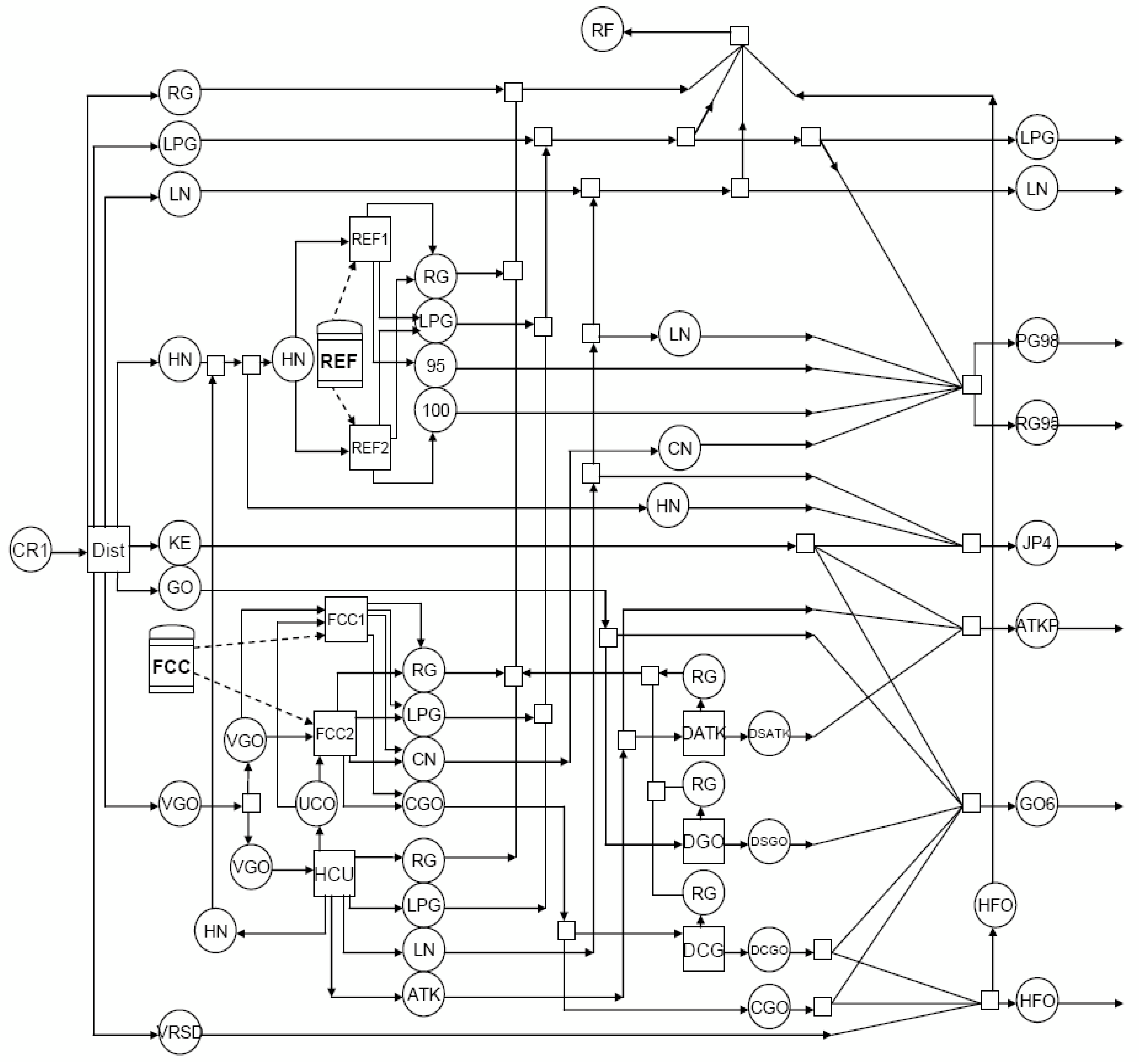
The oil refinery flow diagram considered in the case studies is shown in Figure 1, and the major unit capacity limits are shown in

Table 1. Capacities of different refinery units.

Unit	Capacity (kton/y)
Distillation	12,000
Reforming	2000
FCCU	1000
Hydrocracker	2000
Des Gas Oil	3000
Des Cycle Gas Oil	70
DATK	1200

FCCU and DATK stand for Fluid Cat Cracker and Des Aviation Turbine Kerosene, respectively.

. The planning period considered is one year, and the feedstock to the refinery is of a single type (e.g., Arabian light crude) with a total flow rate of 12,000 kton/y in order to produce different final products. These parameters are inspired by the work of Al-Qahtani [32], and further details about parametrization and the following results are available in Alnahdi [31].

The pollutants considered in this study are SO_x and NO_x, whereas CO₂ emission is incorporated into the analysis as a greenhouse effect. Several emission mitigation alternatives are considered. Among these, fuel switching represents switching from the current fuel (fuel oil) to natural gas. The SO_x capture process considered in this study is wet scrubber (WS) with fuel-gas desulphurization (FGD) technology, and the considered NO_x capture process is based on retrofitting current burners with low NO_x burner technology (will be denoted as LNB hereafter). For the CO₂ capture process, MEA absorption technology is considered.

CO₂ emissions parameters are estimated based on the work by Ritter et al. [33], whereas emissions data of the pollutants are based on Kassinis [34]. Cost parameters associated with fuel switching and MEA capture process are estimated based on the work by Elkamel et al. [35]; while, those associated with SO_x and NO_x capture processes are taken from a report by the World Bank [36].

Three scenarios are considered in this study in order to illustrate the validity of the model discussed in the previous section. For the first scenario, the process planning model in Section 2.1 is solved without any emissions mitigation, which is considered as the base case scenario. The second scenario is related to reducing one particular emission at a time (e.g., CO₂) without considering other emissions (e.g., SO_x and NO_x) using a special case of the model in Section 2.2. That is, each pollutant is reduced in an independent manner. Finally, the third scenario is related to the examination of reducing different emissions together in a general/dependent manner using the general model in Section 2.2.

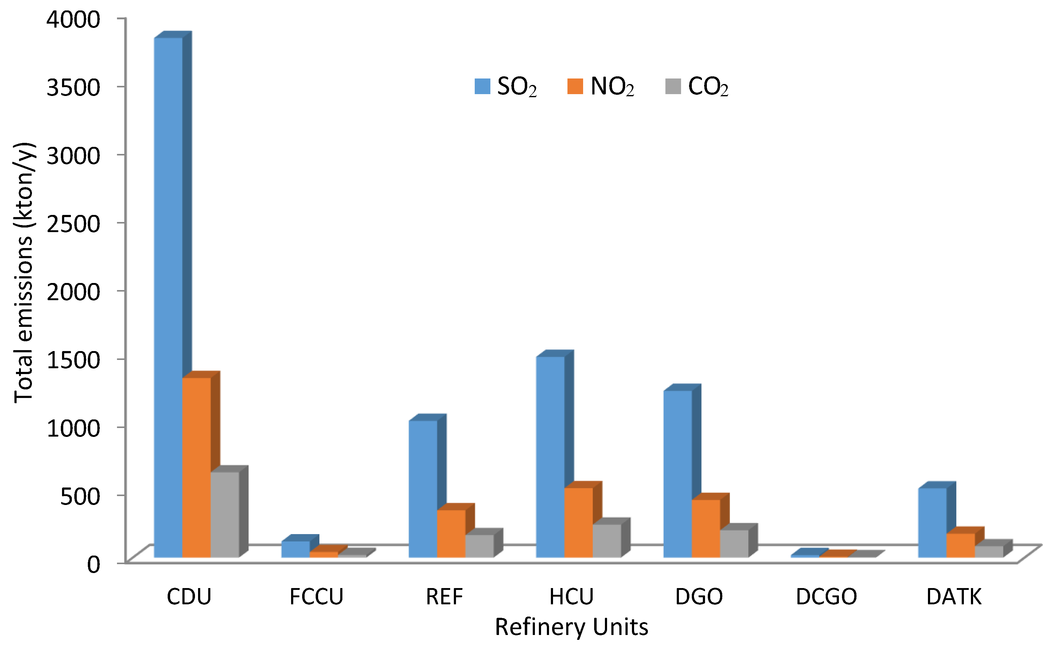
3.1.1. Results of Base Case Scenario

The objective of this base case scenario is to minimize the overall annualized cost minus the revenue from export while meeting the internal demand for each product with quality specifications. The market demands and specifications for different products that the refinery has to meet are shown in

Table 2. Domestic demand for final products.

Product	Demand (kton/y)
LPG	150
LN	90
PG98	30
PG95	1600
JP4	1300
GO6	2500
ATKP	1000
HFO	700

LPG: liquefied petroleum gas; LN: light naphtha; PG98: refinery gasoline with 98 octane number; PG95: refinery gasoline with 95 octane number; JP4: No. 4 jet fuel; GO6: No. 6 gas oil; ATKP: aviation turbine kerosene product; HFO: petroleum heating fuel oil;.

, and this is applied for all case studies. The emission results of the base case scenario, where no emission reduction plans are considered, are shown in Figure 3. These results imply a total annual production cost minus export revenue of $3,295,058 for the considered refinery. The total emissions from all the units for SO_x, NO_x, and CO₂ were 8170.6, 2826.9 and 1342.3 kton/y, respectively.

3.1.2. Results for Independent Emission Reduction

In this scenario, the focus is on reducing one emission at a time without considering the other pollutants, in order to analyze the impact of reducing each emission independently and to figure out the overall refinery cost correspondingly. Comparisons of cost increment when reducing SO_x, NO_x, and CO₂ emissions are given in

Table 3. SO_x emission reduction for different refinery units.

Reduction	Base Case	10%	20%	30%	40%	50%	60%
Unit 1	Emission Rate (kton/y)
CDU	3816.0	3434.4	3035.4	2760.0	2346.0	1904.4	1439.6
FCCU	119.3	107.3	85.5	89.6	76.2	61.8	57.7
REF	1005.7	905.1	714.4	702.3	597.0	484.6	314.1
HCU	1475.8	1328.3	1294.3	984.2	836.5	679.1	584.2
DGO	1226.0	1103.4	964.1	851.8	724.0	587.7	549.2
DCGO	18.8	16.9	21.1	11.0	9.4	7.6	7.2
DATK	508.8	457.9	429.0	339.3	288.4	234.1	239.3
Total Emission	8170.5	7353.4	6543.8	5738.1	4877.4	3959.3	3191.3
Cost ($/y)	3,295,058.9	3,302,704	3,338,273	3,360,812	3,415,168	3,486,346	3,513,680
Cost increase (%)	0.0	0.2	1.3	2.0	3.6	5.8	6.6

¹ Distillation (CDU), Reforming (REF), Fluid Cat Cracker (FCCU), Hydrocracker (HCU), Des Gas Oil (DGO), Des Cycle Gas Oil (DCGO), and Des Aviation Turbine Kerosene (DATK).

,

Table 4. NO_x emission reduction for different refinery units.

Reduction	Base Case	10%	20%	30%	40%	50%	60%
Unit 1	Emission Rate (kton/y)
CDU	1320.3	1188.3	1056.2	1031.2	1042.8	583.3	401.2
FCCU	41.3	37.1	33.0	42.4	17.7	16.3	14.6
REF	348.0	313.2	278.4	265.3	151.3	155.0	135.0
HCU	510.6	459.6	408.5	340.5	223.3	236.8	205.1
DGO	424.2	381.8	339.4	182.1	184.1	340.5	306.5
DCGO	6.5	5.9	5.2	4.3	2.3	1.6	1.2
DATK	176.0	158.4	140.8	117.4	77.0	81.6	69.1
Total Emission	2826.9	2544.2	2261.5	1983.2	1698.5	1415.1	1132.7
Cost ($/y)	3,295,058	3,311,068	3,338,273	3,465,016	3,503,746	3,510,880	3,522,880
Cost increase (%)	0.0	0.5	1.3	5.2	6.3	6.5	6.9

¹ Distillation (CDU), Reforming (REF), Fluid Cat Cracker (FCCU), Hydrocracker (HCU), Des Gas Oil (DGO), Des Cycle Gas Oil (DCGO), and Des Aviation Turbine Kerosene (DATK).

and

Table 5. CO₂ emission reduction for different refinery units.

Reduction	Base Case	10%	20%	30%	40%	50%	60%
Unit 1	Emission Rate (kton/y)
CDU	626.9	590.5	531.4	457.0	376.2	283.8	192.6
FCCU	19.6	18.6	16.8	14.4	13.1	14.6	7.7
REF	165.2	143.9	129.5	111.4	107.1	96.0	50.0
HCU	242.5	204.1	183.7	158.0	137.4	116.8	161.7
DGO	201.4	176.6	159.0	136.7	123.6	113.6	62.4
DCGO	3.1	4.9	4.4	3.8	2.1	1.9	1.4
DATK	83.6	70.4	63.3	54.5	47.4	40.3	55.7
Total Emission	1342.3	1208.9	1088.0	935.7	807.0	666.9	531.5
Cost ($/y)	3,295,058	3,311,068	3,338,273	3,360,812	3,379,316	3,397,771	3,515,168
Cost increase (%)	0.0	0.5	1.3	2.0	2.6	3.1	6.7

¹ Distillation (CDU), Reforming (REF), Fluid Cat Cracker (FCCU), Hydrocracker (HCU), Des Gas Oil (DGO), Des Cycle Gas Oil (DCGO), and Des Aviation Turbine Kerosene (DATK).

, respectively.

For the SO_x reduction scenario, it has been observed that with only a 6.6% increase in cost, almost 60% of SO_x releases can be alleviated by installing a wet scrubber capture process (WS) and/or through switching of fuels. On the other hand, NO_x discharge may be reduced by retrofitting the existing burners with LNB. There may be a maximum emissions reduction of 60% at a cost increment of 6.9% according to Table 4. The NO_x release is higher when no fuel switching was selected over the present fuel. Table 5 shows that a reduction of 60% of CO₂ emissions can be achieved in exchange for a 6.7% increase in cost. Furthermore, it has been observed that a decrease in the CO₂ discharge from 25% to 10% has been achieved without shifting units to the natural gas or by setting up extra MEA capturing practices. This decrease has been attained through load shifting, which is the recommended option for 10% emissions reduction target with a minor increase in cost. These scenarios demonstrate the flexibility of the model for proposing diverse emission reduction actions with different targets.

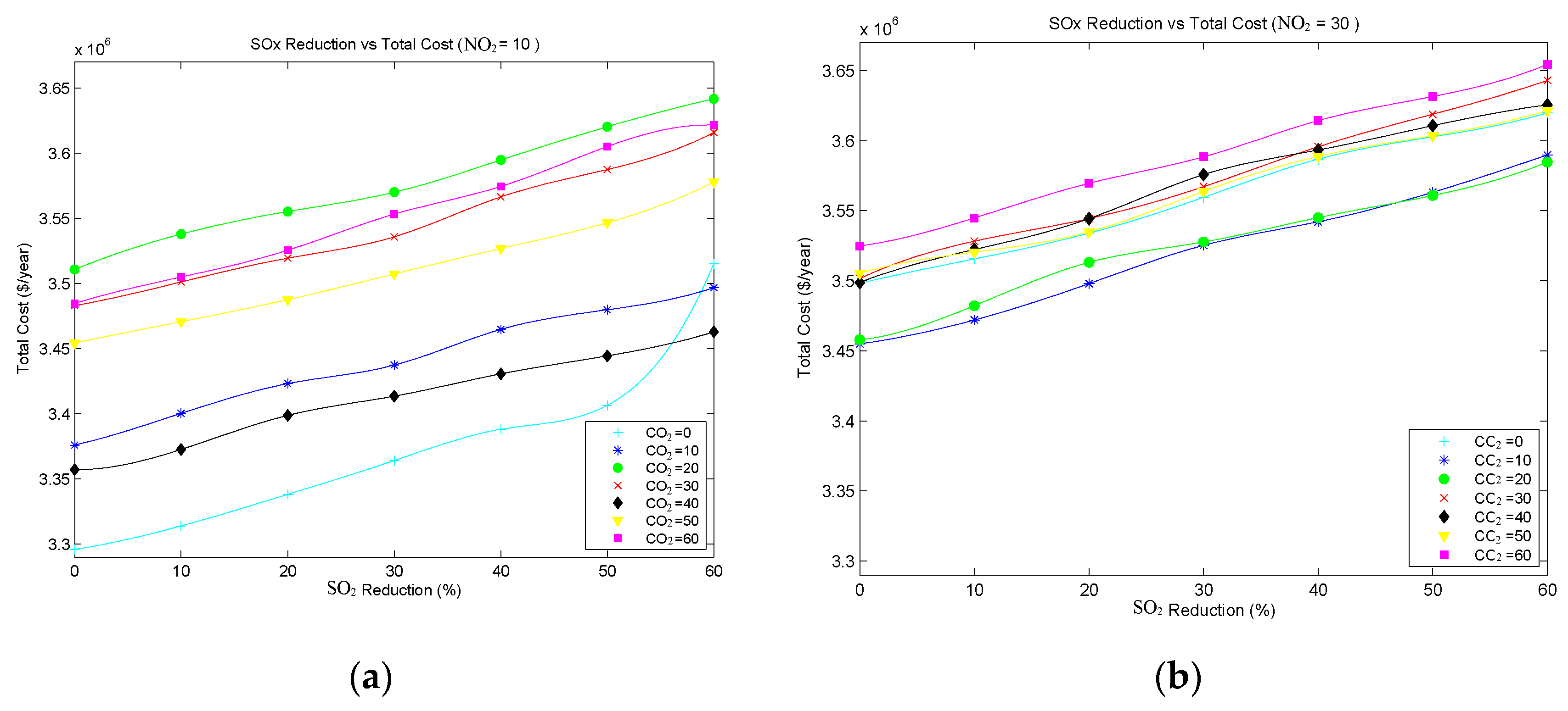
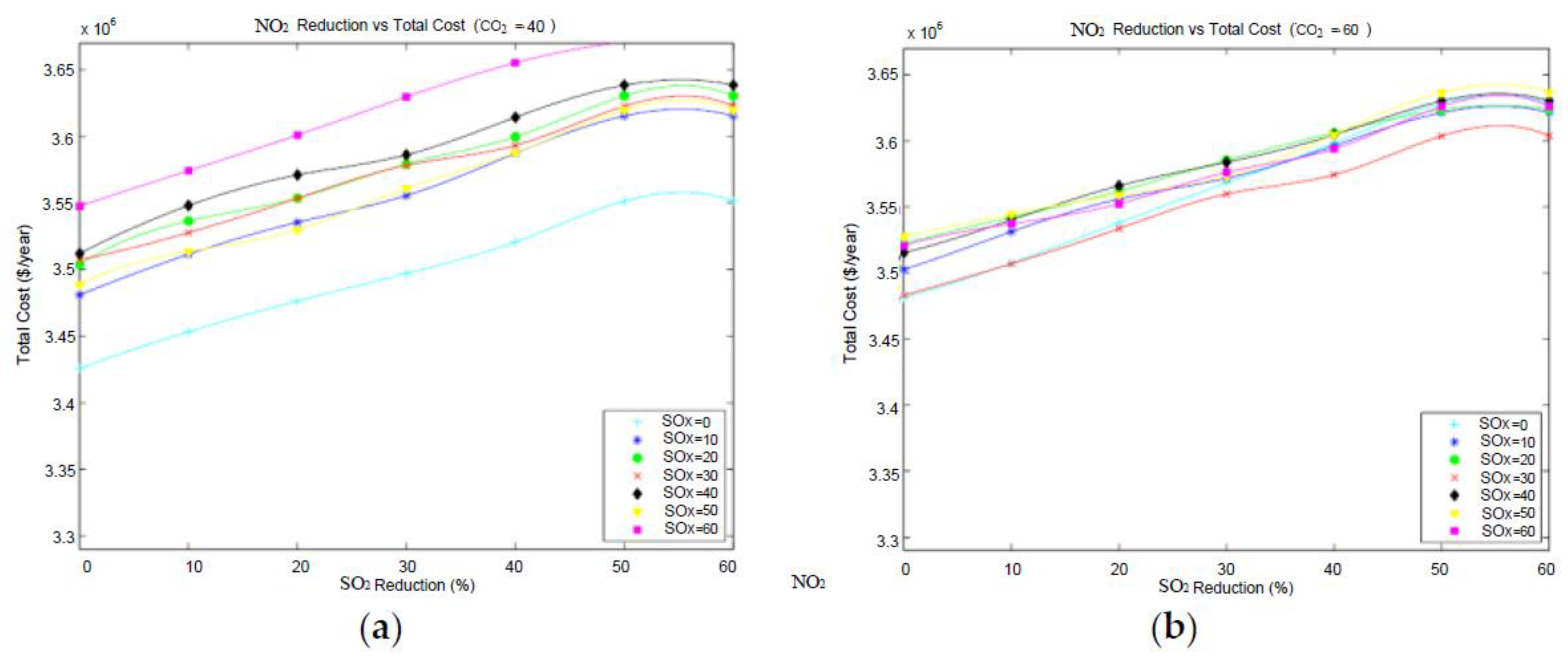
3.1.3. Results for Simultaneous Emissions Reduction

The goal here is to mitigate SO₂, NO₂, and CO₂ emissions simultaneously to various levels, and to compare the overall costs of the resulting mitigation plan.

Table 6. Cost comparison for different scenarios of simultaneous reduction in SO_x, NO_x, and CO₂ emissions.

Scenario	SOx (%)	NOx (%)	CO2 (%)	Total Cost	Cost Increase (%)
1	10	10	10	3,399,494	3.2
2	30	10	10	3,406,170	3.4
3	10	30	10	3,436,589	4.3
4	30	30	10	3,453,074	4.8
5	10	60	10	3,479,067	5.6
6	10	10	30	3,494,009	6.0
7	10	30	30	3,503,489	6.3
8	30	10	60	3,506,966	6.4
9	60	10	30	3,511,469	6.6
10	10	10	60	3,531,285	7.2
11	60	10	10	3,535,160	7.3
12	60	10	60	3,537,302	7.4
13	60	60	10	3,547,596	7.7
14	60	30	30	3,554,675	7.9
15	30	10	30	3,557,440	8.0
16	30	30	60	3,559,830	8.0
17	60	30	10	3,570,190	8.3
18	10	30	60	3,571,728	8.4
19	60	30	60	3,576,363	8.5
20	10	60	30	3,585,730	8.8
21	30	30	30	3,596,704	9.2
22	60	60	30	3,597,380	9.2
23	30	60	60	3,603,730	9.4
24	10	60	60	3,621,384	9.9
25	30	60	10	3,622,379	9.9
26	30	60	30	3,626,200	10.0
27	60	60	60	3,648,820	10.7

provides a summary of selected scenarios when varying reduction targets for all emissions including SO₂, NO₂, and CO₂ and the corresponding annual cost for each plan. For instance, reducing SO₂, NO₂, and CO₂ by 10%, 30%, and 60% each, results in increasing the annual cost by 3.2%, 9.2%, and 10.7%, respectively. Figure 4a and Figure 5b show the annual cost when reducing SO₂ from 0% to 60% with varying CO₂ and NO₂ reduction levels. These figures show that overall cost increases almost linearly with the emissions reduction level.

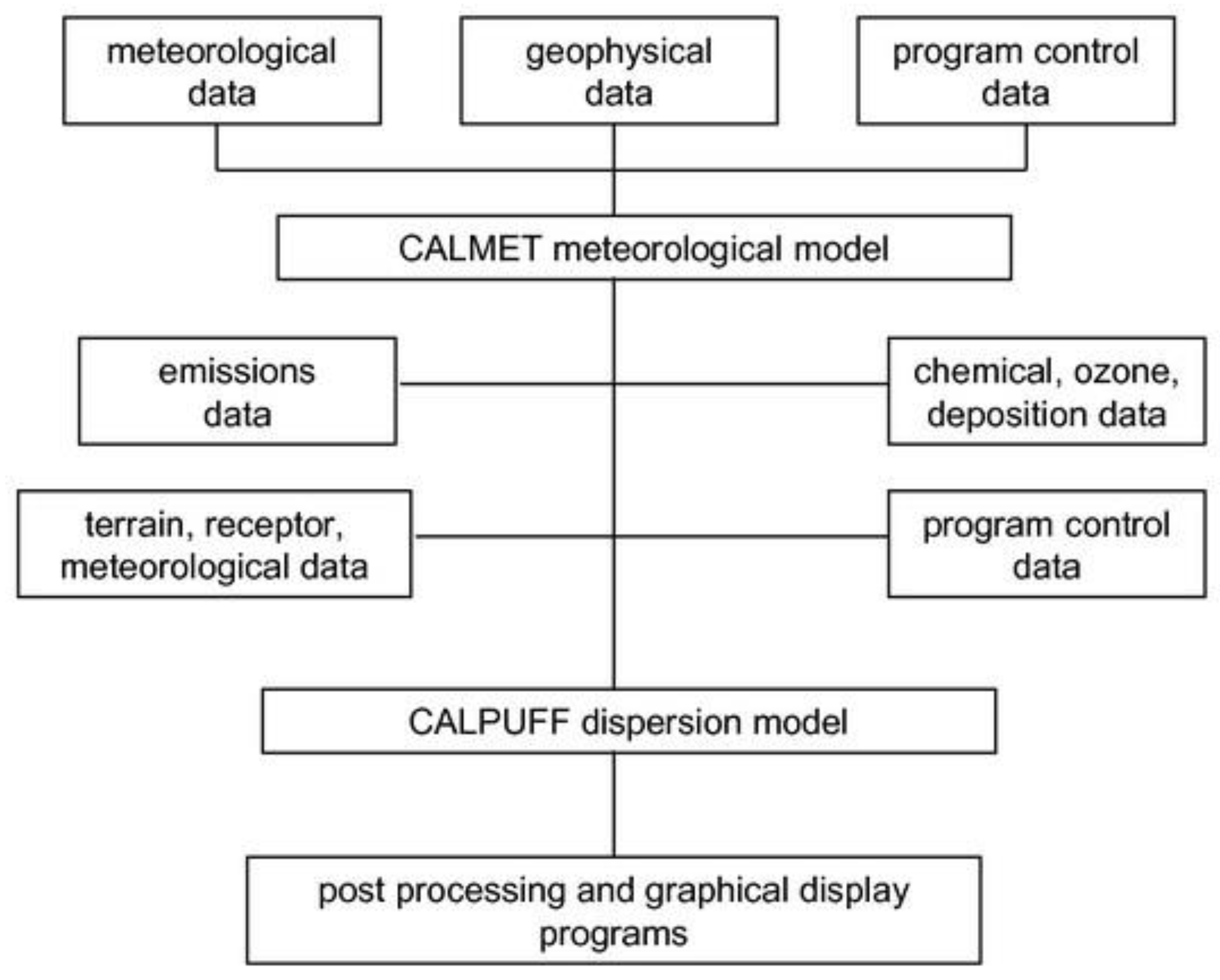
3.2. Case Study Details and Results for Air Pollution Dispersion

In this section, CALPUFF and SCREEN3 modeling tools are used to estimate the overall concentration of SO_x, NO_x, and CO₂ dispersed from an oil refinery site located in North Toronto, Ontario-Canada. This refinery has a similar process design to the one illustrated in Figure 1. The location of this refinery is 50 km away from the urban Toronto; thus, there is a need for a screening analysis gauging to what extent the emission from the refinery under the proposed mitigation strategies would affect the surrounding area.

The first step in air pollution analysis with CALPUFF model is identifying the meteorological domain information for the case study region, which is given in

Table 7. Meteorological domain information for the case study.

Parameter	North Toronto
Map projection	UTM
Latitude of origin	594.237 km
Longitude of origin	4877.678 km
Continent/Ocean	Global
Region	84
Datum code	WGS-84
X (Easting)	75 km
Y (Northing)	75 km
Number of X grid cells	75
Number of Y grid cells	75
Grid spacing	2 km
Number of vertical layers	10
Number cell face heights (m) 0, 20, 40, 80, 160, 320, 640, 1200, 2000, 3000

UTM: Universal Transverse Mercator.

. The surface data for the Toronto area were acquired from the weather records in the Canadian government website [37]. The surface stations were chosen based on their proximity to the source point and upper air stations. For each station, the hourly data includes the date, time, temperature, wind speed and direction, ceiling height, cloud cover, and station pressure. The hourly data for two modeling periods from (i) 1 January 2014 at 00:00 h to 31 January 2014 at 23:00 h; (ii) 1 May 2014 at 00:00 h to 31 May 2014 at 23:00 h were extracted and organized in a certain layout that is suitable for use in ‘SMERGE’ to create a formatted file ‘SURF.DAT’, which is compatible for usage with CALMET. The relevant surface station data is shown in

Table 8. Surface station data for the North Toronto area.

Parameter	North Toronto
Station Name	Toronto Buttonville
Latitude	43 51 44
Longitude	79 22 12
Elevation	198.1
Climate ID	615HMAK
WMO ID	71639
The Climate	ID YKZ

WMO: World Meteorological Organization.

.

The meteorological data of the upper air for the location was obtained from the radiosonde station records in the National Oceanic and Atmospheric Administration (NOAA) Earth System Research Laboratory (NOAA/ESRL) radiosonde database [38]. These data records contain the station ID number, date and time, and information of the sounding level followed by pressure, temperature, elevation, and wind direction and speed for each sounding level. The hourly data for the Toronto area was taken from one radiosonde station that is close to the study site for the two modeling periods mentioned above and was then prepared in a format suitable to use in “READ62” to generate the “UP.DAT” file that was used in the CALMET program. The relevant information about the radiosonde station is shown in

Table 9. Meteorological data for Radiosonde Station.

Parameter	North Toronto
Station name/location	Moosone PQ
UTM latitude	51.27
UTM longitude	80.65
X location on grid	808.3 km
Y location on grid	1 km
Elevation	10 m
WBAN	15,803
WMO ID	71,836

WMO: World Meteorological Organization; WBAN: Wireless Body Area Network; UTM: Universal Transverse Mercator.

. The geophysical data such as land use and terrain were obtained from the website of Geographic Information Systems [39], and used as input files in CTG-PROC and TERREL to produce “LU.DAT” and “TERREL.DAT”, respectively. All this data is compressed by a MAKEGEO program to generate the output file ‘GEO.DAT’, which was used in the CALMET program.

The proposed mathematical model in Section 2.2 was used to find the pollutant emission rates for the case study. The source parameters for the case study are shown in

Table 10. Source parameters for the case study.

Source Parameters	North Toronto
X coordinate (km)	592.430
Y coordinate (km)	4877.631
Base elevation (m)	256.6
Stack height (m)	75
Stack diameter (m)	6
Exit velocity (m/s)	20
Exit temperature (K)	418

. For different reduction plans, the emission rates of the three pollutants are given in

Table 11. Emission rates of different pollutants used in CALPUFF model for different reduction plans.

Reduction	Base Case	10%	20%	30%	40%	50%	60%
C O2 (kton/y)	1342.3	1208.1	1087.3	978.5	880.7	792.6	713.4
NOx (kton/y)	2826.9	2544.2	2289.8	2060.8	1854.7	1669.3	1502.3
SOx (kton/y)	8170.6	7353.5	6618.2	5956.4	5360.7	4824.7	4342.2

, which were used in the CALPUFF model and specified for the two modeling periods.

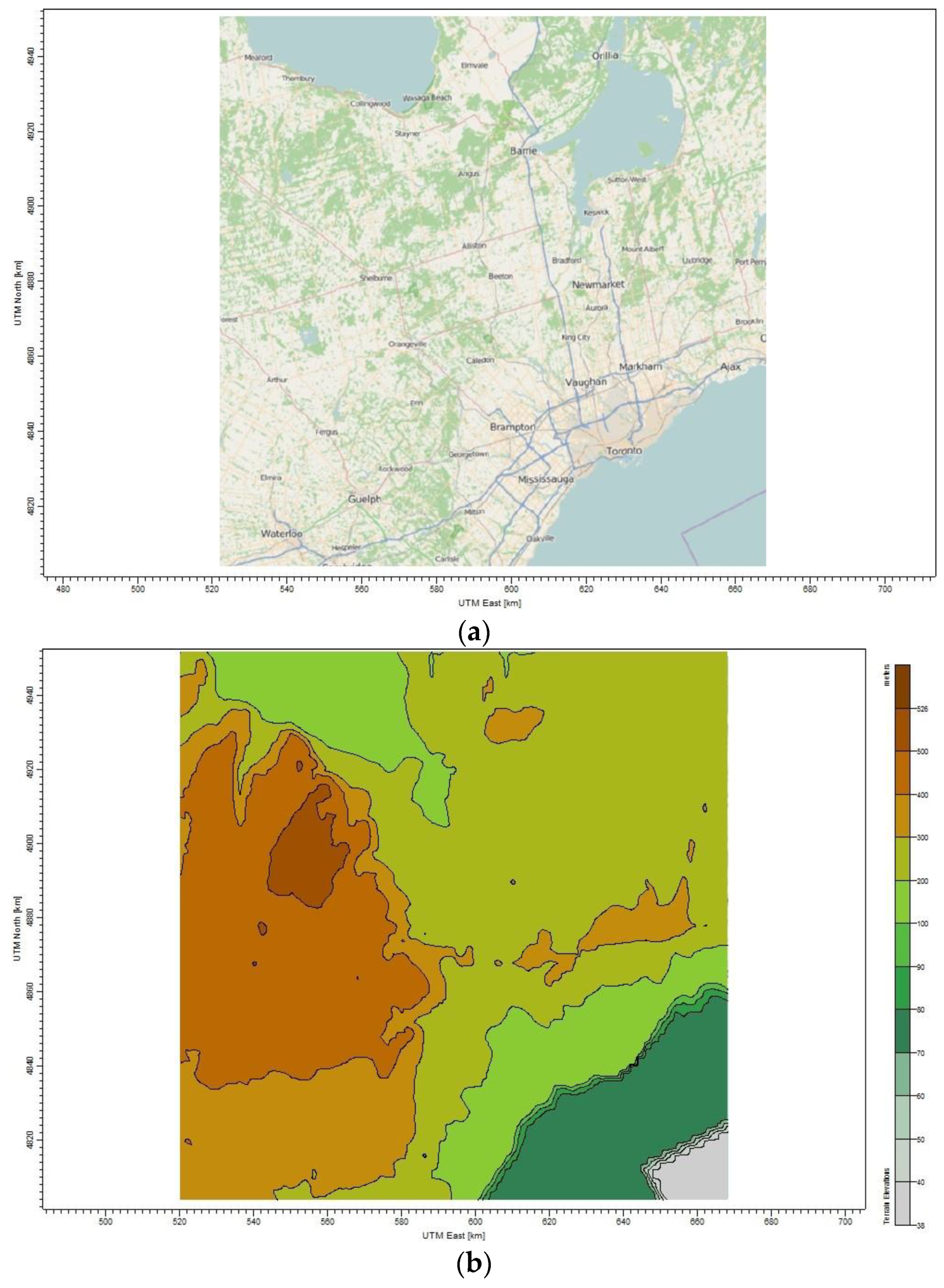
Initially, the CALPUFF model was used to estimate the pollutant concentrations emanated from the oil refinery over the surrounding region for a two-month modeling period of January and May of 2014. The CALPOST post-processor was used to determine their spatial distribution. Figure 6 presents the characteristics of the study area along with the ability of the CALPUFF model to simulate the geographical condition of the area of interest.

Table 12. The range of average CO₂ concentrations in January 2014 under the optimal production and emission control strategies for various targeted emission reduction levels.

Reduction Plan	Maximum Monthly Average Concentration µg/m3	Minimum Monthly Average Concentration µg/m3
Base Case	216	2
10%	194	2
30%	157	2
40%	141	1
50%	127	1
60%	115	1

illustrates the maximum and minimum monthly average concentrations of CO₂ for January 2014.

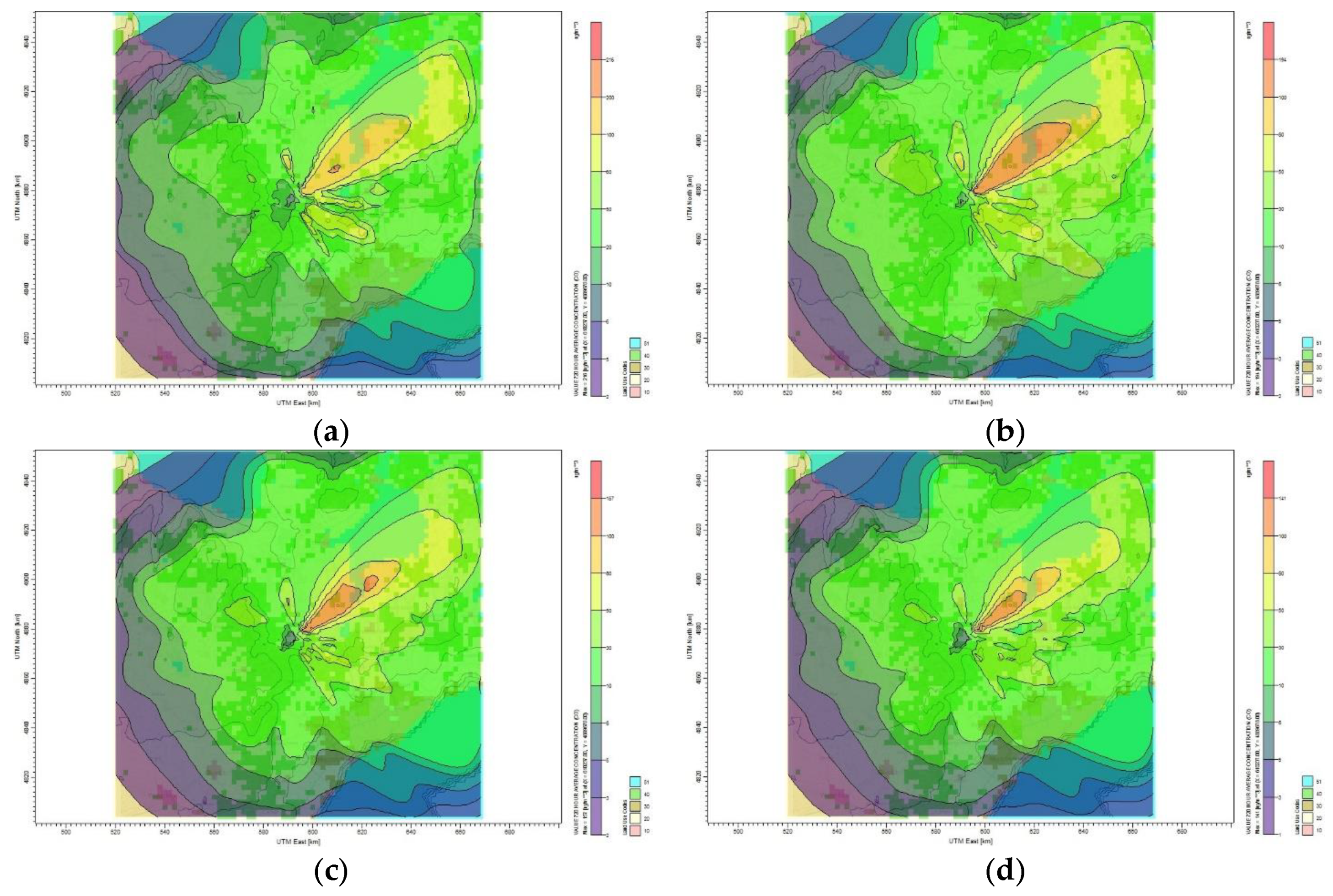
Figure 7 shows the CO₂ plume distributed significantly in the Toronto area in January 2014. The highest monthly CO₂ concentration calculated by CALPUFF view model is 216 µg/m³ and the lowest is 2 µg/m³ when considering the base case scenario as shown in Figure 7a. The plume affecting Toronto residential area concentration is 20 µg/m³. For the 10% reduction target, the maximum monthly average concentration of CO₂ was 194 µg/m³, and the minimum average concentration was 2 µg/m³, as seen in Figure 7b. The pollutant is dispersed in all the directions, especially in the northwest direction as seen in Figure 7c. For the 50% reduction target of CO₂, the maximum monthly concentration was 127 µg/m³ at a distance of 2 km from the source, as shown in Figure 7e. The dispersion of CO₂ was heading significantly in the south and northeast direction as presented in Figure 7d, thus affecting people in that area. As displayed in Figure 7f, the plume dispersed significantly towards the northwest and it shows that the maximum monthly average concentration of CO₂ obtained for 60% reduction target reached 115 µg/m³ within 2 km northeast of the source. It is clear how the plumes are covering the Toronto residential area with the plumes concentration ranging from 216 to 1 µg/m³ represented by the color code.

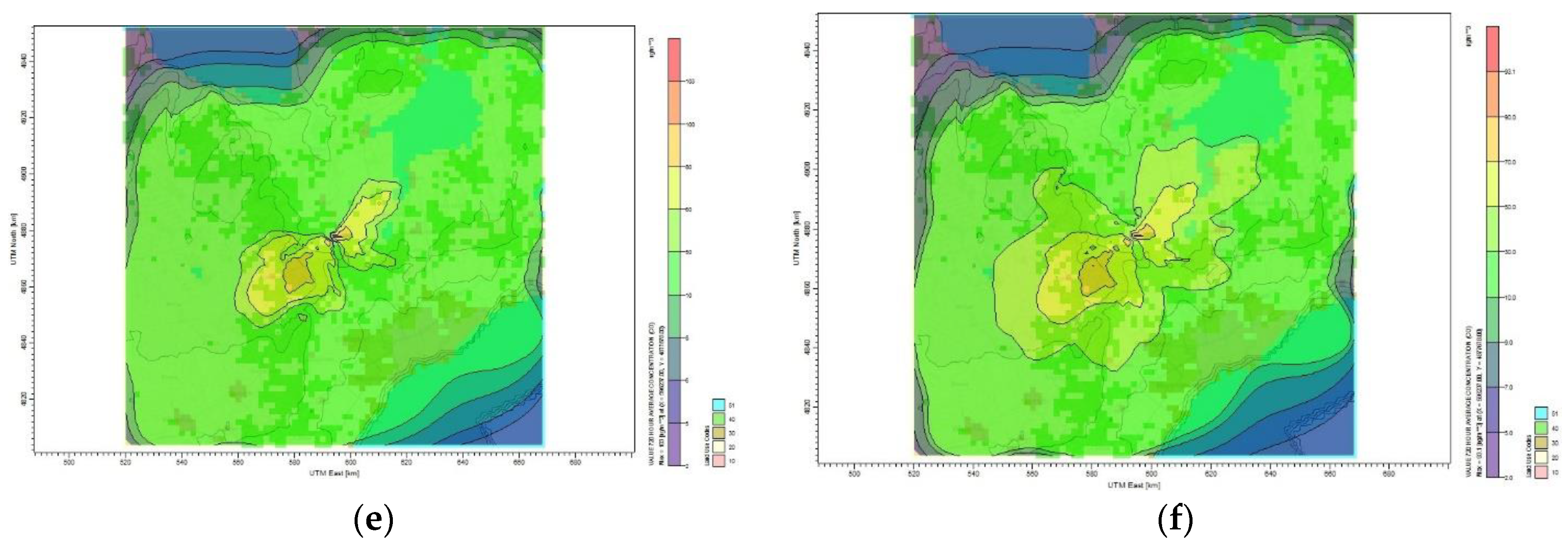
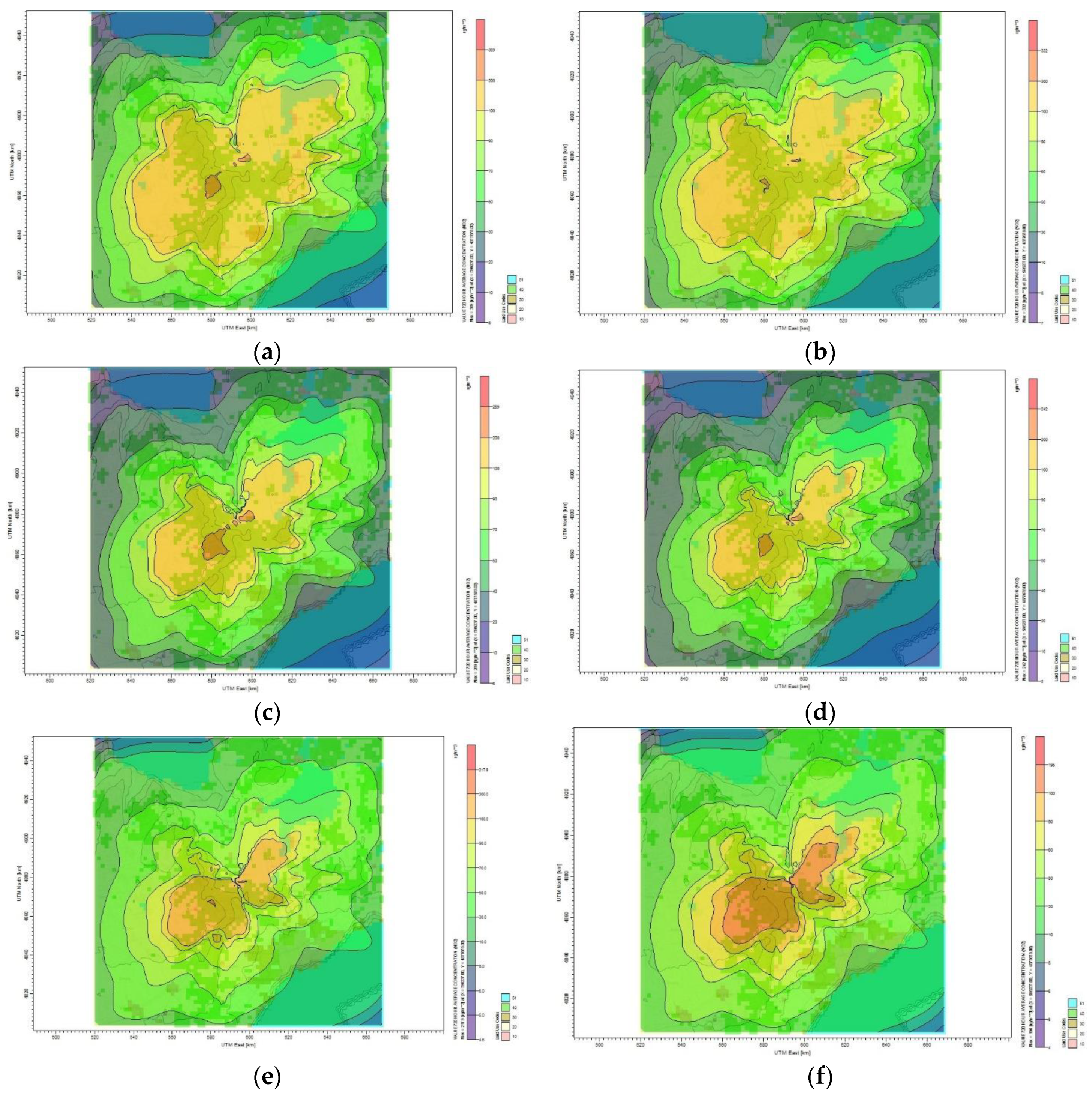
For the second period of May 2014,

Table 13. The range of average CO₂ concentrations in May 2014 under the optimal production and emission control strategies for various targeted emission reduction levels.

Reduction Plan	Maximum Monthly Average Concentration µg/m3	Minimum Monthly Average Concentration µg/m3
Base Case	175	4
10%	158	3
30%	128	3
40%	115	2
50%	103	2
60%	93.1	2

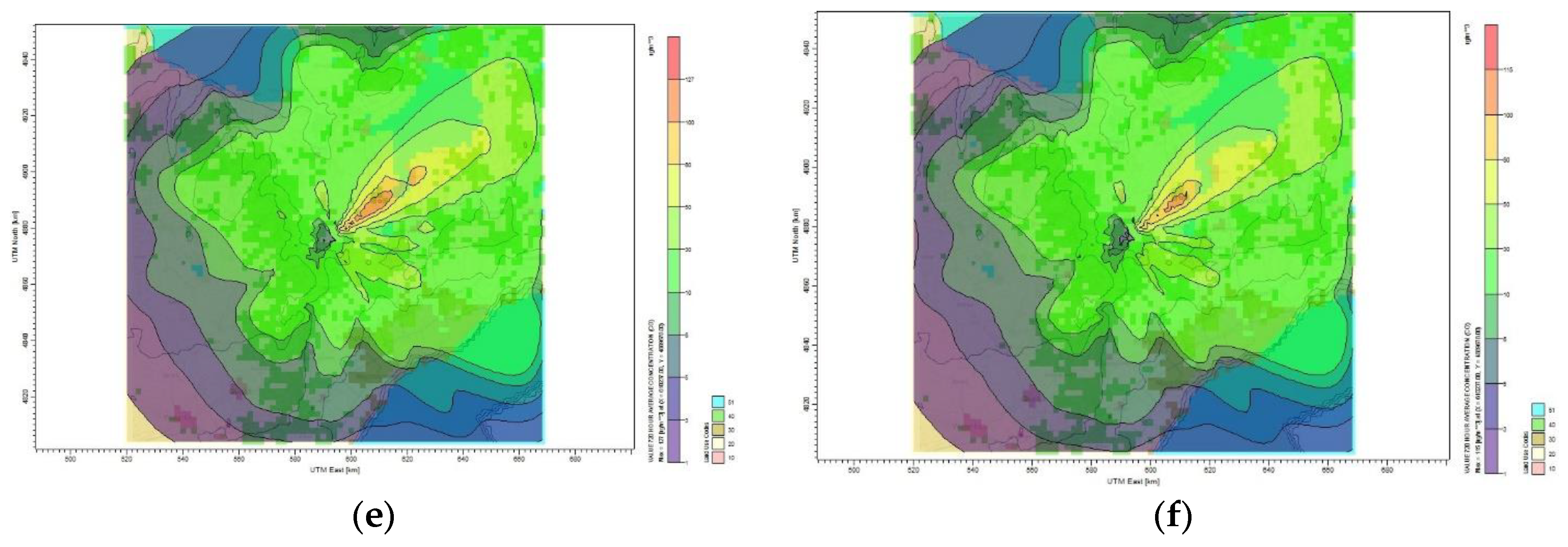
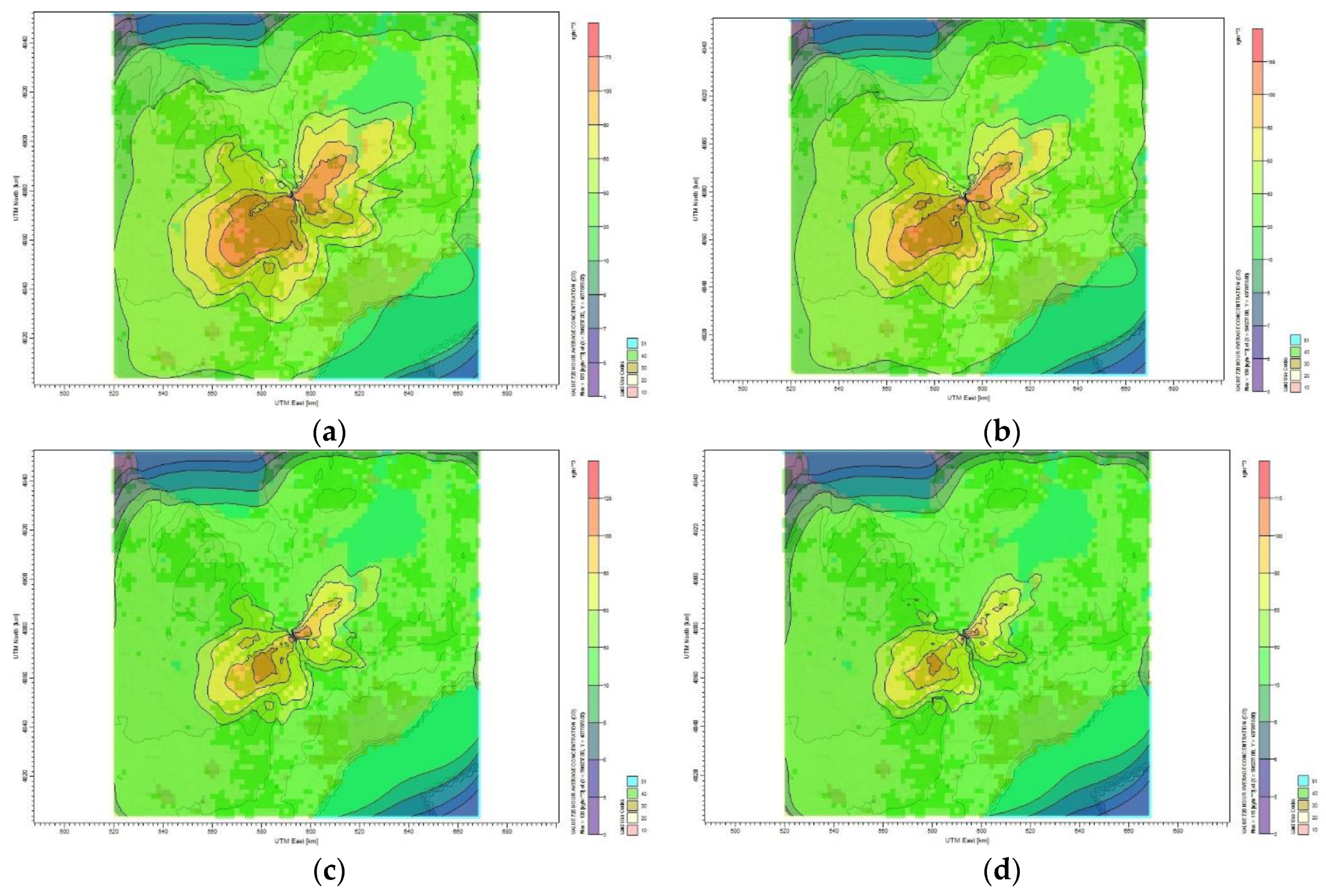
shows the maximum and minimum monthly average concentrations of CO₂ for the six reduction plans. Figure 8 shows the dispersion of CO₂ emission to the surrounding area of Toronto for different mitigation plans. The maximum monthly CO₂ concentration calculated by the CALPUFF model for the base case scenario is 175 µg/m³ and the lowest is 4 µg/m³. The plume affecting the Toronto residential area has a concentration of 20 µg/m³, as shown in Figure 8a. The maximum CO₂ monthly average concentration became 158 µg/m³ once the oil refinery site reduces its emission by 10%, as shown in Figure 8b. For the case of 30% CO₂ reduction, Figure 8c shows that the maximum average concentration reduced to 128 µg/m³ and the minimum concentration became 3 µg/m³. Furthermore, Figure 8f shows that reducing the CO₂ emission by 60% results in reducing the monthly average concentration to 93.1 µg/m³. The maximum monthly average concentration of CO₂ for all reduction plans that affect the Toronto area is between 2 and 30 µg/m³. No health symptoms are associated with this range of concentration values according to air quality standard and guideline [40].

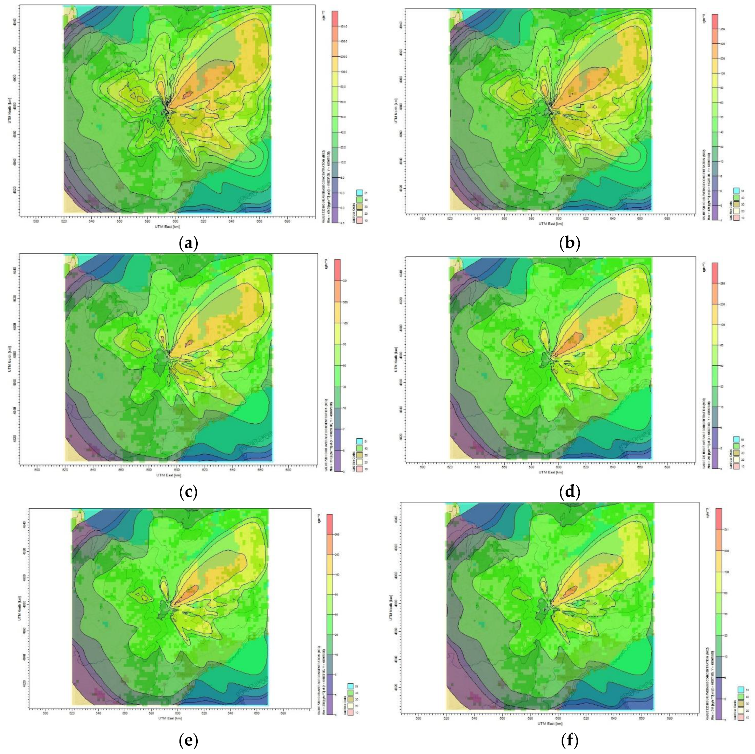
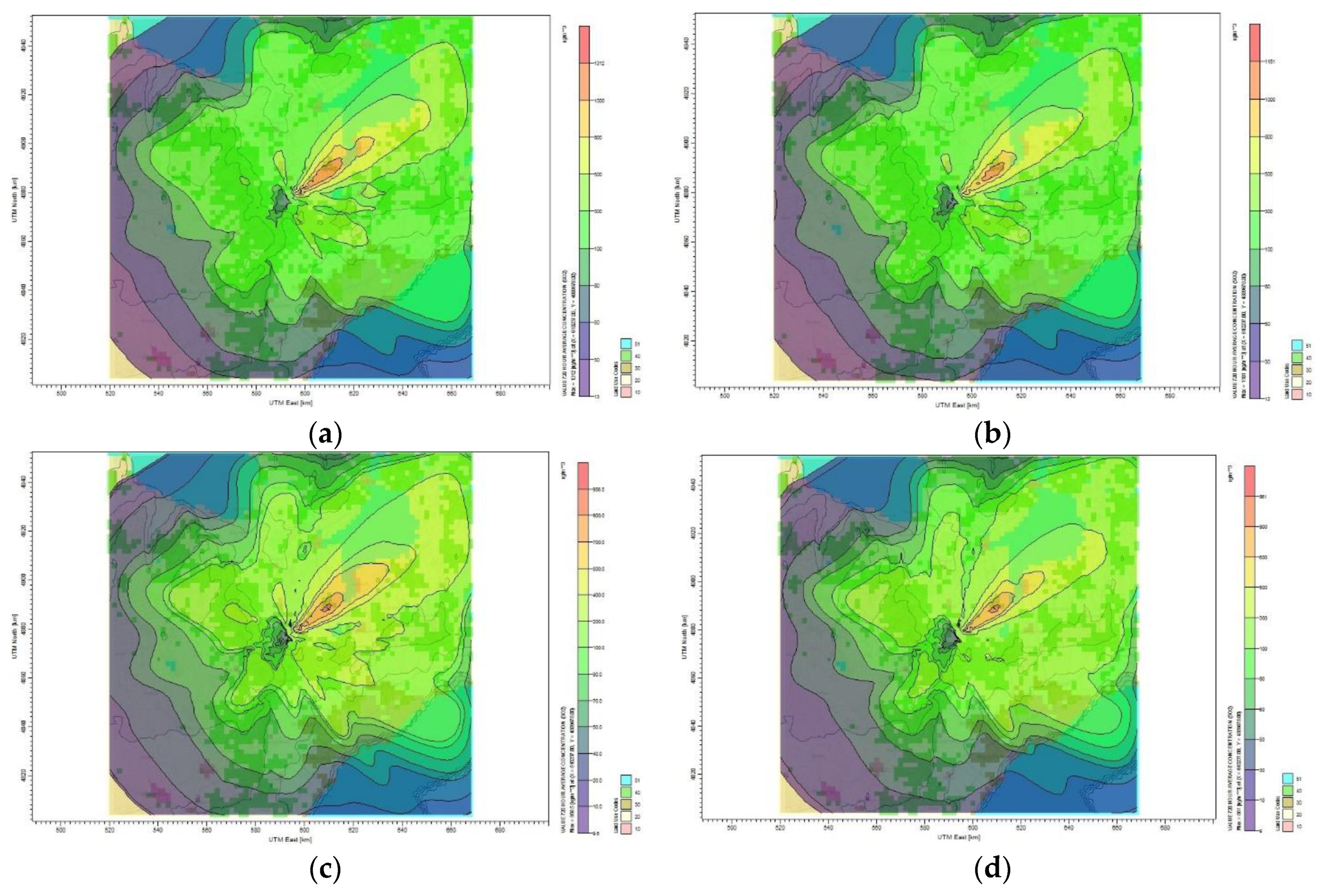
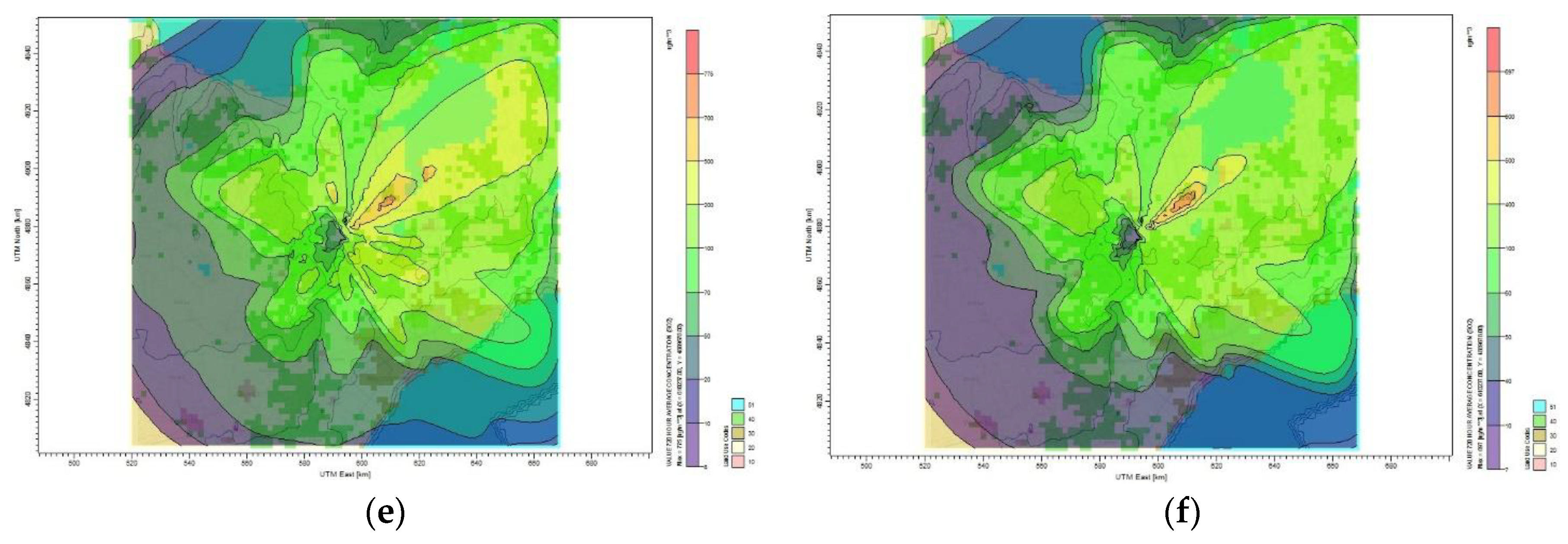
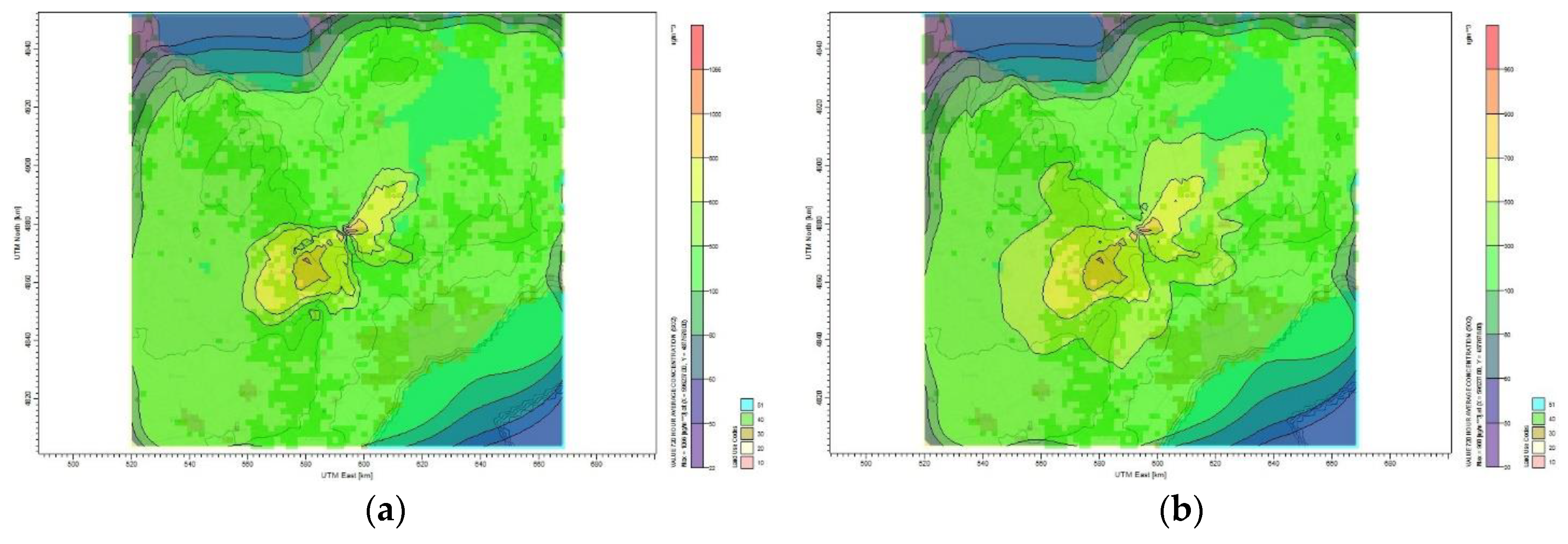
Similarly, the following set of results are related to the dispersion of SO_x and NO_x for the periods of January and May 2014, the tables and figures for which are excluded here for brevity and can be found in Appendix B. For January 2014, the maximum monthly average concentration of SO₂ when no reduction plan is applied to the refinery was 1312 µg/m³ and the plumes dispersed 5 km northeast of the source. The maximum and minimum average monthly concentrations of SO₂ were 1181 and 12 µg/m³ for 10% reduction target. It was observed that when the pollutants from the source were reduced by certain percentages, the concentration of the pollutants in the receptor area reduced accordingly. Therefore, reducing the SO₂ by 30%, 50%, and 60% results in reducing the maximum monthly average concentration to 956.5, 775, and 697 µg/m³, respectively. For May 2014, the maximum and minimum monthly average concentrations of SO₂ are 1066 and 22 µg/m³ for the base case scenario, whereas the plume affecting the Toronto residential area has a concentration of 100 µg/m³. Reducing 10% of SO₂ in the oil refinery decreases the maximum and minimum monthly average concentration of SO₂ to 960 and 20 µg/m³, respectively. The highest monthly SO₂ concentration computed by CALPUFF when reducing the SO₂ emission by 30% is 777 µg/m³ and the lowest is 16 µg/m³. The monthly concentration of plume covering the Toronto residential area is 80 µg/m³.

For January 2014, the maximum NO₂ concentration for the oil refinery was about 454 µg/m³ when no reduction plan was applied. For the 10% reduction plan, it was observed that NO₂ was dispersed from the northwest to the northeast of the Toronto area with maximum and minimum monthly average concentrations of 409 and 4 µg/m³, respectively. The maximum monthly average concentration of NO₂ for the plant was about 331 µg/m³ when reducing the emission by 30%. The monthly average of SO₂ concentration for 40%, 50%, and 60% reduction plans was 298, 268, and 241 µg/m³, respectively. For May 2014, the maximum monthly average concentration of NO₂ was 332 µg/m³ for the 30% reduction plan.

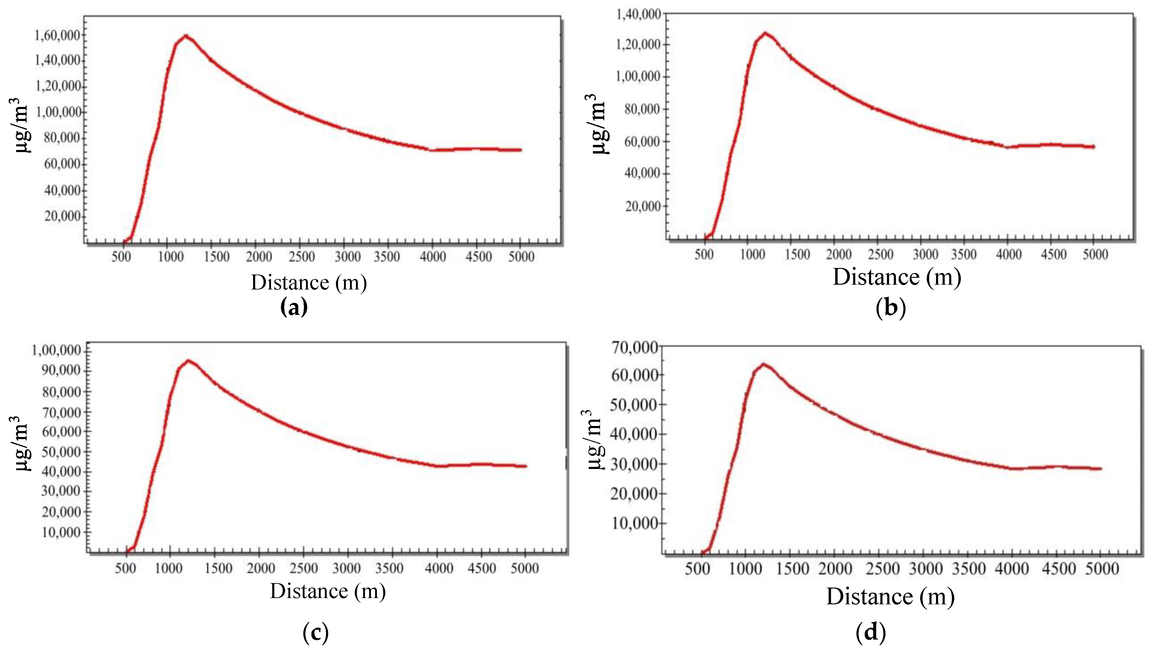
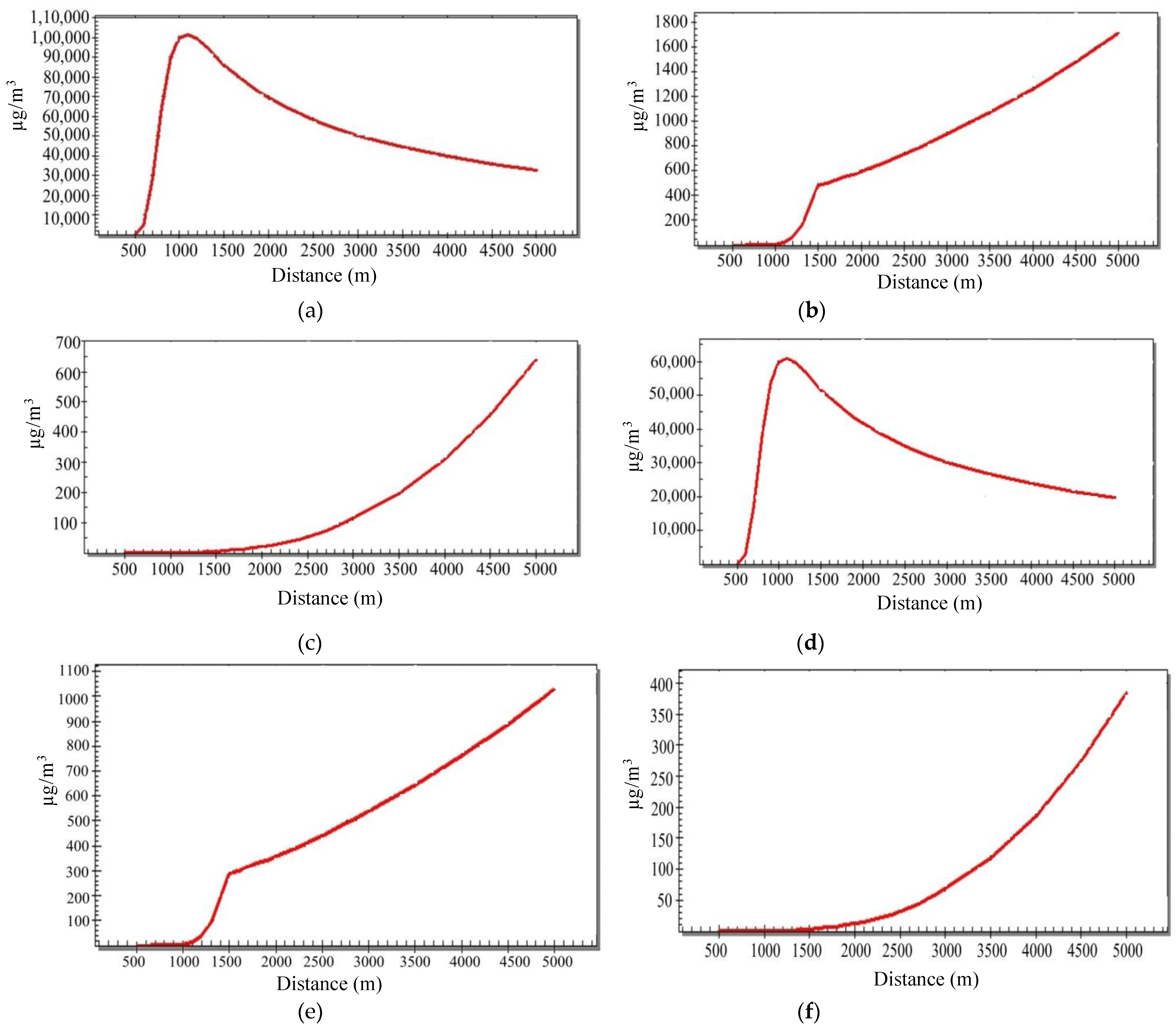
For SCREEN3, the input data used is for the atmospheric emission rates of SO_x, NO_x, and CO₂ from the oil refinery. The results of SCREEN3 are expressed in concentration units (µg/m³) and distance (m). The simulations were performed considering the option of ‘full meteorology’; that is, defining the type of atmospheric stability class where the program assumes the ‘C’ class was omitted. The maximum concentration was calculated for SO_x for the base case and various mitigation plans. In all scenarios, the maximum concentration was found at 1200 m away from the source and the emission concentrations were 1.6 × 10⁵, 1.3 × 10⁵, 9.5 × 10⁴, and 6.4 × 10⁴ µg/m³ for the base case, 20%, 40%, and 60% reduction plans, respectively.

4. Conclusions

This study addresses the problem of selecting the best pollution control strategies for an oil refinery given specific values of emission reduction targets. The problem has been formulated MINLP based on three mitigation options and chooses the optimal set to meet a certain emission reduction goal with the minimum annual cost minus export revenues, while ensuring the satisfaction of the demand levels and quality specifications. The model was illustrated on an industrial scale refinery case study, considering three pollutants (SO_x, NO_x, and CO₂) with different mitigation alternatives of fuel switching and capturing pollutants. The results showed that with only a 6.6% increment in price, almost 60% of SO_x releases can be alleviated by installing a wet scrubber capture process WS and through switching of fuels. Furthermore, reducing NO_x by 60% increases the cost by 6.9%. Our results showed that a reduction of 60% of CO₂ emissions can be gained in exchange for a 6.7% increase in the total cost. Nevertheless, when three pollutants considered together, reducing SO_x, CO_x, and NO_x emission by 60% simultaneously requires a 10.7% increase in cost.

This comparison illustrates that emission rates can be reduced with reasonable cost using the aforementioned strategies in an industrial-scale facility. However, emission reduction strategies should be analyzed collectively for all considered pollutants. This is because the strategies for individual pollutants may not be the same and the strategy for one pollutant may not achieve the desired effect on the others. As indicated our results, decreasing the emission of all three pollutants would be close to 40% (e.g., (10.7−6.6%)/10.7%) more expensive. Therefore, relying on an independent analysis of each pollutant could be quite misleading.

Furthermore, two air dispersion models are used to investigate the dispersion of the pollutants released from a potential oil refinery located in North Toronto, Ontario, Canada, whose production and emission reduction strategies are designed based on the proposed optimization model. The reported estimations of pollutant concentrations, dispersion, and transport from CALPUFF and SCREEN3 verified that the optimal production and pollution control plans derived by the proposed MINLP model may significantly reduce the CO₂, SO_x, and NO_x emission around the area of study significantly. These results show that mathematical programming and dispersion models can be used simultaneously to derive efficient and effective production and pollution control plans for oil refineries.

References

1. Environment Canada. Canada’s Greenhouse Gas Inventory. Available online: https://www.canada.ca/en/environment-climate-change/services/climate-change/greenhouse-gas-emissions/inventory (accessed on 10 August 2015).
2. Kyoto Protocol. United Nations framework convention on climate change (UNFCCC). In Kyoto Protocol to the United Nations Framework Convention on Climate Change; UNFCCC: Kyoto, Japan, 1998. [Google Scholar]
3. Figueroa, J.D.; Fout, T.; Plasynski, S.; McIlvried, H.; Srivastava, R.D. Advances in CO2 capture technology: The US department of energy’s carbon sequestration program. Int. J. Greenh. Gas Cont. 2008, 2, 9–20. [Google Scholar] [CrossRef]
4. Olajire, A.A. CO2 capture and separation technologies for end-of-pipe applications—A review. Energy 2010, 35, 2610–2628. [Google Scholar] [CrossRef]
5. Shepard, D.S. A load shifting model for air pollution control in the electric power industry. J. Air Pollut. Cont. Assoc. 1970, 20, 756–761. [Google Scholar] [CrossRef]
6. Nevers, N.D. Air Pollution Control Engineering; Waveland Press: Long Grove, IL, USA, 2010. [Google Scholar]
7. Red Tape Reduction Action Plan. Canadian Cost-Benefit Analysis Guide: Regulatory Proposals. Available online: http://www.tbs-sct.gc.ca/rtrap-parfa/analys/analystb-eng.asp (accessed on 10 August 2015).
8. Xing, Y.Z.; Guo, H.; Feddes, J.; Yu, Z.; Shewchuck, S.; Predicala, B. Sensitivities of four air dispersion models to climatic parameters for swine odor dispersion. Trans. ASABE 2007, 50, 1007–1017. [Google Scholar] [CrossRef]
9. Cimorelli, A.J.; Perry, S.G.; Venkatram, A.; Weil, J.C.; Paine, R.J.; Wilson, R.B.; Lee, R.F.; Peters, W.D.; Brode, R.W. AERMOD: A dispersion model for industrial source applications. Part I: General model formulation and boundary layer characterization. J. App. Meteorol. 2005, 44, 682–693. [Google Scholar] [CrossRef]
10. Scire, J.S.; Strimaitis, D.G.; Yamartino, R.J. A User’s Guide for the CALPUFF Dispersion Model; Earth Tech Inc.: Concord, MA, USA, 2000. [Google Scholar]
11. Wesely, M.L.; Doskey, P.V.; Shannon, J.D. Deposition Parameterizations for the Industrial Source Complex (ISC3) Model; Argonne National Lab: Argonne, IL, USA, 2002.
12. Shewchuk, S.; Guo, H.; Xing, Y. The Use of Air Quality Dispersion Models for Validation of Operational Setback Distances near Intensive Livestock Operations. Confidential Report for Environment Canada 2006; SRC Publication: Durham, NC, USA, 2006; p. 12072-1. [Google Scholar]
13. Guidelines of Air Quality Dispersion Modeling in British Columbia (GAQDMBC); British Columbia Ministry of Environment: Victoria, BC, Canada, 2008. Available online: https://www.for.gov.bc.ca/hfd/library/documents/bib97377.pdf (accessed on 10 August 2015).
14. Sullivan, J.E.; Dix, D.; Brown, D.L. MPCA Air Dispersion Modeling Practices; Minnesota Pollution Control Agency (MPCA): Saint Paul, MN, USA, 2002; Available online: https://www.pca.state.mn.us/sites/default/files/aq2-58.pdf (accessed on 10 August 2015).
15. Casey, K.D.; Bicudo, J.R.; Schmidt, D.R.; Anshu, S.; Gay, S.W.; Gates, R.S.; Jacobson, L.D.; Hoff, S.J. Air Quality and Emissions from Livestock and Poultry Production/Waste Management Systems; ASABE Publication: St. Joseph, MI, USA, 2006; Available online: http://www.abe.iastate.edu/adl/files/2011/10/Air-Quality-White-Paper.pdf (accessed on 10 August 2015).
16. Bluett, J.; Gimson, N.; Fisher, G.; Heydenrych, C.; Freeman, T.; Godfrey, J. Good Practice Guide for Atmospheric Dispersion Modelling; Ministry for the Environment: Wellington, New Zealand, 2004.
17. Steyn, D.G.; Trini-Castelli, S. Air Pollution Modeling and Its Application XXI; Springer: Dordrecht, The Netherlands, 2012. [Google Scholar]
18. Wispelaere, C.D.; Gryning, S.E. Air Pollution Modeling and Its Application; Plenum Press: New York, NY, USA, 1981. [Google Scholar]
19. Abdul-Wahab, S.; Chan, K.; Ahmadi, L.; Elkamel, A. Impact of geo-physical and meteorological conditions on the dispersion of NO2 in Canada. Air Qual. Atmos. Health 2014, 7, 113–129. [Google Scholar] [CrossRef]
20. Acute Exposure Guideline Levels (AEGLs) for Ethylamine; U.S. Environmental Protection Agency: Washington, DC, USA, 2008. Available online: https://www.epa.gov/sites/production/files/2014-08/documents/ethylamine_tsd_interim_version_106_2008.pdf (accessed on 10 August 2015).
21. Guo, H.; Feddes, J.; Dehod, W.; Laguë, C.; Edeogu, I. Monitoring of odour occurrence in the vicinity of swine farms by resident observers-Part II: Impact of weather conditions on odour occurrence. Can. Biol. Eng. 2006, 48, 23–29. [Google Scholar]
22. Schmitz, R. Modelling of air pollution dispersion in Santiago de Chile. Atmos. Environ. 2005, 39, 2035–2047. [Google Scholar] [CrossRef]
23. Sercu, B.; Peixoto, J.; Demeestere, K.; Elst, T.V.V.; Langenhove, H.V. Odors treatment: Biological technologies. In Odors in the Food Industry; Springer: Boston, MA, USA, 2006; pp. 125–158. [Google Scholar]
24. De Melo, A.M.V.; Santos, J.M.; Mavroidis, I.; Reis, N.C., Jr. Modelling of odour dispersion around a pig farm building complex using AERMOD and CALPUFF. Comparison with wind tunnel results. Build. Environ. 2012, 56, 8–20. [Google Scholar] [CrossRef]
25. Air Quality Model Guideline (AQMG). Alberta Environment and Sustainable Resource Development: Edmonton, AB, Canada, 2013. Available online: https://open.alberta.ca/publications/9781460105993 (accessed on 10 August 2015).
26. Ainslie, B.; Jackson, P.L. The use of an atmospheric dispersion model to determine influence regions in the Prince George BC air shed from the burning of open wood waste piles. J. Environ. Manag. 2009, 90, 2393–2401. [Google Scholar] [CrossRef] [PubMed]
27. Yeomans, H.; Grossmann, I.E. A systematic modeling framework of superstructure optimization in process synthesis. Comput. Chem. Eng. 1999, 23, 709–731. [Google Scholar] [CrossRef]
28. Al-Qahtani, K.; Elkamel, A. Multisite refinery and petrochemical network design: Optimal integration and coordination. Ind. Eng. Chem. Res. 2009, 48, 814–826. [Google Scholar] [CrossRef]
29. Al-Qahtani, K.Y.; Elkamel, A. Planning and Integration of Refinery and Petrochemical Operations; Wiley-VCH: Weinheim, Germany, 2010; ISBN 978-3-527-32694-5. [Google Scholar]
30. Brooke, A.; Kendrick, D.; Meeraus, A. GAMS Release 2.25: A User’s Guide; GAMS Development Corporation: Washington, DC, USA, 1996. [Google Scholar]
31. Alnahdi, A. Economical and Environmental Impacts of Emission Mitigation in Petroleum Refineries. Master’s Thesis, University of Waterloo, Waterloo, UK, 2015. [Google Scholar]
32. Al-Qahtani, K.Y. Petroleum Refining and Petrochemical Industry Integration and Coordination under Uncertainty. Ph.D. Thesis, University of Waterloo, Waterloo, UK, 2009. [Google Scholar]
33. Ritter, K.; Nordrum, S.; Shires, T.; Lev-On, M. Ensuring consistent greenhouse gas emissions estimates. Chem. Eng. Prog. 2005, 101, 30–37. [Google Scholar]
34. Kassinis, G.I. A model for estimating pollution emissions for individual economic activities. Environ. Impact Assess. Rev. 1998, 18, 417–438. [Google Scholar] [CrossRef]
35. Elkamel, A.; Ba-Shammakh, M.; Douglas, P.; Croiset, E. An optimization approach for integrating planning and CO2 emission reduction in the petroleum refining industry. Ind. Eng. Chem. Res. 2008, 47, 760–776. [Google Scholar] [CrossRef]
36. Maternal Mortality in 2005: Estimates Developed by WHO, UNICEF, UNFPA and the World Bank; World Health Organization: Geneva, Switzerland, 2007; Available online: https://www.who.int/whosis/mme_2005.pdf (accessed on 10 August 2015).
37. Historical Climate Data; Government of Canada. Available online: http://climate.weather.gc.ca (accessed on 10 August 2015).
38. NOAA/ESRL Radiosonde Database. Available online: esrl.noaa.gov/raobs/ (accessed on 10 August 2015).
39. Geographic Information Systems Resource. Available online: www.webgis.com (accessed on 10 August 2015).
40. WHO Air Quality Guidelines for Particulate Matter, Ozone, Nitrogen Dioxide, and Sulfur Dioxide - Global Update 2005; World Health Organization: Geneva, Switzerland, 2006; Available online: http://whqlibdoc.who.int/hq/2006/WHO_SDE_PHE_OEH_06.02_eng.pdf (accessed on 10 August 2015).
Figure 1. A schematic diagram of the refinery using state-equipment network (SEN) representation (adapted from Elkamel and Al-Qahtani [28], see Appendix A for details).
Sustainability 11 03771 g001
Figure 2. CALPUFF Modeling System (Adapted from Scire et al. [10]).
Sustainability 11 03771 g002
Figure 3. Total emissions from different refinery units (Distillation (CDU), Reforming (REF), Fluid Cat Cracker (FCCU), Hydrocracker (HCU), Des Gas Oil (DGO), Des Cycle Gas Oil (DCGO), and Des Aviation Turbine Kerosene (DATK)).
Sustainability 11 03771 g003
Figure 4. Cost comparison for reduction in SO2: (a) at NO2 = 10; (b) at NO2 = 30.
Sustainability 11 03771 g004
Figure 5. Cost comparison for reduction in NO2: (a) at CO2 = 40; (b) at CO2 = 60.
Sustainability 11 03771 g005
Figure 6. Characteristics of the study area: (a) street view; (b) terrain view.
Sustainability 11 03771 g006
Figure 7. CO2 dispersion around North Toronto for January 2014: (a) base case; (b) 10% reduction; (c) 30% reduction; (d) 40% reduction; (e) 50% reduction; (f) 60% reduction.
Sustainability 11 03771 g007aSustainability 11 03771 g007b
Figure 8. CO2 dispersion around North Toronto for May 2014: (a) base case; (b) 10% reduction; (c) 30% reduction; (d) 40% reduction; (e) 50% reduction; (f) 60% reduction.
Sustainability 11 03771 g008aSustainability 11 03771 g008b