An Exploratory Multivariate Statistical Analysis to Assess Urban Diversity

Abstract

Understanding diversity in complex urban systems is fundamental in facing current and future sustainability challenges. In this article, we apply an exploratory multivariate statistical analysis (i.e., Principal Component Analysis (PCA) and Multiple Factor Analysis (MFA)) to an urban system’s abstraction of the city’s functioning. Specifically, we relate the environmental, economical, and social characters of the city in a multivariate system of indicators by collecting measurements of those variables at the district scale. Statistical methods are applied to reduce the dimensionality of the multivariate dataset, such that, hidden relationships between the districts of the city are exposed. The methodology has been mainly designed to display diversity, being understood as differentiated attributes of the districts in their dimensionally-reduced description, and to measure it with Euclidean distances. Differentiated characters and distinctive functions of districts are identifiable in the exploratory analysis of a case study of Barcelona (Spain). The distances allow for the identification of clustered districts, as well as those that are separated, exemplifying dissimilarity. Moreover, the temporal dependency of the dataset reveals information about the district’s differentiation or homogenization trends between 2003 and 2015.

1. Introduction

It is expected that 66% of the world population will be urban by 2050 [1]. This on-going urbanization process entails major environmental and socioeconomic impacts that compromise the function and stability of cities. As complex systems, cities generate interesting patterns and trends that are neither easily described nor predicted [2]. Systems that produce complexity consist of diverse rule-following entities of which the behaviors are interdependent [3,4]: Those entities interact over a contact structure or network, and they often adapt (i.e., by learning in a social system or by natural selection in an ecological one) [5]. Due to their adaptive behavior and complexity, cities have been also identified as centers for economic development, productivity, creativity, innovation, and cultural transformation [6,7,8]. In this scenario, understanding cities’ complexity will play a key role in facing current and future sustainability challenges at the regional and global scales [9,10,11].

One of these challenges will be to improve the resilience of cities [12,13,14,15,16], and this is not straightforward since one action may not give the expected transformation of the complex system. Resilience refers to the ability of a system to adapt to a modifying process while retaining its functionality and not necessarily returning to the previous equilibrium state [17,18,19]. This definition comes from the non-equilibrium paradigm of ecology [17] and fits the complexity and uncertainty inherent to cities, as it includes adaptation as a key process that cannot be easily predicted. Specifically, urban resilience has been defined by Meerow et al. [16] as “the ability of an urban system—and all its constituent socio-ecological and socio-technical networks across temporal and spatial scales—to maintain or rapidly return to desired functions in the face of a disturbance, to adapt to change, and to quickly transform systems that limit current or future adaptive capacity”. This definition comprises the three pathways to a resilient state: persistence, transition, and transformation [20]. To some extent, measuring resilience is tightly related to inspecting the property of the system to remain functional over time—from persistence to adaptation—and hence, to sustain itself. In any case, there are five questions that need to be addressed during the planning of effective resilience policy in a city: Who? Resilience for whom? Who benefits with that strategy?; What? Which part of the city is going to be more resilient?; When? Is the policy oriented to face short-term disruptions or long-term stress?; Where? Is the policy limited to a spatial scale? Is it portraying cross-scalar interactions?; and Why? What is the goal of the program [21].

We are interested in the relationship between diversity and resilience in the urban system and in the effects of diversity fostering resilience, basically, in the development of a statistical framework to evaluate urban systems, which may be helpful in the formulation of urban policy and in answering these questions. When we speak about diversity, we refer to any of the three characteristics of a population [5]: (1) diversity within a type or variation in some attribute (such as differences in the length of finches’ beaks); (2) diversity of types and kinds or species in biological systems (such as different types of stores in a mall); and (3) diversity of composition, which refers to differences in configuration (such as different connections between atoms in a molecule). The diversity concept has characterized populations or collections of entities like ecosystems, with multiple types of flora and fauna, but it is also suitable to be applied in cities, having different types of people, organizations, infrastructural systems, etc. Regardless that the influence of diversity in the stability of a system is still a controversial issue [5,22,23], a number of studies in socio-ecological systems have pointed out a positive correlation between diversity and resilience [12,24,25,26,27]. From an urban ecology perspective, it is argued that cities with higher levels of environmental, economic, and social diversity have a higher resilience capacity [13,14,25]. This argument relies on the assumption that a highly diverse system possesses many different entity types and, therefore, a bunch of individuals belonging to these different types that are able to perform similar functions at a wider range of conditions—response diversity— [13,24]. Furthermore, it has been shown that diversity is a fundamental property that ensures the city’s functionality in the face of disturbances; it is an essential factor for economic growth, attractiveness, and liveability of cities [6]. In the last decade, some scholars have supported this thesis by arguing that diversity fosters productivity, innovation, and therefore economic development in cities [28,29,30].

From a formal perspective, the assessment and characterization of a system’s diversity have been increasingly performed by means of a multiplicity of variables instead of aggregated attributes. This has been motivated by the enormous increase of computer power and accessibility to open datasets in recent years. However, direct interpretation of multivariate information is not easy and some level of aggregation is required to display an integrated picture of the system: Aggregated measures surely reduce the amount of information, highlight patterns, and enhance the communication of results. Nevertheless, gathering all the information into one single diversity index is usually not convenient for the following reasons. Firstly, most of the methods for aggregating indicators into indices produce a disconnection between the more intuitively original variables and the quantities resulting from these indices [31]. Secondly, aggregation also requires some form of human judgment so it relies on potentially distorting assumptions [31,32]. Lastly, aggregate indices (e.g.,variance, information entropy, or phylogenetic distances [5]) barely capture interactions within complex systems [32].

Here, we explore diversity in urban complex systems through multivariate statistical methods (i.e., Principal Component Analysis (PCA) and Multiple Factor Analysis (MFA)). These techniques are robust methodologies in the sense that they provide a moderate trade-off between the large volume of initial data and its final aggregation. In this regard, PCA [33,34] is probably the most widely used multivariate statistical technique. It has been applied in urban geography since the 1970s to analyze the landscape change [35,36,37], but it has lately emerged as a meaningful statistical tool to understand the geographical complexity of globalization processes [38], sustainable development [32,39,40,41], and socioeconomic resilience trends [42]. At the urban scale, it has been used to identify urban typologies—of neighborhoods or cities—in metropolitan areas. By identifying typologies, these studies have exhibited—to some extent—the degree of diversity of the urban systems, being described by several socioeconomic variables (i.e., race, ethnicity, age, family structure, education, employment, and income) [43,44,45]. MFA [46,47], on the other hand, is a multivariate data analysis technique—an extension of PCA—for summarizing and visualizing complex data, where variables are organized into groups of variables: It reveals an integrated picture displaying the relationship between observations and groups of variables [33,46,48]. MFA has been applied mostly in sensory analysis; see for example the recent work of References [49,50,51,52]. In the urban context, few studies have applied MFA [53,54].

The way to measure diversity with these methods is explained by their capacity to reduce the dimensionality of the multivariate dataset by transforming the original data of correlated variables into a set of a few representative variables—known as principal components—that extract the most relevant information [34,55]. The objective is to visualize the relations between the system’s components, such that, the more differentiated entities, the more diversity indication. Since distanced results in the dimensionally reduced description indicate diverse attributes of districts as described by the multivariate system of indicators, we may seek to expose those differentiated results: One basic visualization method is the plot of variables and individuals in relation with the principal components (i.e., biplot). Another is the quantitative measurement of such differences with Euclidean distances.

In this paper, we apply a descriptive multivariate statistical analysis (i.e., PCA and MFA) to an urban system’s abstraction of the city’s functioning. Specifically, we relate the environmental, economical, and social characters of the city of Barcelona (Spain) in a multivariate system of indicators by collecting measurements of those variables at the district scale. We analyze diversity qualitatively and quantitatively by means of the dimensionality reduction of the dataset and the recognition of interactions and patterns among districts. The main purpose of this work is to exhibit the diversity of the urban system since—in a broader sense—we are interested in its relationship with resilience. In this sense, the temporal span of the dataset—from the year 2003 to the year 2015—not only brings a wider and reliable perspective to the city’s description but also allows for a temporal analysis: It constitutes the main tool to understand diversity trends and to identify key points towards the achievement of resilience. We also apply MFA to expose relations between urban metabolism groups of variables and the principal components.

This article is organized as follows. In Section 2, we present our case study, the multivariate dataset, and the statistical techniques that we apply to expose diversity. The results of the multivariate statistical methods are presented in Section 3. A discussion is given next in Section 4. The paper ends with some conclusions and future research inquiries in Section 5.

2. Materials and Methods

In this section, we present the statistical methodology for exposing diversity in the urban system. For doing so, the case study is described in the first part of the section. Then, we introduce the main hypothesis and transform the city into an abstraction of multiple variables that allows us to quantify diversity. Finally, the implemented statistical techniques are presented in the last part of this section.

2.1. Case Study

Barcelona city—our case study—can be studied at its largest scale or as a composition of smaller divisions. The choice of the scale influences the overall interpretation of diversity: Cities may seem diverse on one scale, but when looking at another scale, it may appear homogeneous. At its largest scale, Barcelona has a population of approximately 1.6 million inhabitants living in $102.16$ km${}^2$ (15,865 inhabitants per km${}^2$) [56]. We choose to represent the city at the district scale with the aim of revealing particular functions and patterns of these urban subsystems while covering efficiently most of the city’s territory.

Since 1987, Barcelona has been divided into 10 administrative districts which can be compared with neighborhoods in a common metropolitan area. Our selection of districts—and therefore, of the city’s representation—ends up with Ciutat Vella, Eixample, Les Corts, and Gràcia as our case study. These districts are chosen to characterize Barcelona since the surface covered by the case study comprises a total area of $22.06$ km${}^2$ and represents $22\%$ of the total city’s surface, as shown in Figure 1. With respect to population, the case study comprises 571,183 inhabitants, accounting for $35\%$ of the city’s population.

We also consider the following criteria in our selection: urban form, socioeconomic characteristics of the population, age of urban development—year or period of establishment and proximity to the city center—distance to historic center, and type of urban planning—organic or planned.

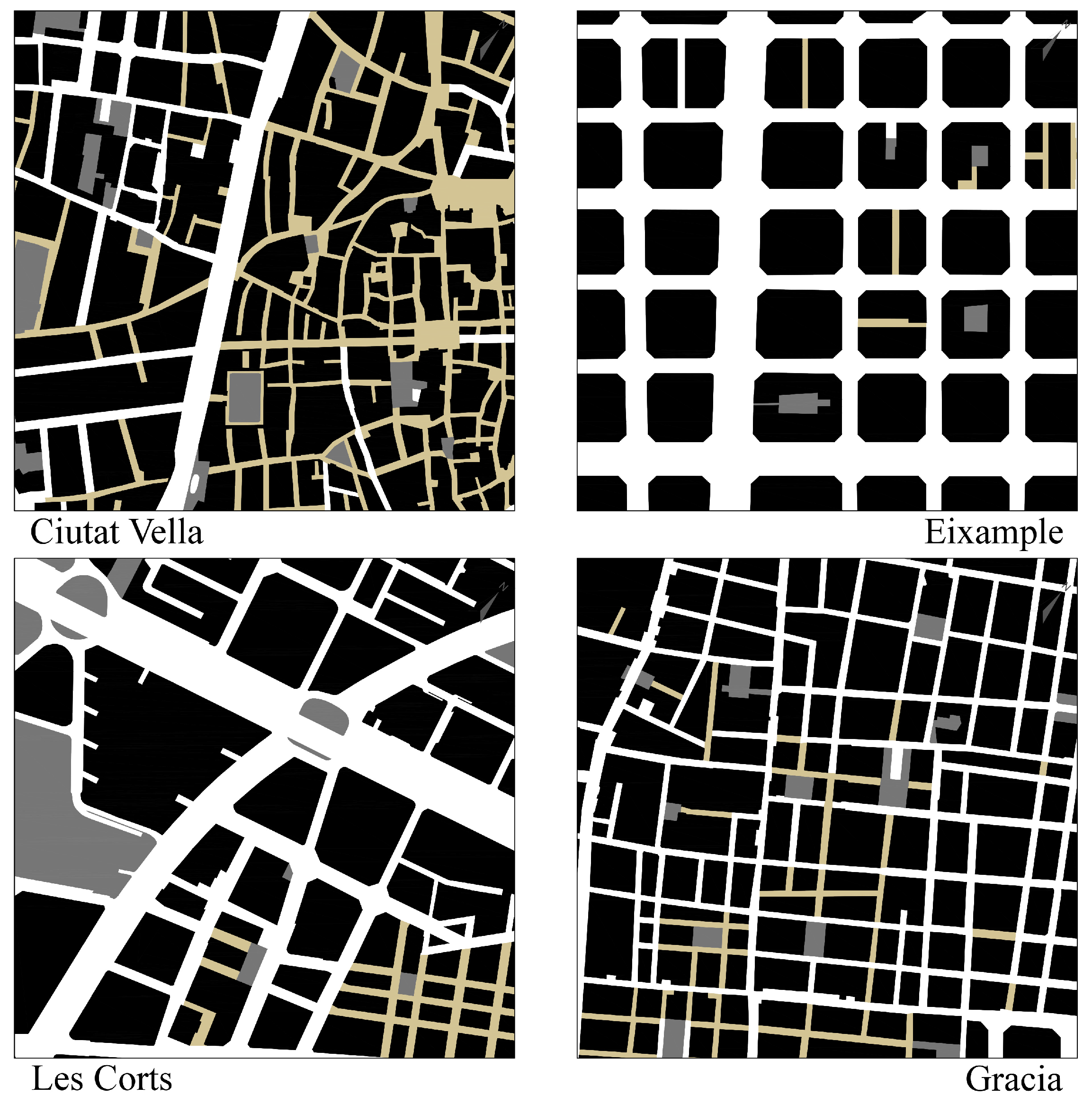
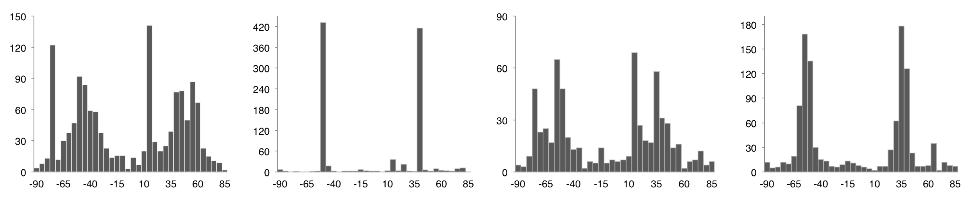
The urban form refers to the physical layout of the city: It is set by the distribution of urban elements, such as streets, blocks, plots, and buildings. There are different types or urban forms: grid or orthogonal, linear, radial, and irregular. Representative samples of the urban form for each one of the districts are shown in Figure 2, where plans are drawn at the same scale, blocks are shown in black, streets are in white, and pedestrian streets are in light brown. Ciutat Vella exhibits an organic and irregular structure—distinctive of the Middle Ages—Eixample is a planned grid structure, Les Corts recalls a radial plan, and Gràcia is based on an orthogonal structure of different size plots. Hence, a fine-grain urban fabric characterizes Ciutat Vella and Gràcia and a coarse-grain urban fabric distinguishes Eixample and Les Corts. Based on previous measurements of the urban street networks [57,58,59,60,61,62], we compute Shannon’s entropy of the urban structure to provide quantitative information that is useful in the diversity analysis. In this methodology, the street orientation, length of the built tract of the street, and height of the adjacent buildings are measured in the four districts’ area. Then, the values for each variable and district are arranged—by absolute frequencies—in fixed bins $j=1,\dots ,m$: Histograms illustrate this distribution (e.g., histograms for streets’ orientation in Figure 3). Once the measures are binned, Shannon’s entropy $S_i$ is computed for each ith distribution (e.g., the streets’ orientation in a district) following $S_i=-\kappa {\sum }_{j=1}^m{p}_{ij}ln\left(p_{ij}\right)$ for $i=1,2,\dots ,n$. $\kappa$ represents a positive constant, and $p_{ij}$ is the probability of the variable falling in the jth bin. When the probability is zero, $p_{ij}=0$, the supposition $p_{ij}ln\left(p_{ij}\right)=0$ is implemented. Entropy values for each one of the ith variables and districts are shown in

Table 1. Urban structure’s metrics using Shannon’s entropy.

Metric	Ciutat Vella	Eixample	Les Corts	Gràcia
Streets’ lenght	2.963	2.910	3.746	3.345
Streets’ orientation	4.648	2.156	4.615	4.046
Buildings height	2.905	3.137	3.398	3.207
Average entropy	3.506	2.734	3.920	3.533

. This information entropy metric reveals the degree of order of the urban structure: The low entropy exhibited by Eixample corresponds to its grid structure with a high degree of order. Les Corts and Ciutat Vella, on the other hand, present a high entropy that displays their heterogeneous urban structure, with neighborhoods having a dissimilar urban layout not only in formal aspects but also in the size of their entities (streets, plots, blocks, and empty urban spaces, etc.).

Regarding the socioeconomic component, we consider characteristics such as employment rate, income, education, population age, and percentage of foreigners (see

Table 2. Case study demographic description.

City/District	Population		Surface	Pop. Density	Foreigners
			km${}^2$	(inhab/km${}^2$)	Population	Of District	Of City
Ciutat Vella	101,387	6%	4.37	23,201	45,357	45%	16%
Eixample	266,416	16%	7.48	35,617	53,393	20%	19%
Les Corts	82,033	5%	6.02	13,627	9796	12%	3%
Gràcia	121,347	7%	4.19	28,961	19,574	16%	7%
Barcelona	1,620,809	100%	102.16	15,865	284,907	18%	100%

Data for 2017 from the Index Statistical yearbooks of Barcelona [56].

for relevant demographic data of the case study, including percentages for each district with respect to the city). The district of Ciutat Vella is the oldest one, constituting itself the historical city center. The district of Eixample was designed by Ildefons Cerdà in 1859 as part of the widely known urbanism plan called “Plan Cerdà” [63,64,65]. Eixample district is also the densest district of Barcelona with a population density of 35,617 inhabitants per km${}^2$. In the case of the districts of Les Corts and Gràcia, those were former independent municipalities annexed to the city in the last decade of the 19th century after a major conurbation process. As commented before, we select these districts to be representative and to constitute the urban essence of Barcelona.

2.2. Multivariate Description of the Case Study

The urban system description of the case study is achieved through a multivariate dataset that incorporates measurements of environmental and socioeconomic variables from the years 2003 to 2015. This dataset is a matrix containing 40 indicators (variables) and 52 individuals: Each individual represents a district in a given year (e.g., “CiutatVella 2003”, “Ciutat Vella 2004”, “Eixample 2003”, etc.). To construct the multivariate description of the case study, we considered the availability of time-dependent disaggregated data in the case of the four districts. Our dataset collects the information in the open databases of Departament d’Estadística [56] and Agencia de Salut Pública de Barcelona [66], and it is shown in

Table 3. Dataset for the district of Ciutat Vella between 2003 and 2015.

Type		Id	Indicators	Unit	2003	2004	2005	2006	2007	2008	2009	2010	2011	2012	2013	2014	2015
INPUT	Supportive	A1	Residential area	m${}^2$/person	37.0	36.7	35.5	34.9	35.5	35.4	36.9	37.9	38.2	38.0	38.4	39.3	39.5
		A2	Commercial area	m${}^2$/person	5.6	5.6	5.4	5.4	5.5	5.6	5.9	6.1	6.2	6.2	6.3	6.5	6.5
		A3	Office buildings	m${}^2$/person	6.6	6.6	6.4	6.3	6.4	6.4	6.6	7.1	7.0	6.9	7.2	7.5	7.4
		A4	Educational buildings	m${}^2$/person	3.0	3.0	2.9	2.9	3.0	3.0	3.2	3.3	3.4	3.5	3.5	3.6	3.7
		A5	Health service buildings	m${}^2$/person	0.6	0.6	0.6	0.6	0.6	0.6	0.6	0.6	0.6	0.6	0.7	0.7	0.7
		A6	Sport area	m${}^2$/person	0.3	0.3	0.3	0.3	0.3	0.3	0.3	0.3	0.4	0.4	0.4	0.4	0.4
		A7	Religious buildings	m${}^2$/person	0.8	0.8	0.8	0.7	0.7	0.7	0.8	0.8	0.8	0.8	0.8	0.8	0.8
		A8	Entertainment buildings	m${}^2$/person	0.8	0.8	0.8	0.7	0.7	0.7	0.8	0.8	0.8	0.7	0.8	0.8	0.8
		A9	Other land uses	m${}^2$/person	2.5	2.5	2.5	2.4	2.5	2.5	2.6	2.8	2.9	2.7	2.7	2.8	2.8
		A10	Cultural centres	unit/person ($\times {10}^{-4}$)	2.6	2.0	2.2	2.2	2.1	2.1	2.4	2.8	2.7	2.6	2.6	2.8	2.8
		A11	Sport centres	unit/person ($\times {10}^{-3}$)	1.1	1.1	1.0	1.1	1.1	1.1	1.4	1.5	1.4	1.4	1.5	1.7	1.7
		A12	Security level in the neighbourhood	Points	4.8	4.7	4.9	5.0	5.3	5.2	4.9	4.9	4.8	5.2	5.2	5.4	5.2
		A13	Public water fountains	unit/person ($\times {10}^{-4}$)	9.9	9.6	9.2	9.1	9.0	9.1	9.4	9.6	9.8	9.6	9.5	9.4	10.1
		A14	Playgrounds	unit/person ($\times {10}^{-4}$)	2.1	2.0	1.8	1.9	2.2	2.4	2.4	2.8	2.7	2.8	3.1	3.2	3.2
		A15	Active market stalls	unit/person ($\times {10}^{-3}$)	9.8	9.5	8.7	8.6	8.6	8.5	8.8	9.1	9.2	9.1	9.2	9.4	9.4
		A16	Street trees (Unit = 5.6 m${}^2$)	unit/person ($\times {10}^{-2}$)	6.4	6.3	5.8	5.8	6.0	5.8	6.5	6.5	6.7	6.8	6.7	6.9	6.9
		A17	Urban parks	ha/person ($\times {10}^{-4}$)	3.5	3.5	3.3	3.3	3.3	3.3	3.5	3.6	3.6	3.6	3.6	3.7	3.7
		A18	Urban green area besides parks	ha/person ($\times {10}^{-4}$)	2.4	2.4	2.3	2.2	2.3	2.3	2.4	2.5	2.5	2.5	2.5	2.5	2.5
OUTPUT	Pressure	B1	Natural growth rate	-	-4.7	-1.5	-1.2	-1.1	-1.4	0.1	0.4	0	0.9	-0.3	-0.5	-0.5	-0.3
		B2	Population density	people/ha	244	246	254	258	255	255	245	239	236	239	237	231	229
		B3	Total number of motor vehicles	unit/person	0.4	0.4	0.4	0.4	0.4	0.4	0.5	0.5	0.5	0.5	0.4	0.4	0.4
		B4	Total volume of water supplied to the commerce	m${}^3$/person	36.3	35.6	34.0	32.7	34.2	32.7	32.7	33.5	33.8	33.1	33.5	9.6	9.7
		B5	Total volume of water supplied to domestic consumption	m${}^3$/person	41.7	40.8	39.0	37.7	38.1	37.1	38.1	38.7	38.9	37.9	37.1	37.6	38.0
		B6	Total volume of water supplied to the industry	m${}^3$/person	5.3	5.0	4.6	4.4	4.3	3.6	3.4	3.3	4.2	3.0	2.7	26.6	27.5
		B7	Total volume of water supplied to other usages	m${}^3$/person	10.6	10.3	9.7	10.8	10.0	7.0	8.4	8.6	9.1	9.5	9.3	9.8	12.6
		B8	Available household income per capita	Index	71.0	70.8	72.0	72.6	73.5	71.2	74.2	75.2	76.4	76.6	77.2	79.7	85.5
		B9	Accommodation places	unit/person ($\times {10}^{-1}$)	1.1	1.2	1.2	1.2	1.2	1.3	1.6	1.8	1.9	1.9	1.9	2.0	2.1
		B10	Final energy consumption	MWh/year.person	2.9	3.1	3.2	2.9	2.8	2.9	3.1	3.3	2.9	3.1	2.9	3.2	3.2
		B11	Parking area	m${}^2$/person	3.2	3.3	3.3	3.4	3.6	3.7	3.9	4.4	4.5	4.5	4.6	4.8	4.8
		B12	Industrial area	m${}^2$/person	5.1	5.0	4.7	4.5	4.5	4.4	4.5	4.5	4.5	4.3	4.3	4.4	4.4
DEST-	RUCTIVE	C1	Average levels of PM${}_{10}$	$\mathsf{\mu }$g/m${}^3$	51	46	47	52	43	43	33	29	31.6	31	26	27	31
		C2	Average levels of NO${}_2$	$\mathsf{\mu }$g/m${}^3$	57	43	48	47	46	42	46	46	40	42	35	37	42
		C3	Average levels of CO	mg/m${}^3$	0.5	0.5	0.5	0.3	0.4	0.3	0.4	0.4	0.3	0.3	0.3	0.3	0.3
		C4	Collected volume of non-recyclable waste	ton/person ($\times {10}^{-1}$)	2.4	2.2	2.1	2.1	2.2	2.0	2.0	2.2	2.2	1.9	1.9	2.0	2.0
		C5	Traffic accidents	unit/person ($\times {10}^{-3}$)	7.8	7.0	6.8	6.2	6.9	6.0	5.9	5.3	5.5	5.5	5.5	5.3	5.9
REGENE-	RATIVE	D1	Collected volume of paper and cardboard	ton/person ($\times {10}^{-2}$)	2.2	2.5	2.9	3.0	3.4	3.5	3.2	3.9	2.9	2.4	2.1	2.3	2.3
		D2	Collected volume of glass	ton/person ($\times {10}^{-3}$)	8.0	8.4	8.8	9.1	10.8	11.4	12.1	15.1	14.9	14.1	14.2	15.1	15.0
		D3	Collected volume of containers	ton/person ($\times {10}^{-3}$)	4.2	4.5	4.7	4.9	6.1	6.6	7.0	9.4	9.0	8.3	8.0	8.4	8.4
		D4	Maintenance cost	Miles of /person ($\times {10}^{-3}$)	6.9	6.8	5.6	6.9	7.2	7.4	7.8	8.3	8.4	8.1	8.2	8.4	8.4
		D5	Streets and zones with pedestrian priority	ha/person ($\times {10}^{-4}$)	2.0	2.1	2.0	1.9	2.0	1.9	2.1	2.2	2.3	2.3	2.3	2.7	2.8

for the district of Ciutat Vella between 2003 and 2015. The datasets for the remaining districts (Eixample, Les Corts, and Gràcia) are presented in Appendices Appendix A, Appendix B and Appendix C. This particular time-span—from 2003 to 2015—has been chosen regarding the data availability at the district scale: Before 2003, only a few indicators were reported at this scale.

Most of the variables have been measured on a per capita basis in order to neutralize the effect of districts’ population size. This fact allows us to make a comparison focused on services and consumptions for each inhabitant of a given district. However, the discussion on analyzing urban systems based on aggregated or disaggregated data, normalized either by surface or population, remains an open debate. Particularly, we consider raw values for general or disaggregated indicators: Security level in the neighborhood (A12), Natural growth rate (B1), Population density (B2), Available household income per capita (B8), Average levels of PM${}_{10}$ (C1), Average levels of NO${}_2$ (C2), and Average values of CO (C3).

Within the framework of urban ecology, we use the concept of urban metabolism in order to describe and classify the interactions between the different components that take place in the city. One of the main ideas of this methodology is to integrate social, environmental, and economic variables into categories that characterize the ecological structure, diversity of amenities, population pressures, and consumption of the urban system: It is intended to portray the flows of matter, information, and energy in an ecosystem. We arrange our system of variables based on some previous indexes developed within the frameworks of urban metabolism and urban sustainability [67,68,69,70], but we include some additional variables that characterize social interactions, diversity of land uses, and liveability. Following Zhang et al. [67], we group the variables (presented in Table 3) into four metabolic categories:

• Input Supportive. This category comprises 18 indicators and portrays the natural capital of the city and the liveability and the complexity of urban services. Some indicators in this category describe the diversity of economic activities and institutions associated with each district. We refer to the land use areas and buildings: housing, commerce, offices, education, health services, sport, religion, and entertainment, among others.
• Output Pressure. It includes 12 indicators that describe the pressure exerted by the economic and social subsystems over the natural subsystem. This category is mostly related to the population size (social subsystem) and its consumption demand.
• Destructive Metabolism. It includes 5 indicators that reveal the environmental pollution within the urban system, particularly described by air pollution and waste generation indicators. We also include the number of traffic accidents in order to measure one particular aspect of the non-liveability character of an urban system.
• Regenerative Metabolism. It comprises 5 indicators related to ecological construction upon regenerative infrastructure and environmental care.

2.3. Multivariate Statistical Analysis of the Dataset

Since there is a large amount of information comprised in the multivariate dataset, its examination is complicated; thus, statistical methods are implemented to ease the analysis of the urban system. In the first place, we display in Figure 4 the correlation matrix among the 40 variables (that has been produced in R [71] using the corrplot package [72]), which is colored according to the correlation coefficient. We realize that the interactions that take place in the city between districts and indicators are far too complex, and therefore, the dimensionality reduction given by the PCA is justified. Specifically, we rely on this mathematical procedure to transform the original $x$—dimensional dataset space into a reduced $y$—dimensional component space—being the cardinality of y lesser or equal than x—by solving the eigenvalues problem [55]. For the sake of concision, we omit the mathematical formulation of the eigenvalues problem of the correlation matrix (see Jolliffe [34] for a thorough explanation on this topic). Here, we are mainly interested in the transformation given by the solution of the eigenvalue problem.

The PCA transformation leads to the description of the original dataset by means of a set of linearly independent variables, which are the so-called principal component [34,73]. The principal components are uncorrelated and ordered so that the first component describes most of the variance of the dataset, and each successive component describes the largest possible variance after the previous components [34]. Therefore, if only the subset of the first y principal components is selected, $y<<x$, the dimensionality can be reduced whilst a great percentage of the variance of the original correlation matrix is maintained. The main advantage of PCA lies in its ability to reduce the dimensionality of the multivariate system while extracting its main characteristics in the dimensionally reduced description. In the case study, we reduce the 40-dimension description to only 3 dimensions per individual. The PCA calculation is conducted in R Software [71] using the FactoMineR package [74]; the results are displayed using the ggplot2 [75] and factoextra [76] packages.

Since the variables are measured in different units and the measurements for each variable can vary up to two orders of magnitude, we perform a scaling of the raw data matrix prior to the application of the PCA. The data preparation is intended to make comparable data of different units and scales such that the standardized data is scaled to have standard deviation one and mean zero.

In order to visualize the outcome of the analysis, we display the relationship among the variables (indicators) and individuals (districts) using covariance biplots [34,77,78]. In biplots, we make profit of the new low-dimensionality of the system by plotting individuals and variables against the three selected principal components, which are placed at the axes of the plots [77]. Using biplots and loadings (

Table 4. Component loadings (correlations between variables and components) for the three principal components. Values above the 0.4 threshold are highlighted in boldface font.

Type		Id	Indicators	PC1	PC2	PC3
INPUT	Supportive	A1	Residential area	0.88	−0.23	0.23
		A2	Commercial area	0.16	0.11	0.91
		A3	Office buildings	0.17	0.33	0.90
		A4	Educational buildings	0.24	0.95	0.10
		A5	Health service buildings	0.54	−0.23	−0.66
		A6	Sport area	0.53	0.82	−0.10
		A7	Religious buildings	−0.82	0.31	−0.39
		A8	Entertainment buildings	−0.86	−0.12	0.46
		A9	Other land uses	−0.65	0.65	0.38
		A10	Cultural centres	−0.95	−0.01	0.23
		A11	Sport centres	−0.72	0.46	−0.37
		A12	Security level in the neighbourhood	0.89	−0.01	−0.40
		A13	Public water fountains	−0.69	0.52	−0.35
		A14	Playgrounds	0.51	0.81	−0.13
		A15	Active market stalls	−0.96	−0.22	0.00
		A16	Street trees (Unit = 5.6 m${}^2$)	0.62	0.75	0.15
		A17	Urban parks	−0.50	0.83	−0.07
		A18	Urban green area besides parks	0.34	0.92	0.00
OUTPUT	Pressure	B1	Natural growth rate	−0.47	0.42	−0.38
		B2	Population density	−0.05	−0.95	0.15
		B3	Total number of motor vehicles	0.93	0.33	−0.04
		B4	Total volume of water supplied to the commerce	−0.29	−0.16	0.92
		B5	Total volume of water supplied to domestic consumption	0.70	−0.19	0.26
		B6	Total volume of water supplied to the industry	−0.28	0.78	0.51
		B7	Total volume of water supplied to other usages	−0.74	0.44	0.24
		B8	Available household income per capita	0.93	0.33	−0.05
		B9	Accommodation places	−0.66	0.47	0.50
		B10	Final energy consumption	0.86	−0.04	0.27
		B11	Parking area	0.81	0.57	0.00
		B12	Industrial area	0.63	0.20	0.72
DESTRUC-	TIVE	C1	Average levels of PM${}_{10}$	−0.08	−0.62	0.25
		C2	Average levels of NO${}_2$	0.16	−0.88	−0.17
		C3	Average levels of CO	0.34	−0.81	0.19
		C4	Collected volume of non−recyclable waste	0.91	−0.21	0.08
		C5	Traffic accidents	0.54	−0.11	0.81
REGENE-	RATIVE	D1	Collected volume of paper and cardboard	0.62	0.35	0.00
		D2	Collected volume of glass	0.73	0.55	−0.17
		D3	Collected volume of containers	0.68	0.56	−0.18
		D4	Maintenance cost	−0.51	0.82	−0.14
		D5	Streets and zones with pedestrian priority	−0.95	0.19	0.18

), we identify correlations (direct, inverse, or null) between variables and principal components such that a conceptual meaning is given to each principal component in a process that we call “labelling”. Individuals can be analyzed in their relative positions to the labeled principal components. This will be further exemplified in the next sections.

Also, distance measures can be used to quantify the differences—dissimilarities—between individuals. We perform some statistics of the districts’ performance, where districts’ positions are accounted as events: Each district’s location is accounted as a single observation such that the average value of the districts’ positions—or centroids—can be used as a representative location. We propose to calculate the component-wise and Euclidean distances between districts’ centroids in order to quantify diversity. Thus, the next step of analyzing diversity fostering resilience can be done based on quantitative results.

Furthermore, we implement MFA [46] for summarizing and visualizing urban metabolism categories and their relation with the principal components’ description of districts. Particularly, MFA is an extension of PCA that takes advantage of the categorical groups of variables by weighting—or balancing—the contribution of the variables in each group [48]. Conclusions on the metabolism of the city can be addressed by understanding the contribution of variables in each urban metabolism category to the principal component’s description of districts and, hence, of the city.

3. Results

In this section, we present the results of applying the multivariate statistical methodology to our case study. The results are presented in the following order: firstly, the dimensionality reduction given by the PCA application, the description of each district as given by the PCA, and the variables’ loadings for each principal component. Secondly, we explain the labeling of the selected principal components. Lastly, the MFA results of the urban metabolism categories.

3.1. Principal Component Analysis

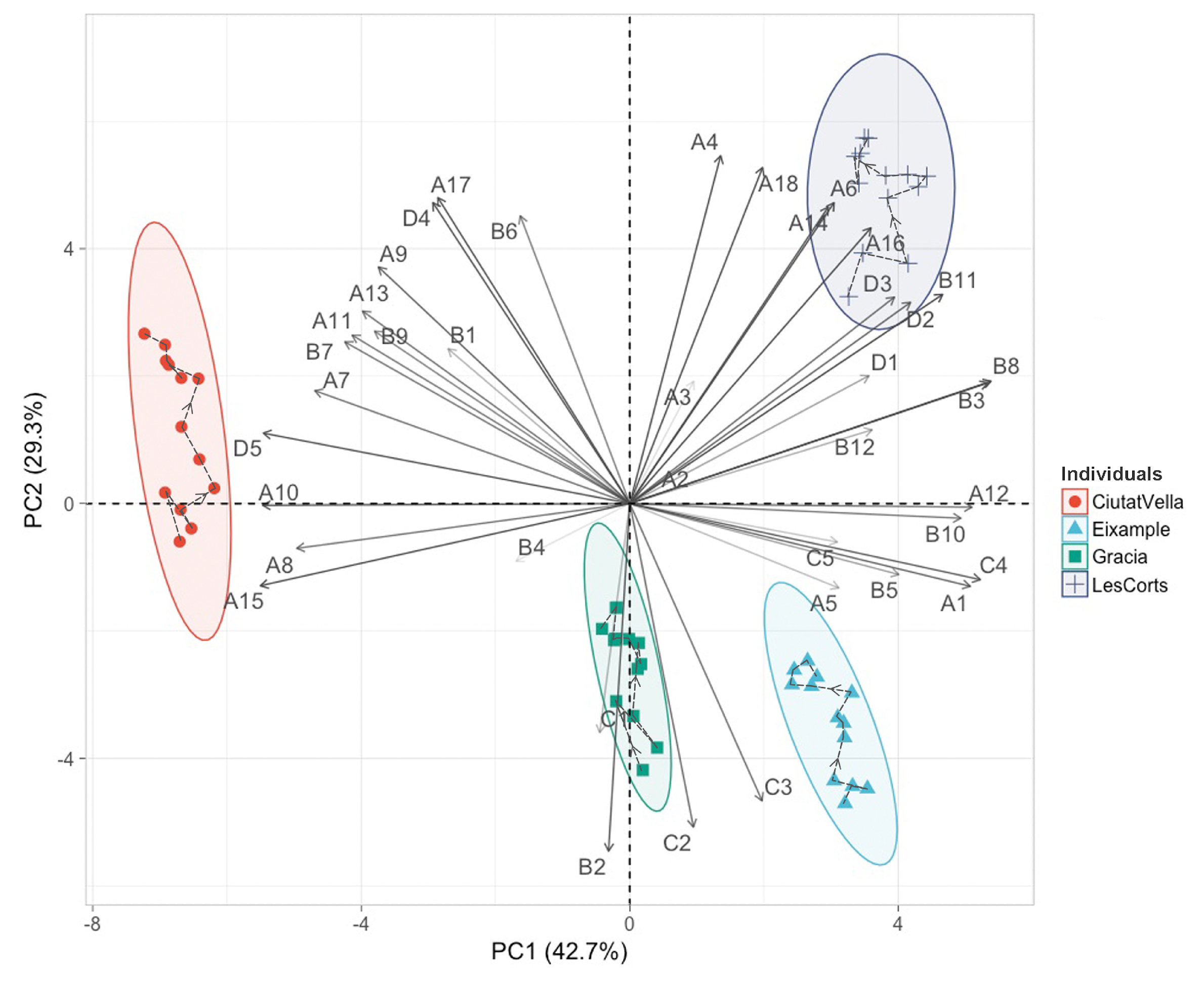
As described in the methodology, we use R Software [71] and the FactoMineR package [74] to perform the standardized PCA. Since FactoMineR uses a singular value decomposition algorithm, the PCA is calculated over the standardized correlation matrix, where a matrix of 40 uncorrelated components is obtained.

Table 5. Decomposition of variance per component of the Principal Component Analysis (PCA).

Component	Eigenvalue	Percentage of Variance	Cumulative Percentage of Variance
1	17.07	42.69	42.69
2	11.70	29.25	71.94
3	6.31	15.78	87.73
4	2.14	5.36	93.10
5	0.82	2.05	95.15
6	0.48	1.20	96.36
7	0.35	0.87	97.24
8	0.27	0.68	97.92
9	0.19	0.48	98.40
10	0.14	0.37	98.78

shows the percentage of variance and the eigenvalues for the first 10 components of this matrix. The remaining components (30) correspond to a residual amount of variance. By selecting only the first three principal components, we reduce the dimensionality of the multivariate description so that the graphical representation and its subsequent interpretation are simplified. The first three principal components describe 87.7% of the total variance: The first component describes 42.7% of the variance, the second one describes 29.3% of the variance, and the third component describes 15.8% of the variance. In the case of the goodness of fit, we rely on the following metrics to verify the choice of the three first components: the Root Mean Square of the Residuals (RMSR) is 0.05, and the fit based upon off-diagonal values is 0.99. We label these three principal components as “Social Background” (PC1), “Ecological Background” (PC2), and “Urban morphology and architectural typology” (PC3) according to the urban description that they make (to be explained next).

Correlations between indicators and principal components are described by the components’ loadings. Table 4 shows the positive, negative, and null loads for each one of the three principal components. A high absolute load indicates an important contribution of that variable to the percentage of variation covered by that particular component. Its sign implies a direct (+) or an inverse (−) correlation.

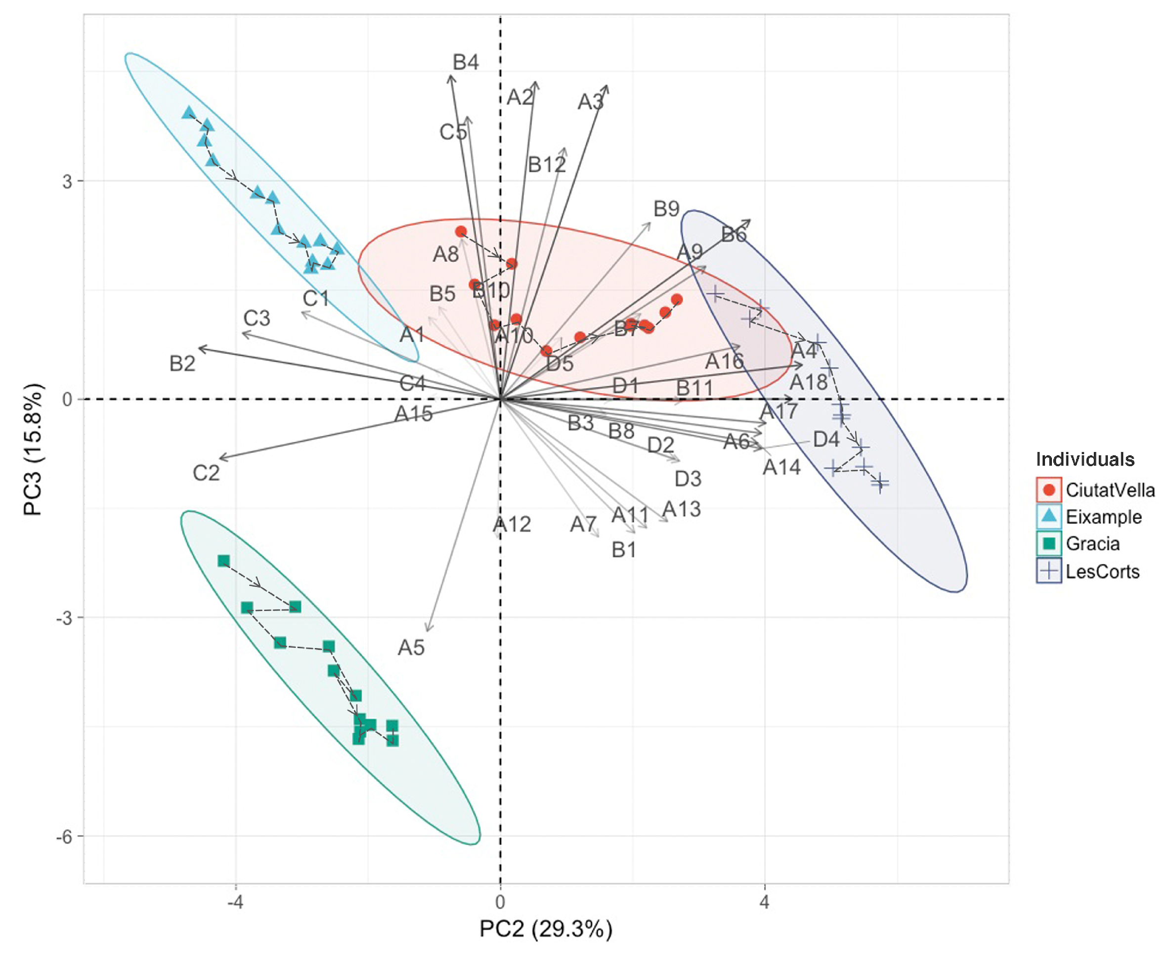
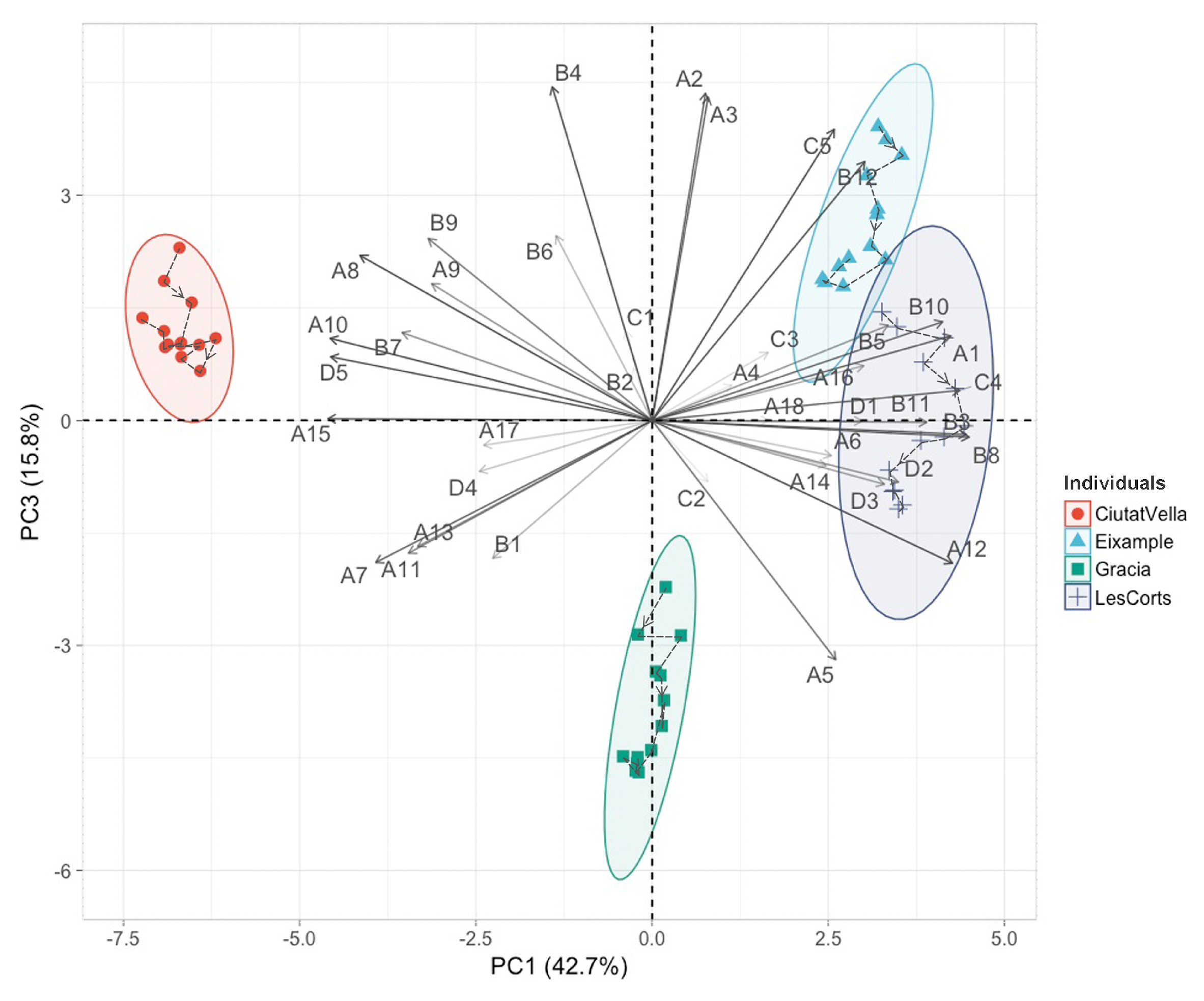
Figure 5, Figure 6 and Figure 7 show two-dimensional biplots, each one showing the combination of two of the three principal components. Points (individuals) represent the districts in each year of the time period under analysis. Individuals are shown with a specific color and shape for each district. The temporal evolution of districts is depicted with dashed arrows connecting the different coordinates from the year 2003 to the year 2015.

Averaged positions are presented in

Table 6. District’s centroids.

District	Notation	PC1	PC2	PC3
Ciutat Vella	$\overline{C}$	−6.705	1.133	1.227
Eixample	$\overline{E}$	2.993	−3.457	2.632
Gràcia	$\overline{G}$	−0.03	−2.569	−3.828
Les Corts	$\overline{L}$	3.743	4.893	−0.031

with the notation for each district. We also calculate the district’s displacement from the initial to the final year of the time span. This calculation is given in

Table 7. Displacements of districts in the principal components.

District	PC1	PC2	PC3
Ciutat Vella	−0.526	3.263	−0.933
Eixample	−0.417	1.985	−1.752
Gràcia	−0.401	2.547	−2.266
Les Corts	0.233	2.492	−2.627

for each principal component, and it is useful to describe the district’s variation related to the principal component. Finally, in

Table 8. Component-wise distances between districts’ centroids.

PC1					PC2					PC3
	$\overline{C}$	$\overline{E}$	$\overline{G}$	$\overline{L}$		$\overline{C}$	$\overline{E}$	$\overline{G}$	$\overline{L}$		$\overline{C}$	$\overline{E}$	$\overline{G}$	$\overline{L}$
$\overline{C}$	0	9.698	6.675	10.448	$\overline{C}$	0	4.59	3.702	3.761	$\overline{C}$	0	1.405	5.055	1.257
$\overline{E}$	9.698	0	3.023	0.75	$\overline{E}$	4.59	0	0.888	8.351	$\overline{E}$	1.405	0	6.461	2.663
$\overline{G}$	6.675	3.023	0	3.773	$\overline{G}$	3.702	0.888	0	7.462	$\overline{G}$	5.055	6.461	0	3.798
$\overline{L}$	10.448	0.75	3.773	0	$\overline{L}$	3.761	8.351	7.462	0	$\overline{L}$	1.257	2.663	3.798	0

and

Table 9. Euclidean distances between districts’ centroids.

	$\overline{\mathit{C}}$	$\overline{\mathit{E}}$	$\overline{\mathit{G}}$	$\overline{\mathit{L}}$
$\overline{C}$	0	10.821	9.155	11.175
$\overline{E}$	10.821	0	7.188	8.797
$\overline{G}$	9.155	7.188	0	9.184
$\overline{L}$	11.175	8.797	9.184	0

, we present the component-wise and Euclidean distances between districts’ centroids, respectively.

3.2. Labeling the Principal Components

Vectors in biplots of Figure 5, Figure 6 and Figure 7 portray the correlations of the different variables with the principal components: The vector length represents the influence—or loading—of the variable into that component. In order to give a conceptual label to each principal component, we select some of the variables that have large loadings in the component. Then, we identify the type of correlation between the highlighted variables (direct or inverse) and classify the variables showing no relation with the component. A conceptual meaning is given to each component by recognizing the type of variables that characterizes it. Each labeling of the principal components is detailed next.

3.2.1. First Principal Component PC1—“Social Background”

As presented in Table 5, the First Principal Component (PC1) explains 42.7% of the total variance. It can be observed in Figure 5 and Figure 7 and in Table 4 that the variables with higher loadings on this component are, among others, A1, A7, A8, A10, A11, A12, A14, A15, A16, B3, B7, B8, B11, B12, C4, D1, D2, D3, and D5. The positively correlated variables are related to available income, the number of vehicles, and housing. Instead, the negatively correlated variables are related to urban amenities such as market stalls; pedestrian zones; and cultural, religious, and sports centers. This component is, therefore, displaying the diversity of land uses and confronts two different types of neighborhoods: on the one side, housing and predominant car-usage zones, and on the other, diverse and pedestrian zones. It also reveals the social interactions that take place in the city, which are directly related to diversity and, thus, with economic development, productivity, and innovation [5,6]. We also observe that the variables that are not represented by this component are population density, commercial areas, offices, and average levels of PM${}_{10}$ and NO${}_2$. Hence, we label this component as “Social background”.

3.2.2. Second Principal Component (PC2)—“Ecological Background”

In the case of PC2, it accounts for 29.3% of the total variance. As shown in Figure 5 and Figure 6 and in Table 4 variables with noteworthy loadings on this component are related to air pollution, population density, street trees, urban parks, and green areas. Moreover, there are some variables that are not described by this component at all, such as the number of cultural centers, security level, and energy consumption. Consequently, it is related to the ecological structure of each district, and we label this component as “Ecological Background”.

3.2.3. Third Principal Component (PC3)—“Urban form and Architectural Typology”

PC3 explains 15.8% of the total variance. We observe in Figure 6 and Figure 7 and in Table 5 that variables with high loadings on this component are related to commercial, corporative, and industrial areas, as well as to traffic accidents. There are some variables, such as green areas, collected paper and cardboard, market stalls, and parking areas that are not described by this component. Although the indicators related to this principal component are describing large-surface activities such as commerce, offices, and industries, we label it on the fact that it also suggests a distinctive neighbourhood character, with a particular urban form and architectural typology. Consequently, we label this component as “Urban and architectural typology”.

3.3. Multiple Factor Analysis

We complement the PCA description by reading the contribution of the variables in each of the four metabolic categories. In addition to the districts’ coordinates (Figure 5, Figure 6 and Figure 7), new relations arise between metabolic types of variables when those categories are described using the principal components. In particular,

Table 10. Multiple Factor Analysis (MFA) results for the groups of variables.

Metabolism Categories (Groups)	Coordinates			Contribution (%)
	PC1	PC2	PC3	PC1	PC2	PC3
Input	0.95	0.66	0.38	29.12	27.77	34.49
Output	0.97	0.48	0.42	29.87	20.05	38.07
Destructive	0.51	0.70	0.27	15.72	29.58	24.37
Regenerative	0.82	0.53	0.03	25.19	22.58	3.05

shows the relation between groups and principal components; each group of variables—a metabolism type—contributes to the construction of the principal components. As shown in that table, output pressure and input supportive types of variables contribute the most to the construction of the first component (29.9% and 29.2%, respectively); the minor contribution, in this case, is from the destructive metabolism type of variables (15.7%). Instead, the four groups of variables are very close together in the second component; only the destructive metabolism category has a differentiated contribution in this component with 29.6%. Regarding the third component, it is related to both output pressure and input supportive types of variables—of which the contributions are 38.1%, and 34.5%, respectively—but it is not linked with the regenerative metabolism category (contributing only 3.0%). These facts suggest that the output pressure and the input supportive groups of variables are defining the first and third components, and in the case of the second component, although all metabolism groups contribute similarly, the destructive metabolism group mostly characterizes it.

4. Discussion

Now, we interpret the comprised information in the dimensionally reduced description by considering the districts’ performance. Since the principal components have been labeled, in the first part of this section, we read the description of each district: Urban diversity can be recognized and quantified using the results of the previous section. Then, we evaluate the metabolic performance of districts by correlating individuals, principal components, and metabolic groups of variables, as given by the MFA results. We further discuss the link between urban diversity and resilience. Finally, we analyze the time-dependent evolution of the districts and the possible increase—or decrease—of urban diversity.

4.1. Urban Diversity

We follow the previous studies in References [79,80,81,82,83,84], which have taken advantage of biplot graphs to display diversity in multiple systems. Using the PCA representation (i.e., biplots), we perform a descriptive analysis of diversity with respect to principal components. To achieve this reading, we determine each district’s performance [78] (positions in biplots of Figure 5, Figure 6 and Figure 7) and quantify diversity as the Euclidean distance [85] between districts’ centroids.

The first notable characteristic of the districts’ performance in the PC1-Social Background is that this component separates the districts of Ciutat Vella and Les Corts roughly by 10.5 units of distance (see Table 8), one unit more than the distance between Ciutat Vella and Eixample (9.7), and four units more than distance between Ciutat Vella and Gràcia (6.7). The districts of Eixample and Les Corts are closely together (i.e., the distance between them is of 0.75), and relatively near to Gràcia (being 3.0 units apart from Eixample and 3.8 from Les Corts). Certainly, differentiated social interactions for Ciutat Vella are identifiable from the raw data: This district owns community amenities for the whole city, and in this sense, it exhibits high loads on the indicators related to religious and entertainment buildings, exclusive pedestrian areas, market stalls, and cultural and sport centers, among others. This can be explained because, in the last decade, an intensive culture-based program of urban regeneration has been developed in the district—mainly in The Raval, one of the neighborhoods of Ciutat Vella—in order to face urban marginality and social stigmatization, constituting itself a center for culture and creativity [86]. On the other hand, Les Corts—and Eixample, to a lesser extent—are mainly residential districts, which are characterized, among other features, by higher income, higher security level, a large number of vehicles, and large parking areas. Therefore, PCA results agree with the actual nature of the districts, where districts are differentiated by the quantity and quality of social interactions associated with the diversity of land uses and functional typologies.

Figure 6 offers a remarkable characteristic, it clearly shows the emergence of “two Barcelonas”, with PC2-Ecological Background drawing a division between two groups of districts: Eixample and Gràcia on one hand (Figure 6, left) and Les Corts on the other (Figure 6, right), with an average distance of eight units between them. Les Corts has a good performance in the indicators related to the quality of public spaces and with green and recreational areas. Particularly, this district is defined by the following indicators: urban parks (A17), urban green areas (A18), educational buildings (A4), sports area (A6), playgrounds (A14), and street trees (A16). We observe that these indicators are inversely correlated with air pollution indicators (see Figure 4). In contrast, the group of districts concerning Eixample and Gràcia is described mainly by the average levels of PM${}_{10}$, NO${}_2$, and CO. Therefore, Eixample and Gràcia exhibit a great flow of pollutants—compared to all the districts of the city—is linked to high population density (B2), and lacks green and recreational spaces (see the correlation in Figure 4). According to Barcelona City Council [87], the road transport activity in 2013 was responsible for 67.6% and 68.9% of the NO${}_2$ emissions in Eixample and Gràcia, respectively. Furthermore, because of its high traffic, Eixample experiences the highest noise levels (over 70 dB(A)) in the city [88]. In order to improve the environmental quality of these districts and to move forward to positive performances in PC2-Ecological Background, some planning strategies should be applied. Since the compact form and the mixed use development of these districts encourages walkability [89], actions should focus on reducing road activity and on promoting cycling. Moreover, taking into account the high density of these districts and the scarcity of green areas, green roofs, and green walls represents some alternative solutions.

Regarding PC3-Urban Form and Architectural Typology, this principal component segregates Eixample and Gràcia (see Figure 6 and Figure 7), with a gap of around seven units of distance (6.5). This can be explained since Eixample is mainly associated with a larger amount of offices and greater commercial and industrial areas than those in Gràcia. In fact, Gràcia has the lowest records in these indicators for the whole case study. On the one side, Eixample displays a metropolitan scale due to its size, compactness, high density, and proximity to the city center (see Figure 1). Eixample, being designed in 1859, has a compact urban form (see Figure 2) consisting of a strict grid pattern with large straight streets, square blocks with chamfered corners (133 m side), and wide crossing avenues [63,64,65]. In terms of architectural typology, Eixample is characterized by large-surface and high-rise buildings (up to 7 floors) compared with the average height of buildings in Barcelona. Hence, it allows a mixed-used development. Gràcia, on the other hand, is more related to a human scale of interactions since it was originally an independent and smaller town. This district was established originally in 1626 as a village—out of Barcelona’s boundaries—and displays a distinct urban layout: It has an orthogonal grid, with small and medium size blocks, crossed by narrow streets (see Figure 2 and Figure 3, and Table 1). It is defined by low and medium-rise buildings of medium-size plots.

The indicator of traffic accidents also unveils the urban form and the amount and scale of interactions: Because of its straight streets, Eixample’s urban layout encourages car mobility with higher levels of street traffic and higher car speeds [88]; hence, traffic accidents are more frequent. Instead, the human scale and car-restricted streets of Gràcia possess lower traffic and consequently less road and car accidents. In summary, both districts exhibit differentiated neighborhood characters and scales which are captured in the multivariate analysis.

The PCA applied on the multivariate system description reveals correlations among indicators and districts, which are difficult to identify only with the raw data (as it that has been shown in Figure 4 or with the urban structure metrics in Table 1), and allows us to understand the city at a macro level. It exhibits distinctive attributes of the four districts of the case study, as demonstrated by each one of the principal component descriptions presented before. In the case of the first component, it exposes an “inner diversity” of land uses, contrasting Ciutat Vella and Les Corts that own different functional typologies and are the most distant or are the most different of the case study. Our findings portray the different types of “Barcelonas” and, thus, the re-evaluation of the a priori homogeneity of the city. This is more evident when looking at the second principal component; the description made by this component draws a clear division between two distinguishable groups or types of districts: Les Corts on one side, characterized by large public spaces and green and recreational areas, and Eixample and Gràcia on the other, identified as dense and highly polluted.

Moreover, the measurement of the relative distances between the districts as described by PCA gives the main instrument for quantifying diversity at the city scale. The Euclidean distance among districts (i.e., three-dimensional distance between districts’ centroids) determine that Ciutat Vella and Les Corts are the most distant—different—districts of the case study, with an average distance of 11.17 units; Ciutat Vella is also widely separated—10.82 units—from Eixample; and Eixample and Gràcia are the closest—similar—ones, with an average distance among them of 7.19 units (as presented in Table 9). These distances in a non-diverse case study would give close to zero values and imply districts’ stacks in specific locations. This has not been the case of the present results, in which significant distances among the districts indicate a diverse behavior of the city.

This diverse behavior among districts can be explained by factors such as building construction type, urban development period, economic prosperity, urban form, geographic setting, prevailing land use, and other biophysical and economic characteristics of the neighborhoods. The amount and type of activities within districts are also related to the previous factors. This has been illustrated by the third principal component, where there is a clear differentiation in the types of land uses between Eixample and Gràcia, mainly explained by their distinctive building type, urban form, and neighborhood characters.

4.2. Urban Trend Analysis

The multivariate system description of the current case study is a time-dependent data: It is, therefore, possible to analyze districts’ evolution between 2003 and 2015. Trends are clearly drawn by biplot graphs [90]: The districts’ displacements with respect to principal components are shown in Table 8. For example, with regard to PC1, we observe that none of the districts move—change—in the time span. Contrarily, the displacements of districts are substantial in PC2: Although there is no relative divergence or convergence movement between the districts, all of them move simultaneously towards positive values. In the case of Gràcia, Eixample, and Les Corts, they advance about two units of distance (2.55, 1.99, and 2.49, respectively) during the 12 years. Specifically, Eixample and Gràcia (districts at the bottom of Figure 5) move forward to a reduction of the indicators related to air pollution (C1, C2, and C3). This trend agrees with the findings from Barcelona City Council [87] and Baró et al. [91]: The measures from the municipal monitoring stations show a steady trend for NO${}_2$ values and a minor decrease for PM${}_{10}$ since 2006. In the case of Les Corts (see the top of Figure 5), there is an increase in units and areas of urban services such as education (A4), sport (A6), playgrounds (A14), street trees (A16), and urban green (A18), upgrading its carrying capacity—input supportive category. Ciutat Vella, on the other hand, is the district with the highest displacement in the time span: It moves more than three units (3.26) in the time period.

The displacement of the districts along PC3 demonstrates a particular divergence behavior of Ciutat Vella compared to the other districts, and therefore, the urban diversity increases. While Ciutat Vella stagnates, the other districts move backward in this component about two units of distance in the time span (Eixample: −1.75, Gràcia: −2.27, and Les Corts: −2.63).

4.3. Contribution of the Metabolism Categories to the PCA Description

Although we acknowledge that the urban metabolism approach can be developed in greater depth (e.g., by applying other urban metabolism measures [92]), here, we compare the contribution of the metabolic groups of variables against the districts’ performance to have some insights on the metabolic character of districts. Figure 7, for example, details the location of Les Corts and Eixample against the first and third principal components. If we superpose this figure with the results given in Table 10, we observe that both districts are characterized by the input and output metabolic groups of variables. Ciutat Vella is also segregated when described by PC1, and therefore, it can be said that the input and output categories of variables contribute the most to its description. As indicated previously, this district is related to the urban amenities of the city. Instead, it is not correlated with industry and pollution.

In the case of the third principal component for which the contribution from all metabolism categories is similar, except for the regenerative metabolism type, we can see a gap between Gràcia and the rest. Indeed, Gràcia is not described by PC1, and therefore, not characterized by the input and output metabolisms. Instead, it is mainly described by PC2 and PC3, which are contributed the most by the destructive type and few by the regenerative type. This district displays correlation with industry and infrastructure, such as industrial areas (B12), water supplied to domestic consumption (B2), traffic accidents (C5), and air pollution indicators (C1, C2, and C3) and can be labeled as a destructive type of district. Thereby, planning actions must be taken in order to reduce its destructive metabolism and to enhance its regenerative metabolism (e.g., plans to reduce air pollution, to mitigate industrial activity, and to encourage recycling).

4.4. A Link with Resilience

Although the concept of differentiated characteristics has been reported in other urban studies at the neighborhood scale (see for example Codoban and Kennedy [93]), the relation with resilience was not considered. Given the definition of resilience as the ability of a system to adapt to a modifying process while retaining its functionality and not necessarily returning to the previous equilibrium state [24,27], it can be said that the case study of 4 districts of Barcelona has been resilient between 2003 and 2015. The system, or the subsystems (if we consider the four districts as isolated systems), have adapted and responded to disturbances (i.e., 2008—to present Spanish financial crisis), performing in diverse circumstances while retaining their basic functions. Particularly, if we look at the system of indicators and specifically at those included in the input supportive category which increases in the time period (e.g., buildings of commerce, offices, education, health services, playgrounds, sport, and cultural centers), it can be stated that urban planning has built adaptable social and economic infrastructures, thus strengthening urban resilience.

Despite the above, an extensive analysis of urban resilience is required for each district. For example, it has also been reported in other studies [86] that, after some urban renewal programs, Ciutat Vella improved its cultural infrastructure. Since those programs were mainly focused on physical aspects, gentrification processes have taken place [94], threatening the district’s social resilience. Precisely, this is one of the challenges within the framework of urban resilience: cross-scale trade-offs among the different strategies that aim at fostering resilience [20,21,95]. Hence, the application of the PCA to the multivariate dataset representing the districts and the visualization and measurement of the individuals can support effective urban planning.

In order to strengthen a system’s resilience, planners must identify the processes and disturbances that the urban system is likely to face. However, to reach accurate conclusions about urban factors fostering diversity and influencing urban resilience, complementary types of analysis are needed. Recent studies have suggested that urban resilience must be evaluated at multiple scales, including the scale of the city’s subsystems [20,95]. This is exactly the purpose of the present approach, where the analysis is undertaken at the district scale. Certainly, resilience is understood as a property of the system that is not subject to a specific scale (e.g., the city’s scale) [95]. Focusing only on one scale could enhance resilience in a single district without considering the effects in the other districts of the city. On the other hand, a general perspective may neglect subsystems that can help further improve resilience in the whole city.

An insight we can provide is that there are “many types of Barcelonas”, which apparently should strength the city’s resilience as a whole. As remarked by Folke et al. [24], the functions and services provided by those types can be sustained over a wider range of conditions and the system will have a greater capacity to recover from disturbance. Nonetheless, an immediate consequence of this fact is a reductionist approach to properly assess resilience at the lower levels of a system, in our case, at the neighborhood scale. At the city scale, diversity improves the resilience capacity of the system by having several types of districts that are capable of performing different and specialized urban functions. For example, Ciutat Vella has been identified as a diverse and pedestrian zone that owns amenities for the whole city. In contrast, Les Corts emerges as a predominant housing and car-usage zone. The answer to how this trade-off between global diversity and local specialized function at the district’s level favors resilience remains elusive, and at the same time, it raises serious ethical concerns for the governance of a city.

MFA results can also contribute to the understanding of the resilience and sustainability level of the urban system. Actually, the metabolism of the city can be seen as a living organism that struggles towards life—or sustainability: the input and regenerative categories must exceed (in quantity) the output and destructive ones for life to be possible and sustain. In this sense, we raise the question on how to quantify these categories for each district and to possibly conclude about the metabolism of the city itself. The differences between the contributions of the metabolism categories in the present results are somehow faint. Nevertheless, we believe that including these categories is important as a departure step to link this exploratory multivariate statistical approach with the urban metabolism framework. In this regard, metabolism types—categories—can highlight trends and patterns and can provide measures, which can be easily identified by decision makers for assessing the degree of sustainability in the urban development [96]. Therefore, urban planning strategies could and should be applied to improve the input and regenerative capacity of districts and thus the sustainability of the whole system.

5. Conclusions

In this article, we have applied exploratory multivariate statistical techniques to expose the diversity between the districts of a city. Specifically, we applied PCA to a multivariate system of indicators that collects measurements of environmental, economical, and social indicators of the city of Barcelona (Spain) between 2003 and 2015. The assembly of the dataset for the particular case study of four districts of the city allowed us to evaluate the methodology in a complex urban system, which also constitutes itself a reliable dataset for future research. After applying PCA to the dataset, three principal components have been found to account for 88% of the total variance: “Social Background” (PC1), “Ecological Background” (PC2), and “Urban and architectural typology” (PC3). One of the main findings is that many types of “Barcelonas” emerge in the dimensionally reduced description: Districts exhibit differentiated neighborhood characters and distinctive functions at the city scale. We could also quantify diversity as the Euclidean distances between separated districts. The distances allow for the identification of clustered districts as well as those that are separated apart. At least two groups of districts are clearly identifiable, one that is characterized by large public spaces and green and recreational areas and another one that is dense and highly polluted.

The results demonstrated that Ciutat Vella and Les Corts are the most distant—different—districts, with an average distance of 11.17 units; Ciutat Vella is also widely separated—10.82 units—from Eixample; and Eixample and Gràcia are the closest—similar—ones, with an average distance of 7.19 units. Moreover, the temporal-dependency of the dataset reveals information about urban diversity trends, where the district of Ciutat Vella seems to diverge from the rest, increasing the diversity of the city. The temporal results also demonstrate that, for example, some districts have moved forward to an increase in urban services, while some others have decreased air pollution throughout the years.

The potential applications of this methodology are not only restricted to the development of urban policy, for which this framework constitutes another way to evaluate urban systems, but also can be exploited in the understanding of cities from the perspective of the science of cities [97], where the aim is to quantify the complex relationships between the different elements that compose the urban system. Since this work is based on novel algorithmic developments in the field of exploratory multivariate statistical analysis (i.e., MFA), it can also be used by researchers to contrast and validate their own methods.

Some open questions left by the elaboration of this article are the following. Should diversity be assessed at the city scale or at the district scale? Why does robustness, a system level property, emerge in urban systems as well as in natural ecosystems? How to relate all the temporal trends and the direction of the city towards the increase of sustainability? Future studies on the science of cities and on urban metabolism will help to unveil these open questions and will allow us to more fully understand the links between diversity, urban resilience, and their trade-offs with sustainability [95]. Nevertheless, our multivariate statistical approach provides a framework for further mapping of Barcelona’s diversity. The present methodology is feasible to be replicated at other scales and urban systems, for which particular indicators to each case study should be selected. One future work is focused on reviewing accurate indicators that describe urban sustainability in terms of diversity at the city scale, as measured with the present methodology. Cross-city profiles could be developed in future multivariate statistical analyses in order to find diversity patterns and causes influencing urban resilience and the scaling of those particular patterns in different cities. Another future work is to apply the exploratory multivariate analysis including all 10 districts of Barcelona. In that case, we could improve the urban description by contrasting this methodology with some recent statistical methods such as Self-Organising Maps (SOMs) [98,99], compositional data techniques [100], and cluster analysis [101].

References

- United Nations Population Division. World Urbanization Prospects: The 2014 Revision; Technical Report; United Nations: New York, NY, USA, 2014. [Google Scholar]
- Batty, M. Building a science of cities. Cities 2012, 29, S9–S16. [Google Scholar] [CrossRef] [Green Version]
- Érdi, P. Complexity Explained; Springer Science & Business Media: Berlin, Germany, 2007. [Google Scholar]
- Mitchell, M. Complexity: A Guided Tour; Oxford University Press: Oxford, UK, 2009. [Google Scholar]
- Page, S. Diversity and Complexity; Princeton Univeristy Press: Princeton, NJ, USA, 2011. [Google Scholar]
- Jacobs, J. The Death and Life of Great American Cities; Vintage Books: New York, NY, USA, 1992. [Google Scholar]
- Bettencourt, L.M.A.; Lobo, J.; Helbing, D.; Ku, C.; West, G.B. Growth, innovation, scaling, and the pace of life in cities. Proc. Natl. Acad. Sci. USA 2007, 104, 7301–7306. [Google Scholar] [CrossRef] [PubMed] [Green Version]
- Batty, M. The size, scale, and shape of cities. Science 2008, 319, 769–771. [Google Scholar] [CrossRef] [PubMed]
- Kennedy, C.; Cuddihy, J.; Engel-yan, J. The Changing Metabolism of Cities. J. Ind. Ecol. 2007, 11, 43–59. [Google Scholar] [CrossRef]
- Grimm, N.B.; Faeth, S.H.; Golubiewski, N.E.; Redman, C.L.; Wu, J.; Bai, X.; Briggs, J.M. Global change and the ecology of cities. Science 2008, 319, 756–760. [Google Scholar] [CrossRef] [PubMed]
- Wu, J. Urban ecology and sustainability: The state of the science and future directions. Landsc. Urban Plan. 2014, 125, 209–221. [Google Scholar] [CrossRef]
- Chapin, F.S., III; Carpenter, S.R.; Kofinas, G.P.; Folke, C.; Abel, N.; Clark, W.C.; Olsson, P.; Smith, D.M.S.; Walker, B.; Young, O.R.; et al. Ecosystem stewardship: Sustainability strategies for a rapidly changing planet. Trends Ecol. Evol. 2010, 25, 241–249. [Google Scholar] [CrossRef] [PubMed]
- Ahern, J. From fail-safe to safe-to-fail: Sustainability and resilience in the new urban world. Landsc. Urban Plan. 2011, 100, 341–343. [Google Scholar] [CrossRef] [Green Version]
- Ahern, J. Urban landscape sustainability and resilience: The promise and challenges of integrating ecology with urban planning and design. Landsc. Ecol. 2013, 28, 1203–1212. [Google Scholar] [CrossRef]
- Suárez, M.; Gómez-Baggethun, E.; Benayas, J.; Tilbury, D. Towards an urban resilience Index: A case study in 50 Spanish cities. Sustainability 2016, 8, 774. [Google Scholar] [CrossRef]
- Meerow, S.; Newell, J.P.; Stults, M. Defining urban resilience: A review. Landsc. Urban Plan. 2016, 147, 38–49. [Google Scholar] [CrossRef]
- Gunderson, L.H. Panarchy: Understanding Transformations in Human and Natural Systems; Island Press: Washington, DC, USA, 2001. [Google Scholar]
- Pickett, S.; Cadenasso, M.; Grove, J. Resilient cities: Meaning, models, and metaphor for integrating the ecological, socio-economic, and planning realms. Landsc. Urban Plan. 2004, 69, 369–384. [Google Scholar] [CrossRef]
- Walker, B.; Salt, D. Resilience Thinking: Sustaining Ecosystems and People in a Changing World; Island Press: Washington, DC, USA, 2006. [Google Scholar]
- Chelleri, L.; Waters, J.J.; Olazabal, M.; Minucci, G. Resilience trade-offs: Addressing multiple scales and temporal aspects of urban resilience. Environ. Urban. 2015, 27, 181–198. [Google Scholar] [CrossRef]
- Meerow, S.; Newell, J.P. Urban resilience for whom, what, when, where, and why? Urban Geogr. 2019, 40, 309–329. [Google Scholar] [CrossRef]
- McCann, K.S. The diversity-stability debate. Nature 2000, 405, 228–233. [Google Scholar] [CrossRef] [PubMed]
- Ives, A.R.; Carpenter, S.R. Stability and Diversity of Ecosystems. Science 2007, 317, 58–62. [Google Scholar] [CrossRef] [PubMed] [Green Version]
- Folke, C.; Colding, J.; Berkes, F. Synthesis: Building resilience and adaptive capacity in social-ecological systems. Navig. Soc.-Ecol. Syst. Build. Resil. Complex. Chang. 2003, 9, 352–387. [Google Scholar]
- Folke, C. Resilience: The emergence of a perspective for social–ecological systems analyses. Glob. Environ. Chang. 2006, 16, 253–267. [Google Scholar] [CrossRef]
- Kotschy, K.; Biggs, R.; Daw, T.; Folke, C.; West, P.C. Principle 1 –Maintain diversity and redundancy. In Principles for Building Resilience: Sustaining Ecosystem Services in Social-Ecological Systems; Biggs, R., Schlüter, M., Schoon, M.L., Eds.; Cambridge University Press: Cambridge, UK, 2015; pp. 50–79. [Google Scholar] [CrossRef]
- Walker, B.; Salt, D. Resilience Thinking: Sustaining Ecosystems and People in a Changing World; Island Press: Washington, DC, USA, 2012. [Google Scholar]
- Feldman, M.P.; Audretsch, D.B. Innovation in cities: Science-based diversity, specialization and localized competition. Eur. Econ. Rev. 1999, 43, 409–429. [Google Scholar] [CrossRef]
- Duranton, G.; Puga, D. Diversity and Specialisation in Cities: Why, Where and When Does it Matter? Urban Stud. 2000, 37, 533–555. [Google Scholar] [CrossRef] [Green Version]
- Fainstein, S.S. Cities and Diversity: Should We Want It? Can We Plan For It? Urban Aff. Rev. 2005, 41, 3–19. [Google Scholar] [CrossRef]
- Cherp, A.; Jewell, J. Energy Security Assessment Framework and Three Case Studies. In International Handbook of Energy Security; Edward Elgar: Cheltenham, UK; Northampton, MA, USA, 2013; pp. 146–173. [Google Scholar]
- Jollands, N.; Lermit, J.; Patterson, M. Aggregate eco-efficiency indices for New Zealand—A principal components analysis. J. Environ. Manag. 2004, 73, 293–305. [Google Scholar] [CrossRef] [PubMed]
- Abdi, H.; Williams, L.J. Principal component analysis. WIREs Comput. Stat. 2010, 2. [Google Scholar] [CrossRef]
- Jolliffe, I. Principal Component Analysis, 2nd ed.; Springer Series in Statistics; Springer: New York, NY, USA, 2002. [Google Scholar]
- Griffith, J.A.; Martinko, E.A.; Price, K.P. Landscape structure analysis of Kansas at three scales. Landsc. Urban Plan. 2000, 52, 45–61. [Google Scholar] [CrossRef]
- Cushman, S.A.; Mcgarigal, K.; Neel, M.C. Parsimony in landscape metrics: Strength, universality and consistency. Ecol. Indic. 2008, 8, 691–703. [Google Scholar] [CrossRef]
- Salvati, L.; Zitti, M.; Carlucci, M. Territorial systems, regional disparities and sustainability: Economic structure and soil degradation in Italy. Sustainability 2014, 6, 3086–3104. [Google Scholar] [CrossRef]
- Taylor, P.; Walker, D. World cities: A first multivariate analysis of their service complexes. Urban Stud. 2001, 38, 23–47. [Google Scholar] [CrossRef]
- Mirshojaeian, H.; Kaneko, S. Dynamic sustainability assessment of countries at the macro level: A principal component analysis. Ecol. Indic. 2011, 11, 811–823. [Google Scholar] [CrossRef]
- Salvati, L. Towards a Polycentric Region? The Socio-economic Trajectory of Rome, an ‘Eternally Mediterranean’ City. Tijdschr. Econ. Soc. Geogr. 2014, 105, 268–284. [Google Scholar] [CrossRef]
- Bolcárová, P.; Kološta, S. Assessment of sustainable development in the EU 27 using aggregated SD index. Ecol. Indic. 2015, 48, 699–705. [Google Scholar] [CrossRef]
- Cecchini, M.; Cividino, S.; Turco, R.; Salvati, L. Population Age Structure, Complex Socio-Demographic Systems and Resilience Potential: A Spatio-Temporal, Evenness-Based Approach. Sustainability 2019, 11, 2050. [Google Scholar] [CrossRef]
- Foote, N.; Walter, R. Neighborhood and socioeconomic change in emerging megapolitan nodes: Tracking shifting social geographies in three rapidly growing United States metropolitan areas, 1980–2010. Urban Geogr. 2017, 38, 1203–1230. [Google Scholar] [CrossRef]
- Vicino, T.J.; Hanlon, B.; Short, J.R. A Typology of Urban Immigrant Neighborhoods. Urban Geogr. 2011, 32, 383–405. [Google Scholar] [CrossRef]
- Owens, A. Neighborhoods on the rise: A typology of neighborhoods experiencing socioeconomic ascent. City Community 2012, 11, 345–369. [Google Scholar] [CrossRef]
- Pagès, J. Multiple Factor Analysis by Example Using R; Chapman and Hall/CRC: London, UK, 2014. [Google Scholar]
- Escofier, B.; Pagès, J. Analyses Factorielles Simples Et Multiples. Objectifs Méthodes et Interprétation; Dunod: Malakoff, France, 2008. [Google Scholar]
- Abdi, H.; Williams, L.J.; Valentin, D. Multiple factor analysis: Principal component analysis for multitable and multiblock data sets. WIREs Comput. Stat. 2013, 5. [Google Scholar] [CrossRef]
- Pagès, J. Collection and analysis of perceived product inter-distances using multiple factor analysis: Application to the study of 10 white wines from the Loire Valley. Food Qual. Prefer. 2005, 16, 642–649. [Google Scholar] [CrossRef]
- Bécue-Bertaut, M.; Pagès, J. Multiple factor analysis and clustering of a mixture of quantitative, categorical and frequency data. Comput. Stat. Data Anal. 2008, 52, 3255–3268. [Google Scholar] [CrossRef]
- Perrin, L.; Symoneaux, R.; Maître, I.; Asselin, C.; Jourjon, F.; Pagès, J. Comparison of three sensory methods for use with the Napping® procedure: Case of ten wines from Loire valley. Food Qual. Prefer. 2008, 19, 1–11. [Google Scholar] [CrossRef]
- Dooley, L.; Lee, Y.s.; Meullenet, J.F. The application of check-all-that-apply (CATA) consumer profiling to preference mapping of vanilla ice cream and its comparison to classical external preference mapping. Food Qual. Prefer. 2010, 21, 394–401. [Google Scholar] [CrossRef]
- Feuillet, T.; Charreire, H.; Roda, C.; Rebah, M.B.; Mackenbach, J.D.; Compernolle, S.; Glonti, K.; Bárdos, H.; Rutter, H.; Bourdeaudhuij, I.D.; et al. Neighbourhood typology based on virtual audit of environmental obesogenic characteristics. Obes. Rev. 2016, 17, 19–30. [Google Scholar] [CrossRef] [Green Version]
- Salvati, L.; Carlucci, M. A composite index of sustainable development at the local scale: Italy as a case study. Ecol. Indic. 2014, 43, 162–171. [Google Scholar] [CrossRef]
- Härdle, W.K.; Simar, L. Applied Multivariate Statistical Analysis; Springer: Berlin/Heidelberg, Germany, 2015; p. 580. [Google Scholar]
- Departament d’Estadística. Index Statistical Yearbooks of Barcelona City; Departament d’Estadística: Barcelona, Spain, 2017. [Google Scholar]
- Gudmundsson, A.; Mohajeri, N. Entropy and order in urban street networks. Sci. Rep. 2013, 3, 3324. [Google Scholar] [CrossRef] [PubMed] [Green Version]
- Yeh, A.G.O.; Li, X. Measurement and monitoring of urban sprawl in a rapidly growing region using entropy. Photogramm. Eng. Remote Sens. 2001, 67, 83–90. [Google Scholar]
- Mohajeri, N.; French, J.R.; Batty, M. Evolution and entropy in the organization of urban street patterns. Ann. GIS 2013, 19, 1–16. [Google Scholar] [CrossRef] [Green Version]
- Mohajeri, N.; Gudmundsson, A. The evolution and complexity of urban street networks. Geogr. Anal. 2014, 46, 345–367. [Google Scholar] [CrossRef]
- Boeing, G. Urban Spatial Order: Street Network Orientation, Configuration, and Entropy. 2018. Available online: https://ssrn.com/abstract=3224723 (accessed on 1 February 2019).[Green Version]
- Tojo, J.F. CáLculo de la Entropía Producida en Diversas Zonas de Madrid; Escuela Técnica Superior de Arquitectura: Madrid, Spain, 1995. [Google Scholar]
- Cerdà, I. Memoria del Anteproyecto de Ensanche de Barcelona, 1855; INAP, Ed.; TCC. Cerdà & Barcelona: Barcelona, Spain, 1991; Volume 1, pp. 51–106. [Google Scholar]
- Cerdà, I. Teoría de la Construcción de las Ciudades aplicada al Proyecto de Reforma y Ensanche de Barcelona, 1859; INAP, Ed.; TCC. Cerdà & Barcelona: Barcelona, Spain, 1991; Volume 1, pp. 107–455. [Google Scholar]
- Cerdà, I. Ordenanzas Municipales de Construcción Para la Ciudad de Barcelona y Pueblos Comprendidos por el Ensanche, 1859; INAP, Ed.; TCC. Cerdà & Barcelona: Barcelona, Spain, 1991; Volume 1, pp. 513–548. [Google Scholar]
- Agència de Salut Pública de Barcelona. Informe D’avaluació de la Qualitat de L’aire a la Ciutat de Barcelona; Technical Report; Agència de Salut Pública de Barcelona: Barcelona, Spain, 2016. [Google Scholar]
- Zhang, Y.; Yang, Z.; Li, W. Analyses of urban ecosystem based on information entropy. Ecol. Model. 2006, 197, 1–12. [Google Scholar] [CrossRef]
- Newman, P.W.G. Sustainability and cities: Extending the metabolism model. Landsc. Urban Plan. 1999, 44, 219–226. [Google Scholar] [CrossRef]
- Shen, L.Y.; Ochoa, J.J.; Shah, M.N.; Zhang, X. The application of urban sustainability indicators–A comparison between various practices. Habitat Int. 2011, 35, 17–29. [Google Scholar] [CrossRef]
- Tanguay, G.A.; Rajaonson, J.; Lefebvre, J.; Lanoie, P. Measuring the sustainability of cities: An analysis of the use of local indicators. Ecol. Indic. 2010, 10, 407–418. [Google Scholar] [CrossRef]
- R Core Team. R: A Language and Environment for Statistical Computing; R Foundation for Statistical Computing: Vienna, Austria, 2017. [Google Scholar]
- Wei, T.; Simko, V. R Package “corrplot”: Visualization of a Correlation Matrix (Version 0.84). 2017. Available online: https://github.com/taiyun/corrplot (accessed on 20 February 2019).
- Husson, F.; Le, S.; Pages, J. Principal Component Analysis (PCA). In Exploratory Multivariate Analysis by Example Using R; CRC Press: Boca Raton, FL, USA, 2011; pp. 1–59. [Google Scholar]
- Lê, S.; Josse, J.; Husson, F. FactoMineR: An R package for multivariate analysis. J. Stat. Softw. 2008, 25, 1–18. [Google Scholar] [CrossRef]
- Wickham, H. ggplot2: Elegant Graphics for Data Analysis; Springer: Berlin, Germany, 2016. [Google Scholar]
- Kassambara, A.; Mundt, F. Package ‘factoextra’. Extr. Vis. Results Multivar. Data Anal. 2017, 76. Available online: http://www.sthda.com/english/rpkgs/factoextra (accessed on 1 June 2019).
- Gabriel, K. The biplot graphic display of matrices with application to principal component analysis. Biometrika 1971, 58, 453–467. [Google Scholar] [CrossRef]
- Gallego-Alvarez, I.; Vicente-Galindo, M.; Galindo-Villardón, M.; Rodríguez-Rosa, M. Environmental performance in countries worldwide: Determinant factors and multivariate analysis. Sustainability 2014, 6, 7807–7832. [Google Scholar] [CrossRef]
- Bokulich, N.A.; Subramanian, S.; Faith, J.J.; Gevers, D.; Gordon, J.I.; Knight, R.; Mills, D.A.; Caporaso, J.G. Quality-filtering vastly improves diversity estimates from Illumina amplicon sequencing. Nat. Methods 2013, 10, 57. [Google Scholar] [CrossRef]
- Hartmann, M.; Frey, B.; Mayer, J.; Mäder, P.; Widmer, F. Distinct soil microbial diversity under long-term organic and conventional farming. ISME J. 2015, 9, 1177. [Google Scholar] [CrossRef] [PubMed]
- Makhalanyane, T.P.; Valverde, A.; Birkeland, N.K.; Cary, S.C.; Tuffin, I.M.; Cowan, D.A. Evidence for successional development in Antarctic hypolithic bacterial communities. ISME J. 2013, 7, 2080. [Google Scholar] [CrossRef]
- Ter Braak, C.J. Principal components biplots and alpha and beta diversity. Ecology 1983, 64, 454–462. [Google Scholar] [CrossRef]
- Lozupone, C.A.; Stombaugh, J.; Gonzalez, A.; Ackermann, G.; Wendel, D.; Vázquez-Baeza, Y.; Jansson, J.K.; Gordon, J.I.; Knight, R. Meta-analyses of studies of the human microbiota. Genome Res. 2013, 23, 1704–1714. [Google Scholar] [CrossRef] [PubMed] [Green Version]
- Barwell, L.J.; Isaac, N.J.; Kunin, W.E. Measuring β-diversity with species abundance data. J. Anim. Ecol. 2015, 84, 1112–1122. [Google Scholar] [CrossRef] [PubMed]
- Champely, S.; Chessel, D. Measuring biological diversity using Euclidean metrics. Environ. Ecol. Stat. 2002, 9, 167–177. [Google Scholar] [CrossRef]
- Rius Ulldemolins, J. Culture and authenticity in urban regeneration processes: Place branding in central Barcelona. Urban Stud. 2014, 51, 3026–3045. [Google Scholar] [CrossRef]
- Barcelona City Council. Plan para la Mejora de la Calidad del Aire de Barcelona (PMQAB); Barcelona City Council: Barcelona, Spain, 2015. [Google Scholar]
- Lagonigro, R.; Martori, J.C.; Apparicio, P. Environmental noise inequity in the city of Barcelona. Transp. Res. Part D Transp. Environ. 2018, 63, 309–319. [Google Scholar] [CrossRef]
- Marquet, O.; Miralles-Guasch, C. Walking short distances. The socioeconomic drivers for the use of proximity in everyday mobility in Barcelona. Transp. Res. Part A Policy Pract. 2014, 70, 210–222. [Google Scholar] [CrossRef]
- Szabó, S.; Bertalan, L.; Kerekes, Á.; Novák, T.J. Possibilities of land use change analysis in a mountainous rural area: A methodological approach. Int. J. Geogr. Inf. Sci. 2016, 30, 708–726. [Google Scholar] [CrossRef]
- Baró, F.; Chaparro, L.; Gómez-Baggethun, E.; Langemeyer, J.; Nowak, D.J.; Terradas, J. Contribution of ecosystem services to air quality and climate change mitigation policies: The case of urban forests in Barcelona, Spain. Ambio 2014, 43, 466–479. [Google Scholar] [CrossRef] [PubMed]
- Wu, Y.; Que, W.; Liu, Y.g.; Li, J.; Cao, L.; Liu, S.b.; Zeng, G.m.; Zhang, J. Efficiency estimation of urban metabolism via Emergy, DEA of time-series. Ecol. Indic. 2018, 85, 276–284. [Google Scholar] [CrossRef]
- Codoban, N.; Kennedy, C.A. Metabolism of Neighborhoods. J. Urban Plan. Dev. 2008, 134, 21–31. [Google Scholar] [CrossRef]
- Arbaci, S.; Tapada-Berteli, T. Social inequality and urban regeneration in Barcelona city centre: Reconsidering success. Eur. Urban Reg. Stud. 2012, 19, 287–311. [Google Scholar] [CrossRef]
- Elmqvist, T.; Andersson, E.; Frantzeskaki, N.; McPhearson, T.; Olsson, P.; Gaffney, O.; Takeuchi, K.; Folke, C. Sustainability and resilience for transformation in the urban century. Nat. Sustain. 2019, 2, 267. [Google Scholar] [CrossRef]
- Papachristou, I.A.; Rosas-Casals, M. Unveiling connectivity patterns of categories in complex systems: An application to human needs in urban places. J. Math. Sociol. 2016, 40, 219–238. [Google Scholar] [CrossRef] [Green Version]
- Batty, M. The New Science of Cities; MIT Press: Cambridge, MA, USA, 2013. [Google Scholar]
- Arribas-Bel, D.; Kourtit, K.; Nijkamp, P. Benchmarking of world cities through self-organizing maps. Cities 2013, 31, 248–257. [Google Scholar] [CrossRef]
- Arribas-Bel, D.; Nijkamp, P.; Scholten, H. Multidimensional urban sprawl in Europe: A self-organizing map approach. Comput. Environ. Urban Syst. 2011, 35, 263–275. [Google Scholar] [CrossRef] [Green Version]
- Pawlowsky-Glahn, V.; Egozcue, J.J.; Tolosana-Delgado, R. Modeling and Analysis of Compositional Data; John Wiley & Sons: Hoboken, NJ, USA, 2015. [Google Scholar]
- Liu, X.; Derudder, B.; Taylor, P. Mapping the evolution of hierarchical and regional tendencies in the world city network, 2000–2010. Comput. Environ. Urban Syst. 2014, 43, 51–66. [Google Scholar] [CrossRef]
Figure 1.
Barcelona area and location map for the four districts analysed in this paper. Adapted from a cartographic base city map (Barcelona City Council, 2015).
Figure 2.
Urban form of Ciutat Vella, Eixample, Les Corts, and Gràcia.
Figure 3.
Frequency histograms of the case study streets’ orientation. From left to right: Ciutat Vella, Eixample, Les Corts, and Gràcia.
Figure 4.
Correlogram of the multivariate description of the case study.
Figure 5.
Biplot of individuals and variables for the first and second principal components.
Figure 6.
Biplot of individuals and variables for the second and third principal components.
Figure 7.
Biplot of individuals and variables for the first and third principal components.