Updated Models of Passenger Transport Related Energy Consumption of Urban Areas


1
Institute of Environmental Engineering, Kaunas University of Technology, Gedimino St. 50, LT-44239 Kaunas, Lithuania
2
Transport Engineering Group, Department of Civil, Chemical, Environmental Engineering, University of Bologna, Viale Risorgimento, 2, I-40136 Bologna, Italy
*
Author to whom correspondence should be addressed.
Sustainability 2019, 11(15), 4060; https://0-doi-org.brum.beds.ac.uk/10.3390/su11154060
Submission received: 14 June 2019
/
Revised: 15 July 2019
/
Accepted: 24 July 2019
/
Published: 27 July 2019
Abstract
:Introduction: As the global warming threat has become more concrete in recent years, there is a need to update transport energy consumptions of cities and to understand how they relate to population density and transport infrastructure. Transportation is one of the major sources of global warming and this update is an important warning for urban planners and policy makers to take action in a more consistent way. Analysis: This paper estimates and analyzes the passenger transport energy per person per year with a large and diverse sample set based on comparable, directly observable open-source data of 57 cities, distributed over 33 countries. The freight transport energy consumption, which accounts for a large portion of urban transport energy, is not considered. The main focus of the analysis is to establish a quantitative relation between population density, transport infrastructure and transport energy consumption. Results: In a first step, significant linear relations have been found between road length per inhabitant, the road infrastructure accessibility (RIA) and private car mode share as well as between RIA and public transport mode share. Results show further relation between travel distance, population density and RIA. In a second step, a simplified model has been developed that explains the non-linear relation between the population density and RIA. Finally, based on this relation and the above findings, a hyperbolic function between population density and transport energy has been calibrated, which explains the rapid increase of transport energy consumption of cities with low population density. Conclusions: The result of the this study has clearly identified the high private car mode share as main cause for the high transport energy usage of such cities, while the longer average commute distance in low-population density cities has a more modest influence on their transport energy consumption.
1. Introduction
1.1. Growing Global Concern and Aim of the Study
Faced with global warming, the Paris Agreement has been drafted in 2015 with the aim to keep the global average temperature increase below 2 °C with respect to pre-industrial levels. One year after, in 2016, a record-setting global mean surface temperature (GMST) has been measured for the third year in a row [1]. Meanwhile, there is little doubt that the main reason for global temperature change is anthropogenic and transportation is one of the major contributions to global warming by human activities. According to the International Energy Agency (IEA), the total global energy consumption for transport reached 28% of the total end-use global energy in 2010, of which for urban transportation accounts for approximately 40% [2,3]. Furthermore, the transport sector in 2009 produced over 6500 million tons of CO2-equivalent emissions (equal to 22.5% of total energy-related CO2 emissions), of which roughly 75% are from road-based transportation [4]. Consequently, reducing transport-related energy consumption is one of the main objectives of transport planners with the aim to achieve a more sustainable mobility. There are only two empirical evidences in literature [5,6] that demonstrate a particular relation between transport energy consumption and population density [7]. The cited works have been early publications and only bivariate perspectives have been considered which led to some criticism.
As the global warming threat has become more concrete in recent years, there is a need to update transport energy consumption of cities and to understand how it relates not only to population density but also to transport infrastructure. As transportation is one of the major sources of global warming, this update is an important finding for urban planners and policy makers to take action in a more consistent way.
1.2. Literature Review
Transport fuel consumption mainly depends on the urban form and the transport infrastructure, representing the built environment. Their influence on the split of transport modes has been shown in literature: mixed-use designed cities with high population densities providing high public transport accessibility show a relatively high public transit usage and typically a relative low commuter distance by car [8,9]. A high correlation between infrastructure accessibility (infrastructure length per capita), urban dynamics (population density, Gross Domestic Product per capita) and congestion levels have been demonstrated in a recent study for 151 urban areas from 51 countries [10]. Newman and Kenworthy [5] have conducted early bivariate analyses in 1988 demonstrating a robust relationship between population density and transport-related fuel consumption for 32 cities worldwide. Their main result showed a disproportionate high transport energy consumption per person in cities with low population densities. Additionally, Brownstone and Golob [6] have estimated a joint model of residential density, vehicle use and fuel consumption based on the California subsample of the 2001 U.S. National Household Travel Survey. Their main result has been to demonstrate that a decrease in density of 1000 housing units per square mile implies an increase of 1200 miles driven per year and 65 more gallons of fuel used per household.
A strong correlation between road infrastructure expansion and vehicle ownership growth has been demonstrated by Ingram et al. for 50 countries and 35 cities [11]. A positive relationship between highway expansions and car usage has been shown between 1982 and 2009 in the U.S. [12]. A negative correlation between transit ridership and highway extension has been found for the Montreal region [13]. A positive relationship has been demonstrated between car usage and car ownership in a number of studies [14,15,16]. There is also evidence that the expansion of road infrastructure is encouraging settlement and a decreasing in population density: as a consequence of ring road and highway constructions in Chinese cities, 25% of central inhabitants have moved to peripheral zones [17]. The empirical estimates from Baum [18] show further that each highway expansion within an urban center of U.S. metropolis causes an average drop of 18% of inhabitants in the city center. An analysis in Wisconsin during 1980–1990 demonstrated that highway expansions caused a population increase in suburban areas, booming an urban sprawl [19]. Similar results have been shown by the analysis conducted in California between 1980 and 1994 [20].
1.3. Towards Analysis
This paper estimates and analyzes the transport energy per person per year with a large and diverse sample set of cities based on comparable, directly observable open-source databases. The main focus of the analysis is to establish a quantitative relation between population density, transport infrastructure and transport energy consumption. In particular, the reasons for high transport energy consumption of cities with low densities, found by Newman and Kenworthy [5], are further investigated and modeled quantitatively with a multivariate perspective. The next section motivates the data collection for this work and explains the principal data processing steps. The analysis and results are presented and discussed in Section 3, while the conclusions in Section 4 summarize the main findings.
2. Data Collection and Processing
The general approach of this work is to collect, process, correlate and model publicly available and comparable data from a large number of cities around the world. The present transport energy analysis requires information of population, working population and land area, traveled commuter distances and specific energy consumptions for different transport modes as well as the infrastructure accessibility. Creating this type of multi-variant reciprocal database for the required analysis is challenging as it is difficult to find all specific data for the same time period in a consistent manner. For this reason, it has been necessary to use some simplifications, hypothesis or estimates for a limited number of cities. The choice of 57 cities has been mainly determined by the availability and by the objective to cover different types of large cities from different parts of the world. It has been decided to include a high number of cities in order to achieve a certain level of significance. For this reason, some of the data had to be estimated. It is not claimed that the present sample of cities is representative for all cities of the world in some way. Nevertheless, some of the largest cities of each continent (except in Africa and the Middle East) are included. In this section, the sources, collection method and pre-processing steps of all necessary information are explained.
2.1. Socio-Demographic Data-Collection
Socio-demographic data has been sampled from a variety of regions around the world—data from 57 cities, distributed over 33 countries. Data of at least two consecutive population censuses as well as administrative spatial area information of urban areas were extracted from the database called City population for all cities [21]. In case local census data for 2018 has not been available, present population estimations which have been calculated with population growth rate within the last two censuses are used. Population density (2018) is calculated as population per spatial area in square kilometers. Uncertainties in the determination and comparison of population densities are due to the fact that the boundary definitions of urban areas are not unified. This issue can lead to compatibility problems with the other data. Commuting age population is justified by the Organization for Economic Cooperation and Development (OECD) as a population interval between ages 15–64 [22]. The percentage of the population ages 15–64 of a clear majority of cities is collected from the City population [21] and commuting population is calculated for each city. Only for five cities, the commuting population is available for ages 18–64; in these cases, the commuting population is calculated by adding the country population percentage from 15 to 19 of age, collected from Statista [23], to the given commuting population percentages.
2.2. Infrastructure Related Data
In this study, infrastructure length per capita is chosen to quantify the available infrastructure of a city since it is closely correlated with urban dynamics and transport performances as it is described in [10,24]. The road infrastructure length is determined for all cities from the Openstreetmap (OSM) database, using the OSM-NetworkX (OSMNx) software package [25]. The area of the retrieved transport graph can be specified by providing the polygon surrounding the area or through the name of the city. In the latter case, the administrative boundaries of the desired city were retrieved from Open Street Maps’ Nominatim database. In most cases, official boundaries have been available on Nominatim and only in rare cases, manual boundaries have been defined. In this study, bi-directional infrastructure length is used. The statistics module of the OSMnx has been used to determine the bi-directional road length. Errors of the infrastructure data are due to the incomplete OSM network or wrongly specified road attributes by volunteer contributors. For this reason, only the road length and not the road type has been considered. Road infrastructure accessibility (RIA) is calculated with population data in meter infrastructure per inhabitant.
2.3. Mobility Related Data
Commuting mode choice for the cities has been collected for a variety of different sources. Data for private car mode share and public transport mode share in percentages have been extracted from the sources [26,27,28,29,30,31,32,33,34,35] for 57 cities in 2008–2016. Modal split data is extracted as last national mobility survey from regional open sources such as Eurostat for European cities, American Fact Finder for American cities, Development Bank of Latin America for Latin America cities as well as some national statistic sources such as Statistics Canada, Australian Bureau of Statistics, New Zealand Stats, etc. Data stemming from different years can lead to compatibility problems. However, this specific data is not available for same years for such a large and diverse sample of cities. On the other hand, travel behavior is not likely to change in short term periods as transformations of urban form and infrastructure takes long time. For this reason, it is assumed that the mobility data can be collected within an eight-year time period, without running into severe compatibility problems. Commute distance of the majority of cities for car and public transport (PT) is collected from the World Bank database (2014) [36]. This database covers 144 data items for 93 cities in 42 countries. The data items were collected from secondary sources and can be broadly classified into categories such as demographics, travel demand, supply of urban transport infrastructure, energy, traffic safety, air quality and macroeconomic data. For some cities where PT commute distances were missing, the data has been completed by drawing on the current Moovit commute distance database [37]. For few European cities, commute distance by car was taken from the Eurostat database (2012–2015) [27]. For the city of Amsterdam, the country average from Statistics Netherlands report in 2016 [38] was used as commute distances. For Copenhagen, the commute distances are extracted from the Cycling Embassy statistical report in 2011 [39]. For Canadian and U.S. cities, commute distance for car is extracted from Canadian Governmental Database and Brookings Institute Report (2015) [33,40] as Euclidian distance. In order to calculate the effective travel distance, the Euclidian distance has been multiplied by the circuity of 1.417, which is the ratio between the travel distance and the line of sight distance averaged over U.S. cities [41]. It must be recognized that using a common circuity for all cities is an approximation which neglects the particular topology of the cities’ street network. The specific energy usage of private car and public transport in MJ per passenger km has been drawn from the World Bank database for each city [36]. For several cities from Latin America and Eastern Europe the specific energies were missing, in which case region averages from Kenworthy’s study (2011) [42] were used. It needs to be emphasized that this type of hypothesis and simplifications are necessary if specific data is missing; otherwise, the sample size would reduce sensibly.
3. Analysis and Results
This section describes the analysis of the transport energy consumption per capita of the investigated cities. In a first step, the transport energy of cities is calculated as precisely as possible from the collected data. Thereafter, the transport energy is modeled based on infrastructure accessibility and population density.
3.1. Transport Related Energy Consumption
Considering the available data, the most precise estimate of the transport energy per person per year for commuting purposes in city i the can be determined by:
where is the share of working population of the total population, is the daily average commuting distance to work by private car, is the daily average commuting distance to work by public transport, is the mode share of private car trips, is the mode share of trips with public transport, is the average energy consumption per person km for a private car, is the average energy consumption per person km for public transport and one year corresponds to 261 working days.
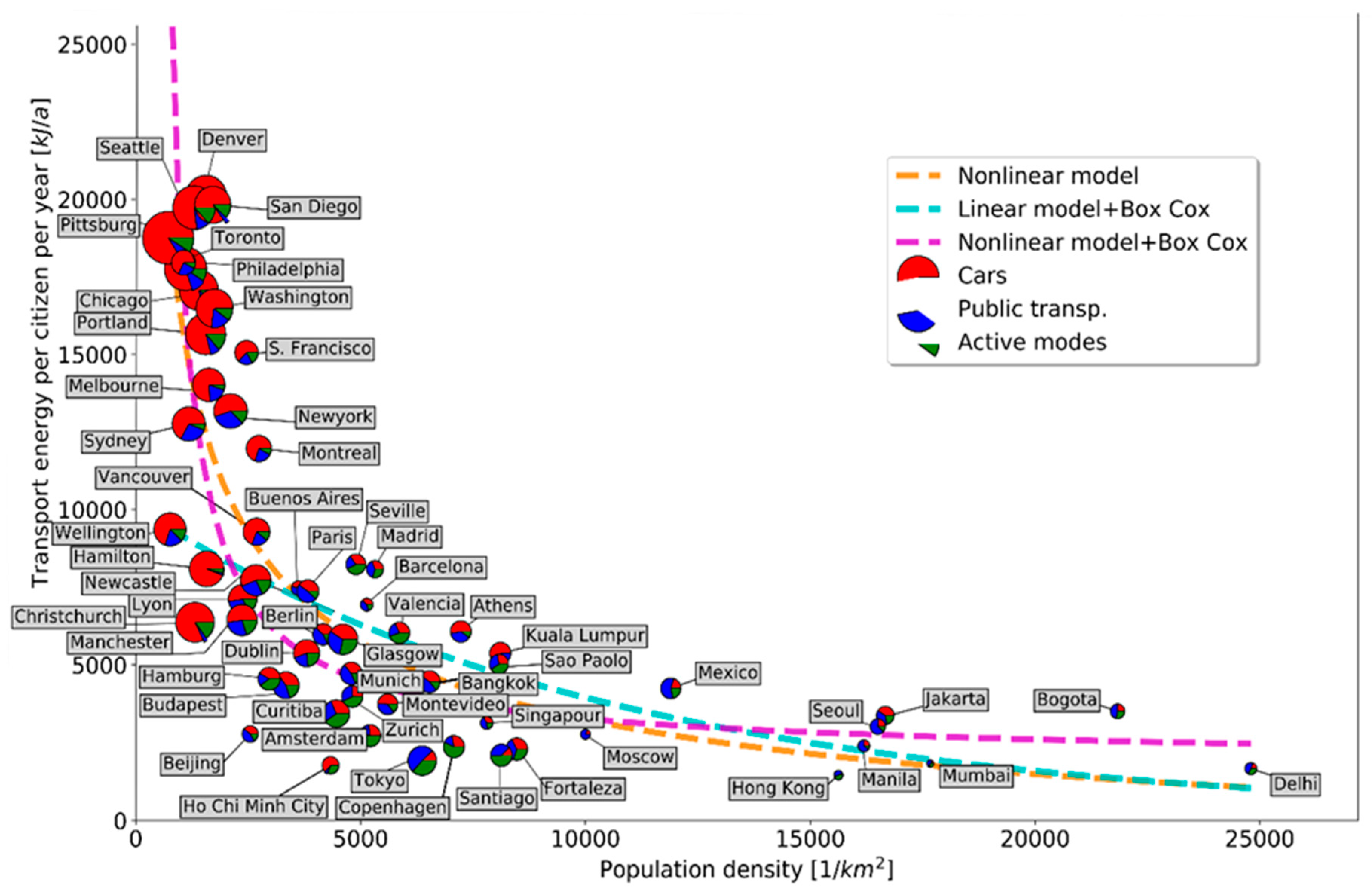
Figure 1 shows the transport energy WT and mode share versus the population density for each city. The same figure contains the hyperbolic shape of WT, which is similar to Newman and Kenworthy’s curve. A cluster of cities can be seen at low population densities between 1000–2500 persons/km2, where the majority are U.S. and Canadian cities. These low population density cities are showing a much higher transport related energy consumption compared with cities with higher population density. Low population density cities are also characterized by a high road infrastructure accessibility (see diameter of bubbles in Figure 1) and high car mode share (see pie chart of bubbles in Figure 1). Regarding mode shares of daily commuting in the U.S.: the private vehicle mode share is over 85% of all trips, which is followed by 5.2% share of public transportation trips [26]. Canadian, Australian and New Zealand cities, where car dependent mobility concepts are adopted, have, on average, slightly lower road infrastructure accessibility and slightly higher public transport usage compared with U.S. cities.
A cluster with mainly European, Latin American cities and some Asian cities such as Tokyo can be seen at population densities between 2500–8000 persons/km2 with medium level road infrastructure accessibility. Cities in this cluster consume noticeably less transport energy with respect to the first cluster. It is apparent that in this cluster, cities with the highest active mode share such as Tokyo, Amsterdam and Copenhagen consume the lowest transport energy. The cluster of cities with population densities above 8000 persons/Km2 are mainly Asian cities with low road infrastructure accessibility and a high public transport share.
The particularly sharp rise in energy consumption for decreasing population densities calls for some reasoning. The non-linear model shown in Figure 1 is developed in the following section.
3.2. Transport Infrastructure Population Density and Transport Energy Consumption
This section investigates how transport infrastructure and population density determine transport energy consumption, estimated in Equation (1). The road infrastructure accessibility (RIA) and other infrastructure accessibilities (rail-track infrastructure accessibility TIA and bike infrastructure accessibility BIA, which can be calculated with OSM data) are assumed to have an impact only on the respective mode shares MSC, MSPT and MSA, not on the other variables in Equation (1). The energy efficiency of private and public transport will not be part of the modeling.
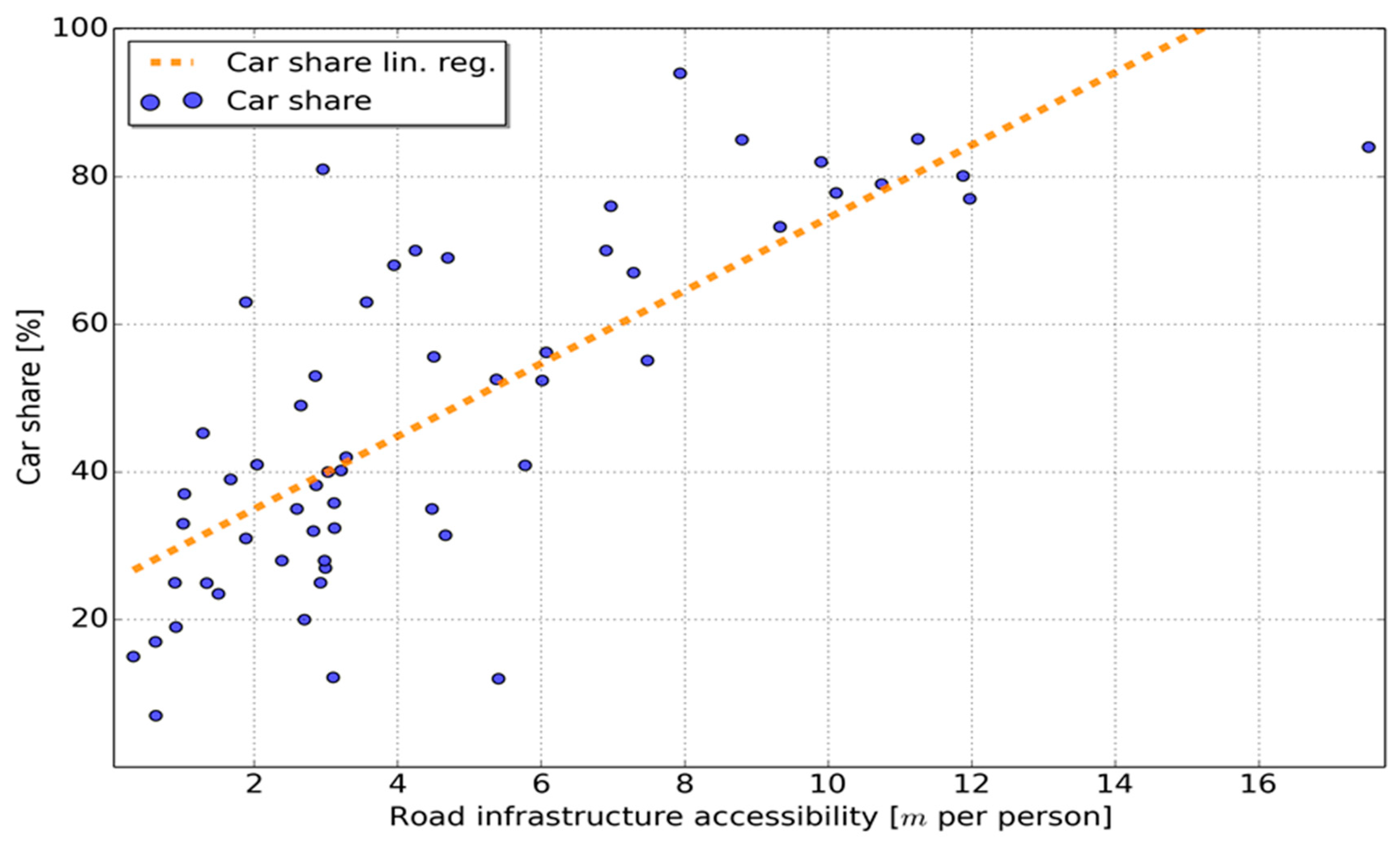
Concerning the MSC, the data shown in Figure 2 suggests a linear relation between road infrastructure accessibility RIA and car mode share MSC. The MSC has been estimated with the following equation:
where parameters have been estimated with a linear regression, see Table 1. The fit with is relatively good, considering the different error sources in the determination of RIA and MSC. The Harvey Collier test resulted in a p-value of 0.41, confirming that the null hypothesis that linear specification is correct should not be rejected. The skew is close to zero (0.198) and the p-value of the Jarque-Bera test is 0.62, indicating normally distributed residuals, even though there are uncertainties due to the small sample number. However, the reason why the road length per inhabitant increases car mode share in proportional way is not clear. In the literature, similar relations have been demonstrated empirically [6,7].
Regarding the public transport mode share MSPT, it is more difficult to establish a relation between the rail track length per inhabitant TIA and MSPT in the absents of more detailed information: the rail length represents only a part of all public transport infrastructures and in any case, the rail usage is only a share of all public transport trips. One interesting possibility is to test whether the MSPT depends also on the road infrastructure. Indeed, the linear approach has been tested:
with regression parameters and shown in Table 2. The results show that RIA is significant, and as is negative, an increasing RIA decreases public transport mode share, as expected. With the fitting is less pronounced with respect to Equation (2). The linear specification is correct as the p-vale of the Harvey Collier test equals 0.55 and it is likely that the residuals are normal distributed due to a skew close to zero and a Jarque-Bera p-value of 0.26.
Further modeling showed that also the bike mode share is negatively correlated with RIA.
The population density is assumed to influence the average daily commuting distances by car, DC, and the average daily commuting distances by public transport, DPT. The linear regression model:
shows that DC decreases with an increasing population density, parameters are statistically significant, but the fit is very weak as , see Table 3. The linear specification is correct as the p-vale of the Harvey Collier test equals 0.92. The residuals are likely to be normal distributed due to a skew close to zero (0.165) and a Jarque-Bera p-value of 0.77. The parameter has a relatively low absolute value, which means commute distances are slightly sensitive to the population density. The influence of the population density on the PT commute distance is not statistically significant for the present dataset.
Considering solely road infrastructure accessibility RIA and population density DPOP as independent variables, the transport energy estimate of a generic city shall be estimated by substituting the estimates of models from Equations (2)–(4) in the energy equation of Equation (1). The resulting energy estimate can be presented in the shape:
where the following parameters are assumed to be constant and independent from DPOP and RIA:
Note that the city index i of the various parameters in Equation (1) has been dropped and the respective quantities have been replaced by average values. The beta parameters in Equation (5) are determined by a linear regression instead of using the above equations, because doing so would lead to multiplicative errors. The regression results are presented in Table 4. This estimate is fitting well with the energy data as , and the signs of the parameters meet expectations. However, the parameter related to DPOP is not statistically significant and takes positive values within the 95% confidence interval. In addition, the independent variables are not homoscedastic as the p-value of the Breusch-Pagan Lagrange Multiplier test is a low A Box-Cox transformation of the model with the optimal lambda value of −0.036 is not able to improve this condition.
Dropping the explicit dependency on DPOP from Equation (5), one ends up with the simple transport energy estimate:
with the parameters and to be calibrated. However, as demonstrated below, RIA does depend on DPOP. The regression results in Table 5 demonstrate that both parameters are significant, with , which is only little worse than the model in Equation (5). The linear specification is correct as the p-vale of the Harvey Collier test equals 0.30. However, the residuals are unlikely to be normal distributed as the skew is different from zero (0.712) and the Jarque-Bera p-value is 0.012, which is below 0.05.
Any attempts to include rail-track infrastructure accessibility or bike infrastructure accessibility in the transport energy estimation resulted in a better fit of the energy data, but statistical significance is lacking.
3.3. The Relation between Population Density and Transport Energy Consumption
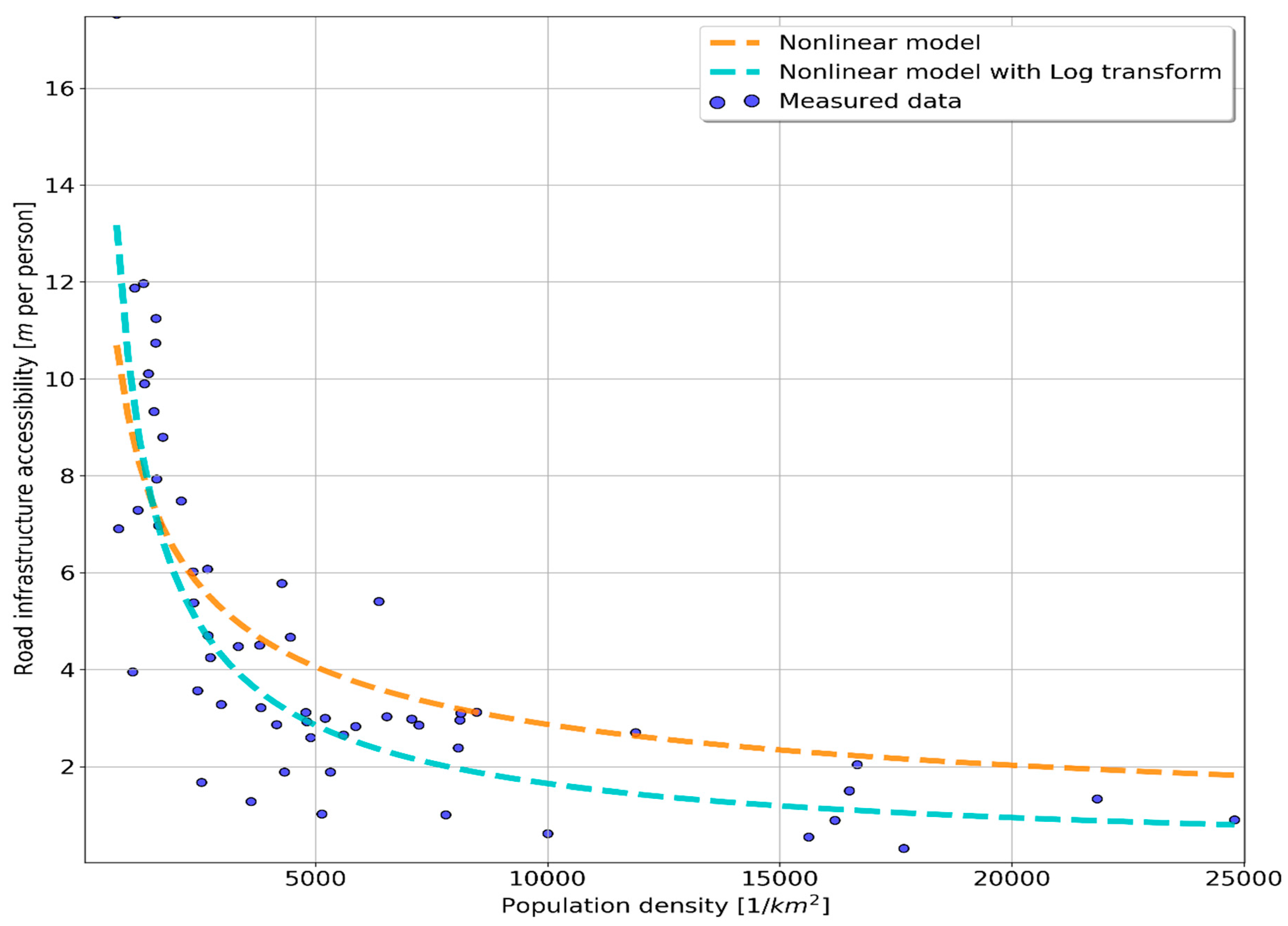
There still needs to be an explanation as to why the transport energy per person shown in Figure 1 is increasing so sharply for low population density. The previous section shows that the average travel distance DC is little sensitive to DPOP. Therefore, it must be the private car mode share MSC that increases in a non-linearly fashion as DPOP approaches zero. However, if the MSC increases linearly with RIA, as demonstrated in Section 3.1, then the relation between DPOP and RIA is necessarily of non-linear nature. In fact, Figure 3 shows that the RIA of the cities is rapidly decreasing as DPOP increases, similar to the transport energy curve in Figure 1.
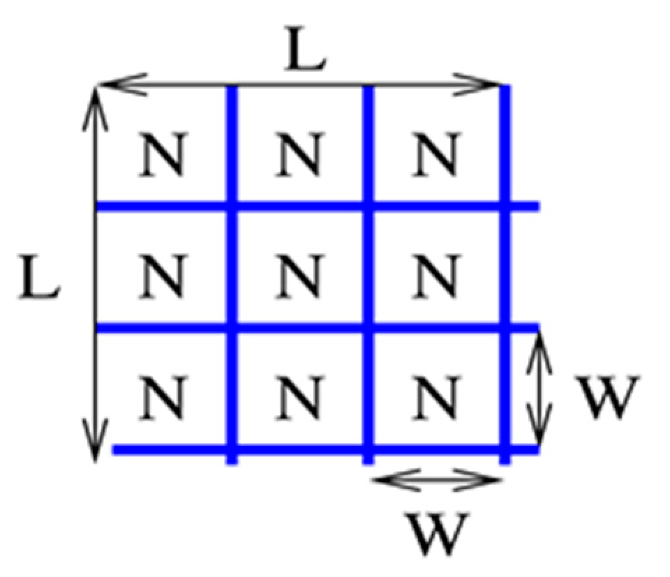
The following approximations are an attempt to explain why the road length per person tends to increase so dramatically for cities with low population density: assuming a city with a squared layout with side length L and a grid-like road network where all streets are W meters apart, as shown in Figure 4, of which the number of roads is in each coordinate and the total road length is .
Assuming further that the population is evenly spread over the city, then the population density is and the total population becomes As the road infrastructure accessibility is defined by , RIA is obtained by replacing W with :
where can be seen as a constant to be calibrated. Clearly, this equation determines the road length of a cities with varying population density, while limiting the road circuity constant to , which is a typical value for U.S. cities [39]. Note that RIA is dropping sharply for increasing DPOP, as expected from the city data. Applying an ordinary linear regression on the city data with DPOP in inhabitants per m2, the term is found to be statistically significant and within 0.256 and 0.316, using the 95% confidence interval. The average value of . Despite the simplicity of the grid-road model city, the estimate shows a goodness of fit with , even though the residuals are unlikely to be normal distributed as the skew is different from zero (0.856) and the Jarque-Bera p-value far below 0.05. The linear specification is correct as the p-vale of the Harvey Collier test equals 0.92.
It is worth mentioning that the estimate fits well because the calibration is determined by U.S. cities with a large RIA at low population densities and Asian cities with low RIA and high population densities, and just those dominant U.S. cities are the ones best represented by the regular road-grid that has been assumed in the above model.
The result of Equation (7) shall be verified by calibrating a non-linear model with a generic exponent of the shape:
and by comparing with the exponent 0.5 in Equation (7). With a log transformation, this problem can be transformed in a linear estimation problem of the form:
where and . The regression results of the log-model in Equation (9) are shown in Table 6. The linear specification is correct as the p-vale of the Harvey Collier test equals 0.24. However, the residuals are unlikely to be normal distributed as the skew is different from zero (−0.945) and the Jarque-Bera p-value well below 0.05.
Apparently, the exponent = 0.78 from Equation (8) is different from the exponent value of 0.5 in Equation (7), which represents the square root. Moreover, = 0.44 is different but in the same order of magnitude than from Equation (7). The goodness of fit of the model in Equation (8) with is marginally higher with respect to the model in Equation (7). These minor differences are not surprising, given the simplifying assumptions made during the derivation of Equation (7). The results of the two models are plotted in Figure 3.
As the derived model in Equation (7) reasonably explains the RIA of cities, Equation (7) is substituted into the energy estimate of Equation (6), which leads to a transport energy model as a nonlinear function of the population density. The shape of this transport energy estimate becomes:
with the parameters and to be calibrated with the transport energy data. The linear regression results in Table 7 indicate that both parameters are significant, the sign of is positive, as expected, and the fit is reasonable with . The linear specification is correct as the p-vale of the Harvey Collier test equals 0.24. The residuals are likely to be normal distributed due to a skew close to zero (−0.128) and a Jarque-Bera p-value of 0.41. This estimate explains the sharp rise of transport energies for low-density cities as previously shown in Figure 1.
In order to judge whether the particular non-liner shape of the model in Equation (10) is a reasonable fit, two other modeling attempts are investigated: first, a linear Box-Cox model of the form:
has been calibrated with an optimal . The parameters from Equation (11) are shown in Table 8. The outcome of the linearity test and the normal distribution test are equivalent to the results of the non-linear model from Equation (10). After a back-transformation of Equation (11), the obtained goodness of fit equals .
In a second attempt, a Box Cox transformed model with a non-linearity in has been calibrated, similar to the one in Equation (10):
With the previously optimized , the parameters from Equation (12) are shown in Table 9. The outcome of the linearity test and the normal distribution test are again identical to the non-linear model from Equation (10). After a back-transformation, the goodness of fit showed results in .
Apparently, the model in Equation (10) does best fit with the measured energy data. All three models of the transport energy estimation are shown in Figure 1.
3.4. Summarizing Discussion
Two quantities have been investigated, which can significantly influence the transport energy of cities, see Equation (1): the modal split and the average commute distance. From the present city dataset, there is statistical evidence that private commute travel distance is linearly decreasing with population density, see Equation (4). The model shows a ratio of approximately 50% between the commute distance of cities with highest and lowest population densities. However, the errors of this distance model are fairly large.
Regarding the mode shares, a significant, linear relation has been found between road infrastructure accessibility (RIA) and car mode share (MSC), see Equation (2). In this case, the ratio between MSCs of cities with the lowest and highest RIA is approximately 400%. This result means that RIA has a much stronger influence on the mode share than the population density has on the commute distance. The public transport infrastructure can only be represented by the rail length extracted from the OSM data of each city. This information proves insufficient to establish a relation between public transport infrastructure and public transport mode share MSPT, as rail constitutes only a part of all public transport trips. Instead, it has been possible to demonstrate that MSPT is decreasing linearly with RIA. The linear relations between RIA, MSC and MSPT have only been demonstrated empirically and a model to explain this relation quantitatively has not been found in literature. Nevertheless, as RIA does determine significantly both shares, MSC and MSPT, the transport energy has been estimated with a linear regression that depends only on RIA, see Equation (6). The failed attempts to include rail infrastructure accessibility (TIA) or bike infrastructure accessibility (BIA) in the transport energy estimation is probably due to the fact that both OSM data are insufficiently precise or incomplete to explain the public transport or active mode share, respectively. However, including rail and bike infrastructure accessibility reduces the errors in the model. Further tests have revealed that TIA actually increases proportionally with the rail mode share (for 17 cities, ) and BIA is proportional to bike mode share (for 32 cities, ). These findings support the relation between usage and alternative infrastructures expansion presumably by shifting car trips to alternative modes, as demonstrated in [43,44,45] for rail and in [46,47] for cycling. Better fits can be obtained when concentrating on a particular area: for example, the relation between BIA and the bike mode share has a better fit using only European cities with respect to cities from all countries available in the database. Still, the active-mode share includes walk-trips and walk infrastructure is difficult to assess with OSM data as footpath are generally insufficiently modelled in OSM.
In Section 3.2, a non-linear function between the population density and RIA has been derived from the data, based on a simplifying road-grid model, see Equation (7). This calibrated model fits well with empirical population density and RIA data and shows a marked rise of RIA as population density approaches zero. This model has been verified by calibrating a more generic model, whose parameters relaxed to values similar to the derived model of Equation (7). Combining the function in Equation (7) to compute RIA from the population density with the linear relation from Equation (6), which estimates the transport energy, it has been possible to calibrate a statistically significant model that estimates the transport energy as a function of the population density, see Equation (10). This model can explain the marked rise in transport energy for cities with low population density, as found already by Newman [5]. Nevertheless, there are some cities that do not fit well with the estimated energy curve: Hamilton, New Zealand, has a high car mode share (94%), but a relatively low energy use for its low population density. The reason is Hamilton’s relatively low average commute distance. Moreover, Ho Chi Minh City has short commute distances and, therefore, a relatively low transport energy consumption. Wellington has a low energy consumption for its population density, but as the metropolitan area has been used, the population density might be underestimated as most of the population lives in Wellington city. The Spanish cities Madrid, Seville and Barcelona have a relatively high transport energy consumption, despite a low car mode share, due to an exceptionally high commute distance.
Attempts to include the average commute distance as a linear function of the population density resulted in a slightly improved fit of the transport energy, but parameters became statistically insignificant and are not suited to explain the phenomenon.
4. Conclusions
Quality open source data from centralized databases allows for more consistent and complete analyses of transport networks from many cities around the world. Up to date information on urban area, population, average commute distances for private and public transport, specific energy consumption and modal splits have been obtained from different databases. Still, it has been challenging to obtain homogeneous data from a sufficient number of cities. City boundaries, sampling dates, and calculation methods of certain quantities were not homogeneous. Instead of eliminating a large quantity of cities due to insufficient data, it has been decided to estimate missing data from alternative sources, even though this may distort the results. It has been specified which data has been estimated with which method and for which city. The attribute rich information on transport infrastructure provided by Openstreetmap (OSM) has been used to extract the road length, rail length and bikeway length of the city’s transport networks by means of the open source software called OSMNx. From the collected city data, the transport related energy has been calculated, which is an important sustainability benchmark of the city’s transport system. The transport energy consumption essentially depends on two quantities: the modal split and the average commute distances.
The main focus of the analysis has been to establish a quantitative and statistically significant relation between population density, transport infrastructure and transport energy consumption. A particularity, already highlighted by Newman and Kenworthy [5], has been investigated: cities with low population density, from the U.S.A., Canada and Australia have an extraordinarily high transport energy consumption (2–4 time higher than medium density European or Asian cities). The result of present study has clearly identified the high private car mode share as main cause for the high transport energy usage of such cities, while the longer average commute distance in low-population density cities has a more modest influence on their transport energy consumption.
As a first step, a significant linear relation has been found between road length per inhabitant, the road infrastructure accessibility (RIA) and private car mode share: the car mode share increases with an increasing RIA, which is reasonable. There is also evidence for a linear relation between RIA and public transport mode share: in this case, the public transport mode share increases with a decreasing RIA, which suggests that people start using public transport if there are less road kilometers available per inhabitant. Furthermore, the results show that the average traveling distance by car is linearly decreasing with an increasing population density, a result that is significant, but shows large error bars. Based on these findings, a linear model for the transport energy consumption has been calibrated, where energy consumption increases with an increasing RIA. The inclusion of the population density as a linear term in the energy estimate did not show significant results. However, the city database shows that the population density has a strong, non-linear impact on RIA and therefore on the private car mode share and eventually also on the transport energy consumption.
As a second step, a simplified phenomenological model has been developed to explain the non-linear relation between the population density and RIA: RIA is dropping with one over the square root of the population density. Finally, based on this relation and the above findings, a function between the population density and the transport energy has been calibrated, which explains the rapid increase of transport energy consumption of cities with low population density.
One limitation of the presented models is surely the sole use of population density and road infrastructure length to explain transport energy consumption in cities. Such a simplification may hide the fact that transport energy consumption in cities with identical population density can vary considerably. Some examples were discussed where cities with low population density have a low energy density due to short commute distances. Another limitation is the use of inhomogeneous data; particularly the city boundaries are critical. The different criteria how city boundaries are drawn introduces large errors into the population density, thus impeding more refined analysis.
The overall conclusions of this work does confirm previous findings [5,6,8,9,10,11,12,13,14,15,16,17,18,19,20]. Cities with low population density must provide a disproportionately high road-length per inhabitant in order to cover the area and to limit longer de-tours with respect to the line of sight. This may suggest that line-oriented public transport cannot match the connectivity of the road network in low population density cities. In order to reduce the energy consumption in low density cities, either the energy efficiency of cars must increase, for example by battery electric vehicles. Otherwise, new forms of demand responsive public transport systems need to become competitive in low density settlement areas.
Cities with medium to high population densities do have either a substantial public transport mode share or a high active mode share or both. This fact leads, on average, to a lower energy consumption with respect to cities with low population density. The study has not covered quantitatively the role of cycling and bicycle infrastructure such as bike share has not been available for most cities. However, cities with the lowest transport energy consumption do almost all have a high share of active modes, including cycling.
Author Contributions
Conceptualization, A.E.D. and J.S.; Methodology, A.E.D. and J.S.; Software, A.E.D.; Validation, J.S.; Analysis, A.E.D. and J.S.; Investigation, A.E.D.; Data Curation, A.E.D.; Writing-Original Draft Preparation, A.E.D.; Writing-Review & Editing, F.R., J.S. and Z.S., Visualization, A.E.D. and J.S.; Supervision, F.R. and Z.S.
Funding
This research received no external funding.
Conflicts of Interest
The authors declare no conflict of interest.
References
- Haustein, K.; Allen, M.R.; Forster, P.M.; Otto, F.E.L.; Mitchell, D.M.; Matthews, H.D.; Frame, D.J. A real-time global warming index. Sci. Rep. 2017, 7, 15417. [Google Scholar] [CrossRef] [PubMed]
- International Energy Agency (IEA). World Energy Outlook 2012; International Energy Agency, OECD/IEA: Paris, France, 2012; p. 690. ISBN 978-92-64-18084-0. [Google Scholar]
- International Energy Agency (IEA). Policy Pathways: A Tale of Renewed Cities; International Energy Agency: Paris, France, 2013; p. 98. [Google Scholar]
- International Energy Agency (IEA). CO2 Emissions from Fuel Combustion, Highlights; International Energy Agency: Paris, France, 2011; p. 66. [Google Scholar]
- Newman, P.W.G.; Kenworthy, J.R. The transport energy trade-off: Fuel-efficient traffic versus fuel-efficient cities. Transp. Res. 1988, 22, 163–174. [Google Scholar] [CrossRef]
- Brownstone, D.; Golob, T.F. The impact of residential density on vehicle usage and energy consumption. J. Urban Econ. 2009, 65, 91–98. [Google Scholar] [CrossRef] [Green Version]
- Os’orio, B.; McCullen, N.; Walker, I.; Coley, D. Understanding the relationship between energy consumption and urban form. Athens J. Sci. 2017, 4, 115–142. [Google Scholar] [CrossRef]
- Crane, R. The influence of urban form on travel: An interpretive review. J. Plan. Lit. 2000, 15, 3–23. [Google Scholar] [CrossRef]
- Limtanakool, N.; Dijst, M.; Schwanen, T. The influence of socioeconomic characteristics, land use and travel time considerations on mode choice for medium- and longer-distance trips. J. Transp. Geogr. 2006, 14, 327–341. [Google Scholar] [CrossRef]
- Dingil, A.E.; Schweizer, J.; Rupi, F.; Stasiskiene, Z. Transport indicator analysis and comparison of 151 urban areas, based on open source data. Eur. Transp. Res. Rev. (ETRR) 2018, 10, 58. [Google Scholar] [CrossRef]
- Ingram, G.; Liu, Z. Determinants of motorization and road provision. In Essays in Transportation Economics and Policy; Ibanez, G., Tye, B.W., Winston, C., Eds.; Brookings Institution Press: Washington, DC, USA, 1999; pp. 325–356. [Google Scholar]
- Melo, P.S.; Graham, D.J.; Canavan, S. Effects of road investments on economic output and induced travel demand evidence for urbanized areas in the United States. Transp. Res. Rec. 2012, 2297, 163–171. [Google Scholar] [CrossRef]
- Chakour, V.; Eluru, N. Examining the influence of urban form and land use on bus ridership in Montreal. Procedia-Soc. Behav. Sci. 2013, 104, 875–884. [Google Scholar] [CrossRef]
- Kenworthy, J.; Laube, F. Automobile dependence in cities: An international comparison of urban transport and land use patterns with implications for sustainability. Environ. Impact Assess. Rev. 1996, 16, 279–308. [Google Scholar] [CrossRef]
- Chen, C.; Gong, H.; Paaswell, R. Role of the built environment on mode choice decisions: Additional evidence on the impact of density. Transportation 2008, 35, 285–299. [Google Scholar] [CrossRef]
- Kitamura, R. A dynamic model system of household car ownership, trip generation, and modal split: Model development and simulation experiment. Transportation 2009, 36, 711–732. [Google Scholar] [CrossRef]
- Baum-Snow, N.; Brandt, L.; Henderson, J.V.; Turner, M.A.; Zhang, Q. Roads, Railroads and Decentralization of Chinese Cities. Rev. Econ. Stat. 2012, 99, 435–448. [Google Scholar]
- Baum-Snow, N. Did highways cause suburbanization? Q. J. Econ. 2007, 122, 775–805. [Google Scholar] [CrossRef]
- Chi, G.Q. The impacts of highway expansion on population change: An integrated spatial approach. Rural Sociol. 2010, 75, 58–89. [Google Scholar] [CrossRef]
- Cervero, R. Road Expansion, Urban Growth, and Induced Travel: A Path Analysis. J. Am. Plan. Assoc. 2003, 69, 145–163. [Google Scholar] [CrossRef]
- Citypopulation. Database. 2019. Available online: http://www.citypopulation.de (accessed on 1 October 2018).
- Organisation for Economic Co-operation and Development (OECD). Working Age Population. 2019. Available online: https://data.oecd.org/pop/working-age-population.htm (accessed on 15 October 2019).
- Statista. Database. 2019. Available online: https://0-www-statista-com.brum.beds.ac.uk/ (accessed on 15 October 2019).
- European Environment Agency. Infrastructure Density and Accessibility by Country. 2018. Available online: https://www.eea.europa.eu/data-and-maps/daviz/infrastructure-density-and-accessibility-per-country-1 (accessed on 16 October 2019).
- Boeing, G. OSMnx: New Methods for Acquiring, Constructing, Analyzing, and Visualizing Complex Street Networks. Comput. Environ. Urban Syst. 2017, 65, 126–139. [Google Scholar] [CrossRef]
- American Fact Finder. Database. 2019. Available online: https://factfinder.census.gov/faces/nav/jsf/pages/searchresults.xhtml?refresh=t (accessed on 20 February 2019).
- Eurostat. Database. 2018. Available online: http://ec.europa.eu/eurostat/web/cities/data/database?p_p_id=NavTreeportletprod_WAR_NavTreeportletprod_INSTANCE_KhPDfq283AOB&p_p_lifecycle=0&p_p_state=normal&p_p_mode=view&p_p_col_id=column-2&p_p_col_count=1 (accessed on 20 February 2019).
- Development Bank of Latin America (CAF). Database. 2019. Available online: https://www.caf.com/es/conocimiento/datos (accessed on 22 February 2019).
- New Zealand Stats. Transport Database. 2019. Available online: http://nzdotstat.stats.govt.nz/wbos/Index.aspx (accessed on 23 February 2019).
- Urban Land Institute. A ULI Advisory Services Panel Report. 4–9; Urban Land Institute: Moscow, Russia, 2011. [Google Scholar]
- Urbanage. LSE Cities Database. 2018. Available online: https://urbanage.lsecities.net/data (accessed on 10 December 2018).
- EPOMM. Database. 2019. Available online: http://www.epomm.eu/tems/ (accessed on 15 January 2019).
- Statistics Canada. Database. 2019. Available online: http://www12.statcan.gc.ca/census-recensement/2016/dp-pd/prof/index.cfm?Lang=E&TABID=1 (accessed on 22 February 2019).
- Australian Bureau of Statistics, Australian Government. 2016. Available online: http://stat.data.abs.gov.au/ (accessed on 15 December 2018).
- LTA Academy. “Passenger Transport Mode Shares in World Cities” JOURNEYS. 2014. Available online: http://www.lta.gov.sg/ltaacademy/doc/J14Nov_p54ReferenceModeShares.pdf (accessed on 15 October 2018).
- Worldbank. Urban Transport Data Analysis Tool (UT-DAT). 2019. Available online: http://www.worldbank.org/en/topic/transport/publication/urban-transport-data-analysis-tool-ut-dat1 (accessed on 15 March 2019).
- Moovit. Commute Distance Traveled by Public Transit Database. 2019. Available online: https://moovitapp.com/insights/en/Moovit_Insights_Public_Transit_Index-commute-distance (accessed on 15 March 2019).
- Statistics Netherlands. Report: Travel and Mobility 2016. 2016. Available online: https://www.cbs.nl/-/media (accessed on 20 March 2019).
- Cycling-Embassy of Denmark Report: Copenhagen City of Cyclists. 2011. Available online: http://www.cycling-embassy.dk/wp-content/uploads/2011/05/Bicycle-account-2010-Copenhagen.pdf (accessed on 15 March 2019).
- Elizabeth Kneebone and Natalie Holmes. The Growing Distance between People and Jobs in Metropolitan America. Brookings Metropolitan Policy Program. 2015. Available online: https://www.brookings.edu/wp-content/uploads/2016/07/Srvy_JobsProximity.pdf (accessed on 20 March 2019).
- Boscoe, F.P.; Henry, K.A.; Zdeb, M.S. A nationwide comparison of driving distance versus straight-line distance to hospitals. Prof. Geogr. 2012, 64, 188–196. [Google Scholar] [CrossRef] [PubMed]
- Kenworthy, J.R. Energy Use and CO2 Production in the Urban Passenger Transport Systems of 84 International Cities: Findings and Policy Implications. In Urban Energy Transition: From Fossil Fuels to Renewable Power—Chapter 9; Elsevier: Amsterdam, The Netherlands, 2011. [Google Scholar]
- Urban Transportation Group. Rail Cities UK: Our Vision for Their Future. Report. 2018. Available online: http://www.urbantransportgroup.org/resources/types/reports/rail-cities-uk-our-vision-their-future (accessed on 20 February 2019).
- Lee, S.S.; Senior, M.L. Do light rail services discourage car ownership and use? Evidence from Census data for four English cities. J. Transp. Geogr. 2013, 29, 11–23. [Google Scholar] [CrossRef]
- Hass-Klau, C.; Crampton, G.; Biereth, C.; Deutsch, V. Bus or Light Rail: Making the Right Choice: A Financial, Operational, and Demand Comparison of Light Rail, Guided Busways and Bus Lanes; Environmental & Transport Planning: Brighton, UK, 2004. [Google Scholar]
- Dill, J.; Carr, T. Bicycle commuting and facilities in major U.S. cities: If you build them, commuters will use them. Transp. Res. Rec. 2003, 1828, 116–123. [Google Scholar] [CrossRef]
- Schweizer, J.; Rupi, F. Performance Evaluation of Extreme Bicycle Scenarios. Procedia-Soc. Behav. Sci. 2013, 111, 508–517. [Google Scholar] [CrossRef]
Figure 1.
Transport related energy consumption per person in one year for commuting purposes in city i (, over population density (DPOP). For each city, also the modal split is shown: the share of private car transport (MSC) in red, the public transport share (MSPT) in blue and the active mode share (MSA) in green. The bubble size is proportional to the road infrastructure accessibility (RIA) of the respective city. The dashed lines represent different models which are derived in Section 3.2: The nonlinear model from Equation (10) (dashed orange), the linear model with Box Cox back-transform from Equation (11) (dashed light blue) and the nonlinear model with Box-Cox back-transformation from Equation (12) (dashed magenta).

Figure 2.
Car mode share (MSC) over road infrastructure accessibility (RIA). The blue bubbles represent the car shares from the city database, while the dashed orange line represents a linear regression model from Equation (2) ().
Figure 2.
Car mode share (MSC) over road infrastructure accessibility (RIA). The blue bubbles represent the car shares from the city database, while the dashed orange line represents a linear regression model from Equation (2) ().

Figure 3.
Road infrastructure accessibility RIA over population density DPOP. The orange dashed line represents the non-linear function of Equation (7) with a goodness of fit of . The light blue dashed line represents the back transformed Log model from Equations (8) and (9) with a goodness of fit of .

Figure 4.
Simplified squared city with a street grid of roads in x-direction and the same number of roads in y-direction. In each sub-square of size live N citizens.
Figure 4.
Simplified squared city with a street grid of roads in x-direction and the same number of roads in y-direction. In each sub-square of size live N citizens.


Table 1.
Linear regression results for private car mode share in Equation (2). The table shows the parameter values (coef), the standard error (Std. err.), the t-value (t), the probability to exceed the absolute of the t-value and the 95% confidence interval of the parameter values (95.0% Conf. Int.).
| Coef | Std. err. | t | P > |t| | 95.0% Conf. Int. | ||
|---|---|---|---|---|---|---|
| 25.12 | 3.320 | 7.567 | 0.000 | 18.470 | 31.778 | |
| 4.93 | 0.570 | 8.642 | 0.000 | 3.787 | 6.073 | |
Table 2.
Linear regression results for public transport mode share (MSPT) in Equation (3).
| Coef | Std err | t | P > |t| | 95.0% Conf. Int. | ||
|---|---|---|---|---|---|---|
| 46.177 | 2.816 | 16.396 | 0.000 | 40.533 | 51.821 | |
| −3.372 | −6.971 | 0.484 | 0.000 | −4.342 | −2.403 | |
Table 3.
Linear regression results for average commute travel distance in Equation (4).
| Coef | Std err | t | P > |t| | [95.0% Conf. Int.] | ||
|---|---|---|---|---|---|---|
| 31.0955 | 1.697 | 18.326 | 0.000 | 27.695 | 34.496 | |
| −0.0006 | 0.000 | −2.917 | 0.005 | −0.001 | 0.000 | |
Table 4.
Linear regression results for transport energy consumption per person per year of Equation (5).
Table 4.
Linear regression results for transport energy consumption per person per year of Equation (5).
| Coef | Std err | T | P > |t| | 95.0% Conf. Int. | ||
|---|---|---|---|---|---|---|
| 5.077 × 10⁶ | 1.32 × 10⁶ | 3.854 | 0.000 | 2.43 × 10⁶ | 7.72 × 10⁶ | |
| −3.628 × 10⁵ | 1.16 × 10⁶ | −0.312 | 0.757 | −2.7 × 10⁶ | 1.97 × 10⁶ | |
| 1.196 × 10⁵ | 1.62 × 10⁴ | 7.402 | 0.000 | 8.72 × 10⁴ | 1.52 × 10⁵ | |
| −1.788 × 10⁵ | 6.98 × 10⁴ | −2.562 | 0.013 | −3.19 × 10⁵ | −3.88 × 10⁴ | |
Table 5.
Linear regression results for average commute travel distance in Equation (6).
| Coef | Std err | t | P > |t| | 95.0% Conf. Int. | ||
|---|---|---|---|---|---|---|
| 1.91 × 10⁶ | 7.58 × 10⁵ | 2.519 | 0.015 | 3.9 × 10⁵ | 3.43 × 10⁶ | |
| 1.24 × 10⁵ | 1.3 × 10⁴ | 9.520 | 0.000 | 9.79 × 10⁴ | 1.5 × 10⁵ | |
Table 6.
Linear regression results for road infrastructure accessibility in Equation (9).
| Coef | Std err | t | P > |t| | [95.0% Conf. Int.] | ||
|---|---|---|---|---|---|---|
| −3.1318 | 0.408 | −7.668 | 0.000 | −3.950 | −2.313 | |
| −0.7890 | 0.073 | −10.797 | 0.000 | −0.935 | −0.643 | |
Table 7.
Linear regression results for the transport energy in Equation (10).
| Coef | Std err | T | P > |t| | 95.0% Conf. Int. | ||
|---|---|---|---|---|---|---|
| −2.735 × 10⁶ | 1.12 × 10⁶ | −2.439 | 0.018 | −4.98 × 10⁶ | −4.88 × 10⁵ | |
| 5.983 × 10⁸ | 5.93 × 10⁷ | 10.082 | 0.000 | 4.79 × 10⁸ | 7.17 × 10⁸ | |
Table 8.
Box-Cox linear regression results for transport energy in Equation (11).
| Coef | Std err | t | P > |t| | [95.0% Conf. Int.] | ||
|---|---|---|---|---|---|---|
| −2.735 × 10⁶ | 1.12 × 10⁶ | −2.439 | 0.018 | −4.98 × 10⁶ | −4.88 × 10⁵ | |
| 5.983 × 10⁸ | 5.93 × 10⁷ | 10.082 | 0.000 | 4.79 × 10⁸ | 7.17 × 10⁸ | |
Table 9.
Linear regression results for transport energy in Equation (12).
| Coef | Std err | t | P > |t| | [95.0% Conf. Int.] | ||
|---|---|---|---|---|---|---|
| −2.735 × 10⁶ | 1.12 × 10⁶ | −2.439 | 0.018 | −4.98 × 10⁶ | −4.88 × 10⁵ | |
| 5.983 × 10⁸ | 5.93 × 10⁷ | 10.082 | 0.000 | 4.79 × 10⁸ | 7.17 × 10⁸ | |
© 2019 by the authors. Licensee MDPI, Basel, Switzerland. This article is an open access article distributed under the terms and conditions of the Creative Commons Attribution (CC BY) license (http://creativecommons.org/licenses/by/4.0/).
Share and Cite
MDPI and ACS Style
Dingil, A.E.; Schweizer, J.; Rupi, F.; Stasiskiene, Z. Updated Models of Passenger Transport Related Energy Consumption of Urban Areas. Sustainability 2019, 11, 4060. https://0-doi-org.brum.beds.ac.uk/10.3390/su11154060
AMA Style
Dingil AE, Schweizer J, Rupi F, Stasiskiene Z. Updated Models of Passenger Transport Related Energy Consumption of Urban Areas. Sustainability. 2019; 11(15):4060. https://0-doi-org.brum.beds.ac.uk/10.3390/su11154060
Chicago/Turabian StyleDingil, Ali Enes, Joerg Schweizer, Federico Rupi, and Zaneta Stasiskiene. 2019. "Updated Models of Passenger Transport Related Energy Consumption of Urban Areas" Sustainability 11, no. 15: 4060. https://0-doi-org.brum.beds.ac.uk/10.3390/su11154060
Note that from the first issue of 2016, this journal uses article numbers instead of page numbers. See further details here.