CFD Simulation of Convective Heat Transfer on Vernacular Sustainable Architecture: Validation and Application of Methodology

Abstract

The global background of energy shortages and climate deterioration demands bioclimatic sustainable buildings. Vernacular architecture can provide a useful resource of passive strategies and techniques for creating inner comfort conditions with minimum heating, ventilation, and air conditioning (HVAC) assistance. The identification and verification of such knowledge are essential for climate responsive or energy passive building design. Among the methods, computational fluid dynamics (CFD) is a useful tool for simulating convective heat transfer of vernacular architecture and predicting the convective heat transfer coefficient (CHTC) and flow field. Geometric complexity and diversity of building samples are crucial in the development of an effective simulation methodology in terms of computational cost and accuracy. Therefore, this paper presents high-resolution 3D steady Reynolds-averaged Navier–Stokes (RANS) CFD simulations of convective heat transfer on Japanese vernacular architecture, namely, “machiya.” A CFD validation study on the CHTC is performed based on wind-tunnel experiments on a cube heated by constant heat flux and placed in a turbulent channel flow with a Reynolds number of 3.3 × 10⁴. Three steady RANS models and two boundary layer modeling approaches are compared and discussed. Results show that the SST k-ω model applied with low Reynolds number modeling approach is suitable for CHTC simulations on a simplified building model. The RNG k-ε model applied with wall functions is an appropriate choice for simulating flow field of a complicated building model. Overall, this study develops a methodology involving RANS model selection, boundary layer modeling, and target model fitting to predict the convective heat transfer on vernacular architecture.

1. Introduction

Approximately 40% of global energy is consumed in buildings [1], and 50% of building energy is used to maintain indoor comfort by utilizing heating, ventilation, and air conditioning (HVAC) auxiliary systems [2]. The depletion of energy resources and the risk of climate changes (i.e., global warming, melting glaciers, heavier rainstorms, more frequent drought. etc.) demand a sustainable development path based on renewable energies and energy efficiency. One of the most substantial issues is designing and constructing buildings that can provide inner comfort conditions by optimizing the use of natural resources. Consequently, the pollution usage of HVAC auxiliary systems can be reduced to a minimum.

Climate responsive or energy passive building designs can play a significant role in reducing the energy demand of buildings without compromising modern living standards. The so-called “bioclimatic approach to architecture” started with the research of Victor Olgyay (1963) [3], which aims to achieve optimal comfort preferably using architectural elements and avoid complete dependence on mechanical systems. Although the term “bioclimatism” appeared as late as the mid-20th century, the bioclimatic approach in architecture can be traced back to the passive design principles applied in worldwide vernacular architecture. The lack of artificial means, such as HVAC, required past designers to build houses by completely utilizing the opportunities offered by the climates [4]. These design principles or strategies were developed by “trial and error” and passed down for hundreds of years, leading to the diversity of architectural forms in response to the worldwide climates. In summary, the analysis of vernacular architecture, the knowledge of which has been accumulated for centuries, is fundamental to understanding the climatic behavior of a building in its environment and adapting this knowledge to current societal customs.

Before application to modern architecture, the effects and mechanisms of these strategies and techniques should be scientifically studied. The key steps of the research on vernacular architecture have gone through stages from empirical methods to analytical and computational modeling methods. Until the 1960s, these methods were summarized into scientific publications [3,5]. Scientific studies of the adaption of these methods to modern architecture started in 1977 [6]. After the 1990s, numerical simulation was applied to validate and verify building performance with the support of advanced computer technology [7].

The convective heat transfer on the building surface is of scientific and practical interest in the analysis of vernacular architecture. Especially in the field of architectural environmentalism, airflow has a considerable influence on heat loss and surface temperature at the external and internal building surfaces [8]. Convective heat transfer of the external building surface transmits heat to the atmosphere, which is one of the main reasons for formation of urban heat island effect and energy losses in buildings [9,10]. The internal convection of buildings affects temperature distribution of indoor air, buoyancy-driven flow motion, and mean radiant temperature, affecting human comfort [11,12]. Normally, convective heat transfer at a building surface is modeled by the convective heat transfer coefficient (CHTC, $h_c$) [8,12,13,14,15,16,17,18]. The CHTC ($h_c$) relates the convective heat flux (q) to the difference between surface temperature $T_s$ and environmental air temperature $T_a$.

$$h_c=\frac{q}{\left(T_s-T_a\right)},$$

(1)

The CHTC is important in assessing the energy performance of vernacular architecture and is used to calculate the convective heat losses. Substantial research has focused on the formulation of models to estimate the CHTC. Based on wind tunnel experiments on convective heat transfer on flat plates [19,20,21] and bluff bodies [22,23,24,25], as well as field measurements for building facades [13,26,27,28,29,30], several correlations have been developed and widely applied in modeling, simulations, and calculations for building energy consumption. However, the CHTC at the facade of a building is complex and influenced by a wide range of parameters, including building geometry [31], building surroundings [32], discrete measurement position on the building façades [17,18], facade roughness [33], wind speed, and wind direction [34,35]. All these experiments and field measurements somehow have their shortcomings in terms of limited physical similarity regarding the flow pattern, architectural shapes and boundary conditions. Therefore, these case-specific correlations have the limitation of applicability in the energy analysis of vernacular architecture.

Computational fluid dynamics (CFD) has recently become another option for predicting CHTC on building surfaces [15,16,17,18,32,35]. One of the main advantages of CFD lies in its ability to obtain high spatial resolution for a specific and complicated architectural shape. That is, CFD simulations can easily provide a sufficient amount of local CHTC distributions of each building surface prior to using empirical equations or field measurements. In addition, the flow and temperature fields are available. Previous studies mostly used steady Reynolds-averaged Navier–Stokes (RANS) to model the flow and temperature fields compared with unsteady RANS (URANS) or large-eddy simulations (LES). The RANS equations govern the transport of the averaged flow quantities, with the whole range of the scales of turbulence being modeled. The RANS model, therefore, greatly reduces the required computational effort and resources, and is widely adopted for practical engineering applications. In terms of CHTC prediction, previous studies normally focused on simple shapes (i.e., cubes) [31]. However, in the simulation of vernacular architecture, the building geometry can be relatively complex, and the number of cases can be quite large. Therefore, an effective and relatively accurate methodology is required. That is, turning the problem into a balance between computational cost and accuracy is a concern of architects and engineers. Another factor that affects simulation effectiveness is the modeling of the near-wall region, which includes low-Reynolds number modeling (LRNM) and wall function approaches. For LRNM, a very high grid resolution with high computational cost is required near the wall. Wall functions are commonly used instead because of their low grid requirement. However, the accuracy of wall functions must be validated in terms of the convective heat transfer issue.

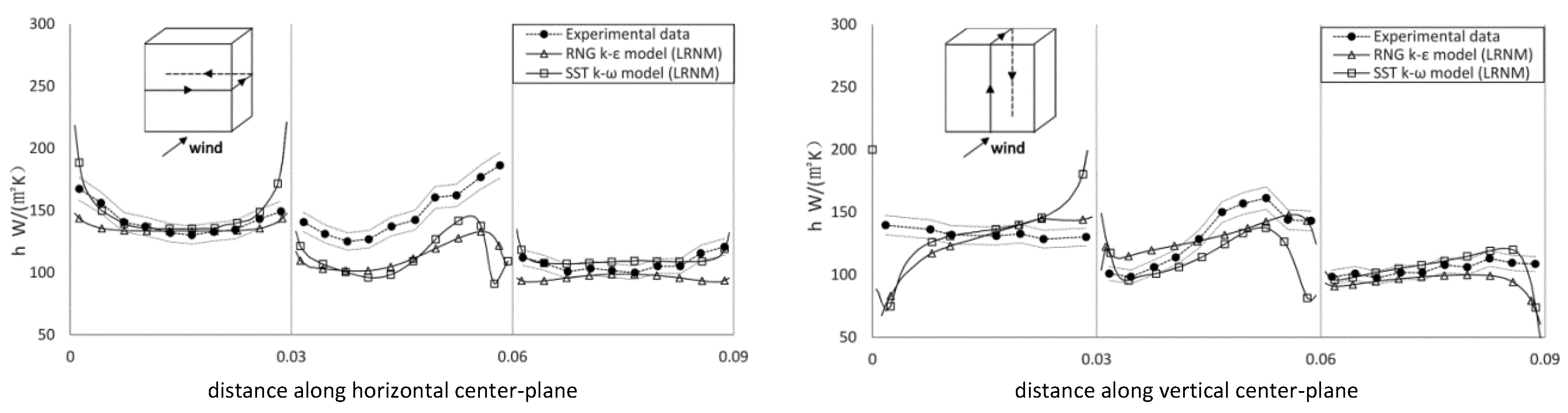
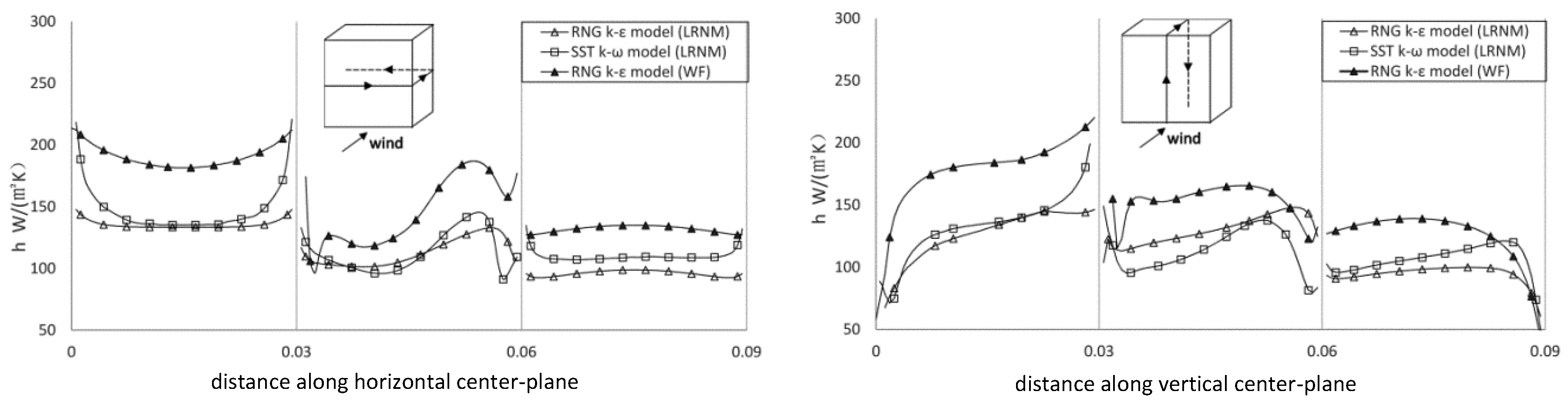
The main aim of the study presented in this paper is to seek an appropriate methodology for simulating the convective heat transfer in vernacular architecture considering computational cost and accuracy. First, a CFD validation study on the CHTC is performed based on wind-tunnel measurement of a wall-mounted cube immersed in a turbulent boundary layer. Three steady RANS models (namely, the standard k-ε (sk-ε), re-normalization group k-ε (RNG k-ε), and shear-stress transport k-ω (SST k-ω) models) and two boundary layer modeling approaches (wall functions and low-Reynolds number modeling) are compared and discussed. The details of the numerical simulation are described in Section 2, and the simulation results are discussed in Section 3. Next, a typical architecture form of vernacular architecture in Nala, Japan, namely, “machiya,” is simulated as an application example. The “machiya” is a typical case of Japanese vernacular architecture, which organizes effective cross ventilation to reduce indoor humidity and hotness. The convective heat transfer accounts for a large part of the heat losses in “machiya”, which is the main reason it is selected and simulated. The simulation results of the CHTC are compared with different empirical correlations, and the flow field verifies the ventilation technique, indicating that “machiya” is equipped to adapt to the climates. The conclusions are provided in Section 5.

2. Numerical Simulation

2.1. Turbulence Modeling

OpenFOAM, which is applied to the control volume method, is used in the simulations. Three different two-equation turbulence models of steady RANS, namely, the sk-ε, RNG k-ε, and SST k-ω models, are accessed with the LRNM approach. The RNG k-ε model is also evaluated with the wall functions approach.

2.2. Boundary-Layer Modeling

According to previous studies, the sk-ε model is valid in areas where turbulence is fully developed but performs poorly in near-wall regions [36]. As presented in the last section, such problems can be dealt with in two ways: LRNM and wall functions approach.

Wall functions are normally empirical equations used to satisfy the physics of the flow in the near-wall region. The theory of wall functions applied in OpenFOAM is based on the research of Georgi Kalitzin [37]. The inner region between the wall and the flow, namely, the viscous layer, the buffer layer, and a part of the log-low layer, is not resolved using wall functions [38]. The advantages include a considerable reduction in mesh amount and the turbulence domain. Instead, the first cell center must be placed in the log-law region, with a normal $y^{+}$ value ranging from 30 to 500 to ensure the accuracy of simulations. Dimensionless parameters $y^{+}$ and $u^{+}$ are usually used to express wall functions:

$$y^{+}=\frac{y\times u_{\tau }}{\nu },$$

(2)

$$u_{\tau }=\sqrt{\frac{{\tau }_{\omega }}{\rho }},$$

(3)

$$u^{+}=\frac{u}{u_{\tau }},$$

(4)

where $y^{+}$ is the non-dimensional distance to the wall; $u_{\tau }$ is the friction velocity, which is used to define dimensionless velocity $u^{+}$; and ${\tau }_{\omega }$ is the wall shear stress. The viscosity and density of fluid used in Equations (3) and (4) are represented by $\nu$ and $\rho$, respectively. The wall functions applied in OpenFOAM and used in this work are nutKwallfuction and alphatJayatillekeWallFunction, which respectively denote velocity and temperature resolution.

In contrast to wall functions, the LRNM approach integrates the turbulence to the wall. The turbulence models are modified to resolve the viscosity-affected region with all the mesh down to the wall, including the viscous sublayer. The SST k-ω model is developed to compensate for the shortcomings of the k-ε model in near-wall resolution, which uses a k-ω formulation in the near-wall region and switches to the k-ε formulation in the free-stream. Therefore, the turbulent core region of the flow is resolved with the k-ε model, and a low-Reynolds number model is used to resolve the viscosity-affected region. LRNM grids typically require the placement of the first cell center in the viscous sublayer (normally $y^{+}<5$ and preferably $y^{+}=1$). This approach requires a considerable mesh amount, especially in the case of high Reynolds numbers or complicated geometries, indicating the need for a substantial computational resource.

2.3. Heat Transfer Modeling

The steady-state solver, buoyantBousinessqSimpleFoam, which is provided by OpenFOAM and developed for buoyant, turbulent flow of incompressible fluids, is applied in this work. In flows accompanied by heat transfer, the fluid properties are normally functions of temperature. The variation may be small but can cause fluid motion. The Boussinesq approximation treats the density as a constant in unsteady and convection terms and only as a variable in the gravitational term in case of small density variation. Thus, the governing equations can be expressed as follows:

$$\mathrm{Continuity}\mathrm{equation}:\nabla ·\left(u\right)=0,$$

(5)

$$\mathrm{Momentum}\mathrm{equation}:\frac{\partial \left(u\right)}{\partial t}+\nabla ·\left(uu\right)=-\nabla p_{rgh}-\left(g·r\right)\nabla \left(\frac{\rho }{{\rho }_0}\right)+\nabla ·\left(2v_{eff}D\left(u\right)\right),$$

(6)

$$\mathrm{Temperature}\mathrm{equation}:\nabla ·\left(Tu\right)=k_{eff}{\nabla }^{2}T,$$

(7)

where u is the velocity field, p is the pressure field, ρ is the density field, and g is the gravitational acceleration. The effective kinematic viscosity ($v_{eff}$) is the sum of the molecular and turbulent kinematic viscosities. The effective thermal conductivity of air ($k_{eff}$) is the sum of thermal and turbulent thermal conductivity:

$$v_{eff}=v+v_t,$$

(8)

$$k_{eff}=k+k_t=\frac{v}{pr}+\frac{v_t}{P{r}_t}.$$

(9)

The turbulent thermal conductivity is proportional to the turbulent kinematic viscosity ($v_t$). All parameters and air properties reported in this paper are defined in

Table 1. Air properties and parameters used in the simulations.

Dynamic Viscosity (kg·m−1·s−1)	1.831 × 10−5
Specific heat capacity (J·kg−1·K−1)	1004.4
Thermal expansion coefficient (K−1)	0.00341
Prandtl number	0.72
Turbulent Prandtl number	0.85
Temperature (K)	293.15

.

3. Numerical Simulation

3.1. Experimental Details

The experiment on convective heat transfer at the surfaces of a cube placed in a turbulent layer, which was studied by Nakamura et al. [23], is used for validation purposes. A cube with a height (d) of 30 mm was set in a low-speed wind channel with a working section, which was 400 mm high, 300 mm wide, and 800 mm long (Figure 1). Experiments were performed at several free-stream velocities ($u_0$) ranging from 2.2 m/s to 17.3 m/s. For the validation study, a free-stream velocity of 16.6 m/s with Reynolds number of 3.3 × ${10}^4$ based on the cube height was considered. The turbulent boundary layer with a turbulent intensity of 0.5% was achieved by attaching a circular cylinder of 10 mm in diameter on the floor at 500 mm upstream from the cube. The boundary layer thickness (δ) was 45 mm when the Reynolds number was 3.3 × ${10}^4$.

In terms of local heat transfer measurement, the cube and the floor were fabricated with acrylic resin plates and covered with stainless steel sheets, which were electrically connected in series and heated by constant heat flux. The thermocouples were attached on the exterior and interior surfaces of the cube to measure the temperature gradient of the exterior surfaces and estimate the heat loss by conduction from the heater to the acrylic resin. Overall uncertainty for the heat transfer coefficient was reported to be within 5.5%.

3.2. Numerical Model

The streamwise, normal, and spanwise lengths of the three-dimensional computational domain are 17d, 9d, and 26d, respectively (Figure 2). The blockage ratio is 0.65%. Experimental data of the inlet flow can be used to provide realistic inlet conditions for the numerical simulations [23]. The free-stream turbulence intensity is 0.5%. The temperature of the inlet flow is 20 °C, which is taken as the reference temperature. A zero static pressure is imposed as the outlet boundary condition. The plate and the exterior surfaces of the cube are modeled as no-slip boundaries and taken as fixed heat flux for the temperature boundary conditions, which are consistent with the experimental settings. The top, left and right surfaces of the domain are taken as slip and modeled as zero gradient for the temperature boundary conditions.

Two mesh systems are generated using the structured grid in Pointwise according to general RANS practice. The cell density in the near-wall region is dependent on the boundary layer modeling. For Cases 1, 2, and 3 using the LRNM, a high cell density in the wall-normal direction and a small $y^{+}$ value for the first cell ($y^{+}=1$) are required. Therefore, the grids, which comprise 3.83 × 10⁶ cells, are fine in the near-wall region. The highest $y^{+}$ values smaller than 2 appear at the edges of the cube. For Case 4, wall functions are applied and fewer cells are generated (1.98 × 10⁶ cells), satisfying the $y^{+}$ value as required ($30<y^{+}<500$). The calculation conditions are summarized in

Table 2. Calculation condition.

	RANS Model	Boundary-Layer Modeling	Mesh System
Case. 1	sk-ε	LRNM	LRNM
Case. 2	RNG k-ε	LRNM	LRNM
Case. 3	SST k-ω	LRNM	LRNM
Case. 4	RNG k-ε	WF	WF

.

3.3. Results and Discussion

3.3.1. Flow Field

The flow field structure around the cube in the turbulent flow exhibits complex phenomena, such as separation, recirculation, and reattachment, which were presented by Meinders et al. and shown in Figure 3 [39]. Sketch of flow along center line (z = 0) of the experiment is shown in Figure 4. Figure 5 shows the time-averaged streamlines on the symmetry plane (z = 0) and floor plane (y = 0) for numerical methods. Although some differences are visible, the general flow features and the overall prediction of the front, top, and rear vortex modes are evidently similar. The fluid flow separates in the near windward edge of the top and lateral faces owing to the increase in fluid pressure and decrease in fluid velocity. The main vortex forms a horseshoe-type vortex around the cube and interacts with the main separation region behind the cube. Nakamura et al. and Meinders et al. observed flow reattachment on the top face, which is not exhibited by most of the simulations. The windward separation point of the horseshoe-type vortex is initiated in front of the cube (marked S) with distance $X_1$. In the rear of the cube, the shear layer separated at the top leading edge reattaches at point R with a separation length ($X_2$). According to the experiment data, the windward separation point (S) is located at $X_1=1.04d$, and the flow reattaches in the rear region where separation length $X_2=1.5d$. The front stagnation point is z = 0, and $L_1$ = 0.6d on the front face of the cube. The reverse flow separates at the upstream region of $L_2$ = d/6, and an upward flow is formed at $L_3$ = 0.15d on the rear face.

The details of the flow field characteristics are summarized in

Table 3. Values of characteristic length of flow vertex.

	${\mathit{X}}_1$	${\mathit{X}}_2$	${\mathit{L}}_1$	${\mathit{L}}_2$	${\mathit{L}}_3$
Case. 1	0.583d	2.313d	0.684d	0.021d	0.147d
Case. 2	0.75d	2.75d	0.696d	0.208d	0.174d
Case. 3	0.771d	2.814d	0.638d	0.181d	0.204d
Case. 4	0.75d	3.17d	0.66d	0.148d	/
Exp.	1.04d	1.5d	0.6d	0.167d	0.15d

. The results show that the RANS model could not generally reproduce the details of the separation of the boundary layer in front of the cube nor the reattachment behind the cube, resulting in a short $X_1$ and a long $X_2$. This inability is commonly believed to be due to the disregard of unsteady effects, such as vortex shedding. In terms of the second vortex, the application of the RNG k-ε and the SST k-ω models with the LRNM approach simulates the flow structure better than that of the sk-ε model. Therefore, the RNG k-ε (Case 2) and SST k-ω (Case 3) models are selected and compared in the prediction of the CHTC in the next section.

3.3.2. Heat Transfer by Low-Reynolds Number Modeling (LRNM)

In Figure 6, the local CHTC distribution of Case 2 and Case 3 in the vertical and horizontal center-plane of the cube surfaces is plotted for numerical simulations and experiments. The results show the quantitative agreement of the CHTC at the windward and leeward surfaces between numerical and experimental data, except for some discrepancies at the downward region. However, some considerable discrepancies occur at the top and lateral surfaces of the cube. The differences with experimental data can be partially attributed to the effect of the heat transfer at the ground whose boundary conditions are simplified in the numerical simulations. In addition, the limitation of the number of thermocouples in terms of cube size can result in low resolution of the experimental data of surface temperatures, especially in the edge regions.

The RNG k-ε and SST k-ω models perform well in the windward and leeward regions. A good agreement is obtained in the mid of vertical and horizontal center-planes of the windward surfaces. However, different degrees of discrepancies appear at the edge zones. The heat transfer obtained by Meinders et al. showed extreme values of CHTC near edges of the cube, which were not found in the profile of Nakamura et al. possibly due to the low resolution of the experiments in the edge zones. At the windward surface, the SST k-ω model shows better results than those of the RNG k-ε model. At the leeward surface, the SST k-ω model presents a similar tendency to the experimental data, with the CHTC slightly increasing from mid to side. However, the RNG k-ε model exhibits an opposite tendency. In terms of the value of CHTC, the SST k-ω model matches better in the edge region than the RNG k-ε model, which shows better results in the mid region.

For the top and lateral surfaces, although considerable discrepancies are found in the value of CHTC, the SST k-ω and RNG k-ε models present a similar tendency to the experimental data. At the top surface, according to the experiment of Nakamura, the CHTC is the maximum in the reattachment region of the shear layer and the minimum in the separation vortex region. Meinders attributed this phenomenon to the relatively high air temperature in the core of the separation vortex, which decreases the heat transfer. The low-enthalpy air impinges on to the surface, which results in a relatively high heat transfer rate [39]. On the top surface, the SST k-ω model shows better results in the location of separation and reattachment and the value of CHTC. At the lateral surfaces, a minimum CHTC is obtained at the separation region. To some extent, the RNG k-ε model shows better results in the location of separation and tendency than those in the SST k-ω model. The discrepancies at the top and lateral surfaces, which predict the low value of CHTC, are most likely related to the characteristics of the RANS models, of ignoring flow unsteadiness in turbulence resolution. The simulations conducted by Defraeye et al. (2010) showed similar results. Notably, the accuracy of CHTC can be increased by using other modeling techniques, such as URANS or LES [40]; however, these techniques are not the interest of this study.

3.3.3. LRNM versus Wall Functions

Figure 7 shows a comparison of the CHTC values over the vertical and horizontal center planes between Cases 2 and 3 using the LRNM and Case 4, which is applied with wall functions. At almost every surface of the cube, Cases 4 and 2 show a similar tendency, but using wall functions yields a discrepancy of up to 50%. Wall functions, which allow avoidance of high-resolution computational grids and thus have less computational cost and time, are relatively weak at CHTC estimation on the building surface. One of the most important reasons for compensating for these discrepancies relies on the wall functions, which are based on certain assumptions when dealing with near-wall resolution. That is, wall functions do not resolve the viscous sublayer and the buffer layer, wherein the largest resistance to surface heat transfer is embedded. Launder claims that the abandonment of the wall function approach resulted in marked improvement in the prediction of convective heat transfer rates [36]. Wall functions should generally not be applied in simulations focused on near-wall region resolution, which is the exact case for convective heat transfer at building surfaces. However, wall functions still have some advantages, such as resolution of the velocity and temperature fields inside the domain. Figure 8 shows the normalized time-averaged stream-wise velocity (a) and temperature (b) profile at different positions on the y = 0 plane. The comparisons show that although wall functions exhibit some considerable deviations on CHTC prediction, they still obtain similar fluid flow, velocity, and temperature fields to those in the LRNM, especially in regions far from the wall.

4. Application: Simulations of Vernacular Architecture

Considering the use of empirical equations or CFD simulations to predict the CHTC, previous studies normally focused on simple architectural shapes (such as cubes). However, in the case of specific buildings, the complexity of building geometries has a crucial impact on the flow field and convective heat transfer at surfaces [31]. Especially in the simulation of vernacular architecture, building geometries can be complicated, and the number of building samples can be large. On the one hand, the CHTC of each surface of the building, which is crucial for computing building energy consumption, should be accurately calculated. On the other hand, architects must perceive the flow field inside and outside the building to validate the passive methods and strategies applied in vernacular architecture, which do not require precise simulations. Therefore, the estimation of the CHTC of buildings and the wind fields outside and inside buildings is actually a trade-off between accuracy and efficiency. According to the results of the above validation, a specific case, that is, the Japanese vernacular architecture “machiya,” is introduced as an application.

4.1. Introduction of “Machiya”

Japan climate has a wide spectrum from summer to winter; however, its vernacular architecture is developed for summer. The doors and partitions between wooden columns are flimsy and lead to poor insulation. Consequently, some portable, local heating devices (such as stoves) are applied to compensate for the heat loss in winter, thus providing an acceptably comfortable indoor environment. By contrast, surviving in summer without active artificial devices is crucial. The city of Nara is crowded and surrounded by mountains, which although protects it from typhoons, gives little ventilation, turning its summers into a torrid, humid and suffocating experience. The “machiya” includes a series of elements and spaces that allow the cross-ventilation of rooms to deal effectively with the high humidity and hotness. A unique space, “doma,” with an earthen floor all through the length of “machiya,” is made in each house to enable good ventilation (Figure 9a). With no fixed separation between rooms, wind entering from the outside street can freely travel through different rooms. The window at the upper side wall of the house induces air current based on the air buoyancy effect due to the temperature difference, removing indoor hotness and humidity. By the time the wind reaches a small central courtyard, its temperature has risen and is lifted naturally through the courtyard into the atmosphere (Figure 9b). “Machiya” uses reasonable building shape and space organization and a series of passive strategies to form passive systems. On this basis, the cross-ventilation is strengthened, thereby improving human comfort. Such effects and mechanism can be validated by CFD simulation.

4.2. Simulation for CHTC

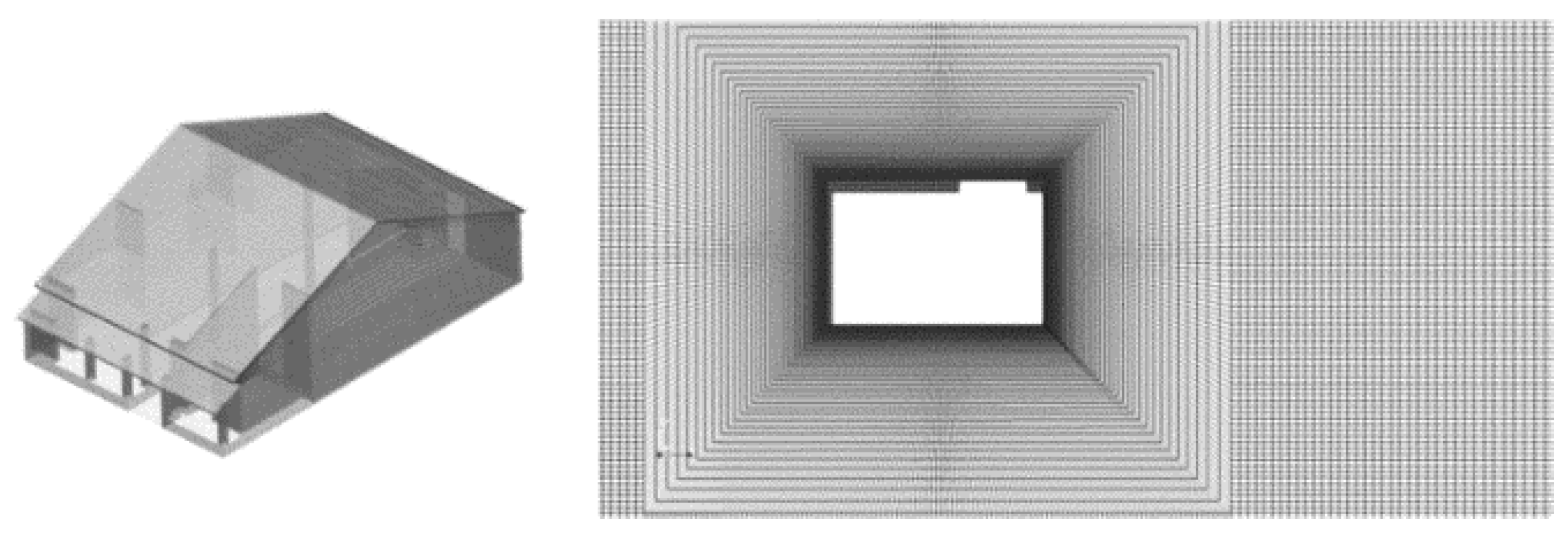
As stated in the previous section, the calculation of the CHTC demands the LRNM approach to resolve the viscous layer heat transfer. That is, a fine mesh generation satisfying the $y^{+}$ requirement to be approximately 1 is necessary. Consequently, a simplified modeling strategy is adopted to avoid high computational cost and time. In addition, the SST k-ω model is preferred according to the validation results.

Figure 10 shows the computational domain and mesh system of the simplified model. Only the external surfaces are modeled, and $y^{+}$ at the surfaces is limited to be less than 3. The streamwise, normal, and spanwise lengths of the three-dimensional computational domain are 9, 6, and 15 D, respectively (D = 8 m). The total cell number is approximately 7 million. As reported, the average CHTC value of buildings strongly depends on the ambient wind velocity magnitude [14]. In this work, the inflow conditions are based on the dominant wind direction and average wind velocity of the local location (Nara, lat: 34.69, lon: 135.80). A turbulent flow ($u_0=3.6\mathrm{m}/\mathrm{s}$, $R_e=1.95\times {10}^6$) is imposed at the inlet of the computational domain with a 0° angle. The temperature of the inlet wind flow is 20 °C, with a temperature difference of approximately 10 °C between the wall and the wind flow.

Figure 11 shows the velocity and temperature fields of the “machiya” house at the vertical center plane (y = 0) and the horizontal plane (z = 1/4D). The average CHTCs of each surface are summarized in

Table 4. Calculation condition.

	Face. 1	Face. 2	Face. 3	Face. 4	Face. 5	Face. 6	Face. 7	Average
	15.65 w/(m2K)	12.62 w/(m2K)	18.09 w/(m2K)	13.98 w/(m2K)	9.68 w/(m2K)	12.50 w/(m2K)	12.14 w/(m2K)	12.38 w/(m2K)

. A comparison with four correlations developed from field measurements (

Table 5. Expressions of different correlations and the calculation results of “machiya”.

Models	Correlations	$\mathbf{Results}({\mathit{u}}_{10}=3.6 \mathbf{m}/\mathbf{s})$
Loveday and Taki	$h_c=16.15\times {\left(0.68u_{10}-0.5\right)}^{0.397}$	21.04 w/(m2K)
ASHRAE task group	$h_c=18.6\times u_{10c}{}^{0.605}$ $u_{10c}=0.5, u_{10}<2 \mathrm{m}/\mathrm{s}$ $u_{10c}=0.25u_{10}, u_{10}>2 \mathrm{m}/\mathrm{s}$	17.45 w/(m2K)
MoWITT	$h_c=\sqrt{{[C_t{\left(T_s-T_a\right)}^{1/3}]}^2+{(a{u}_{10}^b)}^2}$	7.66 w/(m2K)
Liu and Harris	$h_c=1.53u_{10}+1.43$	6.94 w/(m2K)
Defraeye Blocken	$h_c=5.14u_{10}^{0.82}$	14.69 w/(m2K)
McAdams	$h_c=5.7+3.8u_{10}U<5 \mathrm{m}/\mathrm{s}$	19.38 w/(m2K)

) is performed to validate the CFD numerical model. The correlation was developed from flat-plate experiments by McAdams and numerical simulations by Defraeye et al. In the CFD simulations, $u_{10}$ corresponds to the wind velocity magnitude assigned at the inlet boundary condition ($u_0$).

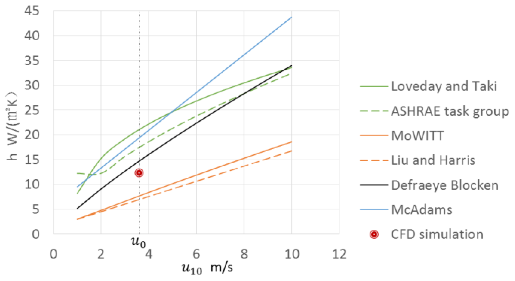
The CFD simulation obtains a big separation at the roof ridge, developing a large separation region behind the house. The high turbulence intensity and the low wind velocity lead to a weak heat transfer rate [40], which can be validated by the simulation results. The windward half part of the sloping roof generally has a larger CHTC than that of the leeward half part. In addition, the windward vertical walls have a larger CHTC than that of the leeward vertical walls. The four models developed from field measurements can be separated into two groups: Loveday and Taki [27] and the ASHRAE (American Society of Heating, Refrigerating and Air-Conditioning Engineers) task group [41] is representative of high buildings with six to eight floors, while the MoWITT [42] and Liu and Harris [29] group is representative of low-rise buildings. Figure 12 shows the CHTC profiles with the wind velocity measured at 10 m above the ground level in the upstream undisturbed wind flow (${\mathrm{u}}_{10}$). The CFD simulation achieves an intermediate value between the two groups of models. The discrepancies in these empirical correlations indicate that although the wind tunnel experiments and field measurements can provide realistic CHTC profiles, they usually lead to case-specific correlations. In terms of large varieties of building geometries and boundary conditions, such correlations cannot simply be applied to each case, which can be confirmed again by the deviation between the CFD simulation and the widely used correlation by McAdams. The numerical correlation of Blocken shows a similar but slightly larger CHTC value than that in the simulation results, which can be partly attributed to the difference between building geometries.

4.3. Simulation for Flow Field

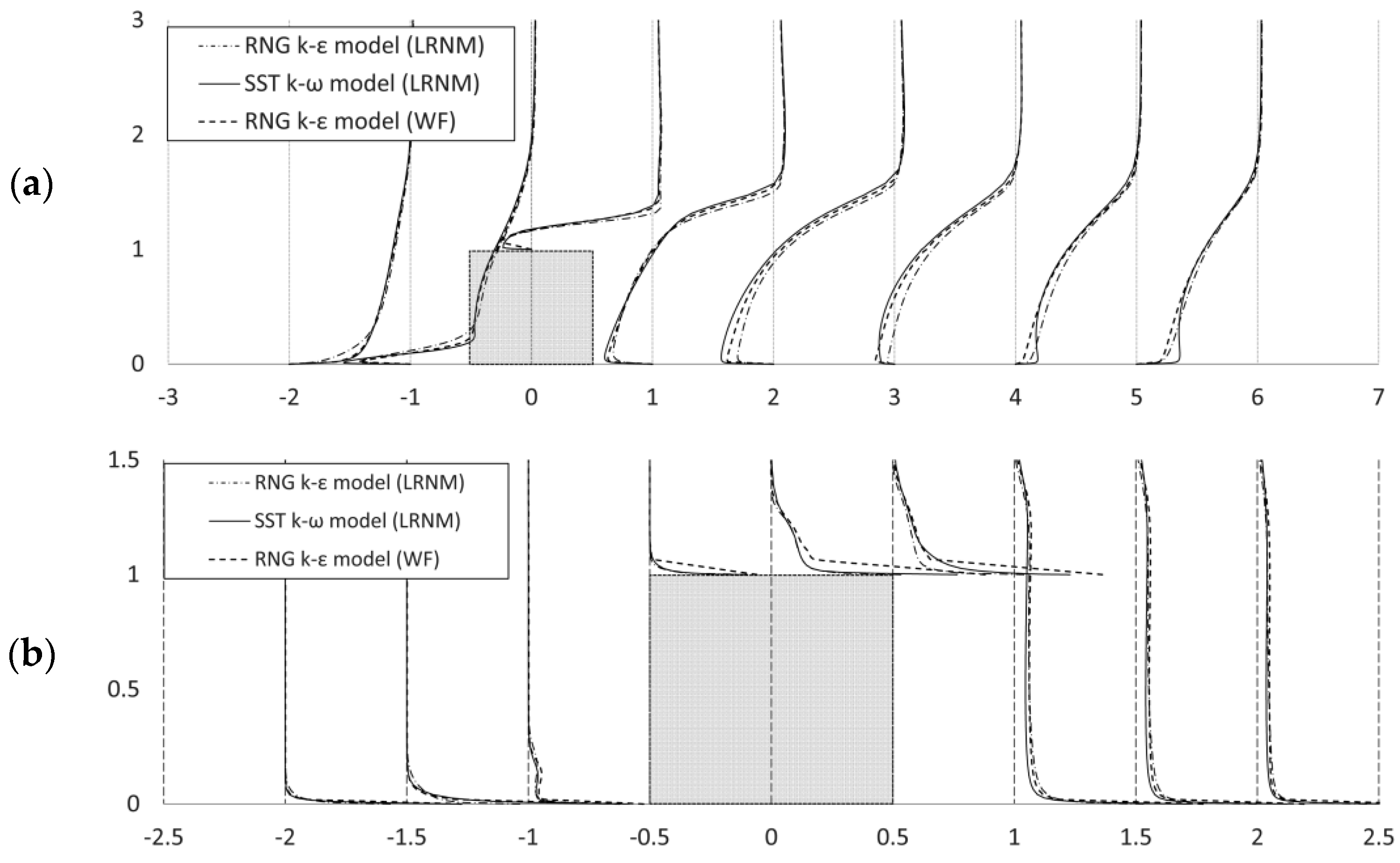
As confirmed in the validation, although simulations using wall functions cannot precisely calculate the CHTC, the solution of velocity and temperature field is highly consistent with the simulations applied with the LRNM approach. Therefore, resolving the fluid flow and temperature distribution of complicated models with low computational cost using wall functions is possible. The RANS model, the RNG k-ε model, is thus selected.

In the simulation of the flow field of “machiya” house, a rough grid system is generated with $y^{+}$ > 30. The complicated model and computational domain are shown in Figure 13. External and internal surfaces are modeled. The size of the computational domain is the same as that of the simplified case but with a total cell number of 5.5 million. The inflow condition is also the same as that in the simplified case, with a uniform flow ($u_0=3.6\mathrm{m}/\mathrm{s}$, $R_e=1.95\times {10}^6$) imposed vertically facing the building.

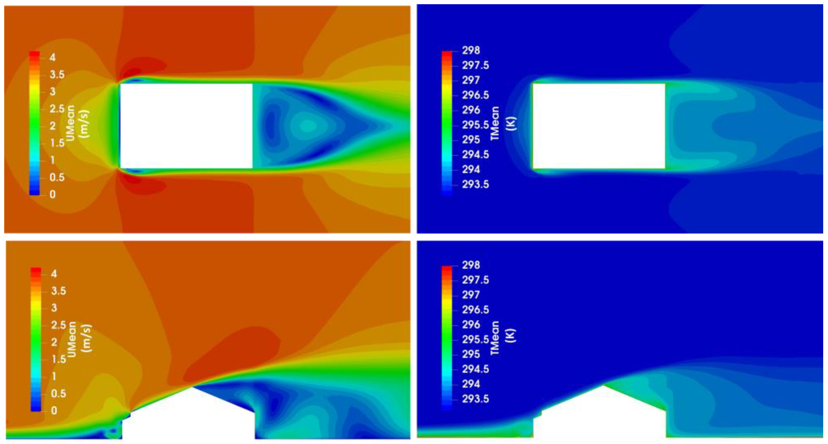
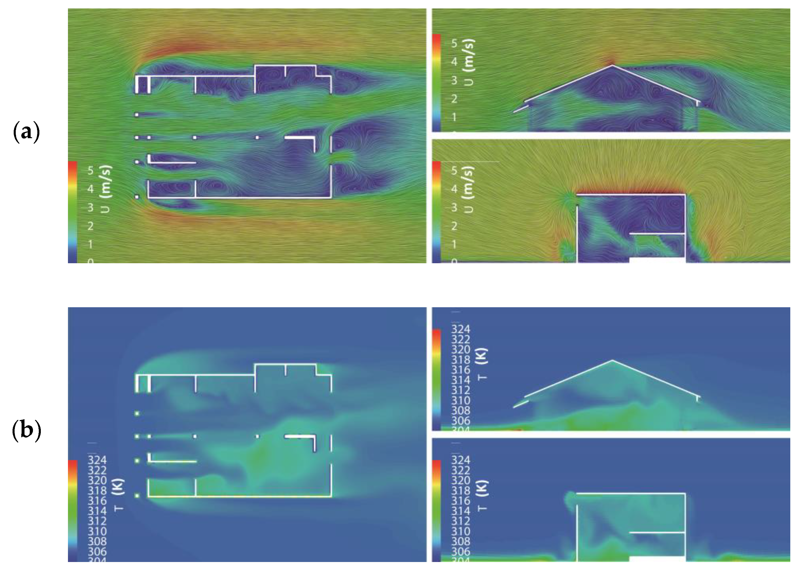
The temperature and velocity fields are shown in Figure 14. The difference in wind pressure between the windward and leeward regions allows the airflow to pass through the building and remove the hot air from indoors to outdoors. In general, the corner space, which is highly enclosed, easily forms eddy currents, leading to the low efficiency of convective heat transfer and ventilation. The ventilation and heat exchange at a relatively open space is better, especially when the front and rear openings are opposite. In addition, a highly enclosed room with small openings has an even slower wind velocity, lower temperature, and heat transfer rate than that of open space. Even when some doors are closed for privacy reasons, the “doma” space still acts like a wind tunnel that activates cross-ventilation (Figure 15a). The air is gradually heated when passing through the room. In this process, the air density decreases and the buoyancy effect lifts the hot air, which finally passes through the window on the sidewall (Figure 15b).

Notably, a deviation exists between the outdoor flow fields of the complicated and simplified models, which is determined by the model fineness and the influence of the indoor flow. Furthermore, the influence of local interferences and microclimatic conditions can be major to simulation results, however it is intentionally ignored in the application study. Although these simplifications will inevitably affect the prediction of the actual CHTC, the accuracy of the simplified model is within an acceptable tolerance according to the validation results.

5. Conclusions

Assessing the thermal and airflow environments in vernacular architecture is of considerable importance in validating and generating climate responsive or energy passive strategies. Specifically, the CHTC at the external surfaces of a building is an important parameter for the accurate numerical simulations of the thermal and airflow environments.

In the validation study, three RANS models and two boundary layer modeling are compared and analyzed in detail. For the CHTC prediction, RANS models applied with the LRNM approach are more accurate than those applied with wall functions. Using wall functions yields a discrepancy of up to 50% compared with the experimental data. The SST k-ω model with the LRNM approach shows better performance in predicting the CHTC than the RNG k-ε and sk-ε models, especially on the windward and leeward surfaces. Given that steady RANS modeling cannot fully consider the flow unsteadiness because of its time-averaged nature, the flow separation and recirculation region cannot be resolved precisely. Consequently, the CHTCs on the lateral and rear surfaces are relatively smaller than those of experimental data, with a discrepancy of approximately 14.3%. Nevertheless, the SST k-ω model applied with the LRNM approach can predict the distribution of the CHTC value over each surface of the building, which is a remarkable improvement to precisely calculating the building energy consumption. Although wall functions exhibit a considerable deviation in CHTC prediction, they still obtain consistent fluid flow, velocity, and temperature fields compared with those of the LRNM, especially in regions far from the wall.

This study developed a methodology involving RANS model selection, boundary layer modeling, and fitness of a target model to predict the convective heat transfer in terms of accuracy and computational cost to demonstrate the application of CFD simulations for CHTC and flow fields. In the simulation of the CHTC, the SST k-ω model applied with the LRNM approach requires a large amount of mesh cells and a short time-step, incurring high computational cost and time. In this case, the building model must be simplified to improve the efficiency of the operation. Furthermore, the fineness of the building model has more influence on the flow field than the CHTC. In the flow field simulation, the RNG k-ε model applied with wall functions is an appropriate choice in terms of its advantage of considerably reducing the computational cost and time. The validation and application indicate that CFD simulation can provide relatively accurate CHTC and flow field for specific and complicated vernacular architecture, laying the foundation for future studies to identify and verify the performance of bioclimatic strategies in vernacular sustainable architecture. These strategies would be committed to optimize the geometries and forms of sustainable architecture, in response to the global background of energy shortage and climate deterioration.

References

1. Sun, B.; Luh, P.B.; Jia, Q.S.; Jiang, Z.; Wang, F.; Chen, S. Building Energy Management: Integrated Control of Active and Passive Heating, Cooling, Lighting, Shading, and Ventilation Systems. IEEE Trans. Autom. Sci. Eng. 2013, 10, 588–602. [Google Scholar]
2. Pérez-Lombard, L.; Ortiz, J.; Pout, C. A review on buildings energy consumption information. Energy Build. 2008, 40, 394–398. [Google Scholar] [CrossRef]
3. Olgyay, V.; Olgyay, A. Design with Climate: Bioclimatic Approach to Architectural Regionalism. Some Chapters Based on Cooperative Research with Aladar Olgyay; Princeton University Press: Princeton, NJ, USA, 1963. [Google Scholar]
4. Coch, H. Chapter 4—Bioclimatism in vernacular architecture. Renew. Sustain. Energy Rev. 1998, 2, 67–87. [Google Scholar] [CrossRef]
5. Givoni, B. Man, Climate and Architecture, 2nd ed.; Applied Science Publishers: London, UK, 1976. [Google Scholar]
6. Bowen, A. Bioclimatic design approaches for al Tihamat Ai Hijaz, Saudi Arabia. Sol. Energy Arab. World 1983, 2, 63–78. [Google Scholar]
7. Arnfield, A.J. Street design and urban canyon solar access. Energy Build. 1990, 14, 117–131. [Google Scholar] [CrossRef]
8. Palyvos, J.A. A survey of wind convection coefficient correlations for building envelope energy systems modeling. Appl. Therm. Eng. 2008, 28, 801–808. [Google Scholar] [CrossRef]
9. Grimm, N.B.; Faeth, S.H.; Golubiewski, N.E.; Redman, C.L.; Jianguo, W.; Xuemei, B.; Briggs, J.M. Global change and the ecology of cities. Science 2008, 319, 756–760. [Google Scholar] [CrossRef] [PubMed]
10. Haghighat, F. Impact of non-uniform urban surface temperature on pollution dispersion in urban areas. Build. Simul. 2011, 4, 227–244. [Google Scholar] [CrossRef]
11. Zhang, T.; Zhou, H.; Wang, S. An adjustment to the standard temperature wall function for CFD modeling of indoor convective heat transfer. Build. Environ. 2013, 68, 159–169. [Google Scholar] [CrossRef]
12. Mirsadeghi, M.; Cóstola, D.; Blocken, B.; Hensen, J.L.M. Review of external convective heat transfer coefficient models in building energy simulation programs: Implementation and uncertainty. Appl. Therm. Eng. 2013, 56, 134–151. [Google Scholar] [CrossRef]
13. Clear, R.D.; Gartland, L.; Winkelmann, F.C. An empirical correlation for the outside convective air-film coefficient for horizontal roofs. Energy Build. 2003, 35, 797–811. [Google Scholar] [CrossRef] [Green Version]
14. Blocken, B.; Defraeye, T.; Derome, D.; Carmeliet, J. High-resolution CFD simulations for forced convective heat transfer coefficients at the facade of a low-rise building. Build. Environ. 2009, 44, 2396–2412. [Google Scholar] [CrossRef]
15. Defraeye, T.; Blocken, B.; Carmeliet, J. CFD analysis of convective heat transfer at the surfaces of a cube immersed in a turbulent boundary layer. Int. J. Heat Mass Transf. 2010, 53, 297–308. [Google Scholar] [CrossRef] [Green Version]
16. Defraeye, T.; Blocken, B.; Carmeliet, J. Convective heat transfer coefficients for exterior building surfaces: Existing correlations and CFD modelling. Energy Convers. Manag. 2011, 52, 512–522. [Google Scholar] [CrossRef] [Green Version]
17. Montazeri, H.; Blocken, B. New generalized expressions for forced convective heat transfer coefficients at building facades and roofs. Build. Environ. 2017, 119, 153–168. [Google Scholar] [CrossRef] [Green Version]
18. Khasay, M.; Bitsuamlak, G.T.; Tariku, F. Numerical simulation of forced convective heat transfer coefficients on the facade of low-and high-rise buildings. In AEI 2017: Resilience of the Integrated Building; American Society of Civil Engineers: Reston, VA, USA, 2017; pp. 266–278. [Google Scholar]
19. Nusselt, W.; Jürges, W. The cooling of a flat wall by an airstream (Die Kühlung einer ebenen wand durch einen Luftstrom). Gesundh-Ing 1922, 52, 34–46. [Google Scholar]
20. Jürges, W. The heat transfer at a flat wall (Der Wärmeübergang an einer ebenen Wand). Gesundh-Ing 1924, 1, 126–128. [Google Scholar]
21. McAdams, W.H. Heat Transmission; McGraw-Hill Book Co. Inc.: New York, NY, USA, 1954. [Google Scholar]
22. Nakamura, H.; Igarashi, T.; Tsutsui, T. Local heat transfer around a wall-mounted cube in the turbulent boundary layer. Int. J. Heat Mass Transf. 2001, 44, 3385–3395. [Google Scholar] [CrossRef]
23. Chyu, M.K.; Natarajan, V. Local Heat/Mass Transfer Distributions on the Surface of a Wall-Mounted Cube. Trans. ASME J. Heat Transf. 1991, 113, 851–857. [Google Scholar] [CrossRef]
24. Chyu, M.K.; Natarajan, V. Heat transfer on the base surface of threedimensional protruding elements. Int. J. Heat Mass Transf. 1996, 39, 2925–2935. [Google Scholar] [CrossRef]
25. Wang, K.C.; Chiou, R.T. Local mass/heat transfer from a wall-mounted block in rectangular channel flow. Heat Mass Transf. 2006, 42, 660–670. [Google Scholar] [CrossRef]
26. Sharples, S. Full-scale measurements of convective energy losses from exterior building surfaces. Build. Environ. 1984, 19, 31–39. [Google Scholar] [CrossRef]
27. Loveday, D.L.; Taki, A.H. Convective heat transfer coefficients at a plane surface on a full-scale building facade. Int. J. Heat Mass Transf. 1996, 39, 1729–1742. [Google Scholar] [CrossRef]
28. Hagishima, A.; Tanimoto, J. Field measurements for estimating the convective heat transfer coefficient at building surfaces. Build. Environ. 2003, 38, 873–881. [Google Scholar] [CrossRef]
29. Liu, Y.; Harris, D.J. Full-scale measurements of convective coefficient on external surface of a low-rise building in sheltered conditions. Build. Environ. 2007, 42, 2718–2736. [Google Scholar] [CrossRef]
30. Shao, J.; Liu, J.; Zhao, J.; Zhang, W.; Sun, D.; Fu, Z. A novel method for full-scale measurement of the external convective heat transfer coefficient for building horizontal roof. Energy Build. 2014, 41, 840–847. [Google Scholar] [CrossRef]
31. Montazeri, H.; Blocken, B.; Derome, D.; Carmeliet, J.; Hensen, J.L.M. CFD analysis of forced convective heat transfer coefficients at windward building facades: Influence of building geometry. J. Wind Eng. Ind. Aerodyn. 2015, 146, 102–116. [Google Scholar] [CrossRef] [Green Version]
32. Liu, J.; Heidarinejad, M.; Gracik, S.; Srebric, J. The impact of exterior surface convective heat transfer coefficients on the building energy consumption in urban neighborhoods with different plan area densities. Energy Build. 2015, 86, 449–463. [Google Scholar] [CrossRef]
33. Cole, R.J.; Sturrock, N.S. The convective heat exchange at the external surface of buildings. Build. Environ. 1977, 12, 207–214. [Google Scholar] [CrossRef]
34. Natarajan, V.; Chyu, M.K. Effect of Flow Angle-of-Attack on the Local Heat/Mass Transfer From a Wall-Mounted Cube. J. Heat Transf. 1994, 116, 552–560. [Google Scholar] [CrossRef]
35. Montazeri, H.; Blocken, B. Extension of generalized forced convective heat transfer coefficient expressions for isolated buildings taking into account oblique wind directions. Build. Environ. 2018, 140, 194–208. [Google Scholar] [CrossRef]
36. Launder, B.E.; Spalding, D.B. The numerical computation of turbulent flows. Comput. Methods Appl. Mech. Eng. 2014, 3, 269–289. [Google Scholar] [CrossRef]
37. Kalitzin, G.; Medic, G.; Iaccarino, G.; Durbin, P. Near-wall behavior of RANS turbulence models and implications for wall functions. J. Comput. Phys. 2005, 204, 265–291. [Google Scholar] [CrossRef]
38. Versteeg, H.K.; Malalasekera, W. An Introduction to Computational Fluid Dynamics: The Finite Volume Method, 2nd ed.; Pearson Education Ltd.: Harlow, UK, 2007. [Google Scholar]
39. Meinders, E.R.; Hanjalic, K.; Martinuzzi, R.J. Experimental Study of the Local Convection Heat Transfer From a Wall-Mounted Cube in Turbulent Channel Flow. Solid State Ion. 1999, 121, 1534–1538. [Google Scholar] [CrossRef]
40. Heidarzadeh, H.; Farhadi, M.; Sedighi, K. Convective Heat Transfer over a Wall Mounted Cube Using Large Eddy Simulation. CFD Lett. 2012, 4, 80–92. [Google Scholar]
41. Ito, N.; Kimura, K.A. Field experiment study on the convective heat transfer coefficient on the exterior surface of a building. ASHRAE Trans. 1972, 78, 184–191. [Google Scholar]
42. Yazdanian, M.; Klems, J.H. Measurements of the exterior convective film coefficient for windows in low rise buildings. ASHRAE Trans. 1994, 100, 1087–1096. [Google Scholar]
Figure 1. Experimental setup of Nakamura et al. of a heated cube in turbulent flow.
Sustainability 11 04231 g001
Figure 2. Computational domain and mesh system (low-Reynolds number modeling, LRNM) and wall functions (WF).
Sustainability 11 04231 g002
Figure 3. Flow structure around a cube in turbulent flow (Meinders et al. 1999).
Sustainability 11 04231 g003
Figure 4. Sketch of flow along center line (z = 0).
Sustainability 11 04231 g004
Figure 5. Time averaged streamlines on symmetry plane (y = 0) and floor plane (z = 0) of Case 1–4.
Sustainability 11 04231 g005
Figure 6. Local distribution of convective heat transfer coefficient (CHTC) along horizontal and vertical center-plane of the cube.
Sustainability 11 04231 g006
Figure 7. Local distribution of CHTC along horizontal and vertical center-plane of the cube.
Sustainability 11 04231 g007
Figure 8. Normalized time averaged stream-wise velocity profile (a) and temperature profile (b) at different positions on y = 0 plane.
Sustainability 11 04231 g008
Figure 9. (a) Typical characteristics and plan of “machiya”; (b) Sketch of cross ventilation in “machiya”.
Sustainability 11 04231 g009
Figure 10. Computational domain and mesh system of simplified model.
Sustainability 11 04231 g010
Figure 11. Velocity and temperature field at vertical center-plane (y = 0) and horizontal plane (z = 1/4D).
Sustainability 11 04231 g011
Figure 12. Comparison of CHTC values calculated with correlations and computational fluid dynamics (CFD) simulation.
Sustainability 11 04231 g012
Figure 13. Computational domain and mesh system of complicated model.
Sustainability 11 04231 g013
Figure 14. Flow field (a) and temperature field (b) at horizontal plane (z = 1.6 m), vertical plane (y = −1.45 m) and vertical plane (x = 0.35 m).
Sustainability 11 04231 g014
Figure 15. (a) Flow field at horizontal plane (z = 1.6 m) when doors are partly closed; (b) streamline of the flow heated by indoor environment and passing across the side window.
Sustainability 11 04231 g015