Bridging the Gap: Integrated Occupational and Industrial Approach to Understand the Regional Economic Advantage

Abstract

In the debates on regional economic analysis, scholars generally reach the consensus that the industrial frame and the occupational mix are not very accurate substitutes for each other. While industry concentration and mix are widely accepted as significant, the independent consideration of occupation has been shown to be important, especially for creativity-concentrated regions. However, neither the industrial nor the occupational mix is separately sufficient to be solely applied to understand the entire regional situation. This paper develops an integrated occupational and industrial structure (IOIS) at the state and also the national level in order to bridge the gap between separate industrial and occupational analytic results. The case of California is used to demonstrate that the integrated approach is a more effective way than either the single occupational or industrial analysis. The further application of this approach to data for the fifty states provides a general view of joint occupational and industrial development across the nation. This approach further links the occupational approach and the industrial development together by providing a new way to measure and identify the regional comparative difference to be able to implement more fruitful policy-making decisions.

1. Introduction

The industrial analytical framework has long been a top focus in research related to cities and regions. Ever since the 1950s, when trade was regarded as the major driving factor of regional productivity, regional industrial structure has always been the dominant model because the industrial output, or more specifically the products of regions and countries, has long driven the key questions guiding research in this field. As the role of human capital in economic development is increasingly gaining traction in the literature and policy realms, people’s knowledge and problem-solving abilities provide a new perspective in which urban and regional competitiveness can be explored.

Since the pioneering work of Thompson and Thompson [1,2], the occupational mix has become an important factor in the regional economic analysis. From educational attainment to broader knowledge and skills, the occupational research frame has gained great interest among scholars. Of course, this debate has experienced several shifts in focus, as is described in the next section. In regional development analysis, scholars have generally reached the consensus that these two approaches offer differences in measuring the situations for a specific region. The industrial analysis is not enough to function as a replacement for occupational analysis. However, neither the industrial nor the occupational mix is enough to be solely applied to acquire the whole view of the regional economic image. The challenge is that the occupational perspective now plays an increasingly important part in regional development analysis while the industrial framework is still of significant influence. As a result, an integrated approach to view the regional industrial and occupational mix as a whole is needed.

2. Focus Shifts in Regional Economic Analysis

Regional economic analysis has experienced four major research approaches with their own focuses during the past several decades. The first is the focus on trade. Since the 1950s exports have been the focus of research on regional output, with scholars arguing that trade is the major element and contributor to regional productivity. In this period, the research approach is characteristic of firms gathering as industrial clusters for the shared benefit of convenient labor and resource supplies [3,4,5,6,7,8,9,10,11]. The second is the focus on human capital and division of labor as scholars became increasingly more interested in the role of human capital in regional development [12,13,14,15,16,17,18,19,20,21,22,23,24]. Ideas and innovation become more visible in the regional development agenda. Firms and labor cluster for more effective communication and idea exchanges, rather than just labor availability and natural resources. Scholars concerned themselves more with the clustering behavior of talent and human resource, rather than just the companies. The third is the focus on human capital in its own as separated from industrial frame and as measured by education. The indicator of education attainment is used by researchers to identify and group the human capital resources [22,25,26,27].

The fourth is the focus on occupational analysis. In the past ten years, the human capital through the measurement of skills and knowledge in practical work rather than just as educational attainment has been gaining momentum. The occupation-based regional analysis uses this approach and is the most recent approach to understanding regional prosperity. It was identified to target both occupational and industrial aspects of regional economic development [1,2,28,29,30,31,32,33]. Some researches further take more specifically skill measures other than education or skills to examine the human capital structure [24,34,35]. For example, Scott [24] proposes the dimensions of analytical, socially interactive, and practical capabilities—as recognized from the database of DOT (Dictionary of Occupational Titles published by the US Department of Labor in 1991).

Among the research focused on occupational development, Thompson and Thompson’s [1,2] pioneering work suggests the turn from industrial to occupational analysis. Other researchers provided methodologies to aggregate occupational clusters [28,29] to serve as the practical tools for decision-makers and planners. Balfe and McDonald [28] grouped the occupations into clusters based on their education and vocational skills. Feser [29] aggregates the occupations from the perspective of broad knowledge to provide a way to explore the general value of occupational groups in regional economies. Markusen [30] comes up with occupational targeting and shows planners and decision-makers the advisable steps to identify the key occupations as networks of workers.

Some researchers identify how occupation analysis links with industrial development [31,32,33,36]. Barbour and Markusen [31] examine whether a region’s occupational structure can be paralleled with the industrial structure and found that the approximation does not hold for specifically researched industries such as high-tech and information technology fields and suggest that the industries are not enough to determine the concentration and clustering of occupations. Mellander [37] distinguishes the knowledge industries and creative industry based on education and skills, respectively. Currid and Stolarick [32] contribute to the empirical work and specifically present the case of I.T. in Los Angeles to demonstrate the mismatch between the industrial and occupational analytical results. Nolan et al. [33] make efforts to reveal different occupational contents through the construction of an occupation-industry index even though the industrial mix is the same among metro regions. Gabe and Abel [36] find that knowledge occupations with unique characteristics are more likely to cluster than the general knowledge occupation across the US metropolitan regions.

In the debate on regional economic analysis, scholars think that the industrial frame and the occupational mix are not substitutes for each other. The independent consideration of occupation is especially important in regions with a high concentration of creativity-oriented industries and occupations. An integrated approach is needed to view the regional industrial and occupational structure as a whole. Industrial structure and occupational mix differ a lot—especially in certain industries and geographic areas. A comprehensive understanding of both is more important than just finding the gap. The integrated approach presented offers a potential solution.

This paper tries to develop such an approach of integrated occupational and industrial structure (IOIS). The detailed comparison in the case of California demonstrates that this approach does provide something new. It is also applied to data for the fifty states. The research is limited to the United States given data availability. The two-tier integrated approach using both occupational and industrial frameworks provides a new way to facilitate policy-making and refuel the prosperity of regions and cities.

3. Data and Methodology

3.1. Data Source

The research in this paper is based on three data sources. The first two are the Standard Occupational Classification system (SOC) in 2000 and 2010 by the Bureau of Labor Statistics and North American Industry Classification System (NAICS) in 2002 and 2007 from the Census Bureau. They provide the coding standards under which the industrial and occupational structures are organized. The third data source is the Public Use Micro-data (PUMS) files from the American Community Survey (ACS) released by the US Census Bureau. This single file contains data from 2006 to 2010. ACS PUMS has a single year of data, 3-years of combined data, and 5-years of combined data. The 5-year dataset covers the data from 2006–2010 in a single file, providing a larger sample which covers 5% of the total population compared with 3% in the 3-year dataset and 1% in the single year dataset. This 5-year database rather than a single-year or three-year file is selected to provide a larger sample. This data jointly provides both industry code and occupation code for working individuals. The industrial and occupational data from the PUMS includes the variables of NAICS code, SOC code, INDP (Census industrial code) and OCCP (Census occupational code). Each individual is also identified to specific geography. For this initial analysis, the geographic dimension is limited to the fifty states (plus Puerto Rico and the District of Columbia). The ACS PUMS file would also permit analysis at the metropolitan area or even county (for some counties). However, counting the individual crossing metropolitan units results in many instances where because of ACS sampling frames, the amount of “noise” in the counts is significant. To eliminate that as much as possible, only states will be used for this initial analysis. As the overall intention is to present, discuss, and validate the approach presented, and, since state level analysis is common practice, that level of analysis is a reasonable place to start. Eventually, this work can be supplemented with limited metropolitan level analysis.

The ACS PUMS files are especially useful for studying population and household groups for a specific use where published tables may be limited. In this five-year data file, the data previously available in OCCP and SOCP are now presented in 4 separate fields. OCCP10 and SOCP10 contain data for 2010 cases only, using the 2010 occupational classification system. OCCP02 and SOCP00 contain data for 2006, 2007, 2008 and 2009 cases only, using the 2002 occupational classification system. As for the data related to industries, the INDP and NAICS are also divided into four separate fields. INDP07 and NAICS07 contain data for 2008 to 2010 cases, using the 2007 industrial classification system. INDP02 and NAICS02 contain data for 2006 to 2007 cases only, using the 2002 industrial classification system. Therefore, the data for 2006 and 2007 are based on NAICS 2002 and SOC 2000, the data of 2008–2009 based on NAICS 2007 and SOC 2000, the data of 2010 based on NAICS 2007 and SOC 2010. (See

Table 1. Applied variables and codes of different years.

Years	Applied Variables	Applied Codes
2006–2007	INDP02 OCCP02	NAICS 2002 SOC 2000
2008–2009	INDP07 OCCP02	NAICS 2007 SOC 2000
2010	INDP07 OCCP10	NAICS 2007 SOC 2010

).

Based on the above situation there is one problem. In the five-year data file from 2006 to 2010 the NAICS codes include both NAICS2002 to NAICS2007 and the SOC codes from SOC2000 and SOC2010. Based on the full concordance of NAICS 2007 matched to NAICS 2002 the changes are all in the same NAICS two-digit codes after combining the same categories. Even at the three-digit-level, the changes in the codes and their contents are not big enough to influence the results seriously. Therefore, while at a finely-grained detailed level, the variation in coding could present a challenge, our summarization of the data (to two- and three-digit levels) eliminates the potential for any impact. Meanwhile the SOC codes had no substantial changes.

3.2. Constructing IOIS Matrix

Using two-digit NAICS codes, the cases are aggregated into the groups as the columns. The SOC codes are grouped to create the rows based on two-digit codes. Combined, they constitute a matrix with each cell representing the employment corresponding to both a two-digit NAICS code and two-digit SOC code. Given that PUMS is a weighted sample, the weights are applied to each individual before the individual cell totals are calculated to approximate the whole population, and the standard errors of estimation are shown in next section. The reason why the NAICS and SOC in the PUMS are used rather than the INDP and OCCP is that the industrial categories in INDP are too specific. One industrial category in the same major group often includes several different codes, even in a two-digit level. But the NAICS and SOC codes create meaningful group numbers and meet the intended requirements based on their links to the INDPs and OCCPs. This is the Integrated Occupational and Industrial Structure (IOIS) approach this paper constructs to represent the general occupational and industrial situations in states and the nation. In order to examine the industrial and occupational dimension in more details the matrix constructed as the IOIS is also completed for more digit levels (representing different levels of summarization) such as three-digit industrial NAICS code by two-digit occupational SOC code, two-digit industrial NAICS code by three-digit occupational SOC code, three-digit industrial NAICS code by three-digit occupational SOC code. The difference in the results is discussed in the next section.

The matrix shows the linkages between industries and occupations. It is also a manifestation of the integrated occupation/industry structure. The state of California’s IOIS matrix for two-digit level NAICS and two-digit level SOC is in Appendix A. The national level numbers are in Appendix B. Due to the space limitation only the matrices of two-digit NAICS by two-digit SOC codes of California and the US are shown in the appendices. The two-digit NAICS code of 99 and the two-digit SOC codes of 55 and 99 are deleted because they do not represent actual employment. The state IOIS can be compared with the national IOIS to examine the variance and determine how large it is.

With the above matrices, we first make a quick and simple test of comparison in two-digit NAICS by two-digit SOC to determine the difference in employment percentage in every cell rather than discuss a specific comparison of every one of the actual numbers. California and D.C. are selected to compare with the whole US situation. These two are of a really different character. California is diversified with abundant resources and multiple economic functions while D.C.’s role is much simpler. When we compare the IOIS matrix of California with that of the US by means of simple subtraction (the US minus California), we find the range in the share difference is from −0.0065 to 0.0075. When it comes to D.C., it is from −0.0271 to 0.0297. Not even in the same order of magnitude, the different range of California suggests it has a similar IOIS with the whole nation while that D.C offers a sharply different framework compared with the US. Given the economic characters of California and D.C., it is expected that most of the other states should fall in the middle between these two.

This method provides for the difference, but does so by returning a whole collection of differences that then can be investigated. But the above method is somewhat problematic in matrix comparison because it is too simple, and lots of information is lost in processing the matrix values. Therefore, this paper proposes a different and more reasonable approach to better understand the comparison of the state IOIS with the national one.

In the above two-dimensional Matrix $M_{io}$, $m_{io}$ corresponds to the employment of industry $i$ and occupation $o$ at the same time in actual numbers. Any element in the state Matrix $M_r$ is expressed in $r_{io}$ while that in the national Matrix $M_n$ in $n_{io}$. This paper applies commonly used methods to normalize the matrices and determine their similarity. The first step is the normalizations of the state and national matrices to make them comparable (seen the Formulas (1) and (2)). After the normalization the matrices are expressed with $R_{io}$ in state level and $N_{io}$ in national level. Actually the Matrix $R_{io}$ and Matrix $N_{io}$ are highly dimensional vectors of $i\times o$ respectively. So in the next step the inner product of the two vectors as shown as $s$ in Formula (3) is used to represent how similar they are. The inner product is handled with exponentiation of cube to inflate the variance among the $v$ values. Based on this specific research, the cubic exponentiation is tested to be an adequate degree to make the variance more visible. It helps us better identify the variance values for the following analysis. Then we make the s subtracted by 1 to represent the variance ($v$) of the two matrices seen in Equation (4). It can be expressed as follows,

$$R_{io}=\frac{r_{io}}{\sqrt{{\displaystyle {\sum }_i{\displaystyle {\sum }_o{(r_{io})}^2}}}},$$

(1)

$$N_{io}=\frac{n_{io}}{\sqrt{{\displaystyle {\sum }_i{\displaystyle {\sum }_o{(n_{io})}^2}}}},$$

(2)

$$s=({\displaystyle {\sum }_i{\displaystyle {\sum }_o(R_{io}\times N_{io}){)}^3}}(0\le s\le 1),$$

(3)

$$v=1-s(0\le v\le 1).$$

(4)

In which, $r_{io}$ represents the state employment and $R_{io}$ is the normalized state employment; $n_{io}$ is the national employment and $N_{io}$ is the normalized national employment; $i$ refers to a certain industry and $o$ represents an occupation; $s$ is the similarity; Finally $v$ is the variance between the state and the nation. The variances of different code digit levels are shown and discussed in the next section, including two-digit NAICS by two-digit SOC, two-digit NAICS by three-digit SOC, three-digit NAICS by two-digit SOC, three-digit NAICS by three-digit SOC. In the setting of the above approach $v$ is ranging from 0 to 1. When it is going close to 1 the variance is suggested to be bigger while it is becoming smaller when it is increasingly near 0.

Suppose we have the national and state matrices as $n_{io}=\left[\begin{array}{cc}0& 1\\ 1& 0\end{array}\right],r_{io}=\left[\begin{array}{cc}1& 0\\ 0& 1\end{array}\right]$ respectively. Noticeably, they are totally different from each other. Using the above formulas, we have $N_{io}=\left[\begin{array}{cc}0& \frac{1}{\sqrt{2}}\\ \frac{1}{\sqrt{2}}& 0\end{array}\right],R_{io}=\left[\begin{array}{cc}\frac{1}{\sqrt{2}}& 0\\ 0& \frac{1}{\sqrt{2}}\end{array}\right]$ and finally $v=1$. It is the biggest variance value, which in turn shows there is no similarity between the state and national occupational and industrial mix.

The same methods will also be applied in the single industry or occupation case as a one-dimensional matrix. The industrial and occupational mixes are both to be examined in two- and three-digit level, respectively. If the integrated industry and occupation structure matrix identifies a bigger variance between the state and national level than the single simpler matrix, we can say that the integrated approach has a more effective distinguishing ability. Or, at least it provides a different view, greater information and shows the result of existing regional differentiation.

The comparison of integrated occupational and industrial approach and the single approach is first conducted in the state of California. The case of California facilitates well to identify the difference between the two approaches given its vibrant and diversified economic activities. The human capital situation in the whole state fits well with the analysis focusing more on the occupational aspect. In a later analysis of more states, counterparts can be identified. Then, the integrated approach is applied to the fifty-state data to achieve a generalized view of the occupation and industry circumstances in other states and across the nation.

In order to further reveal if the states are spatially correlated in the variance values, Moran’s I is added to conduct such an analysis. The three-digit industry by three-digit occupation results of the states are used to run Stata software. The geographical distance between the states are applied as the weights-matrix in the Stata software. The approaches of the global spatial autocorrelation and local spatial autocorrelation are both run. The former is to show if all the states have a spatial autocorrelation based on the variance of the regional IOIS feature from the national level. The latter is to tell us if in some areas there exists a certain spatial autocorrelation among some of the states. The scatterplot will help us better identify these states which gather spatially in the next section. After this, a more direct approach of the map with differentiated variance values of all the states is taken to reveal some regional similarities.

4. Results and Discussion

4.1. California Case

The variance between the two matrices mentioned above has been calculated. It is conducted at four different levels of detail: Two-digit NAICS by two-digit SOC, two-digit NAICS by three-digit SOC, three-digit NAICS by two-digit SOC, three-digit SOC and three-digit NAICS. The variances between California and national IOIS in four levels are as follows. (See

Table 2. The variance between the state and national integrated occupational and industrial structure (IOIS) in four detailed level.

	Two-Digit NAICS	Three-Digit NAICS
Two-Digit SOC	0.0297	0.0349
Three-Digit SOC	0.0461	0.0501

).

If the single industrial or occupational structure is applied, it can be regarded as a simpler matrix with just one column or row. The results of these calculations are shown as

Table 3. The variance between the state and national industrial structure by NAICS.

	Two-Digit NAICS	Three-Digit NAICS
Industrial structure	0.0151	0.0310

and

Table 4. The variance between the state and national occupational mix by SOC.

	Two-Digit SOC	Three-Digit SOC
Occupational mix	0.0106	0.0214

below.

If the integrated occupational and industrial structure as matrix has a larger variance between the state and national level than the single simpler matrix, we can infer that the integrated approach more effectively distinguishes the differentiation between state and the national economic industry/occupational structure. From the table results above, it can be seen that the variances of a single industrial or occupational structure in two-digit level are 0.0151 and 0.0106 respectively. But our integrated approach in both two-digit level shows the result of 0.0297. The difference grows even larger when it comes to more digit data analysis. The integrated approach reveals a bigger variance between the state and national level. It better recognizes the state variation when compared with the national situation.

The IOIS approach provides an integrated approach to explore the joint industrial and occupational distribution. The state integrated occupational and industrial structure is clearly different from that of the whole country, which reflects the state difference in occupational and by industrial content based on respective codes. It also provides a better way to see the national industrial and occupational linkages.

From the above comparison with the single industrial or occupational mix, the IOIS framework indeed provides a different result of $v$ value. It reveals the state development status differs from the overall national economy in another way. Therefore, the state comparative difference shall be identified in this “another” way. It is a more comprehensive and exact way to grasp the view of state development, whether in conceptual or practical aspect.

4.2. From the Californian Case to 50 States in the US

Presented next are results for the fifty US states with Puerto Rico and D.C. using PUMS data from 2006–2010. These results are presented in

Table 5. Variance results between the 50 states of the US.

	I2O2	I2O3	I3O2	I3O3
Alabama	0.0370	0.0381	0.0393	0.0429
Alaska	0.1931	0.2017	0.1737	0.1948
Arizona	0.0410	0.0501	0.0393	0.0494
Arkansas	0.0598	0.0685	0.0778	0.0837
California	0.0297	0.0461	0.0349	0.0501
Colorado	0.0554	0.0623	0.0461	0.0557
Connecticut	0.0542	0.0579	0.0586	0.0619
Delaware	0.0456	0.0511	0.0474	0.0579
DC	0.4877	0.5627	0.4504	0.5714
Florida	0.0533	0.0497	0.0437	0.0426
Georgia	0.0276	0.0343	0.0221	0.0288
Hawaii	0.1661	0.1465	0.1507	0.1500
Idaho	0.0722	0.0994	0.0713	0.0980
Illinois	0.0184	0.0215	0.0217	0.0247
Indiana	0.1355	0.1032	0.0908	0.0753
Iowa	0.0911	0.1269	0.1066	0.1370
Kansas	0.0373	0.0584	0.0541	0.0687
Kentucky	0.0495	0.0471	0.0550	0.0556
Louisiana	0.0487	0.0544	0.0487	0.0528
Maine	0.0469	0.0623	0.0576	0.0777
Maryland	0.1104	0.1049	0.0749	0.0850
Massachusetts	0.0514	0.0611	0.0636	0.0740
Michigan	0.1274	0.1128	0.1509	0.1321
Minnesota	0.0380	0.0495	0.0431	0.0536
Mississippi	0.0565	0.0575	0.0723	0.0751
Missouri	0.0136	0.0197	0.0195	0.0255
Montana	0.1198	0.1527	0.0945	0.1329
Nebraska	0.0930	0.1759	0.1112	0.1671
Nevada	0.2163	0.2121	0.2564	0.2426
New Hampshire	0.0407	0.0496	0.0449	0.0524
New Jersey	0.0675	0.0763	0.0709	0.0863
New Mexico	0.0659	0.0650	0.0453	0.0529
New York	0.0605	0.0725	0.0737	0.0937
North Carolina	0.0237	0.0266	0.0264	0.0280
North Dakota	0.1867	0.3207	0.1998	0.3082
Ohio	0.0716	0.0693	0.0582	0.0600
Oklahoma	0.0291	0.0447	0.0419	0.0556
Oregon	0.0318	0.0490	0.0370	0.0607
Pennsylvania	0.0215	0.0312	0.0238	0.0320
Rhode Island	0.0395	0.0569	0.0635	0.0748
South Carolina	0.0346	0.0394	0.0380	0.0406
South Dakota	0.1866	0.2882	0.1852	0.2707
Tennessee	0.0391	0.0373	0.0359	0.0374
Texas	0.0206	0.0273	0.0201	0.0276
Utah	0.0296	0.0949	0.0417	0.0948
Vermont	0.0577	0.0819	0.0899	0.1112
Virginia	0.0744	0.0811	0.0768	0.0839
Washington	0.0313	0.0457	0.0368	0.0569
West Virginia	0.0902	0.1016	0.0945	0.1070
Wisconsin	0.0891	0.0838	0.0636	0.0732
Wyoming	0.1957	0.2603	0.1647	0.2409
Puerto Rico	0.2721	0.3787	0.3361	0.4321

Notes: I2O2 equals two-digit NAICS by two-digit SOC; I2O3 equals two-digit NAICS by three-digit SOC; I3O2 equals three-digit NAICS by two-digit SOC; I3O3 equals three-digit NAICS by three-digit SOC. The same applies to the following text.

. The appropriate sample weights are applied to calculate the values and are used to determine standard errors. (See the 2006–2010 Accuracy File for details on standard error calculations if needed). Given the use of state-level data, the standard errors are relatively low, and the details corresponding with the results in Table 5 are presented in Appendix C.

Descriptive variables such as mean, standard deviation, and maximum and minimum values are presented in

Table 6. Descriptive Analysis of variance values across 50 state data files (D.C. and Puerto Rico excluded).

	I2O2	I2O3	I3O2	I3O3
Mean	0.0715	0.0866	0.0732	0.0889
Standard Deviation	0.0527	0.0670	0.0516	0.0647
Minimum	0.0136 (Missouri)	0.0197 (Missouri)	0.0195 (Missouri)	0.0247 (Illinois)
Maximum	0.2163 (Nevada)	0.3207 (North Dakota)	0.2564 (Nevada)	0.3082 (North Dakota)

. D.C. and Puerto Rico are excluded in the descriptive analysis, because they are not really of the state character.

The mean values of the variance at any data detail level are relatively high. Not surprisingly, the average state IOIS situation is very similar to the national IOIS. Based on the standard deviation of the variance values, the specific values for the various states are not so distant from the mean, and the industries and the occupations structures are distributed relatively evenly across the nation.

However, the results also show specific differences, by state, in the 50 state data files. The state of Missouri has the least variation in all the data detail levels except for the state of Illinois in three NAICS by three SOC codes, while Nevada and North Dakota are least like the national distribution. The analysis of data values above and below the mean is conducted in the three NAICS by three SOC detail level. Only 15 states have a greater variance from the national values than the mean. They are North Dakota, South Dakota, Nevada, Wyoming, Alaska, Nebraska, Hawaii, Iowa, Montana, Michigan, Vermont, West Virginia, Idaho, Utah and New York (ordered from most to least variance). These states have a larger difference in occupational and industrial structure compared with the national level. They have a more distinctive collection of industry and occupational pairing shares, due to either unique combinations of function or other specialized locational characteristics. The top three states with the least variance with the national level are Illinois, Missouri and Texas. These states look very similar to each other and to the whole nation.

From two-digit industrial by two-digit occupation to the three-digit industrial by three-digit occupation, the mean variance values experience changes with the adjustment of either industrial or occupation or both. As expected, the more detailed industrial or occupational codes used to construct the matrix and calculate the variance generate greater variation.

Now we move to the analysis of some specific states. When the occupational data level is becoming more detailed, there are some states with the variance value experiencing relatively large increase, for example, Iowa, Vermont, Maine, California, Rhode Islands, Kansas, Nebraska, Massachusetts, Oregon, Oklahoma, and Utah. The current occupational and industrial situations of these states are more outstanding and different from the national framework as the occupational aspect, and regional talent levels matter more, which might suggest that the human resources matter a lot for their current economic development. On the opposite side, there are states which are increasingly the same with the national IOIS and harder to differentiate themselves from the overall national level if the codes are more occupationally detailed, such as Indiana, Nevada, Virginia, Ohio, New Mexico, Florida, Kentucky, Tennessee, Alabama, South Carolina etc.

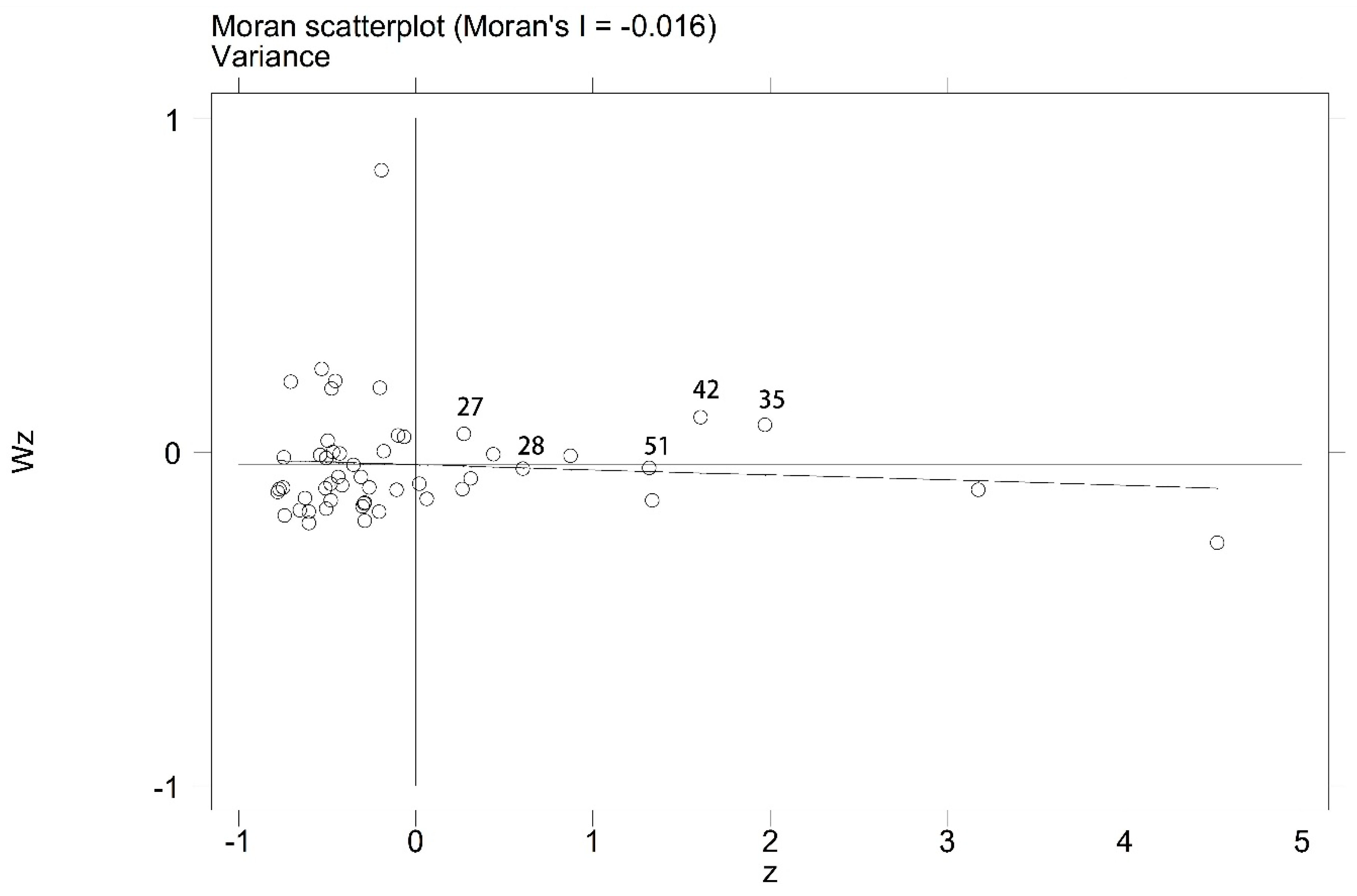
An aspect of Moran’s I the results of the global spatial autocorrelation is shown in

Table 7. Moran’s I results (measures of the global spatial autocorrelation).

Variables	I	E(I)	Sd(I)	z	p-Value
Variance	−0.016	−0.020	0.024	0.164	0.870

. The value of -0.016 with the significance of 0.870 reveals no significant spatial correlation among all the states in the statistical meaning, indicating there is no emerging regional gathering pattern in the nation, based on the variance of regional IOIS from the nation examined in our paper.

However, the local spatial autocorrelation results, as shown in

Table 8. Moran’s I results (measures of the local spatial autocorrelation).

No.	Location	Ii	E(Ii)	sd(Ii)	z	p-Value *
1	Alabama	0.130	−0.020	0.121	1.231	0.218
2	Alaska	−0.010	−0.020	0.077	0.127	0.899
3	Arizona	0.005	−0.020	0.093	0.265	0.791
4	Arkansas	0.037	−0.020	0.101	0.561	0.574
5	California	−0.135	−0.020	0.201	−0.573	0.567
6	Colorado	−0.092	−0.020	0.151	−0.479	0.632
7	Connecticut	0.043	−0.020	0.187	0.334	0.738
8	Delaware	−0.098	−0.020	0.190	−0.415	0.678
9	DC	−1.251	−0.020	0.245	−5.015	0.000 **
10	Florida	0.110	−0.020	0.113	1.151	0.250
11	Georgia	0.144	−0.020	0.118	1.389	0.165
12	Hawaii	−0.004	−0.020	0.069	0.233	0.816
13	Idaho	−0.003	−0.020	0.120	0.138	0.890
14	Illinois	0.096	−0.020	0.109	1.056	0.291
15	Indiana	0.044	−0.020	0.117	0.549	0.583
16	Iowa	−0.025	−0.020	0.113	−0.049	0.961
17	Kansas	0.014	−0.020	0.119	0.281	0.779
18	Kentucky	0.071	−0.020	0.119	0.764	0.445
19	Louisiana	0.088	−0.020	0.121	0.890	0.374
20	Maine	0.029	−0.020	0.163	0.296	0.767
21	Maryland	−0.165	−0.020	0.249	−0.583	0.560
22	Massachusetts	0.050	−0.020	0.233	0.299	0.765
23	Michigan	−0.030	−0.020	0.099	−0.105	0.917
24	Minnesota	−0.017	−0.020	0.100	0.028	0.977
25	Mississippi	0.061	−0.020	0.120	0.666	0.506
26	Missouri	0.088	−0.020	0.110	0.980	0.327
27	Montana	0.015	−0.020	0.103	0.337	0.736
28	Nebraska	−0.031	−0.020	0.121	−0.093	0.926
29	Nevada	−0.198	−0.020	0.192	−0.928	0.353
30	New Hampshire	0.056	−0.020	0.199	0.382	0.703
31	New Jersey	−0.000	−0.020	0.157	0.123	0.902
32	New Mexico	0.009	−0.020	0.097	0.299	0.765
33	New York	0.012	−0.020	0.165	0.194	0.846
34	North Carolina	0.012	−0.020	0.121	0.264	0.792
35	North Dakota	0.161	−0.020	0.110	1.644	0.100 **
36	Ohio	0.034	−0.020	0.118	0.454	0.650
37	Oklahoma	0.046	−0.020	0.095	0.692	0.489
38	Oregon	0.002	−0.020	0.163	0.131	0.896
39	Pennsylvania	−0.151	−0.020	0.157	−0.834	0.404
40	Rhode Island	0.046	−0.020	0.229	0.285	0.775
41	South Carolina	0.089	−0.020	0.110	0.983	0.326
42	South Dakota	0.170	−0.020	0.111	1.713	0.087 **
43	Tennessee	0.117	−0.020	0.105	1.300	0.194
44	Texas	0.081	−0.020	0.089	1.131	0.258
45	Utah	−0.005	−0.020	0.107	0.138	0.890
46	Vermont	−0.009	−0.020	0.169	0.063	0.950
47	Virginia	−0.040	−0.020	0.148	−0.135	0.893
48	Washington	0.000	−0.020	0.163	0.121	0.904
49	West Virginia	−0.002	−0.020	0.115	0.152	0.879
50	Wisconsin	0.023	−0.020	0.102	0.420	0.675
51	Wyoming	−0.066	−0.020	0.150	−0.305	0.760
52	Puerto Rico	−0.365	−0.020	0.072	−4.799	0.000 **

* 2-tail test, ** with an obvious statistical significance.

, provide us with some clues to grasp some regional clustering features based on the variance values examined in our paper. Some states are spatially correlated with a p-value lower than 0.1, indicating a statistical significance. The Moran’s I value of South Dakoda and North Dakoda are positive, indicating these two states have a trend of clustering spatially based on the IOIS variance from the nation. Combining the illustration of the scatterplot in Figure 1 we can get a clearer view of the spatial clustering trend of the variance values. According to Moran’s I definition of the spatial autocorrelation, the points in the first quadrant present some states with relatively high Moran’s I values clustering together spatially. Specifically, around South Dakoda and North Dakoda there exist Wyoming, Montana and Nebraska. These points representing the five states are all in the first quadrant (as numbered in the figure), and they are indeed close and adjacent to each other in the real spatial layout. Other states with statistical significance involve DC and Puerto Rico. They are in the fourth quadrant, indicating there emerges differentiated and dispersed spatial trend around these two states. Because no clear spatial correlations in real meaning are visible about these two states, we will not conduct detailed analysis in this particular paper.

Besides the regional clustering feature with a statistical significance obtained from Moran’s I analysis, we can also get a more direct sense of the regional appearance of IOIS from the map. Figure 2 shows the integrated occupational and industrial structural variant results in three by three digits. The map reveals some regional similarities in the amount of overall variance between each state and the national averages for the industry/occupation pairs. The southeastern US generally has smaller variance as do parts of the Midwest/rust belt and the southwest, including California; while the northern prairie states have industry/occupation distributions that are most different to the US averages. Some of the most populous US states (California, Texas, Illinois, Arizona, Florida, Georgia, Missouri) have a smaller variation with the US average. However, some of the more populated states (New York, New Jersey, Ohio, Virginia, Colorado, Michigan) show relatively higher variation with the US. Overall, the map shows that while there are some regional US patterns, some states still show individual variation.

5. Conclusions with Policy Implications and Further Work

The focus on the occupational mix in the regions and cities is nothing new. Researchers and planning practitioners have been making endeavors to integrate the occupational factor in economic development for the last several decades. The increasingly close linkages with the industrial analysis framework make occupations no longer just part of labor incentive research. The occupational analysis is supposed to be released out of the package and used broadly in the economic decision-making and agenda. The previous work in this field has done a lot to show the industrial and occupational analysis could not substitute each other. The gap and differences do, in fact, exist. Neither aspect will be neglected in effective planning practice. This paper constructs an integrated occupational and industrial structure (IOIS) to bind them together. It will lead to some policy implications in potential regional economic and human capital policy-making. Firstly, in regional perspective, the new integrated analytical approach will provide a more comprehensive and different view about the regional and national development situations. The state of California serves as the data source of the comparison between the integrated and single applied approach. It does demonstrate that the integrated approach reveals a bigger difference between the state and national level because the identified variance values increase when using the integrated approach. As a new perspective and method, it will serve as protentional policy information tools for the regional policy-making. It will better recognize the regional advantage and competitiveness compared with the national situation as a whole. Regions can gain an advantageous position by targeting more precisely in the development fields. This integrated framework provides a different option either in theoretical research or in practical plans. The occupation included a framework of the regional economy is of greater importance to the states which have an abundant human resource and creative talents, such as California. The single industrial analysis only provides the relatively fixed structure of the regional economy. And the single occupational analysis gives the limited information of the human resource pool. But the integrated framework tells us which kind of human resource is “alive” in the practical use corresponding to a certain industry. It helps the policy-makers bridge the industry requirement with the occupational supply by giving deeper insight into the regional development.

Secondly, in a national perspective, it is applied in the 52 state data files in PUMS. The overview of the national industrial and occupational status is provided. The snapshot shows most of the states have a highly similar occupational and industrial development with the national level. The occupations and industries are distributed relatively evenly across the nation. It needs further and detailed analysis in specific industries and areas to identify more potential benefits. In some sense, the results reflect that occupations play an even more important role in the industrial structure. An adjustment, made by gradually more detailed data level in terms of either occupations or industries, reveals that focusing more on occupational mix helps the state IOIS become more differentiated from the national level, while the industrial framework does less. The value change range is even bigger in the occupational aspect compared with the industrial one. It goes further to suggest the occupational aspect and human resources play an important role in achieving a unique regional advantage across the nation. From the variance results of the states, we learn that some states (such as Florida, Hawaii, Indiana, Michigan, Nevada) are not sensitive to the changes of more detailed occupational information. For example, their variance values even decrease when the I3O2 change to I3O3, indicating they grow more similar to the national average level. It might be an indication that under certain industrial frame, the human resource is in a disadvantageous position. In comparison, some states (such as California, Illinois, Maryland, to just name a few) have variance values increase from I3O2 to I3O3. These states have more available human capital potential. From the national point of view, it will help the policy makers mobilize the human resource and formulate labor incentive policies in a larger range more effectively.

The integrated industrial and occupational approach provided in this paper is just a start. Upcoming research shall be in more detailed and specific industrial and occupational groups to help with the policy-making of the urban and regional development. Because the occupational and human capital focus is mostly related to the industries containing the most knowledge and skill-intensified contents, the future research shall involve more efforts in the creative and knowledge industrial groups with the generalized ISIO approach. Of course, the creative industries refer to the broad sense, including design, software developing, art, performing, consulting and so on., all of which are of great significance to upgrade the industrial development and refuel the regional growth.

References

- Thompson, W.R.; Thompson, P.R. From industries to occupations: Rethinking local economic development. Econ. Dev. Comment. 1985, 9, 12–18. [Google Scholar]
- Thompson, W.R.; Thompson, P.R. National Industries and Local Occupational Strengths: The Cross-Hairs of Targeting. Urban. Stud. 1987, 24, 547–560. [Google Scholar] [CrossRef]
- Marshall, A. Principles of Economics, 8th ed.; Macmillan: London, UK, 1890. [Google Scholar]
- Ohlin, B. Interregional and International Trade; Harvard University Press: Cambridge, MA, USA, 1933. [Google Scholar]
- North, D.C. Location Theory and Regional Economic Growth. J. Polit Econ. 1955, 63, 243–258. [Google Scholar] [CrossRef]
- Tiebout, C.M. Exports and Regional Economic Growth. J. Polit. Econ. 1956, 64, 160–164. [Google Scholar] [CrossRef]
- Isard, W. Location and Space-Economy: A General Theory Relating to Industrial Location, Market Areas, Land Use, Trade, and Urban Structure; Technology Press of Massachusetts Institute of Technology and Wiley: Cambridge, MA, USA, 1956. [Google Scholar]
- Balassa, B. Trade Liberalization among Industrial Countries: Objectives and Alternatives; McGraw-Hill: New York, NY, USA, 1967. [Google Scholar]
- Krugman, P. Increasing returns, monopolistic competition and international trade. J. Int. Econ. 1979, 9, 469–479. [Google Scholar] [CrossRef]
- Hummels, D.; Klenow, P. The variety and quality of a nation’s exports. Am. Econ. Rev. 2005, 95, 704–723. [Google Scholar] [CrossRef]
- Helpman, E. Trade, FDI and the organization of firms. J. Econ. Lit. 2006, 44, 589–630. [Google Scholar] [CrossRef]
- Schumpeter, J. The process of creative destruction. In Capitalism, Socialism and Democracy; Harper & Brothers: New York, NY, USA, 1942; pp. 81–86. [Google Scholar]
- Jacobs, J. The Economy of Cities; Random House: New York, NY, USA, 1969. [Google Scholar]
- Piore, M.J.; Sabel, C.F. The Second Industrial Divide: Possibilities for Prosperity; Basic Books: New York, NY, USA, 1984. [Google Scholar]
- Lucas, R.E. On the mechanics of economic development. J. Monet. Econ. 1988, 22, 3–42. [Google Scholar] [CrossRef]
- Drucker, P. Post-Capitalist Society; Harper Business: New York, NY, USA, 1993. [Google Scholar]
- Saxenian, A. Regional Advantage: Culture and Competition in Silicon Valley and Route 128; Harvard University Press: Cambridge, MA, USA, 1994. [Google Scholar]
- Audretsch, D.B.; Feldman, M.P. Knowledge spillovers and the geography of innovation and production. Am. Econ. Rev. 1996, 86, 630–640. [Google Scholar]
- Storper, M. The Regional World: Territorial Development in a Global Economy; The Guilford Press: New York, NY, USA, 1997. [Google Scholar]
- Porter, M. Clusters and the new economics of competition. Harv. Bus. Rev. 1998, 76, 77–90. [Google Scholar]
- Florida, R. The Rise of the Creative Class; Basic Books: New York, NY, USA, 2002. [Google Scholar]
- Glaeser, E. The Rise of the Skilled City; Working Paper No. 10191; National Bureau of Economic Research, Harvard University: Cambridge, MA, USA, 2003. [Google Scholar]
- Stolarick, K.; Florida, R. Creativity, Connections and Innovation: A Study of Linkages in the Montréal Region. Environ. Plan. A Econ. Space 2006, 38, 1799–1817. [Google Scholar] [CrossRef]
- Scott, A.J. Space-Time Variations of Human Capital Assets Across U.S. Metropolitan Areas 1980–2000. Econ. Geogr. 2010, 86, 233–249. [Google Scholar] [CrossRef] [PubMed]
- Berry, C.R.; Glaeser, E.L. The divergence of human capital levels across cities. Pap. Reg. Sci. 2005, 84, 407–444. [Google Scholar] [CrossRef]
- Rauch, J.E. Productivity Gains from Geographic Concentration of Human Capital: Evidence from the Cities. J. Urban. Econ. 1993, 34, 380–400. [Google Scholar] [CrossRef] [Green Version]
- Wheeler, C.H. Do localization economies derive from human capital externalities? Ann. Reg. Sci. 2007, 41, 31–50. [Google Scholar] [CrossRef]
- Balfe, K.P.; McDonald, J.F. Emerging Employment Opportunities and Implications for Training; NCI Research: Evanston, IL, USA, 1994. [Google Scholar]
- Feser, E.J. What Regions Do Rather than Make: A Proposed Set of Knowledge-based Occupation Clusters. Urban. Stud. 2003, 40, 1937–1958. [Google Scholar] [CrossRef]
- Markusen, A. Longer view: Targeting occupations in regional and community economic development. J. Am. Plan. Assoc. 2004, 70, 253–268. [Google Scholar] [CrossRef]
- Barbour, E.; Markusen, A. Regional occupational and industrial structure: Does one imply the other? Int. Reg. Sci. Rev. 2007, 30, 72–90. [Google Scholar] [CrossRef]
- Currid, E.; Stolarick, K. The occupation-Industry Mismatch: New Trajectories for Regional Cluster Analysis and Economic development. Urban Stud. 2010, 42, 337–362. [Google Scholar] [CrossRef]
- Nolan, C.; Morrison, E.; Kumar, I.; Galloway, H.; Cordes, S. Liking Industry and Occupation Clusters in Regional Economic Development. Econ. Dev. Q. 2011, 25, 26–35. [Google Scholar] [CrossRef]
- Bacolod, M.; Blum, B.S.; Strange, W.C. Urban interactions: Soft skills versus specialization. J. Econ. Geogr. 2009, 9, 227–262. [Google Scholar] [CrossRef]
- Florida, R.; Mellander, C.; Stolarick, K.; Ross, A. Cities, skills and wages. J. Econ. Geogr. 2012, 12, 355–377. [Google Scholar] [CrossRef]
- Gabe, T.M.; Abel, J.R. Specialized knowledge and the geographic concentration of occupations. J. Econ. Geogr. 2012, 12, 435–453. [Google Scholar] [CrossRef]
- Mellander, C. Creative and Knowledge Industries: An Occupational Distribution Approach. Econ. Dev. Q. 2009, 23, 294–305. [Google Scholar] [CrossRef]
Figure 1.
Scatterplot based on the variance values.
Figure 2.
US States Industry/Occupation Variance by State.