Enterprise Resilience Assessment—A Quantitative Approach

Abstract

Enterprise resilience is a key capacity to guarantee enterprises’ long-term continuity. This paper proposes a quantitative approach to enhance enterprise resilience by selecting optimal preventive actions to be activated to cushion the impact of disruptive events and to improve preparedness capability, one of the pillars of the enterprise resilience capacity. The proposed algorithms combine the dynamic programming approach with attenuation formulas to model real improvements when a combined set of preventive actions is activated for the same disruptive event. A numerical example is presented that shows remarkable reductions in the expected annual cost due to potential disruptive events.

1. Introduction

Every year, both natural and manmade disasters impact the economies of countries all over the world [1]. Enterprises lack a risk culture and they are exposed to a very dynamic environment filled with threats and disruptive events that endanger the continuity of their business [2].

Events like air travel disruptions after the 2010 Eyjafjallajökull eruption in Iceland affected many enterprises since the controlled air space of several European countries was closed, and the transport of components and goods was also interrupted. This had a very negative impact on enterprises as they did not know if goods would arrive on time.

Several authors have analyzed the impact of different disruptive events that have occurred in recent years. Sheffi and Rice [3] explain that after the September 11 terrorist attacks in 2001, the US government closed the country’s borders and shut down all incoming and outgoing flights, and how this event affected enterprises worldwide. Another example explains how Nokia and Ericsson, both regular customers of Philips, responded to a fire at Philips Alburquerque’s industrial facility. Both companies recovered from this disruptive event in a very different manner. While Nokia started to search for alternatives to replenish the chips that Philips supplied them, Ericsson assumed that chips would be delivered with some delay. However, Philips needed more time than it initially expected to restart its production. Based on this example, Nokia responded in a more efficient way to such a disruptive event, thus Nokia was more resilient [4].

Moreover, the current organizational environment characterized by a high degree of information sharing, an increasing complexity of transactions among supply chain partners [5,6], the fierce competition, the bargaining power of clients, the dependence on suppliers, the constant demand for innovation, changes in the regulatory environment, the new expectations of society [7], the constitutional changes such as UK’s planned exit from the European Union (Brexit) [8] make enterprises more vulnerable and consequently, companies should enhance their resilient capacity to efficiently manage this complexity. Prior and Hagmann [9] state that today, a significant challenge, lies in the accurate characterization and quantification of resilience.

Dalziell and McManus [10] suggest that resilience was firstly proposed in the field of ecology by Holling [11], who stated that resilience is how a system behaves when it is in equilibrium, and it is stressed and moved from this stability. In other words, it is a system’s ability to withstand a major disruption within acceptable degradation parameters, and to recover in an acceptable time and with composite costs and risks [12].

Doorn [13] performed an analysis that shows that different disciplines employ various definitions of resilience and conceptions of its relation to vulnerability. Erol et al. [14] define enterprise resilience (ER) as the capacity to lower the level of vulnerability to expected and unexpected disruptions, its ability to change itself and to adapt to its changing environment, and its ability to recover in the shortest possible time. Scholz et al. [15] state that resilience incorporates the capability of a system to cope with the adverse effects that a system has been exposed to and distinguish between specified (known events) and general resilience (unknown events). Hollnagel [16] defines resilience as a system’s capacity to prevent, recognize, anticipate and react to risks before their adverse consequences take place. Levalle and Nof [17] focuses the attention on supply chains and defines resilience as the inherent ability of a supply network agent and/or the emergent capability of a supply network to (i) anticipate errors and conflicts, (ii) prevent them from creating disruptions to normal operation, and (iii) overcome disruptions with minimum quality of service loss, within sustainable use of resources. In light of this, Kamalahmadi and Parast [18] consider three phases for supply chain resilience, which are (i) anticipation; (ii) resistance; and (iii) recovery and responses. In the same line, Ponomarov and Holcomb [19] identify readiness, response, and recovery, as the main necessary capacities to build resilient organizations. Takin into account that resilience is a multidisciplinary and multifaceted concept, its enhancement requires efficient strategies to deal with and manage disruptive events.

Most authors state that one of the main and more successful strategies is to prevent and be prepared for the unexpected in advance [17,18,19,20,21,22]. Wildavsky [23] proposed creating a balance of anticipation and resilience as a strategy to reduce risks under uncertain conditions. As Ayyub [24] states, enhancing resilience could lead to massive savings through reducing risks. In this case, it is assumed essential to be prepared to anticipate the negative effects of an event. Resilient companies are proactive, and thanks to their preparation and anticipation capacities, they are able to recover better from difficulties [25]. Chesley and Amitrano [20] define ER as the capacity to be ready and prepared to face up to disruptions, so that all the importance is attributed to the preparedness capacity. However, companies often spend too little on prevention or mitigation, and too much on reaction [26]. Schmitt and Singh [27] explains that increasing a firm’s supply chain resilience is largely dependent on what options an organization has to react as a system if a disruption occurs, and on how much safety is built into the system (through inventory reserves, redundant suppliers, etc.), that is through the implementation of preventive actions that are part of the enterprises’ preparedness capacity. Dabhilkar et al. [28] declares that resilience capabilities are conceptualized along two dichotomous dimensions “proactive/reactive” and “internal/external”.

Notwithstanding, it is unquestionable that ER capacity relies on the proactive perspective through the preparedness capability. Nevertheless, how can an enterprise be prepared for unexpected events? The response to this question is uncertain because it is impossible to be fully prepared for unforeseen events. However, enterprises should improve their preparedness capacity by implementing certain preventive actions, where prevention is key to be prepared for disruptive events, and to thus be more resilient.

ER is not only a function of the preparedness capacity to react to disruptive events in a proactive way, but it also depends on the adaptive capacity [29] and the recovery ability to adjust to and recover from such disruptive events. However, assessing the adaptative and recovery capacities is beyond the scope of this research.

Research on resilience has proliferated in recent years. Numerous definitions, tactics, metrics, and indices have been proposed. However, most of them are formulations with little or no formalized theoretical underpinnings [30]. Polyviou et al. [31] state that firms of all sizes are concerned with avoiding or recovering quickly from disruptions. For this reason, the authors point out that researchers have to respond to this emerging concern and develop frameworks and tools that advance theory and practice in the area of firm and supply chain resilience.

Consequently, the main objective of this paper is to analyze how to cushion the effects of potential disruptive events on an enterprise by implementing preventive actions based on the dynamic programming foundations. This article explains how to (which actions should be implemented) enhance the preparedness capability in order to build resilient enterprises. An analysis of what preventive actions for each disruptive event should be implemented is performed by a dynamic programming approach to solve the problem.

The paper is organized as follows. Section 2 defines a specific problem related to lack of preparedness capability to face production problems and describes the dynamic programming approach used to solve this quantitative problem. Moreover, it presents the special features of the problem characterization when a combined set of preventive actions on the same disruptive event is activated, along with our proposal to deal with this issue and the problem modeling. Section 3 shows and discusses the results of which preventive actions are to be activated to improve the preparedness capability using the dynamic programming approach and summarizes future research lines to improve the resilient capacity of enterprises. Finally, Section 4 offers the main conclusions.

2. Materials and Methods

2.1. Problem Definition

ER relies on the preparedness capability to deal with disruptive events. In order to assess the ER capacity, Sanchis and Poler [32] developed a framework to categorize disruptions. Within this framework, a disruptive event is considered a foreseeable or unforeseeable event that directly affects an enterprise’s usual operation and its stability [33]. Disruptive events are classified into different categories depending on the source from which they originated; e.g., accidental, customer, energy, equipment, financial, technology, infrastructure, man-made, natural, political, product, regulatory, supplier and terrorism. The problem addressed in this study belongs to the “productions” category.

An exhaustive literature review was done to identify the commonest disruptive events related to the production category. The literature review focused mainly on two types of information sources: on the one hand, reports prepared by leading consulting firms, such as Ernst & Young, and specialized entities in risk and ER, such as the Business Continuity Institute, which develops annual reports with rankings of the situations or risks that most concern the business world [34,35,36,37,38,39,40]; on the other hand, scientific publications were also reviewed to find the most frequent and worrisome disruptive events related to production aspects [41,42,43].

Disruptive events, such as damage to machinery/equipment, failure to produce innovative products to satisfy customer needs, disruptive manufacturing technologies/innovation, product quality incident, outage, inaccurate manufacturing planning, among others, were found to be relevant and worrisome events for the business world. In order to test the proposed method, the example problem was simplified by considering only four disruptive events related to potential production problems: (i) Limiting changes in the production capacity; (ii) Breakdown/failure of machines or key equipment; (iii) Production operations that become increasingly complex; and (iv) Production of defective or poor quality products.

Some preventive actions were proposed for all the previous disruptive events. The validation of the suitability and appropriateness of these preventive actions was analyzed by a panel of experts in an iterative process through a Delphi study. After the formulation of the problem (to validate the set of preventive actions proposed for each disruptive event) and the choice of experts, a questionnaire was developed and launched. The questionnaire had a 3-point Likert scale, where experts had to indicate the interest of each of the preventive action proposed (high, medium or low interest) per disruptive event. Moreover, the experts were also invited to add other interesting preventive actions and through an iterative process consisted of two rounds, the most significative ones were selected. The 12 experts who participated in the Delphi study came from research, academia and business/industrial areas from different knowledge domains related to resilience. More information could be found in Sanchis and Poler [44].

All in all, the problem consisted in four potential disruptive events that could occur, plus the proposal of different preventive actions per disruptive event (validated by the Delphi study) to minimize impacts (in terms of the expected annual cost). It is worth mentioning that in this example, the disruptive events are internally originated in the enterprise. However, the potential disruptive events could happen in the supply chain where the enterprise operates or even externally to this supply chain. With regards to the preventive actions, some are also internally managed by the enterprise, but others involve entities of its supply chain.

Table 1. Example of the problem definition: disruptive events analyzed and the proposal of preventive actions.

Disruptive Event	Preventive Actions
P1: Limiting changes in the production capacity	P1.1: Implementation of demand forecasting systems.
	P1.2: Introduction of strategies for reducing setting-up times (Single-Minute Exchange of Die—SMED).
	P1.3: Introduction of advanced predictive maintenance systems to increase the availability of production resources.
P2: Breakdown/failure of machines or key equipment	P2.1: Total preventive maintenance.
	P2.2: Negotiation with competitors (orders to competitors).
	P2.3: Backward vertical integration of the technical service.
P3: Production operations that become increasingly complex	P3.1: Rationalization of the products’ offerings reviewing the design concept and development of new products.
	P3.2: Implementation of approaches/strategies (modularization, postponement) for manufacturing and assembly processes.
	P3.3: Implementation of advanced technologies for production planning and control.
P4: Production of defective or poor-quality products	P4.1: Supplier qualification: inspection and testing of raw materials.
	P4.2: System for quality assurance.
	P4.3: General training for quality.

shows the four analyzed disruptive events and the proposal of preventive actions.

Quantifying the impact of the potential disruptive events is modeled by the expected annual cost of each disruptive event k (Cd_k), the annual cost of the preventive action n (i_n), the expected annual cost of a disruptive event k after activating a preventive action n (Cdp_k), the savings of a disruptive event after implementing a preventive action n (a_n) and the annual investment in ER (Inv).

2.2. Dynamic Programming: The Knapsack Approach

The term dynamic programming was originally coined by Richard Bellman in the 1940s to define the problem-solving process in which each problem depended on and necessitated the solution of another problem. The Bellman equation provides modeling according to a recursive relation [45,46].

Due to the synergies that the problem defined in Section 2.1 presents with capital budgeting problems, the literature review which focused on this area revealed that the major contributions and the fundamental primary studies related to dynamic programming and capital allocation were performed by these authors in the 1960s [47,48,49,50].

The basic capital allocation problem considers a firm that has various investment proposals, called projects, each of which requires capital outlays and yielded returns [51]. To solve such problems, the most widely used approach is dynamic programming, specifically the knapsack approach. However, real problems usually entail greater complexity than the basic capital allocation problem. Weingartner [48] stated that the dynamic programming approach has its limitations, such as dependency among projects when a specific project is developed, and it depends on the development of another project or more. As in the dynamic programming solution to the knapsack problem, the time sequence is replaced with the sequence of projects being considered, but the ordering of the projects to be implemented is arbitrary.

Currently, different studies have based their research on previous works, and the present research lines are addressed to solve multidimensional knapsack problems, which combine dynamic programming and branch and bound [51].

The decision problem proposed herein is NP-complete. The literature reveals that dynamic programming algorithms are the most suitable type to solve such optimization problems. Their simplicity, flexibility and rapidness make the dynamic programming approach a powerful solving method. Bhowmik [52] states that it is so powerful that it encourages tremendous growth in research works for solving decision problems. Dynamic programming research has made fundamental advances in theory, numerical methods and econometrics. Thus, dynamic programming can be viewed as a useful “first approach” scheme to human decision making.

The knapsack method appears in real-world decision-making processes in a wide variety of fields. Skiena [53] shows that among 75 algorithmic problems, the knapsack problem was the 18th most widely used and the 4th most needed to solve real problems. In the knapsack problem, a container has a certain capacity, and each item that can go into the container has a size and a benefit. The problem lies in determining what should go into the container to maximize the total benefit.

In the case presented in this paper in Section 2.1, capacity is related to the investment that the enterprise is willing to make to improve its ER capacity. Items are the different preventive actions that could be activated to reduce the expected annual cost of disruptive events. Size is the cost of each preventive action and profit is the savings that the enterprise notices after implementing the preventive actions. In this case and based on the definition of the general knapsack problem goal, the enterprise’s objective is to maximize total savings.

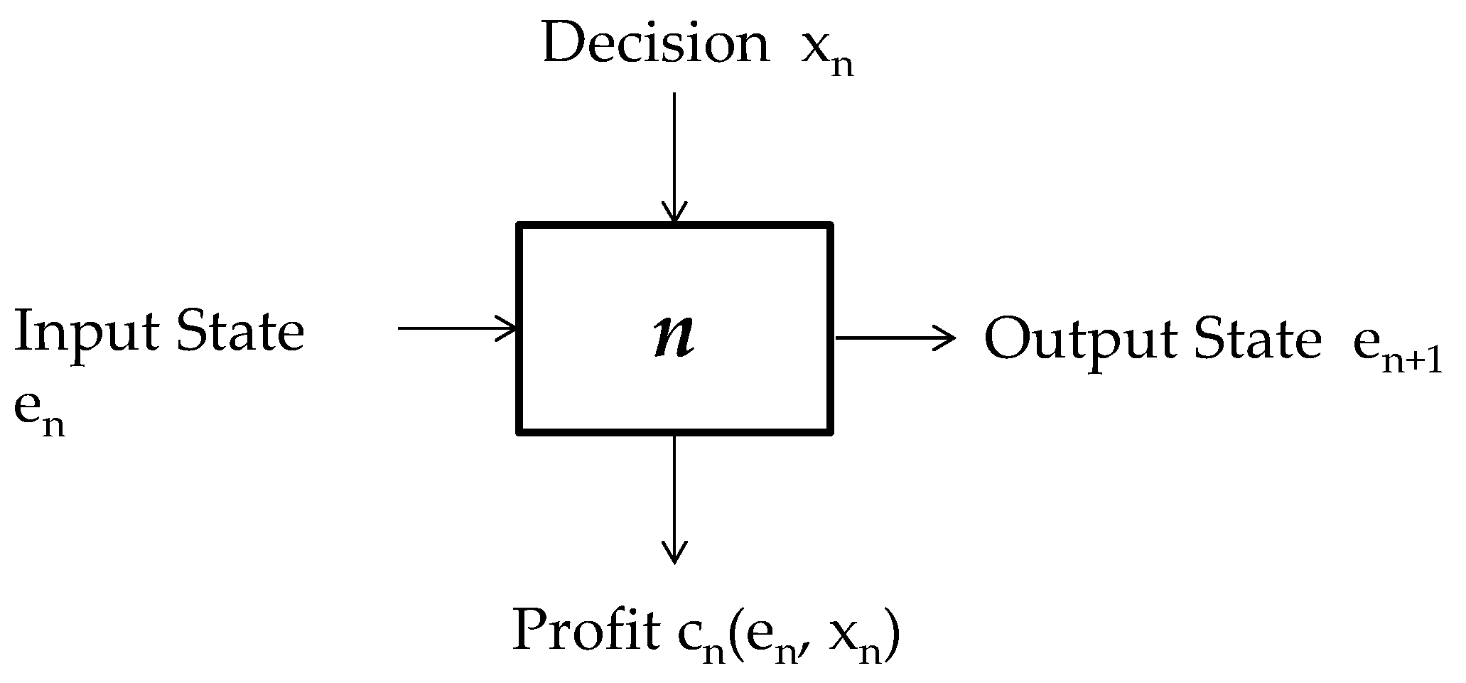
A dynamic programming problem can be divided into different decision stages. Each stage has an input state (e_n) and, depending on the decision made (x_n), an output state (e_n+1) is obtained. This output state generates a profit (c_n), which depends on both the decision and input state (see Figure 1).

Table 2. Nomenclature of dynamic programming knapsack problems.

Nomenclature	General Description	Problem Description
N	Number of stages	Number of preventive actions
xn	Decision in stage n	Decision about activating the preventive action n (1: activated; 0: otherwise).
en	Input state	Enterprise Resilience (ER) investment (Inv) available before deciding about activating preventive action n.
cn(en,xn)	Profit in stage n	Saving made by activating (xn = 1) preventive action n: xn·an
in	Unitary cost	Cost of activating preventive action n
an	Unitary profit	Unitary savings from the disruptive events affected by preventive action n.
fn(en,xn)	Total profit accumulated from stage n to stage N	Total savings accumulated from activating the strategy of the preventive actions from stage n to stage N
xn *	Optimal decision	The best activation strategy for the preventive actions from stage n to stage N.
fn* (en)	Total optimum in stage n (with xn *)	Total optimum saving of the best activation strategy for the preventive actions from stage n to stage N given an input state en.
fn (en, xn) = f * n+1(en+1) + vn·xn	Recursive relation	Total saving made with an activation strategy for the preventive actions from stage n to stage N given an input state en and taking the decision xn.
en+1= en − in·xn	The following input state	ER investment available after deciding about activating preventive action n. The following input state is equal to the investment available before minus preventive action n activated (if xn = 1), multiplied by its unitary cost (in).

The optimal profits in each stage, as well as the optimal decisions, are calculated as follows: fn * (e_n) = opt {c_n(e_n,x_n) ⊗... ⊗ c₁(e₁,x₁)}: total optimal profit in stage n (with x *).

shows the common nomenclature used in the proposed dynamic programming model, a general description from a knapsack problem point of view and the description of the decision problem defined in Section 2.1.

2.3. Special Features in Activating Preventive Actions

The problem defined in Section 2.1 presents special features as to the activation of a combined set of preventive actions that affect the same disruptive event. When this occurs, improvements in savings terms are not necessarily the sum of the savings provided by all the activated preventive actions. This characteristic presents synergies with the pharmacology science studies of Chou et al., which focus on analyzing combined drug effects [54,55]. Belen’kii and Schinazi [56] analyze the antagonism, synergy or additivism for drug combinations. From these concepts, antagonism is in line with the present study. Antagonism (or depotentiation, negative interaction, negative synergy, etc.) is defined as the joint effect of two drugs or more, in such a way that the combined effect is less than the sum of the effects produced by each agent separately [57,58].

The ER capacity enhancement problem presents a kind of antagonism in that the joint savings from the different preventive actions activated to mitigate the effects of the same disruptive event are less than the sum of all the preventive actions savings that address such a disruptive event.

In order to overcome this issue and based on the fact that enterprises are those that provide the information about disruptive events, preventive actions, costs and savings, one of the alternatives would be to ask the enterprise for this piece of information. The enterprise should provide data about the savings that some preventive actions generate when activated in an isolated manner for a specific disruptive event.

Moreover, the enterprise should provide data on the savings generated when different combinations of such preventive actions are activated for the same disruptive event. However, this exercise is very complex and exhausting for enterprises, and the information they provide might not be truthful. In order to overcome this, and by considering that the savings effect of multiple preventive actions on the same disruptive event is less than its sum, an attenuation formula is proposed.

This formula (1) slows down savings when two preventive actions or more on the same disruptive event are activated in the optimal solution by calculating an attenuation parameter:

$${\mu }_n=\mathsf{\alpha }·\frac{ln\left(n\_ac{t}_k\right)}{n\_ac{t}_k-1}$$

(1)

where, α: Parameter related to the magnitude of the attenuation (0 ≤ α ≤1). n_act_k: Number of preventative actions activated in the optimal solution for the same disruptive event.

The proposed attenuation parameter follows logarithmic reduction, which is based on different studies that have focused on analyzing the effects of a drugs combination from other diverse research areas; e.g., pharmacology, medicine, etc. [59,60]. The definition of value α depends on the degree that enterprises wish to be attenuated when multiple preventive actions are activated for the same disruptive event. It is worth mentioning that the higher parameter α, the less marked the attenuation becomes.

Among the preventive actions activated for the same disruptive event, the preventive action with the highest saving is not attenuated because, although several preventive actions are activated, it is presumed that the savings of the disruptive event is, at least, the maximum saving of all the preventive actions activated. Therefore, the attenuation parameter is applied only to those savings that are lower than the maximum, as it can be seen in the description of Algorithm 1.

Algorithm 1. Attenuation of preventive actions n activated for the same disruptive event k

at = false

fork in {K}

for n in {Ni}

if mkn= false

if akn < Max{ak}

akn = akn · μn

mkn = true

at = true

enfif

endif

endfor

endfor

Algorithm 1 calculates for all the disruptive events (K) and for all the preventive actions activated (N_i), if such preventive actions have not been attenuated in previous iterations (m_kn = false). It also calculates which savings are lower than the maximum saving per disruptive event, which is attenuated by the proposed parameter μ_n, while the status of the attenuated preventive actions is set to true (m_kn = true). The algorithm also registers if any attenuation has been performed (at least one preventive action has been attenuated) and establishes that a_t is also set to true.

The Algorithm 2 is the main algorithm loop that launches dynamic programming optimization and the attenuation. The loop ends when no attenuation is performed.

Algorithm 2. The main algorithm loop

at = true

whileat = true

Solve by Dynamic Programming

Apply Attenuation

endwhile

2.4. Problem Modeling

The problem presented in Section 2.1 was quantified with realistic data to show a calculation example.

Table 3. Problem data definition (€ thousands).

Code	Disruptive Event	Cdk	#	Preventive Actions	in	Cdpk	an
P1	Limiting changes in the production capacity	10,000	P1.1	Implementation of demand forecasting systems.	2000	6000	4000
			P1.2	Introduction of strategies for reducing setting-up times (SMED…).	1000	7000	3000
			P1.3	Introduction of advanced predictive maintenance systems to increase the availability of production resources.	1000	8000	2000
P2	Breakdown/failure of machines or key equipment	25,000	P2.1	Total preventive maintenance.	3000	18,000	7000
			P2.2	Negotiation with competitors (orders to competitors).	2000	20,000	5000
			P2.3	Backward vertical integration of the technical service.	5000	17,000	8000
P3	Production operations that become increasingly complex	15,000	P3.1	Rationalization of the products’ offerings reviewing the design concept and development of new products.	1000	13,000	2000
			P3.2	Implementation of approaches/strategies (modularization, postponement) for manufacturing and assembly processes.	2000	10,000	5000
			P3.3	Implementation of advanced technologies for production planning and control.	5000	3000	12,000
P4	Production of defective or poor-quality products	40,000	P4.1	Supplier qualification: inspection and testing of raw materials.	2000	30,000	10,000
			P4.2	System for quality assurance.	8000	23,000	17,000
			P4.3	General training for quality.	1000	37,000	3000

shows the quantification for parameters Cd_k, i_n, Cdp_k and a_n after taking into account that the savings of a disruptive event k after implementing a preventive action n are defined by Equation (2):

$$a_n=C{d}_k-Cd{p}_k$$

(2)

By way of example, for disruptive event “P1: Limiting changes in the capacity of production”, the expected annual cost is €10,000. However, the enterprise could implement three different preventive actions to be better prepared to face the negative effects of this event when it occurs and, in turn, to be more resilient. These preventive actions are P1.1, P1.2 and P1.3 (described in Table 3). The enterprise estimates that preventive action P1.1 has an annual cost of €2000, and the expected annual cost of P1 will lower to €6000 if this preventive action is finally activated. Therefore, the savings (without considering the cost of the preventive action) will be the difference between the initial expected annual cost and the cost after activating the preventive action (e.g., €10,000 − €6000 = €4000), as indicated in Equation (2). This difference is because the enterprise, by activating preventive actions, has an enhanced preparedness capability to endure the negative effects of the disruptive event. Then it is assumed that the cost of the disruptive event after activating a preventive action will always be lower than before.

The cost of the preventive action should also be lower than the saving because otherwise it would be better not to activate such a preventive action, but to allow the disruptive event to occur as it is more costly to enhance preparedness capability than allowing the disruptive event to take place.

Moreover, enterprises should decide how much money they should invest to implement the most adequate preventive actions in order to enhance their ER capacity. Depending on the value of this input data, the solution of the problem will differ according to the resources used to enhance this capability. In this example, the annual investment in ER is Inv = €22,000.

Parameter α used in the attenuation process is 0.95. As shown in Table 3, the event that presents the highest expected annual cost is disruptive event P4, followed by P2. The expected annual costs of disruptive events P1 and P3 have almost the same order of magnitude. Therefore, it is expected that efforts will be made to activate preventive actions to face the negative effects of the disruptive event that presents the highest expected annual cost.

3. Results and Discussion

Three iterations are needed to compute the problem described in this paper to obtain the optimum solution, and the attenuation parameter needs to be taken into account when more than one preventive action is activated for the same disruptive event (

Table 4. The results obtained in each iteration.

Preventive Action	Iteration 1		Iteration 2		Iteration 3		Iteration 4
	xn	Return Function	xn	Return Function	xn	Return Function	xn	Return Function
P1.1	0	4000	0	4000	1	4000	1	4000
P1.2	1	3000	1	3000	1	3000	1	1975
P1.3	0	2000	1	2000	0	1317	0	1317
P2.1	0	7000	1	7000	1	7000	1	7000
P2.2	1	5000	1	5000	0	3292	0	3292
P2.3	0	8000	0	8000	0	8000	0	8000
P3.1	1	2000	0	1044	0	1044	0	1044
P3.2	1	5000	0	2609	0	2609	0	2609
P3.3	1	12,000	1	12,000	1	12,000	1	12,000
P4.1	1	10,000	1	5218	1	5218	1	5218
P4.2	1	17,000	1	17,000	1	17,000	1	17,000
P4.3	1	3000	0	1566	1	1566	1	1566

).

In the first iteration, 8 of the 12 proposed preventive actions were activated (x_n = 1), taking into account that the annual investment is respected, which was established as €22,000.

In this first iteration, as more than one preventive action was activated for each disruptive event, the attenuation parameter was applied. The return function (savings after activating preventive action n) of the attenuated preventive actions in Iteration 1 are shown in bold as the return function of Iteration 2, based on the description of Algorithm 1. In Iteration 2, seven preventive actions were activated, from which P1.3 and P2.2 were attenuated, as shown in the return function of Iteration 3. In Iteration 3, the same number of preventive actions as in the previous iterations was activated and only one preventive action (P1.2) was attenuated. Finally, in the last iteration, no. 4, the solution shows that when more than one preventive action was activated for the same disruptive event, one preventive action presented the maximum return function value (per disruptive event) and the other activated ones had already been attenuated. Therefore, Algorithm 2 ends at this point as the following iteration offers the same result as the fourth one.

The detailed results of the final solution (Iteration 4) are presented in

Table 5. The results obtained in Iteration 4 of dynamic programming.

Disruptive Event	Preventive Action	Decision (Xn)	Return Function (€)	Total Return Value (€)	Capacity Left (€)	Original Return Function (€)
P1	P1.1	1	4000	4000	20,000	4000
	P1.2	1	1975	1975	19,000	3000
	P1.3	0	1317	0	19,000	2000
P2	P2.1	1	7000	7000	16,000	7000
	P2.2	0	3292	0	16,000	5000
	P2.3	0	8000	0	16,000	8000
F3	P3.1	0	1044	0	16,000	2000
	P3.2	0	2609	0	16,000	5000
	P3.3	1	12,000	12,000	11,000	12,000
F4	P4.1	1	5218	5218	9000	10,000
	P4.2	1	17,000	17,000	1000	17,000
	P4.3	1	1566	1566	0	3000

.

In the first disruptive event, two preventive actions were activated; in disruptive events P2 and P3, only one preventive action was activated; in the “production of defective or poor quality products” disruptive event (P4), the three proposed preventive actions were activated because this was initially expected since this disruptive event presented the highest expected annual cost. Although disruptive event P4 was that in which more preventive actions were activated, it did not undergo the greatest reduction in the expected annual cost after activating the preventive actions (a reduction of almost 32%). Instead it was P3 (a reduction of 46%), followed by disruptive event P1 with an almost 40% reduction in the expected annual cost of such disruptive event after activating preventive actions P1.1 and P1.2. This could result from the fact that the preventive actions proposed for disruptive events P1 and P3 were more efficient that those proposed for disruptive event P4. Disruptive event P2 obtained the lowest savings with a 16% drop in the expected annual cost after activating preventive action P2.1.

Future research directions will be addressed to investigate how to deal with problems in which the activation of the preventive actions defined by a specific disruptive event could affect/benefit other disruptive events. In other words, a preventive action applied to a specific disruptive event could also be linked to other disruptive events. In the case proposed herein, each preventive action is unique and applies to only one disruptive event. However, further research should focus on (i) the relations between a specific preventive action and different disruptive events; and (ii) how the activation of such preventive action could affect the different disruptive events linked to it. Moreover, the proposed algorithm could be further improved to take into account the impact of (de)selecting an action on the attenuation of other actions.

Finally, further research lines aim to define an heuristic algorithm to optimally sequence and prioritize the activated preventive actions to be executed by taking into account factors such as the number of disruptive events that benefit from a preventive action activation, the impact that the activation of a preventive action has in the other disruptive events, the costs for the activation/implementation of such actions, the availability of enterprise resources over time, among others.

4. Conclusions

Enhancing the ER capacity leads to significant savings in expected annual costs by activating preventive actions that improve the preparedness capability, one of the main pillars of the ER capacity. This article shows a realistic problem in which an enterprise has to analyze four potential production problems and how different preventive actions can improve its preparedness and, in turn, its ER capacity. To do so, the dynamic programming approach, more specifically, the knapsack approach, was used. Its simplicity, flexibility and rapidness make the dynamic programming approach a powerful method for solving problems related to ER capacity enhancement. Moreover, special problem characterization features, e.g., activating a combined set of preventive actions for the same disruptive event, are taken into account by defining an attenuation parameter and algorithms that iterate different attenuations until the optimal solution is achieved.

Finally, it is worth mentioning that this approach could be applied to any set of disruptive events that an enterprise wishes to analyze. Once that the enterprise identifies the disruptive events they are interested in analyzing, a compilation of different preventive actions per disruptive event should be defined and in light of this, the problem should be quantified and solved following the foundations of the example shown in Table 4 and Table 5, respectively. In this case, the main objective has been to enhance the preparedness capability in order to build resilient enterprises. However, any enterprise capability such as sustainability, robustness, etc. could be analyzed and, in turn, improved based on this approach.

References

- Baghersad, M.; Zobel, C.W. Economic impact of production bottlenecks caused by disasters impacting interdependent industry sectors. Int. J. Prod. Econ. 2015, 168, 71–80. [Google Scholar] [CrossRef]
- Cagliano, A.C.; De Marco, A.; Grimaldi, S.; Rafele, C. An integrated approach to supply chain risk analysis. J. Risk Res. 2012, 15, 817–840. [Google Scholar] [CrossRef] [Green Version]
- Sheffi, Y.; Rice, J.B., Jr. A supply chain view of the resilient enterprise. MIT Sloan Manag. Rev. 2005, 47, 41–48. [Google Scholar]
- Stolker, R.J.M.; Karydas, D.M.; Rouvroye, J.L. A Comprehensive Approach to Assess Operational Resilience. In Proceedings of the Third Resilience Engineering Symposium, Antibes Juan-Les Pins, France, 28–30 October 2008. [Google Scholar]
- Vanpoucke, E.; Boyer, K.K.; Vereecke, A. Supply chain information flow strategies: An empirical taxonomy. Int. J. Oper. Prod. Manag. 2009, 29, 1213–1241. [Google Scholar] [CrossRef]
- Chaudhuri, A.; Boer, H.; Taran, Y. Supply chain integration, risk management and manufacturing flexibility. Int. J. Oper. Prod. Manag. 2018, 38, 690–712. [Google Scholar] [CrossRef] [Green Version]
- Oliva, F.L. A maturity model for enterprise risk management. Int. J. Prod. Econ. 2016, 173, 66–79. [Google Scholar] [CrossRef]
- Hendry, L.C.; Stevenson, M.; MacBryde, J.; Ball, P.; Sayed, M.; Liu, L. Local food supply chain resilience to constitutional change: The Brexit effect. Int. J. Oper. Prod. Manag. 2019, 39, 429–453. [Google Scholar] [CrossRef]
- Prior, T.; Hagmann, J. Measuring resilience: Methodological and political challenges of a trend security concept. J. Risk Res. 2014, 17, 281–298. [Google Scholar] [CrossRef]
- Dalziell, E.P.; McManus, S.T. Resilience, Vulnerability, Adaptive Capacity: Implications for System Performance. In Proceedings of the 1st International Forum for Engineering Decision Making, Stoos, Switzerland, 5–8 December 2004. [Google Scholar]
- Holling, C.S. Resilience and stability of ecological systems. Annu. Rev. Ecol. Evol. Syst. 1973, 4, 1–23. [Google Scholar] [CrossRef]
- Haimes, Y.Y. On the definition of resilience in systems. Risk Anal. 2009, 29, 498–501. [Google Scholar] [CrossRef]
- Doorn, N. Resilience indicators: Opportunities for including distributive justice concerns in disaster management. J. Risk Res. 2017, 20, 711–731. [Google Scholar] [CrossRef]
- Erol, O.; Henry, D.; Sauser, B.; Mansouri, M. Perspectives on measuring enterprise resilience. In Proceedings of the 2010 IEEE International Systems Conference, San Diego, CA, USA, 29–31 October 2010. [Google Scholar]
- Scholz, R.W.; Blumer, Y.B.; Brand, F.S. Risk, vulnerability, robustness, and resilience from a decision-theoretic perspective. J. Risk Res. 2012, 15, 313–330. [Google Scholar] [CrossRef]
- Hollnagel, E. Barriers and Accident Prevention; Routledge: Abingdon, UK, 2004. [Google Scholar]
- Levalle, R.R.; Nof, S.Y. Resilience by teaming in supply network formation and re-configuration. Int. J. Prod. Econ. 2015, 160, 80–93. [Google Scholar] [CrossRef]
- Kamalahmadi, M.; Parast, M.M. A review of the literature on the principles of enterprise and supply chain resilience: Major findings and directions for future research. Int. J. Prod. Econ. 2016, 171, 116–133. [Google Scholar] [CrossRef]
- Ponomarov, S.Y.; Holcomb, M.C. Understanding the concept of supply chain resilience. Int. J. Logist. Manag. 2009, 20, 124–143. [Google Scholar] [CrossRef]
- Chesley, D.; Amitrano, M. The Emerging Capability Every Business Needs. The Art and Science of Enterprise Resilience; Price Waterhouse Coopers: London, UK, 2017; Available online: www.pwc.com/gx/en/governance-risk-compliance-consulting-services/resilience/publications/assets/enterprise-resilience.pdf (accessed on 15 March 2019).
- Sanchis, R.; Poler, R. Definition of a framework to support strategic decisions to improve enterprise resilience. In Proceedings of the International Federation of Automatic Control (IFAC) Conference on Manufacturing Modelling, Management and Control, Saint Petersburgh, Russia, 19–21 June 2013. [Google Scholar]
- Comfort, L.K.; Sungu, Y.; Johnson, D.; Dunn, M. Complex systems in crisis: Anticipation and resilience in dynamic environments. J. Conting. Crisis Manag. 2001, 9, 144–158. [Google Scholar] [CrossRef]
- Wildavsky, A.B. Searching for Safety; Routledge: Abingdon, UK, 1988. [Google Scholar]
- Ayyub, B.M. Systems resilience for multihazard environments: Definition, metrics, and valuation for decision making. Risk Anal. 2014, 34, 340–355. [Google Scholar] [CrossRef]
- Cox, L.A.T., Jr. Community resilience and decision theory challenges for catastrophic events. Risk Anal. 2012, 32, 1919–1934. [Google Scholar] [CrossRef]
- Mitroff, I.; Alpasan, M. Preparing for the Evil; Harvard Business Publishing: Brighton, MA, USA, 2003; pp. 109–115. [Google Scholar]
- Schmitt, A.J.; Singh, M. A quantitative analysis of disruption risk in a multi-echelon supply chain. Int. J. Prod. Econ. 2012, 139, 22–32. [Google Scholar] [CrossRef]
- Dabhilkar, M.; Birkie, S.E.; Kaulio, M. Supply-side resilience as practice bundles: A critical incident study. Int. J. Oper. Prod. Man. 2016, 36, 948–970. [Google Scholar] [CrossRef]
- Starr, R.; Newfrock, J.; Delurey, M. Enterprise resilience managing risk in the networked economy. Strategy Bus. 2004, 30, 1–10. [Google Scholar]
- Dormady, N.; Roa-Henriquez, A.; Rose, A. Economic resilience of the firm: A production theory approach. Int. J. Prod. Econ. 2019, 208, 446–460. [Google Scholar] [CrossRef]
- Polyviou, M.; Croxton, K.L.; Knemeyer, A.M. Resilience of medium-sized firms to supply chain disruptions: The role of internal social capital. Int. J. Oper. Prod. Manag. 2019. Available online: https://0-www-emerald-com.brum.beds.ac.uk/insight/content/doi/10.1108/IJOPM-09-2017-0530/full/html (accessed on 2 May 2019). [CrossRef]
- Sanchis, R.; Poler, R. Enterprise resilience assessment: A categorisation framework of disruptions. Dir. Org. 2014, 54, 45–53. [Google Scholar]
- Barroso, A.P.; Machado, V.C.; Machado, V.H. Supply Chain Resilience Using the Mapping Approach. In Supply Chain Management; In Tech: Rijeka, Croatia, 2011; pp. 162–184. [Google Scholar]
- Deloitte. The Ripple Effect—How Manufacturing and Retail Executives View the Growing Challenge of Supply Chain Risk. Available online: www2.deloitte.com/us/en/pages/operations/articles/supply-chain-risk-ripple-effect.html (accessed on 2 May 2019).
- Ernst & Young. Risk Ranking 2013–2015. Available online: http://www.ey.com/GL/en/Services/Advisory/Business-Pulse--top-10-risks-and-opportunities (accessed on 5 July 2017).
- Aon Risk Solutions. Global Risk Management Survey—Executive Summary. Available online: www.aon.com/2017-global-risk-management-survey/pdfs/2017-Aon-Global-Risk-Management-Survey-Full-Report-062617.pdf (accessed on 8 April 2019).
- Control Risk. The State of Enterprise Resilience Survey 2016/2017. Available online: www.controlrisks.com/our-thinking/insights/reports/the-state-of-enterprise-resilience-survey-2016-2017 (accessed on 1 December 2018).
- Price Waterhouse Cooper. 20th CEO Survey. Available online: www.pwc.com/gx/en/ceo-survey/2017/pwc-ceo-20th-survey-report-2017.pdf (accessed on 18 February 2019).
- Business Continuity Institute. BCI Supply Chain Resilience Report 2018. Available online: www.thebci.org/uploads/assets/uploaded/c50072bf-df5c-4c98-a5e1876aafb15bd0.pdf (accessed on 17 March 2019).
- World Economic Forum. The global risks report 2019. Available online: www.weforum.org/reports/the-global-risks-report-2019 (accessed on 18 March 2019).
- Pettit, T.J. Supply Chain Resilience: Development of a Conceptual Framework, an Assessment Tool and an Implementation Process. Ph.D. Thesis, The Ohio State University, Columbus, OH, USA, 2008. [Google Scholar]
- Madni, A.M.; Jackson, S. Towards a conceptual framework for resilience engineering. IEEE Syst. J. 2009, 3, 181–191. [Google Scholar] [CrossRef]
- Pettit, T.J.; Fiksel, J.; Croxton, K.L. Ensuring supply chain resilience: Development of a conceptual framework. J. Bus. Logist. 2010, 31, 1–21. [Google Scholar] [CrossRef]
- Sanchis, R.; Poler, R. Mitigation proposal for the enhancement of enterprise resilience against supply chain disruptions. In Proceedings of the IFAC/IFIP/IFORS/IISE/INFORMS Conference on Manufacturing Modelling, Management and Control, Berlin, Germany, 28–30 August 2019. [Google Scholar]
- Bellman, R. The theory of dynamic programming. Bull. Am. Math. Soc. 1954, 60, 503–515. [Google Scholar] [CrossRef] [Green Version]
- Bellman, R. Dynamic Programming; Princeton University Press: Princeton, NJ, USA, 1957. [Google Scholar]
- Cord, J. A method for allocating funds to investment projects when returns are subject to uncertainty. Manag. Sci. 1964, 10, 335–341. [Google Scholar] [CrossRef]
- Weingartner, H.M. Capital budgeting of interrelated projects: Survey and synthesis. Manag. Sci. 1966, 12, 485–516. [Google Scholar] [CrossRef]
- Weingartner, H.M.; Ness, D.N. Methods for the solution of the multidimensional 0/1 knapsack problem. Oper. Res. 1967, 15, 83–103. [Google Scholar] [CrossRef]
- Nemhauser, G.L.; Ullmann, Z. Discrete dynamic programming and capital allocation. Manag. Sci. 1969, 15, 494–505. [Google Scholar] [CrossRef]
- Boyer, V.; El Baz, D.; Elkihel, M. Solution of multidimensional knapsack problems via cooperation of dynamic programming and branch and bound. Eur. J. Ind. Eng. 2010, 4, 434–449. [Google Scholar] [CrossRef]
- Bhowmik, B. Dynamic programming—Its principles applications strengths and limitations. Int. J. Eng. Sci. Technol. 2010, 2, 4822–4826. [Google Scholar]
- Skiena, S. Who is interested in algorithms and why? Lessons from the stony brook algorithms repository. ACM SIGACT News 1999, 30, 65–74. [Google Scholar] [CrossRef]
- Chou, T.C.; Talalay, P. Analysis of combined drug effects: A new look at a very old problem. Trends Pharmacol. Sci. 1983, 4, 450–454. [Google Scholar] [CrossRef]
- Chou, T.C.; Talalay, P. Quantitative analysis of dose-effect relationships: The combined effects of multiple drugs or enzyme inhibitors. Adv. Enzyme Regul. 1984, 22, 27–55. [Google Scholar] [CrossRef]
- Belen’kii, M.S.; Schinazi, R.F. Multiple drug effect analysis with confidence interval. Antivir. Res. 1994, 25, 1–11. [Google Scholar] [CrossRef]
- Berenbaum, M.C. Synergy, additivism and antagonism in immunosuppression. A critical review. Clin. Exp. Immunol. 1977, 28, 1–18. [Google Scholar]
- Pelikan, E.W. Glossary of Terms and Symbols Used in Pharmacology. Pharmacology and Experimental Therapeutics Department at Boston University School of Medicine. 2004. Available online: http://www.bumc.bu.edu/busm-pm/academics/resources/glossary/ (accessed on 20 April 2019).
- Foucquier, J.; Guedj, M. Analysis of drug combinations: Current methodological landscape. Pharmacol. Res. Perspect. 2015, 3, 1–11. [Google Scholar] [CrossRef]
- Tallarida, R.J. Quantitative methods for assessing drug synergism. Genes Chromosom. Cancer 2011, 2, 1003–1008. [Google Scholar] [CrossRef]
Figure 1.
Elements of stage n in dynamic programming.