Misrecognition in a Sustainability Capital: Race, Representation, and Transportation Survey Response Rates in the Portland Metropolitan Area

Abstract

US household transportation surveys typically have limited coverage of and responses from people of color (POC), which may lead to inaccurate estimation of POC transportation access and behavior. We recast this technocratic understanding of representativeness as a problem of “racial misrecognition” in which racial group difference is obscured yet foundational for distributive transportation inequities and unsustainability. We linked 2008–2012 population and housing data to an apparent stratified random sample of 6107 household responses to the 2011 Oregon Household Activity Survey (OHAS) in a “sustainability capital”: the Portland, Oregon metropolitan area. We detailed how the 2011 OHAS consistently overrepresented White households and underrepresented Latinx/Nonwhite households in aggregate and at the tract-level. We conducted tract-level spatial pattern and bivariate correlation analyses of our key variables of interest. As expected, our subsequent tract-level spatial error regression analysis demonstrated that the percent of Latinx/Nonwhite householders had a significant negative association with 2011 OHAS household response rates, net of other statistical controls. Further analyses revealed that the majority of the ten “typical” tracts that best represented the spatial error regression results and racial misrecognition in the OHAS exhibited historical and contemporary patterns of racial exclusion and socially unsustainable development in our study area.

1. Introduction

Civil rights activism against racially segregated transportation systems in the 1950s, followed by Title VI of the 1964 US Civil Rights Act and subsequent legislation, contributed to the development of household transportation surveys. These surveys now inform transportation planning, investment decisions, and equity and sustainability analyses in the United States [1,2]. As understood within and beyond the United States, transportation equity initiatives typically seek to advance meaningful public participation and fair distribution of transportation services and investments for people of color (POC) and other marginalized populations [1,2,3,4,5,6,7,8,9]. The prevalence of procedural and distributional inequities can impair a transportation system’s ability to achieve a multifaceted notion of “sustainability” that is inclusive of social equity and justice alongside institutionalized concerns over the intergenerational economic and environmental effects of urban and regional development [10,11,12,13,14]. Despite the importance of household surveys for assessing transportation equity and sustainability, they are prone to methodological errors [15], and they produce limited data on protected classes of POCs and other marginalized populations [16]. Some argue these data quality problems can skew transportation investment decisions and contribute to transportation plans becoming vague, unenforceable, and significantly limited in their ability to identify various social constraints on transit accessibility [2,17,18].

In this context, the present study critically appraised the Oregon Household Activity Survey (OHAS) with the objective of identifying the spatial dimensions of methodological errors in the survey that can be addressed in future research. The OHAS is increasingly used in Oregon-based transportation analyses [19], such as in the study of pedestrian travel behavior in the Portland, Oregon metropolitan area [20,21]. The Oregon Department of Transportation and the Portland metropolitan planning organization (MPO), “Metro,” also use the survey results to model travel demand and establish regional transportation plans [22]. Technical documents briefly note that the OHAS has limited coverage of POCs (or, “minorities”) and small geographic areas [23]. However, no systematic inquiry exists to date on the racial and spatial representativeness of the OHAS, particularly in the Portland metropolitan area. This research gap is meaningful in a state that has a history of racial exclusion and in a metropolitan expanse with a predominantly White population [24] but that also historically and contemporaneously houses a significant share of the region’s POCs and transportation-disadvantaged residents [25]. Meanwhile, access to active transit and public transportation infrastructure are two hallmarks of Portland’s sustainability goals [26,27] and part of the Portland region’s popular image as an “urban ecotopia” [24] or “sustainability capital” [28].

This study linked 2008–2012 population and housing data to an apparent stratified random sample of 6107 household responses to the 2011 OHAS in the Portland metropolitan area. Using this data, we generated novel estimates of 2011 OHAS household response rates and detailed the extent to which the 2011 OHAS consistently overrepresented White households and underrepresented POC households in aggregate and at the local (i.e., census tract) level across the Portland metropolis. We then summarized tract-level spatial variation and bivariate correlations for OHAS household response rates, prevalence of Latinx/Nonwhite householders, and a number of control variables we considered later in the analysis. Throughout this study, we used “Nonwhite” to refer to POCs and the gender-neutral term, “Latinx” [29], instead of “Hispanic” or the gendered term, “Latino.” As expected, our tract-level spatial error regression analysis demonstrated that the percentage of Latinx and other POC householders exhibits a significant negative association with 2011 OHAS household response rates, net of other statistical controls. We then identified ten tracts that best represented the spatial error regression results to further examine patterns of racial misrecognition, and their correspondence with the results from our spatial pattern analysis and secondary source histories regarding dynamics of racial exclusion and socially unsustainable development in our study area. This study not only provides a critical assessment of the OHAS survey, but also contributes more generally to scholarship on household transportation surveys and the racial, spatial, and equity dimensions of (un)sustainability within and beyond the Portland metropolis.

2. Background

2.1. Limitations of Household Transportation Surveys

Like other types of surveys, household transportation surveys are susceptible to methodological errors. Specifically, sampling error is problematic, as it refers to the degree to which a characteristic of a survey sample accurately represents that of the population. Such errors are represented in the American Community Survey (ACS) “margin of error” estimates for tract-level median household income [30,31]. Measurement error refers to “the difference between an actual value and a measured value” [15] (p. 10). Examples of this error include routine variation in travel behaviors that are missed by single-day activity surveys [32] and the misclassification of responses to survey questions [33].

The present study was concerned with non-coverage and non-response errors. The former, “occurs when not all of the population segments are included in a sampling frame”, while the latter “appears if responding households are systematically different from nonrespondents” [15] (p. 10). Both forms of error can severely limit the representativeness of a sample and bias any conclusions drawn from it. For example, POCs and other marginalized communities are continuously underrepresented and misrepresented in household transportation surveys for a variety reasons, such as linguistic ability, telephone access, concerns about responding to government surveys, and lack of available time [15,34,35,36,37]. These groups have not been adequately represented in past data collection efforts and, thus, their behaviors and needs are not fully understood [38]. This is particularly problematic as the US Federal Transit Administration (FTA) recognizes POC or “racial minorities” as a protected class. Further, the FTA [39] requires transit agencies to demonstrate that policies and fare changes do not disproportionately impact low-income populations, which are disproportionately POCs [1,2].

Our empirical analysis of the OHAS and other data sources, with a focus on different racial groups in the Portland metropolis, contributes to recent efforts to identify methodological errors in household transportation surveys in the United States. In particular, Son et al. [15] examined sampling, non-coverage, non-response, and measurement errors across two household transportation surveys in Northern Virginia, USA. One of its primary findings was that addressed-based sampling procedures used in one survey were more successful than random-digit-dial sampling procedures in representing the general population, area, and mobile phone-only households, as well as “hard-to-reach groups…[of] single person households, younger individuals, and Hispanics and Mexicans” [15] (p. 9). Our study builds on such work by explicitly attending to the racial, spatial, and equity dimensions of household transportation survey errors within their metropolitan context of (un)sustainable development, and it is the first to do so in the Portland metropolitan area.

2.2. Reframing Household Transportation Survey Errors with Justice and Racial Theories

To guide our critical analysis of the OHAS, we shifted from technical discussions of the limited representativeness of survey sample populations that result from non-coverage and non-response errors to questions of justice. John Rawls’s [40] A Theory of Justice has been foundational for scholarly debates regarding the basic premises of justice in a democratic social order [41]. This initial work conceptualized justice as fairness in the assignment of “rights and duties and defining the appropriate division of social advantages” [40] (p. 10). Rawls’s [42] restatement of his earlier formulation implicitly taps into institutionalized notions of sustainability from the “Brundtland Report” [43]. That is, Rawls [42] (p. 5) argued that in “a democratic society”, justice-as-fairness centers around the “fundamental idea…of society as a fair system of social cooperation over time from one generation to the next”. Underlying this fundamental idea are “two companion fundamental ideas” of “citizens (those engaged in cooperation) as free and equal persons” and “a well-ordered society, that is, a society effectively regulated by a public conception of justice” [42] (p. 5). Paramount for these ideas to work in practice, publicly recognized rules and procedures must be followed, norms of reciprocity must be in operation, and fair decisions must be made from an impartial “original position” whereby “rational advantage” of citizens must be negotiated in favor of a reasonable or moral sensibility to work towards fair terms of cooperation [42].

Rawls is, thus, primarily concerned with distributive justice and, secondarily, interested in procedural justice frameworks. These dimensions of justice have been incorporated into nascent social sustainability frameworks. With regard to social sustainability, “distributive justice entails ensuring that people have various rights, such as the right to energy, the right to adequate standards of living, and the right to clean air, water, and related resources” [13] (p. 7). Procedural justice, captured in the term “parity of participation”, refers to “social arrangements that permit all (adult) members of society to interact with one another as peers” [44] (p. 30). For Fraser [44,45,46], legal, resource, and status equality must be granted by institutional authorities to enable parity of participation that is meaningful for the public. These procedural and distributive justice frameworks cohere, respectively, with transportation equity initiatives that center on meaningful public participation and fair distribution of transportation services and investments [1,2,3,4,5,6,7,8,9].

An alternative strand of justice theory places misrecognition of social group difference at the core of questions regarding maldistribution and skewed participation in collective decision-making processes [41,44,46,47], as well as in unsustainable social systems [13]. In particular, Young [47] (p. 3) argues that in the context of social group power differentials and status hierarchies, “social justice requires explicitly acknowledging and attending to those group differences in order to undermine oppression.” Likewise, Fraser [45] (p. 71) describes misrecognition as a cultural or symbolic injustice that “is rooted in social patterns of representation, interpretation, and communication” and manifested in cultural domination, non-recognition or erasure, and/or disrespect for subordinated groups of people by institutions and elites.

Fraser [45] understands POCs as “bivalent collectivities”, subjected to maldistribution and labor alienation in the political economy, as well as misrecognition and symbolic devaluation in the cultural sphere. Scholars of racial inequality and justice, working within and beyond the realm of transportation and sustainability, develop this point further [48]. For example, Bullard [1] links historical and contemporary dynamics of racial discrimination and segregation in housing and labor markets to race-based transportation inequities burdening POCs and other disadvantaged groups. In so doing, he cogently points out how “[t]he modern civil rights movement has its roots in transportation” and that “[f]or over more than a century, African Americans and other people of color have struggled to end transportation discrimination on buses, trains, and highways” [1] (p. 34).

Karner and Niemeier [2] uncover methodological issues in transportation equity analyses with implications for understanding POCs as a marginalized group subjected to maldistribution and misrecognition in the US transportation sector. In their review of regional transportation plans, they found that there is an “absence of the explicit consideration of race from equity analyses”, which transportation planners and analysts typically attribute to “[d]ata or methodological constraints on forecasting race” through birth, mortality, and migration rates [2] (p. 129). In addition, some planners and analysts articulate explicit preferences to avoid or downplay the importance of race. Karner and Niemeier [2] (p. 130) highlight as exemplar Litman and Brenman’s [49] reluctance to address race in transportation planning and analyses. Litman and Brenman [49] (p. 4) see race (like age) as an “ambiguous demographic” factor while they see poverty and disability as “functional” factors that economically and physically limit mobility and transportation. Accordingly, they argue transportation equity analyses should focus on such functional factors to gain broader support for transportation equity in a manner that is not alienating to low-income Whites [49].

Karner and Niemeier [2] (p. 130) offer the following rejoinder that parallels Fraser’s [45] notion of misrecognition:

“[E]liminating race from the discussion risks alienating people of color, who bring vitally important diversity and perspectives to regional decision making…[When] actively arguing against the inclusion of racial variables in equity analysis, planning agencies reduce the likelihood that racially disparate outcomes will be identified and mitigated.”

The literature reviewed above indicates that non-response and non-coverage errors tend to permeate household transportation surveys and contribute to their limited representativeness of POCs. The sources of such errors are diverse. Non-response errors may be attributed to such things as language barriers, limited access to communication systems, distrust in official surveys, and time constraints. Given the historical connection between race-based civil rights struggles and transportation (in)equities [1,2,48], these factors contributing to non-response errors are likely “racialized” within the US transportation sector through the unequal distribution of resources and sense of belonging along racial lines [50]. Similarly, non-coverage errors likely reflect the systemic ways in which actors and institutions in the US transportation sector knowingly or unknowingly devalue “race” and inconsistently and ambiguously classify and operationalize it. We argue that the cumulative effect of these racialized dynamics and resulting misrepresentation of POCs is a form of “racial misrecognition” [51,52,53], wherein racial group difference is obscured and foundational for distributive transportation inequities and unsustainability.

2.3. The Portland Metropolitan Area: A Legacy of Racial Injustice in a Sustainability Capital

In pursuing questions of racial misrecognition in household transportation surveys, it is essential to understand the larger spatial context in which these data are situated. Like many US metropolitan areas, the Portland metropolis has a large proportion of transit-dependent riders who are low-income POCs and often face the largest obstacles to transit access [25] and infrastructures for walking [20,21] and biking [54]. Further, Portland has a problematic history of racial residential segregation and conflict. This history is relevant to broader discussions of transportation equity and social sustainability, as POCs have historically fared poorly in US urban spaces [1,2]. A failure to adequately sample and measure segregated POC communities risks amplifying existing and historical inequities.

Uneven development refers to the unequal distribution of resources and wellbeing [55]. This dynamic has contributed to inequities between White and POC neighborhoods throughout Portland’s history. Similar to other US metropolitan areas, racist development practices, such as “block busting” and “redlining”, created large social and economic disparities between Black, other POC, and White residents in Portland, funneling Black and POC individuals and households into “urban ghettoes” with limited neighborhood amenities [56]. Numerous urban planning projects, including massive infrastructure developments from the 1950s to 1990s, exacerbated these disparities. They did so by targeting Portland’s predominantly Black neighborhoods and depressing their property values and capital investments [56].

Several of Portland’s more recent transportation development projects have worked to undermine transit accessibility and general well-being of POC neighborhoods. For instance, in 2004, Portland completed construction on a light rail expansion project along Interstate 5. The city initially promised the project would protect POC (and low-income) residents from displacement, particularly from the historically Black and segregated Albina District. However, a recession followed by a tax-activist lawsuit halted the city’s efforts before the project was completed. These developments contributed to increasing housing costs that pushed POCs—particularly Black and Latinx renters—to the urban periphery with limited access to transit and other amenities [25,57,58,59,60,61]. These new urban development projects coincided with a period of increased police surveillance, which disproportionately targeted and harmed Black residents [62].

Despite this history, the City of Portland and its broader metropolitan expanse are widely perceived around the world as a sustainable place to live, which is partially attributed to its pursuit of active transit and public transportation accessibility [26,27,28,58]. Yet, many scholars contend that sustainable development through increased transportation infrastructure continues the city’s and the region’s legacy of racialized uneven development and exacerbates existing racial inequities in transit access [56,58].

2.4. Expectations and Hypothesis

The scholarship reviewed above indicates that household transportation surveys interact with racially exclusive uneven development and transportation service provision in ways that define both the Portland area, in particular, and the US metropolis more generally. Institutionalized racism, skewed resource distribution along racial lines, and associated misrecognition of racial group difference may contribute to the limited coverage and response of “hard-to-reach” [15,35] POCs in household transportation surveys. Indeed, the OHAS reportedly aimed to be representative of households in each of Oregon’s ten regions using a stratified random sampling procedure [23], which is discussed further below. The OHAS ultimately had a household response rate of 1 percent statewide and in the Portland region [22,23]. However, Bricka [23] (p. 2) notes that the OHAS has limited coverage of POCs and small geographic areas, “which limits the extent to which their travel can be discussed in [official reports]”. Accordingly, we expected to find racial misrecognition in the OHAS, reflected in the misrepresentation of POCs in aggregate and at the neighborhood level throughout the Portland metropolis. Furthermore, we hypothesized that the spatial concentration of Latinx and Nonwhite households would be negatively associated with OHAS household response rates, net of other predictors of household survey responses.

3. Materials and Methods

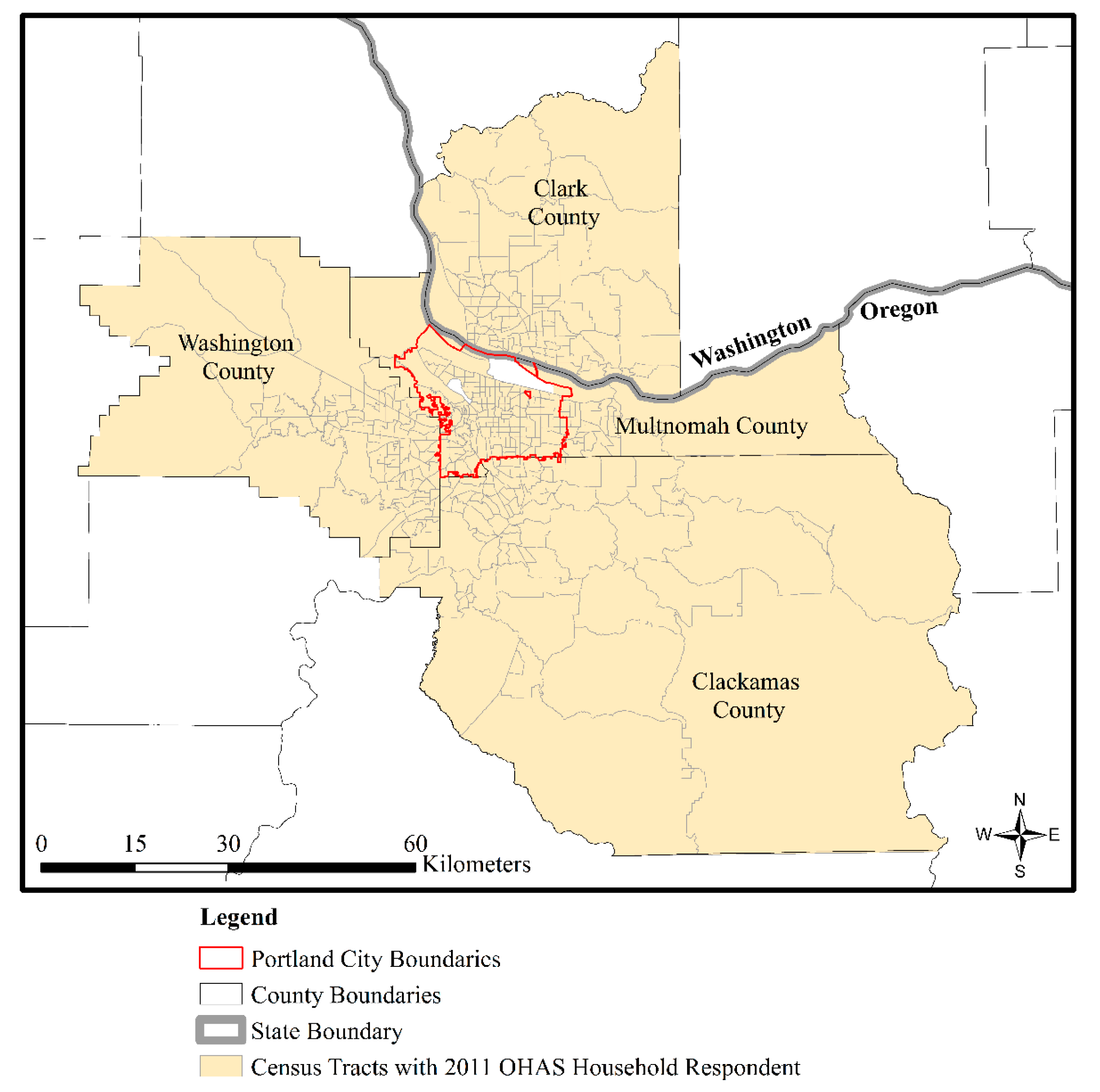
3.1. Sources, Samples, and Unit of Analysis

The Oregon Department of Transportation (ODOT) commissioned the OHAS and contracted with external survey professionals to develop and implement it. The contractors deployed a stratified random sample protocol throughout the ten Oregon regions at various points from 2008 to 2011, using a combination of addressed-based and landline and cell phone random digit dial frames [23,63]. In so doing, they aimed to derive representative proportional samples throughout the regions, and they oversampled “hard-to-reach demographic groups including low-income, Hispanics, African-Americans, large households and young households” [63] (p. 5). Sampling stratum were defined by household size and employment status with post-survey sample weights calculated based on socioeconomic and geographic factors throughout the regions [63].

The full OHAS dataset estimates daily household travel behavior for 17,941 households (and their members) during the study period [23]. Participating households kept a one-day travel diary and completed travel logs were collected via mail or telephone [23]. Our analytical sample included 6107 OHAS household respondents in the four-county Portland metropolitan area who completed their one-day travel diaries on weekdays in April and May 2011. We used geographic information systems to locate the 6107 households in 2010 census tract boundaries—our proxy for “neighborhood” and the primary unit of analysis featured in this study. Figure 1 displays the 457 census tracts that contained an OHAS household respondent in the four-county Portland metropolitan study area.

Our sample included responses for 4513 households in the three-county ODOT Region 1/Metro planning area (i.e., Clackamas, Multnomah, and Washington Counties) and 1594 households in the Southwest Washington Regional Transportation Commission (RTC) MPO transportation planning area of Clark County, Washington (i.e., home to Portland’s commuter city of Vancouver, Washington). As shown in Figure 1, all tracts in the metropolitan area counties of Clackamas (N = 80), Washington (N = 104), and Clark (N = 104), and 98.83 percent of tracts (N = 169 of 171) in Multnomah County contained an OHAS household respondent. Despite some missing cases that do not appear to be related to coding errors from the data source—but rather to an omission of data from the source itself—our initial sample (i.e., 6107 households) closely matches the sample of 6108 households studied in previous research [20,21]. In addition, our initial sample approaches approximately 95 percent of the OHAS data that ODOT Region 1 and Metro use to forecast travel demand and plan transportation projects in the Portland region.

We derived a number of tract-level variables from the 2011 OHAS, the 2010 US Decennial Census, and the 2008–2012 ACS [64]. These data sources allowed us to examine the representativeness of the 2011 OHAS against temporally matched data on aggregate- and tract-level racial composition. From these data sources, we also tested our guiding hypothesis in a multivariable spatial regression analysis. We omitted one inconsequential census tract in the southeastern corner of Clackamas County to arrive at a final analytical sample of 456 tracts in the spatial regression analysis. This omitted tract had a relatively high 2011 OHAS household response rate (see Figure 2) and low percentage of Latinx/Nonwhite householders (see Figure 3), but it was omitted because of missing data for a statistical control (median household income).

3.2. 2011 OHAS Houseohold Response Rate and Dependent Variable

We estimated the percent of occupied household respondents to the 2011 OHAS using the following procedures. After locating the OHAS household respondents, we divided the number of household respondents in a tract by the total number of occupied households in the tract from the 2010 US Decennial Census and turned the resulting ratio into a percent variable. We used the 2011 OHAS household response rate in three ways throughout our analysis. First, we described the distribution of the 2011 OHAS household response rates across our study area. Second, we ran bivariate correlations at the tract-level between the logged percent of 2011 OHAS household respondents (that approximates a normal distribution) and our explanatory and control variables. Third, we used the normally distributed, logged transformation of the OHAS household response rate as the dependent variable in our tract-level spatial regression model.

3.3. Householder Racial Identity and Explanatory Variable

The 2011 OHAS included a question about the householder’s racial identity that solicited responses similar to those obtained by the 2010 Decennial Census question regarding the householder’s racial identity by “Hispanic” or “Latino” “ethnic” status. We differentiated “Hispanic/Latino” status into non-Latinx and Latinx gender-neutral racial categories [29]. To assess the degree of racial misrecognition, we developed six comparable measures of household racial identification between the 2011 OHAS and the 2010 Decennial Census given similarities across the two datasets. The first was the percent of Latinx householders. For brevity, we dropped the “non-Latinx” status from the other householder racial identifiers and called these remaining measures the percent of householders that identify as White, Black, Indigenous (i.e., American Indian/Alaska Native), Asian, or Pacific Islander (PI)/Other/Multiracial. We used the weighted and unweighted count of 2011 OHAS household respondents in a tract, respectively, as the denominator for the weighted and unweighted OHAS householder racial identification variable. We used the number of total occupied households in a tract from the 2010 Decennial Census as the denominator for the census householder racial identification variables. To test our guiding hypothesis and arrive at a parsimonious spatial regression model, we aggregated the five POC census household racial identification variables into a single explanatory variable: percent of Latinx/Nonwhite householders.

3.4. Control Variables

In our spatial regression analysis, we controlled for other factors that were generally associated with household survey response rates [31,65]. We also controlled for factors suggested in the limited available OHAS technical documentation that are claimed to affect OHAS response rates [23,63].

Average median household income in the past 12 months (in 2012 inflation-adjusted USD) from the 2008–2012 ACS was our first control. We anticipated this variable would be positively associated with the OHAS household response rate due to the higher survey response rates typically found among higher income households, people, and places [31,32,33,34,35,36,37,38,39,40,41,42,43,44,45,46,47,48,49,50,51,52,53,54,55,56,57,58,59,60,61,62,63,64,65]. Five-year average estimates in the ACS can have margins of error as much as twice the estimate at finer geographic scales (e.g., census tracts and smaller) and for marginalized populations (e.g., low-income households, POCs, and inner-city residents) when compared to the 2000 census [31]. Accordingly, we assessed the data quality of the median household income estimate by calculating its coefficient of variation (CV). The CV is a standardized measure of the degree of uncertainty in an ACS estimate. To calculate the CV, we first had to derive a standard error of the estimate by dividing the published margin of error of the ACS estimate with a 90 percent confidence interval by 1.645. We then derived the CV by dividing the standard error of the estimate by the estimate [66]. Coefficient of variation thresholds are under the discretion of the researcher [67]. We used the CV threshold of 0.50 to achieve a medium-reliability level [68,69] and to minimize measurement error from the ACS and small analytical samples that might result from using more stringent CV thresholds [31,67].

Using the 2011 OHAS data and the 2010 Decennial Census count of the number of total occupied households in a tract as the denominator, we operationalized two variables that we posited to have a positive correlation with OHAS household response rates. The first was the percent of occupied households that were mailed an advanced letter about the 2011 OHAS. The second was the percent occupied households that received an incentive to participate in the 2011 OHAS. We used the first variable because sending letters to potential survey participants in advance of their receipt of the survey is an established procedure used by survey methodologists to prime and recruit participants to respond to the survey [65]. The OHAS administrators followed this practice in the context of its stratified random sampling protocol [23,63]. We incorporated the second variable into the analysis because offering incentives and compensation for survey participants can help to increase survey response rates [65]. Available technical documentation and the summary report for the 2011 OHAS in the Portland metropolitan area do not acknowledge the practice of offering incentives to increase response rates [23]. However, the household participant incentive indicator is in the data we obtained, and it was acknowledged in the technical document and final report for the OHAS in the ODOT Region 2, which borders our study area. As stated in that document: “Incentives were offered to targeted, hard-to-reach demographic groups (low-income, young, minority, and large households) in order to minimize unit non-response and provide a representative dataset” [63] (p. 1).

We developed two additional control variables from the 2010 Decennial Census. The first was the percent of individuals living in all group quarters in 2010. We included this variable because the OHAS’s sampling protocol did not target “residents living in group quarters (such as military personnel living on a base, students living in dormitories, and those in assisted living homes)” [23] (p. 2). Further, the spatial concentration of individuals living in such group quarters is typically associated with poorer survey estimates, as found in spatial analyses of census tract-level ACS data [31]. Thus, we expected this variable to be negatively associated with OHAS household response rates. Second, we accounted for the area of a census tract with a measure of tract square kilometers. The association between this variable and ACS estimate quality varies in both direction and magnitude across the United States [31]. Further, OHAS technical documentation states that “small geographic areas” had lower household response rates, but the exact meaning of “small” is unspecified in those statements [23]. We, therefore, included this final control in an effort to account for any possible association between tract size and OHAS household response rates.

3.5. Analytic Strategy

3.5.1. Assessing Racial Misrecognition in the 2011 OHAS: Aggregate and Tract Levels

The OHAS reflected the industry standard of using socioeconomic population characteristics in the initial stratification of the sampling frames and in the various post-survey weighting procedures. In so doing, OHAS administrators reportedly sought to align the samples with the 2000 Decennial Census and the 2007 (1 year) and 2006–2008 (3 year average) population estimates in the ACS [63]. The OHAS data analysts initially calculated a “household weight” to make the sample more representative of the target populations [63]. This is a standard “base weight” that is “the inverse probability of selection for each sample members”, which is used by survey methodologists to account “for any differences in sampled members’ chances of being selected into the sample” [65] (p. 87). The OHAS also included a “final household weight” or “household expansion factor” in our dataset [63]. Despite our efforts, we could not gain access to technical documentation that detailed how the household expansion factor was calculated for the 2011 OHAS in our Portland metropolitan study area. Given the preference for common OHAS protocols throughout the ODOT regions, however, we assumed it may have been calculated similarly to that for ODOT Region 2. In ODOT Region 2, the household expansion factor is a product of the household weight and adjustments for multiple cell phone numbers and a household ranking adjustment that, when summed, would equal the known population totals for household size, household income, workers in a household, and county of residence [63]. The household ranking adjustments included imputation for missing values, which was “based on an iterative proportional fitting procedure” and “involve[d] simultaneous ratio adjustments to two or more marginal distributions of the population counts” [63] (p. 14). Within ODOT Region 2, the household ranking adjustment was apparently successful in aligning the sample estimates to that of the target socioeconomic and geographic characteristics of the population.

To assess racial misrecognition in the 2011 OHAS, we compared aggregate- and tract-level householder racial identification across the 2010 Decennial Census and the unweighted and weighted 2011 OHAS samples. We calculated the weighted sample estimates by applying the household expansion factors to each householder’s racial identification and summing the weighted estimates of householders by their racial identification, in aggregate and at the tract level, for all householders in the 457 tracts that we included in this portion of the analysis. We compared those weighted estimates to the unweighted estimates from the 2011 OHAS and the 100 percent counts from the 2010 Decennial Census. In so doing, we anticipated that the OHAS estimates would not match the 2010 census counts because of (1) our guiding theoretical framework and case context discussed above; (2) the OHAS used earlier census and ACS data to calibrate the sample estimates; and (3) the OHAS primarily considered socioeconomic and geographic factors in constructing the weights.

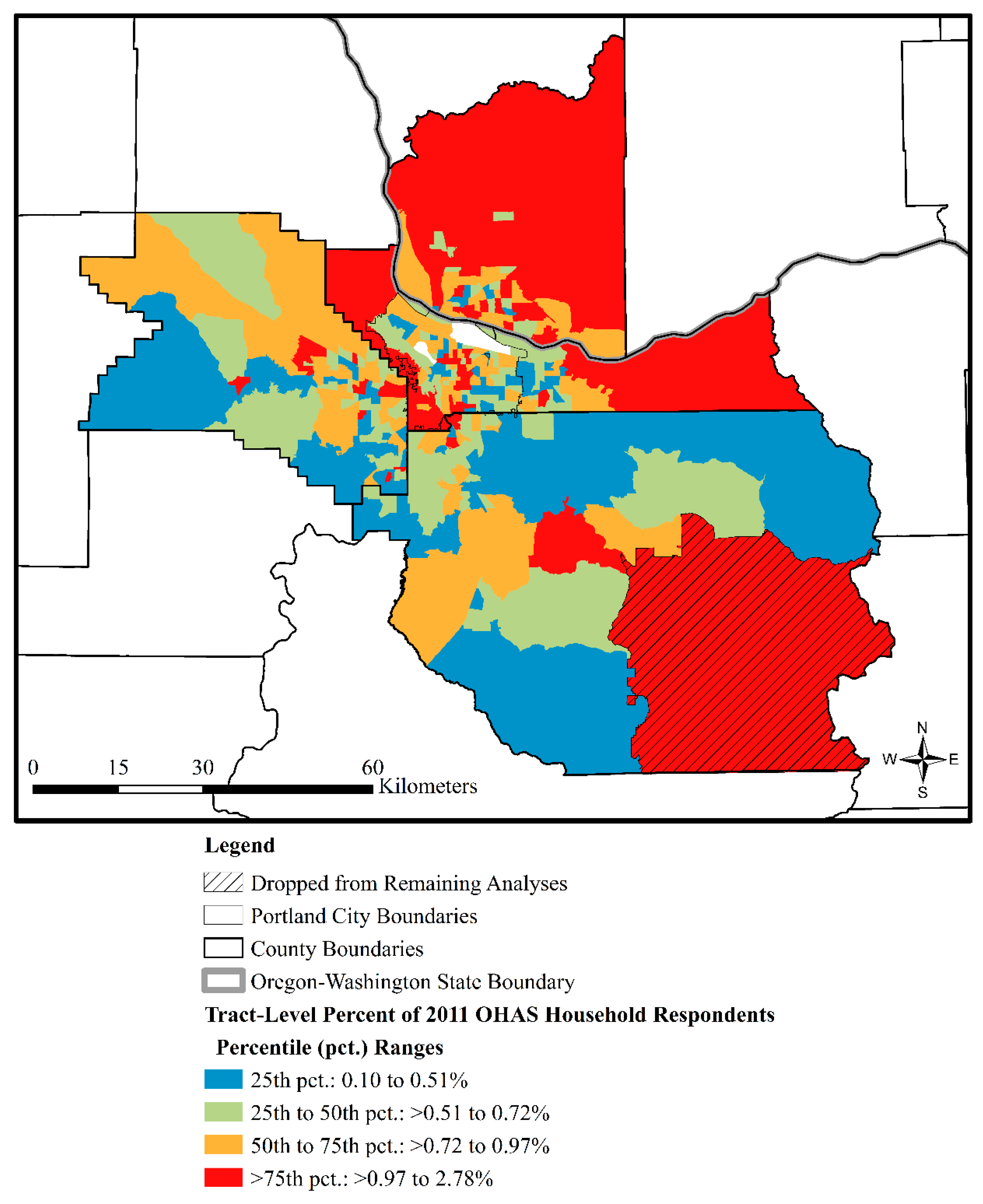
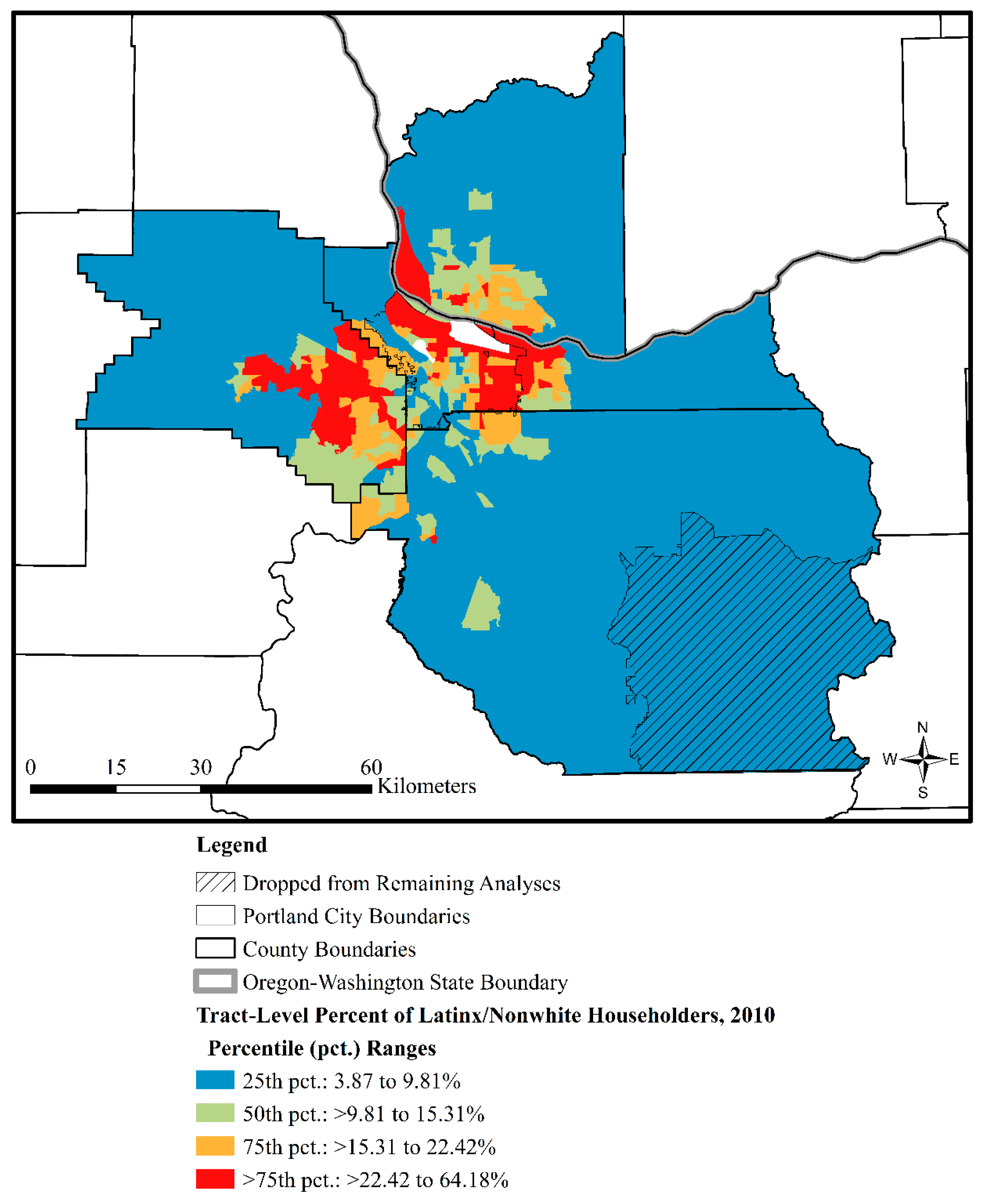
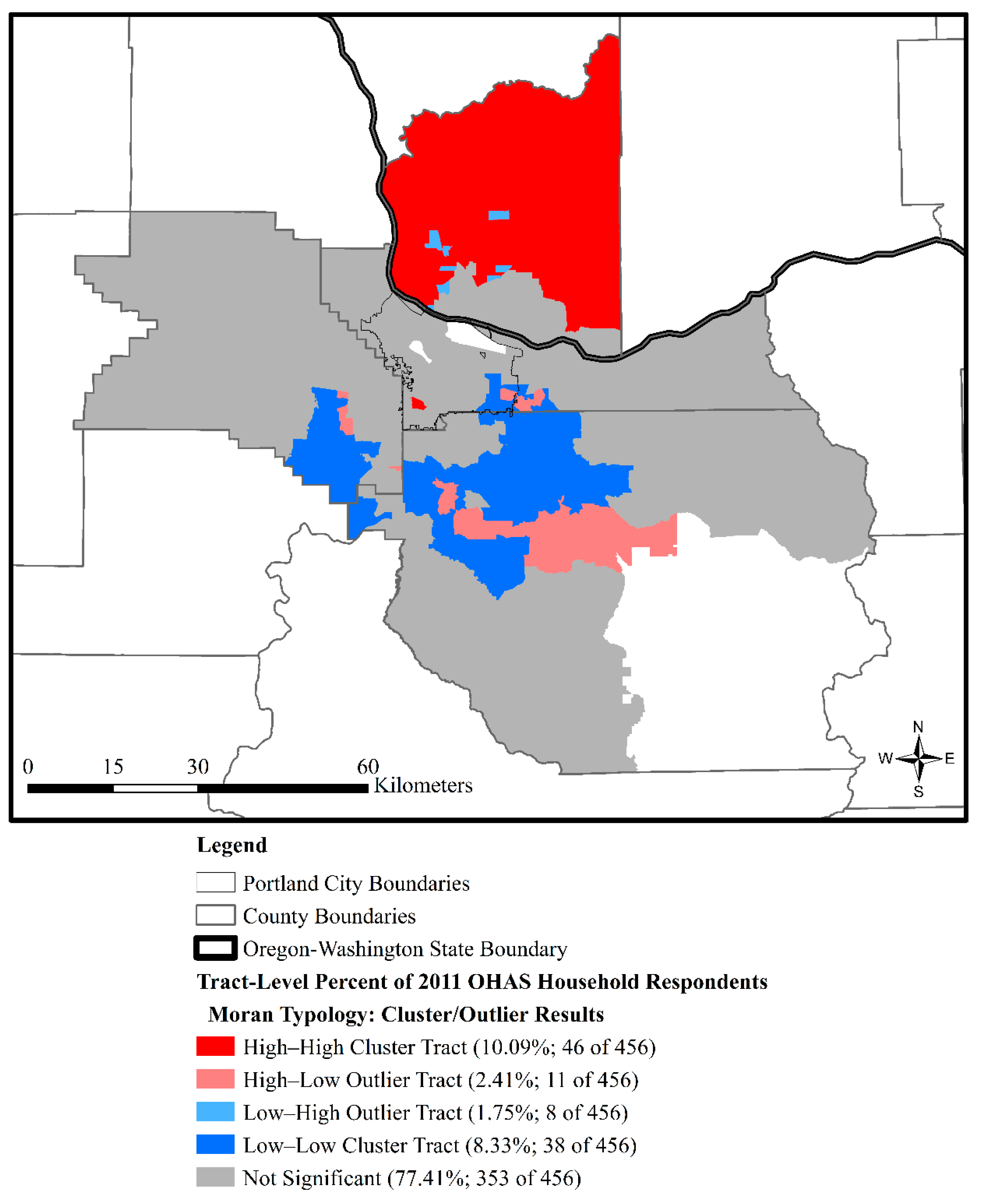
3.5.2. Tract-Level Univariate and Spatial Pattern Analyses

Following our assessment of the extent of racial misrecognition in the 2011 OHAS at the aggregate and tract levels, we transitioned to a tract-level analysis of variation in the OHAS household response rates, prevalence of Latinx/Nonwhite householders, and the control variables over the study area. In the process, we conducted a spatial pattern analysis of our primary variables of interest: the OHAS household response rate and householder racial identity.

Our spatial pattern analysis featured “global” and “local” indicators of spatial autocorrelation [70]. Spatial autocorrelation refers to ‘‘the correlation within variables across georeferenced space’’ [71] (p. 298). It is typically expressed with the “global” indicator of the Moran’s I, which tests the null hypothesis that the spatial distribution of attribute values at the tract level, for example, is due to random chance. Moran’s I values greater than 0 indicate spatial clustering, while values less than 0 indicate spatial dispersion and a value of 0 reflects a random spatial pattern.

The local indicator, Moran’s I_i, has a mean that is equal to the global Moran’s I. The Moran’s I_i measures the extent to which values across georeferenced space are most similar and dissimilar [70]. We defined the Moran’s I_i in the present study for tract i as:

$$I_i=Z_i{{\displaystyle \sum }}^{\text{}}{w}_{ij}{Z}_j$$

(1)

where $w_{ij}$ is the spatial weights matrix that operationalizes the spatial relationships between focal tract i and neighboring tract j; $Z_i$ and $Z_j$ are, respectively, standard deviations from the mean attribute values among tracts; and neighboring values are exclusively included in the summation over j [70]. We used a third-order queen adjacency spatial weights matrix in this portion of the analysis (and elsewhere in this study) to maintain consistency with multivariable spatial regression that drew on the same conceptualization of spatial relationships. We discuss this spatial weights matrix further in Section 3.5.3 and its strengths and limitations in our discussion of our results (Section 5).

The local Moran’s I_i produces a “Moran scatterplot” [70]. These results “characterize the typology of significant spatial associations around a focal unit of analysis based on whether the unit is above or below the mean for a given variable and its spatial lag” [72] (p. 54). In our analysis, we developed Moran typologies of tract-level OHAS household response rates and householder racial identification. In so doing, we identified tracts with high values that significantly clustered around similarly high values (“high–high” clusters) and tracts with low values that significantly clustered around similarly low values (“low–low” clusters). The Moran typology also classifies two forms of outlier tracts: “high–low” and “low–high” outliers. The former are tracts that have high values that are proximate to significantly low values, while the latter are tracts that have low values but are proximate to significantly high values. Tracts exhibiting no statistically significant distribution in their values receive a “not significant” classification within the typology.

We used an established Bonferroni correction procedure in our assessment of the statistical significance of the Moran’s I_i results [72,73,74,75,76]. This procedure addresses concerns over abnormality, multiple comparisons, and spatial autocorrelation in the distribution of the standard normal variates ($Z_i$). In the process, it controls the false discovery rate (FDR) of spatial clusters and outliers, which is the comparison-wise type I error rate of incorrectly rejecting the null hypothesis of the random spatial distribution. To implement the Bonferroni correction, we first calculated the number of “seemingly independent tests” of spatial patterning using the following equation:

$$v=n-r\left(n-1\right)$$

(2)

where v was the number of seemingly independent tests, r was the Moran’s I for the OHAS household response rate or the prevalence of Latinx/Nonwhite householders across census tracts, and n was the number of tests [72,73,74,75,76]. We then divided the standard p-value of 0.05 by the number of seemingly independent tests to determine the FDR-corrected p-value for classifying the significance of the cluster/outlier results for the OHAS household response rate and the prevalence of Latinx/Nonwhite householders.

3.5.3. Tract-Level Bivariate Correlation Analysis and Multivariable Spatial Regression Model

We conducted a bivariate correlation analysis to obtain preliminary understanding of the relationships between our dependent and independent variables prior to conducting our multivariable spatial regression analysis. In our multivariable regression analysis, we tested our study’s guiding hypothesis, which posited a negative association between the spatial concentration of Latinx and Nonwhite householders and the OHAS household response rates, net of other factors. We applied spatial econometric techniques to account for spatial effects in our regression analysis of the relationship between tract levels of logged OHAS household response rates and our explanatory and control variables. The Lagrange multiplier diagnostic tests of an initial ordinary least squares (OLS) regression model indicated the spatial error variant of the OLS model, estimated using a maximum likelihood technique, was the appropriate choice to account for those spatial effects in our regression analysis [77,78]. In using the spatial error model, we assumed that within-tract values of the logged percent of OHAS household respondents and our explanatory and control variables alone did not address spatial autocorrelation in the regression model and its error terms.

The spatial error model incorporates a spatially weighted error term (λWe) into the OLS regression equation. We defined our spatial error models as:

$$y= \alpha +{\displaystyle \sum }_k{\beta }_k{X}_k+\mathsf{\lambda }We+u$$

(3)

where $y$ represented the logged percent of OHAS household respondents, $\alpha$ was the constant, $\beta$ was the coefficient for the k number of X explanatory and control variables, λ was the spatial autoregressive coefficient, W was the spatial weights matrix, e was the OLS model random error term, and u was the spatially independent error term [68,77,78]. After considerable experimentation, we found that a third-order queen adjacency spatial weights matrix successfully accounted for spatial dependence in the spatial error model. This matrix resulted in a maximum of 101 and mean of 43 neighbors for the 456 tracts included in the spatial regression analysis.

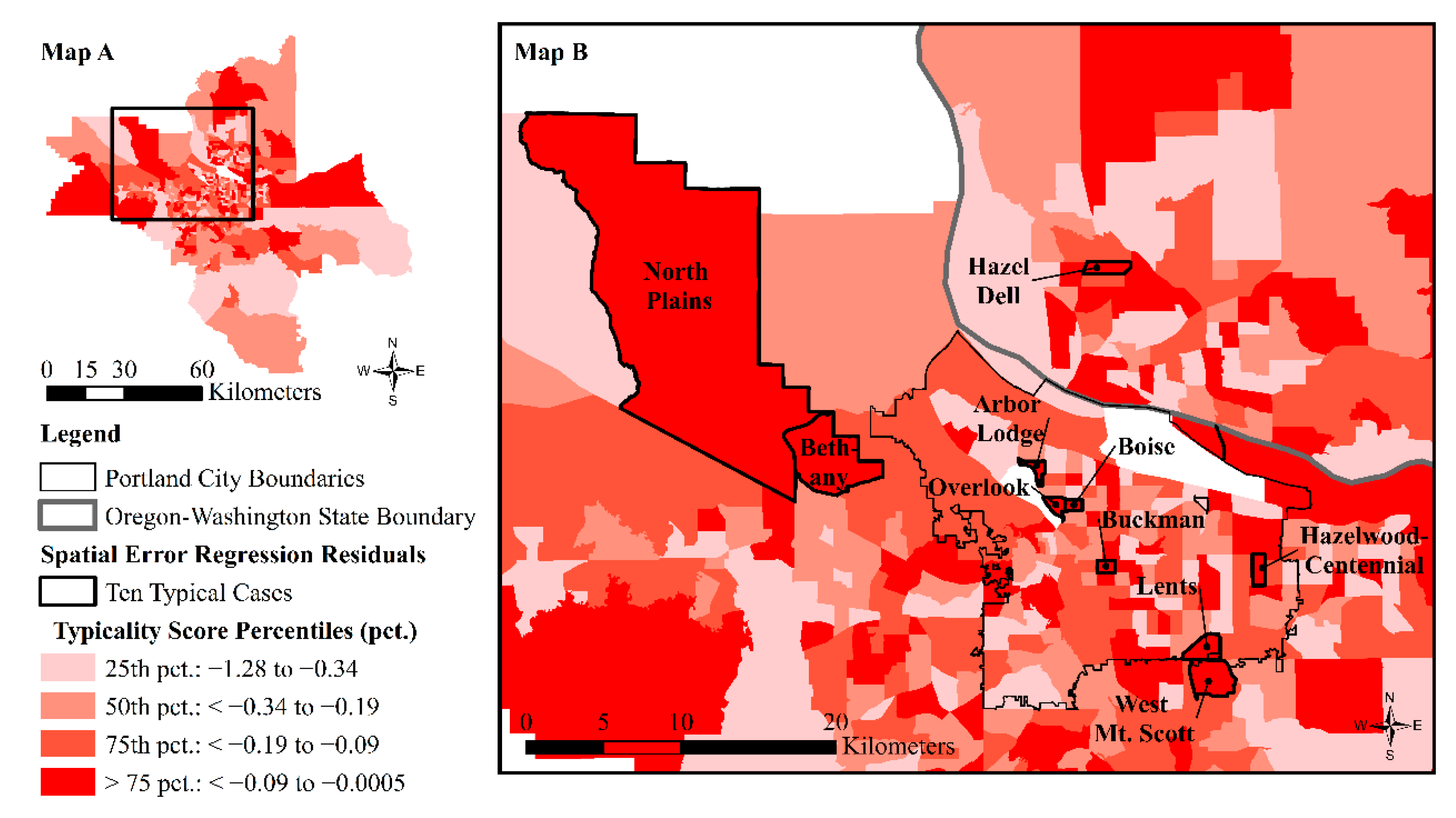
3.5.4. Identifying Ten Typical Cases

We systematically analyzed the residuals from the spatial error regression analysis to identify ten “typical” tracts out of the 456 in our final analytical sample that best represented the results from the regression analysis. In so doing, we sought to recognize the diverse racial characteristics of misrecognized neighborhoods in the OHAS. We also aimed to assess how patterns of racial misrecognition in these typical tracts corresponded with the results from our spatial pattern analysis and secondary source histories regarding dynamics of racial exclusion and socially unsustainable development in our study area. Furthermore, we used this portion of the analysis to identify areas for future research into the racial, spatial, and equity dimensions of sustainable transport and development in the Portland metropolis.

To be clear, the typical tracts we identified were not extreme or deviant examples of the results. Rather, their residuals from the regression analysis had the smallest absolute value and were by definition best representative of the association between tract-level householder racial identification and the OHAS household response rate, net of controls. We used the following formula adapted from Gerring [79] to identify the typical tracts:

$$\mathrm{Typicality}\left(i\right)= -abs[y_i-(a_i+{\displaystyle \sum }_{k_i}{\beta }_i{X}_i+\mathsf{\lambda }W{e}_i+u_i)]$$

(4)

where the “Typicality” of tract i equals $-$1 multiplied by the absolute value ($abs$) of tract i’s residual from the spatial error regression in Equation (3) as defined above. Typicality scores can theoretically vary from negative infinity to zero, with values closer to zero representing “onlier,” typical cases of the average pattern on the regression line that can direct future exploratory research on the relationships among the variables included in the analysis [79].

4. Results

4.1. Racial Representation and Misrecognition in the 2011 OHAS

Table 1. Aggregate and tract-level mean householder racial identification in the 2010 Decennial Census and the 2011 OHAS.

Householder Racial Identification	Data Source	Percent of Occupied Households
		Aggregate 1	Tract-Level Mean 2
Percent White	2010 Census	82.2	82.7
	2011 OHAS Unweighted	91.0	90.5
	2011 OHAS Weighted	90.2	90.0
Percent Latinx	2010 Census	6.9	6.8
	2011 OHAS Unweighted	2.5	2.8
	2011 OHAS Weighted	2.7	2.8
Percent Black	2010 Census	2.8	2.8
	2011 OHAS Unweighted	1.0	1.1
	2011 OHAS Weighted	1.2	1.2
Percent Indigenous	2010 Census	0.6	0.6
	2011 OHAS Unweighted	0.6	0.7
	2011 OHAS Weighted	0.8	0.9
Percent Asian	2010 Census	4.9	4.5
	2011 OHAS Unweighted	1.9	1.8
	2011 OHAS Weighted	2.0	1.9
Percent Pacific Islander, Other, or Multiracial	2010 Census	2.5	2.5
	2011 OHAS Unweighted	1.0	1.3
	2011 OHAS Weighted	1.1	1.2

¹ Aggregate percentages were out of 809,140 households for the 2010 Census; 6107 households for the 2011 OHAS unweighted sample; and 758,767 households for the 2011 OHAS weighted sample. ² Tract-level mean percentages were out of households in 457 census tracts. Percentages of householder racial identification for the 2011 OHAS unweighted and weighted samples do not equal 100 in the table because the table omits the percentage of householders who refused to provide racial identification in the OHAS.

compares householder racial identification in the 2010 Decennial Census against unweighted and weighted 2011 OHAS survey estimates in aggregate and at the tract levels. The majority of the 6107 OHAS householder respondents included in our sample identified as White (N = 5559, 91.03 percent). The remaining householder respondents identified as Latinx (i.e., “Hispanic”) (N = 152, 2.49 percent), Asian (N = 116, 1.90 percent), Black (or “African American”) (N = 60, 0.98 percent), or Indigenous (i.e., “American Indian or Alaska Native”) (N = 37, 0.61 percent). Another 63 (1.03 percent) of the householders identified as “Other”, which was primarily specified as “Multi-racial” or “Mixed”, different combinations of racial identities, the US census racial category of Pacific Islander, and a variety of other single identities not typically included in the US census general racial classification system. Notably, 120 (1.96 percent) householders refused to provide their racial identity.

As seen in Table 1, the 2011 OHAS consistently overrepresented White and underrepresented POC householders in the four-county Portland metropolitan study area. The aggregated 2011 OHAS unweighted and weighted percent of White householders exceeded the percent of White householders in the 2010 census by 8.8 and 8 percentage points, respectively. The 2011 OHAS achieved greater aggregate-level representation for Indigenous householders. However, it consistently underrepresented all other POC householders, especially Latinx and Asian householders, and to a lesser extent, Black householders. The tract-level patterns shown in Table 1 are generally consistent with the aggregate-level results in the table.

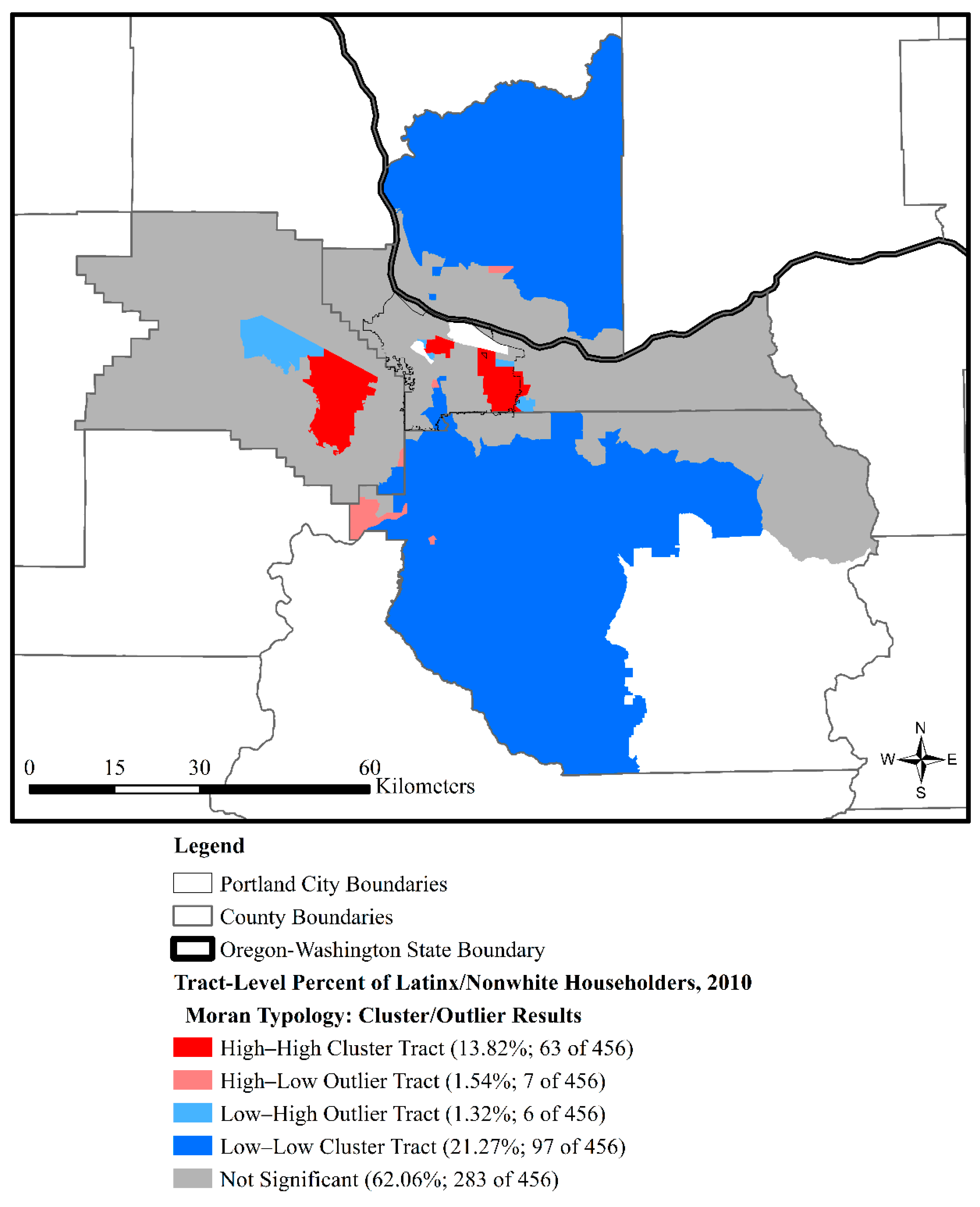
4.2. Tract-Level Descriptive Statistics and Spatial Pattern Analysis

Figure 2 displays the spatial distribution of the quartiles of the 2011 OHAS household response rate. It shows that around 75 percent of the 457 tracts included in this portion of the analysis had an OHAS household response rate below the statewide and Portland region response rate of 1 percent [22,23]. Figure 2 also shows that the upper quartile of the OHAS household response rate was spatially distributed through the urban core and periphery of the Portland metropolis. These spaces are receiving considerable investments in transportation infrastructure and becoming increasingly White and upper-class [25,58].

Figure 3 maps the distribution of quartiles of the percent of Latinx/Nonwhite householders from the 2010 Decennial Census in our study area. When read together, Figure 2 and Figure 3 elaborate on Table 1 by illustrating the spatial discrepancies between OHAS household response rates and Latinx/Nonwhite householder representation. In contrast to Figure 2, Figure 3 shows that the upper quartile of the percent of Latinx/Nonwhite householders was concentrated along the inner-ring suburban settlements around the urban core. These tracts are becoming increasingly Latinx, Nonwhite, economically disadvantaged, and excluded from transportation amenities [25,58].

Table 2. Descriptive statistics of variables used in the spatial error regression analyses (N = 456 tracts).

Variable	Mean	SD	Min.	Max.	Spatial Autocorrelation 1
					Moran’s I	Z-Score
OHAS household response rate
Percent of OHAS household respondents, 2011	0.783	0.381	0.104	2.521	0.229	23.610 ***
Natural log of percent OHAS household respondents, 2011	−0.362	0.497	−2.26	0.924	0.202	20.761 ***
Householder racial identity
Percent of Latinx/Nonwhite householders, 2010	17.308	9.383	3.873	64.183	0.347	35.618 ***
Control variables
Average median household income in past 12 months (thousands of 2012 inflation-adjusted USD), 2008–2012	61.544	21.172	13.699	148.832	0.111	11.581 ***
Percent of households that were mailed an advanced letter about the 2011 OHAS	0.088	0.083	0.000	0.476	0.065	7.003 ***
Percent of households that received an incentive to participate in the 2011 OHAS	0.296	0.196	0.000	1.332	0.200	20.708 ***
Percent of individuals living in all group quarters, 2010	1.557	4.68	0.000	47.419	0.027	3.300 **
Tract square kilometers	17.542	62.373	0.296	648.449	0.103	11.577 ***

¹ A third-order queen adjacency spatial weights matrix and 9999 permutations were used in the spatial autocorrelation analyses. *** pseudo p < 0.001; ** pseudo p < 0.01 (two-tailed test).

displays the descriptive statistics for the raw and logged versions of the OHAS household response rate, as well as for our explanatory variable, percent of Latinx/Nonwhite householders, and control variables that we used in the spatial error regression analysis. We presented these statistics for a slightly reduced analytical sample of 456 census tracts with non-missing data. Table 2 elaborates on Figure 2 and Figure 3 by showing that the raw and natural log transformation of the OHAS household response rates were relatively dispersed (Moran’s I = 0.229, z-score = 23.610; Moran’s I = 0.202, z-score = 20.761, respectively, pseudo p < 0.001) when compared to the percent of Latinx/Nonwhite householders (Moran’s I = 0.347, z-score = 35.618, pseudo p < 0.001).

Table 2 also introduces the relatively limited variation in the control variables with regard to their values and spatial distribution. Tract square kilometers, average median household income from 2008 to 2012, and the percent of individuals living in group quarters as of 2010 have the greatest variation in values, but those values exhibit low levels of spatial clustering (Moran’s I ≤ 0.111, z-scores ≤ 11.581, pseudo p < 0.001). In addition, the percent of households that received an incentive to participate in the 2011 OHAS exhibited more variation in values and more spatial clustering (Moran’s I = 0.200, z-score = 20.708, pseudo p < 0.001) than the percent of households that were mailed an advanced letter about the 2011 OHAS (Moran’s I = 0.065, z-score = 7.003, pseudo p < 0.001). The variation in the percent of incentivized households is likely attributed to the targeted efforts of the OHAS surveyors to incentivize participation by POC householders, whom are moderately spatially clustered in the metropolis [23,63].

Figure 4 and Figure 5, respectively, display the cluster and outlier results from the local Moran’s I_i analysis for the raw 2011 OHAS household response rate and the percent of Latinx/Nonwhite householders in 2010 throughout the Portland metropolitan study area. The Bonferroni-adjusted statistical significance thresholds ($p_{\mathrm{BONV}})$ differed slightly for the two variables given their different global levels of spatial autocorrelation. Inserting the global Moran’s I of 0.229 into Equation (2) results in 350.805 seemingly independent tests and a $p_{\mathrm{BONV}}$ = 0.05/350.805 = 0.00014 for the OHAS household response rate. Similarly, inputting the global Moran’s I of 0.347 into Equation (2) results in 298.115 seemingly independent tests and a $p_{\mathrm{BONV}}$ = 0.05/298.115 = 0.00017 for the percent of Latinx/Nonwhite householders. These Bonferroni-adjusted statistical significance thresholds are far more conservative than the traditional p < 0.05 threshold and increased our confidence in the Moran typology we present in Figure 4 and Figure 5.

It is instructive to compare Figure 4 to Figure 2. Figure 2 generally shows that higher OHAS household response rates were distributed around the Portland City core and in some peripheral suburban and rural spaces of the metropolis—many of which are privileged socially and in the metropolitan transportation system [25,58]. However, Figure 4 demonstrates that there were two statistically significant clusters of high OHAS household responses rates. One such cluster included two tracts in Southwest Portland. The other, much larger cluster of high OHAS household response rates, covered 42 percent (N = 44) of the tracts in Clark County, Washington, just outside the cities of Vancouver and Camas. In contrast, the clusters of low OHAS household response rates manifested throughout two distinct regions of the metropolis. The first resided in the southwest portion of the metropolis, forming a continuous cluster from one tract in rural western Clackamas County to six more tracts in Southeast Washington County near Sherwood City. The other cluster of low OHAS household response rates included 31 contiguous tracts: 12 at the East Portland–Southwest Gresham interface which are adjacent to 19 other contiguous Clackamas County tracts from Happy Valley westward to Stafford and southward to Mulino.

Comparing Figure 3 and Figure 5 illuminates the spatial patterns in the percent of Latinx/Nonwhite householders. Figure 3 generally shows that in 2010, Latinx/Nonwhite householders concentrated along the inner-ring, lower status suburban settlements with limited transportation amenities [25,58]. In Figure 5, we see three relatively compact clusters of high concentrations of Latinx/Nonwhite householders in the metropolis. One such cluster included 27 tracts in East Washington County at the meeting of Aloha and the cities of Hillsboro and Beaverton. Another cluster of high concentrations of Latinx/Nonwhite householders included 10 tracts in Northeast Portland. The other high–high cluster of Latinx/Nonwhite householders included 26 contiguous tracts, occurring once again at the East Portland–Southwest Gresham border. The clustering of low concentrations of Latinx/Nonwhite householders exhibited a starkly different spatial pattern. Figure 5 shows an island tract in Vancouver, Washington; 33 contiguous tracts outside of Vancouver in northern Clark County (where the high OHAS household response rates cluster); and a contiguous cluster of 63 tracts stemming from the Portland neighborhood of Buckman through Southcentral Portland to 55 tracts covering much of Clackamas County.

4.3. Bivariate Correlations

Table 3. Pearson correlation coefficients for variables used in the spatial error regression analyses. (N = 456 census tracts).

Variables	1	2	3	4	5	6
1. Natural log of percent OHAS household respondents, 2011
2. Percent of Latinx/Nonwhite householders, 2010	−0.388 ***
3. Average median household income in past 12 months (thousands of 2012 inflation-adjusted USD), 2008–2012	0.332 ***	−0.417 ***
4. Percent of households that were mailed an advanced letter about the 2011 OHAS, 2010–2011	0.377 ***	−0.024	−0.028
5. Percent of households that received an incentive to participate in the 2011 OHAS, 2010–2011	0.420 ***	0.012	0.172 ***	0.488 ***
6. Percent of individuals living in all group quarters, 2010	−0.095 *	0.045	−0.197 ***	0.051	0.051
7. Tract square kilometers	−0.013	−0.265 ***	0.080	−0.029	−0.031	−0.046

* p < 0.05; *** p < 0.001 (two-tailed test).

presents the bivariate correlations among the variables used in the spatial error regression analysis. The table shows a null association between the percent of Latinx/Nonwhite householders and the percent of households that received an incentive to participate in the OHAS—despite the OHAS surveyors’ efforts to target their incentives to POC householders. Table 3 also illustrates that our independent variables are not highly correlated, and an initial indication that the model we present in Section 4.4 is parsimonious. Further, the majority of the bivariate correlations between our independent variables and the natural log of the percent of OHAS household respondents were all significant and signed as expected. The lone exception to this pattern was the null association between the logged OHAS household response rate and tract square kilometers. The direction of the association among these variables was not clear from previous research [31] and the OHAS technical documentation [23], but it was at least thought to be a significant association. Table 3 indicates that that expectation may not be warranted.

To understand the bivariate relationship between survey participation incentives and householder racial identity further, we compared the extent to which different racial groups of householders were more likely to receive an incentive to participate in the 2011 OHAS. We found that Indigenous householders were 3.63 times more likely to receive an incentive (N = 29) than not (N = 8), which may have helped the OHAS derive a more representative sample of Indigenous householders in the Portland metropolis. Interestingly, the majority of the Latinx (N = 107 of 152; 70.39 percent), Black (N = 42 of 60; 70.00 percent), and Asian (N = 75 of 116; 64.66 percent) householder participants were respectively 2.38, 2.33, and 1.83 times more likely to receive an incentive than not. However, these racial groups of householders were consistently underrepresented in the OHAS. Pacific Islanders, other Nonwhite or Multiracial householders were also underrepresented in the OHAS, but the majority of them (N = 34 of 63; 53.97 percent) were 0.85 times less likely to receive an incentive. On the other end of the spectrum, White householders were 60 times less likely to receive an incentive (N = 2093) than not (N = 3466), and White householders were overrepresented in the OHAS. Thus, OHAS surveyors targeted many POC householders with incentives to participate, but racial misrecognition still pervades the OHAS.

4.4. Multivariable Spatial Error Regression Analysis

Table 4. Spatial error regression results for natural log of percent of 2011 OHAS household respondents in the four-county Portland metropolitan study area (N = 456 census tracts).

Variables	b	S.E.	B
Householder racial identity
Percent Latinx/Nonwhite householder, 2010	−0.017 ***	0.002	−0.323
Control variables
Average median household income in past 12 months (thousands of 2012 inflation-adjusted USD), 2008–2012	0.003 ***	0.001	0.149
Percent of households that were mailed advanced letter about the 2011 OHAS, 2010–2011	0.559 **	0.207	0.093
Percent of households that received an incentive to participate in the 2011 OHAS, 2010–2011	1.244 ***	0.097	0.490
Percent of individuals living in all group quarters, 2010	−0.007 *	0.003	−0.070
Tract square kilometers	−0.001 **	0.000	−0.089
Constant	−0.697 ***	0.178
Lambda (λ)	0.910 ***	0.045
Multicollinearity condition index	12.736
Pseudo R2	0.613
Log likelihood	−120.471
Degrees of freedom	449
Akaike information criterion	254.942
Moran’s I of residuals 1	−0.009

¹ The spatial autocorrelation analysis of regression residuals used a third-order queen adjacency spatial weights matrix and 9999 permutations. * p < 0.05; ** p < 0.01; *** p < 0.001 (two-tailed test).

displays the results from our spatial error regression analysis. The results show that the percent of Latinx/Nonwhite householders had a highly significant negative association with the OHAS household response rate. This finding supports our guiding hypothesis, which posited that the spatial concentration of Latinx and Nonwhite households would be negatively associated with OHAS household response rates, net of controls. As shown in Table 4, a one-point increase in the percent of Latinx/Nonwhite householders in 2010 was associated with a statistically significant 1.7 percent decrease in the logged percent of OHAS household respondents in our sample of 456 tracts.

The results for all of the control variables were significant and as expected given previous research within and beyond the OHAS and Portland metropolitan area case [23,31,63,65]. Net of other factors in the model, average median household income levels, and the percentages of households that were mailed an advanced letter about OHAS and that received an incentive to participate in the OHAS were positively associated with the OHAS household response rate. Similarly, as expected from previous research [23,31], the percent of individuals living in all group quarters was negatively associated with the OHAS household response rate. Further, in the context of the other factors included in the spatial error regression model, tract square kilometers had a significant, negative association with the OHAS household response rate.

The highly statistically significant Lambda and the insignificant Moran’s I for the spatial error regression residuals indicate the spatial error model successfully addressed spatial dependence in the analysis. The spatial error regression model’s multicollinearity condition index of 12.736 is well below the suggested threshold of 30 [70], which further indicates the model is parsimonious and not impeded with concerns about collinearity between the explanatory and control variables. In addition, the factors included in the model account for approximately 61.3 percent of the variance in the OHAS household response rate. The standardized coefficients (B) for the variables in the model aid in identifying the relative magnitude of the associations between the independent variables and the logged OHAS household response rate, as values farther from zero indicate stronger associations. The standardized coefficients indicate that, among those factors considered in the model, the top three determinants of the census tract-level 2011 OHAS household response rate were the percent of households that received an incentive to participate in the 2011 OHAS, followed by the percent of Latinx/Nonwhite householders and average median household income in the past 12 months.

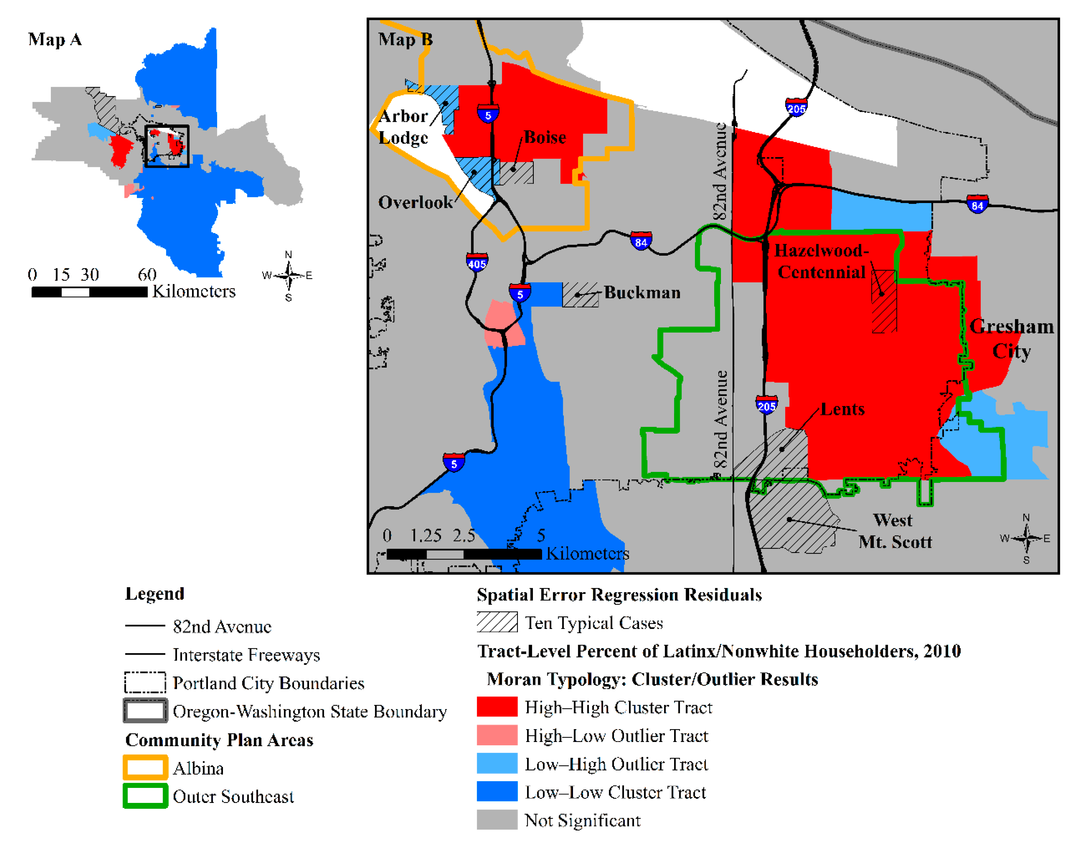
4.5. Typical Representations of Low OHAS Household Response-High Latinx/Nonwhite Householder Tracts

Figure 6 maps the spatial distribution of typicality scores for the residuals from the spatial error regression analysis. The ten typical tracts have typicality scores ranging from −0.01 to −0.0005, and they best represent the negative association between tract-level Latinx/Nonwhite householder identification and the OHAS household response rates, net of other factors in the analysis. As shown in Appendix A,

Table A1. Comparison of household racial identification in the 2010 Decennial Census and the 2011 OHAS in ten typical cases from the spatial error regression results in the Portland metropolitan study area.

Racial Composition 1	Data Source	Tract Name
		Arbor Lodge	Bethany	Boise	Buckman	Hazel Dell	Hazelwood– Centennial	Lents	North Plains	Overlook	West Mt. Scott
Percent White	2010 Census	85.20	74.30	59.50	88.80	75.30	71.40	76.60	92.50	83.00	78.60
	2011 OHAS Unweighted	70.00	77.80	83.30	82.40	76.90	75.00	100.00	93.30	83.30	85.70
	2011 OHAS Weighted	84.40	78.40	89.50	81.90	83.60	67.90	100.00	95.70	88.70	89.30
Percent Latinx	2010 Census	4.30	6.50	5.20	4.20	12.10	10.10	8.90	4.40	3.70	3.70
	2011 OHAS Unweighted	10.00	0.00	0.00	0.00	0.00	0.00	0.00	0.00	0.00	0.00
	2011 OHAS Weighted	3.70	0.00	0.00	0.00	0.00	0.00	0.00	0.00	0.00	0.00
Percent Black	2010 Census	3.90	2.30	28.50	1.30	3.50	6.80	3.30	0.10	5.60	1.50
	2011 OHAS Unweighted	0.00	11.10	16.70	0.00	0.00	12.50	0.00	0.00	16.70	0.00
	2011 OHAS Weighted	0.00	10.80	10.50	0.00	0.00	6.60	0.00	0.00	11.30	0.00
Percent Indigenous	2010 Census	0.60	0.50	0.70	0.70	0.60	1.10	0.60	0.30	0.90	0.30
	2011 OHAS Unweighted	0.00	0.00	0.00	0.00	0.00	0.00	0.00	0.00	0.00	0.00
	2011 OHAS Weighted	0.00	0.00	0.00	0.00	0.00	0.00	0.00	0.00	0.00	0.00
Percent Asian	2010 Census	2.40	13.10	1.60	1.90	5.40	8.40	7.80	1.40	2.90	14.00
	2011 OHAS Unweighted	0.00	11.10	0.00	5.90	7.70	0.00	0.00	6.70	0.00	7.10
	2011 OHAS Weighted	0.00	10.80	0.00	12.70	7.40	0.00	0.00	4.30	0.00	5.40
Percent Pacific Islander, Other, or Multiracial	2010 Census	3.60	3.30	4.50	3.10	3.20	2.30	2.80	1.20	3.70	1.90
	2011 OHAS Unweighted	10.00	0.00	0.00	11.80	7.70	12.50	0.00	0.00	0.00	7.10
	2011 OHAS Weighted	6.80	0.00	0.00	5.50	5.10	25.50	0.00	0.00	0.00	5.40
N households	2010 Census	1270.00	1252.00	1358.00	2669.00	2052.00	1580.00	1495.00	1789.00	855.00	2361.00
	2011 OHAS Unweighted	10.00	9.00	6.00	17.00	13.00	8.00	6.00	15.00	6.00	14.00
	2011 OHAS Weighted	1026.60	903.20	917.20	1833.30	1474.20	966.40	315.90	1326.10	739.70	2385.70
Percent of 2011 OHAS Household Respondents		0.79	0.72	0.44	0.64	0.63	0.51	0.40	0.84	0.70	0.59

¹ Percentages of householder racial identification for the 2011 OHAS unweighted counts and weighted estimates do not equal 100 in the table because the table omits the unweighted counts and weighted estimates of the percent of householders who refused to state their racial identity on the OHAS.

, the percent of OHAS household respondents varied from 0.40 percent in the Lents tract to 0.84 percent in the North Plains tract. In addition, the OHAS household response rate averaged 0.63 percent across these ten representative tracts—thus, below the statewide and Portland region response rate of 1 percent [22,23]. These ten typical tracts are placed in the broader context of the 456 tracts that were analyzed in the regression analysis in Figure 6, Map A, and labeled in the detailed Map B in Figure 6. Continuing the patterns discussed above, Figure 6B illustrates how these representative tracts reside along the peripheral urban and suburban spaces of the metropolis that are increasingly home to transportation disadvantaged POC and low-income households, while inner-city Portland has become more White, affluent, and flush with transportation amenities [25,58].

Further analysis indicates that racial misrecognition of the OHAS data is evident to various extents in these ten typical tracts. The most glaring manifestation of racial misrecognition occurred for Indigenous and Latinx householders. As shown in Appendix A, Table A1, the OHAS recorded no Indigenous householders in these typical tracts despite the 2010 Decennial Census enumerating low shares of Indigenous householders in them. Latinx householders were more prevalent in these tracts, according to the 2010 Decennial Census. However, the 2011 OHAS only accounted for their presence in the Arbor Lodge tract. The 2011 OHAS better represented Asian, Pacific Islander, other Nonwhite, Multiracial, and Black householders, albeit unevenly, across nine of the ten typical tracts. The lone exception to this pattern was in the Lents tract, which had 23.4 percent Latinx/Nonwhite householders according to the 2010 Decennial Census but 100 percent White householders in the 2011 OHAS. Overall, Table A1 shows that the 2011 OHAS better represented—and often overrepresented—White householders in the ten typical tracts. In addition to the Lents case, White householders were markedly overrepresented in the Boise and West Mt. Scott tracts to the point that their respectively high shares of Black, Asian, and other Nonwhite householders were underrepresented or completely unrecognized in the 2011 OHAS.

These exemplar tracts of racial misrecognition are reproductions of other historical and contemporary racial and spatial inequalities in the metropolis. As shown in Figure 7, three of these tracts—Arbor Lodge, Overlook, and Boise—border the Northeast Portland cluster of Latinx/Nonwhite householders that we detected in our analysis. Together, these spaces constitute much of what has more recently been known to the City of Portland as “the Albina Community Plan Area” and the controversial “Interstate Corridor” urban renewal area along Interstate 5 that has been unsuccessful in halting gentrification and displacement [58,80]. However, scholars and community members commonly refer to that area, including the racially misrecognized Boise tract as described above, as “Upper Albina” [56]. Historically, “Lower Albina” typically refers to neighborhoods south of Boise, between Northeast Fremont Street and Interstate 84 [56].

Upper Albina became the center of Portland’s Black community in the 1960s and 1970s following a number of racially unjust and socially unsustainable developments [81]. First, political disenfranchisement and systemic labor and housing market discrimination in Portland and Oregon prior to 1940 concentrated small numbers of marginalized Blacks, other POCs, and low-income immigrants in north downtown (near the contemporary site of Union Station) and in the nearby Lower Albina neighborhood of Eliot, just south of Boise [24,56,81]. Second, in the 1940s, thousands of Black migrants to the metropolis were restricted to World War II-era defense housing in Vanport City, north of Portland, in the Guild’s Lake area of Northwest Portland, or within the narrow confines of the Eliot and Boise neighborhoods [81]. Then, in 1948, a disastrous flood, permitted by government officials’ discriminatory flood protection, destroyed Vanport and displaced its Black residents to where other Blacks were already restricted: Lower and Upper Albina [24,56,81]. More labor and housing discrimination against Black Portlanders continued, and was coupled with urban renewal, Interstate 5 development, and “blight clearance” of disinvested Black, other POC, and low-income immigrant neighborhoods from the 1950s to 1970s, which pushed those marginalized groups farther into Upper Albina neighborhoods [24,25,56,58,81]. These neighborhoods include the contemporary cluster of high concentrations of Latinx/Nonwhite householders adjacent to Arbor Lodge, Overlook, and Boise shown in Figure 7.

More recently, Blacks and other POCs have been displaced from Upper Albina to suburban settlements in North, Northeast, and East Portland due to the number of gentrifying “urban sustainability fixes” [82]. These investment strategies respond to popular environmental concerns, municipal fiscal imperatives, and private real estate interests through the “green investments” in physical infrastructure and urban redevelopments that increase land values and “attract affluent, well-educated, environmentally minded residents and the businesses that cater to their interests” [58] (p. 8). Within Portland, sustainability fixes have primarily manifested through bike lanes, light rail, pedestrian-friendly neighborhoods, and infill construction [25,58]. Portland’s sustainability fixes also include the promotion of farmers’ markets and urban agriculture [28], and the arts and creative industries [59,61,83].

Figure 7 also shows the north–south corridor of 82nd avenue, which has emerged from Portland’s history of racial exclusion and socially unsustainable development as an important symbolic and material boundary that demarcates the devalued, racially diverse, and low-income East Portland suburbs from Portland’s gentrifying, increasingly White, and “sustainable” urban core [25,28,58,59]. Indeed, the bulk of Portland’s sustainability fixes since the 1990s have been concentrated west of 82nd Avenue, while much of the area east of 82nd avenue during that time span has been subjected to various commercial, housing, transportation, public safety, and planning “revitalization” efforts per Portland’s Outer Southeast Community Plan Area [58,80,84]. Despite these earlier efforts and the more recent 2009 East Portland Action Plan, much of East Portland has been neglected through two parallel developments. First, a regressive statewide property tax system instituted in the 1990s benefited Portland’s gentrifying urban core and penalized the devalued homes and properties owned in East Portland [58]. Second, the City of Portland has exercised lax enforcement of decentralized infrastructure payment mechanisms that results in “a haphazard mosaic of old and new construction, incomplete sidewalks, gravel cul-de-sacs, potholes, and unpaved streets” [58] (p. 14). Meanwhile, East Portland and its neighboring Gresham City are fraught with political contestation over gentrification and serial displacement of racially and economically marginalized renters [85].

Within this context of racial exclusion and socially unsustainable development in East Portland, we found three additional tracts: Hazelwood–Centennial, Lents, and West Mt. Scott. Hazelwood–Centennial resides at the center of the Latinx/Nonwhite householder cluster in East Portland. Lents and West Mt. Scott border that cluster. However, both Lents and West Mt. Scott reside within another cluster we found in our analysis: the large cluster of low 2011 OHAS household response rates that meander from East Portland–Southwest Gresham southward through Northwest Clackamas County (see Figure 4). Our analysis indicates that these three tracts are exemplars of low OHAS household response rates, high concentrations of Latinx/Nonwhite householders, and racial misrecognition. Among these three tracts and the other typical tracts we identified in our analysis, Lents stands out because the 2011 OHAS represents it as 100 percent White and, thus, misrecognizes its diversity and fails to include any of its Latinx, Black, Indigenous, Asian, or other POC householders (see Table A1).

5. Discussions

The US FTA [39] recognizes racial “minorities” as a protected class and it requires transit agencies to demonstrate that policies and fare changes do not disproportionately affect low-income populations. Yet, nationwide household travel surveys inadequately represent people of color and other protected classes. We know even less about the associated non-coverage and non-response errors of household transportation surveys at the regional and local levels, especially in Oregon and in the Portland metropolitan area. Consistently throughout our analysis, we found that the 2011 OHAS underrepresented racial minority households in aggregate and at the tract-level across the Portland metropolis. Accordingly, we have limited understanding of how different racial minorities, as a federal protected class, experience the transportation system in the Portland region. The implications of racial misrecognition in the OHAS must be better understood given how these data are used by the ODOT and MPOs—like the Portland’s Metro—to forecast travel demand and develop long-range transportation plans. These data gaps are particularly troubling given the challenges that vulnerable POCs often face in Portland; modeling from an unrepresentative sample risks obscuring the unique vulnerabilities of marginalized groups [20,73].

We acknowledge that the OHAS data processors sought to minimize non-coverage and non-response errors and ensure representative samples [63] in a way that “conformed to industry standards” [23]. Indeed, the stratification and post-stratification criteria applied to the OHAS conformed with the preference for using “functional” socioeconomic factors over “ambiguous demographic” factors of race in transportation planning and analysis [2,49]. As the results of this study suggest, these methodological choices—perhaps in interaction with systemic Latinx/Nonwhite non-response to the OHAS which could be due to a number of factors including distrust in official surveys [15,34,35,36,37]—contributed to consistent misrepresentation of Latinx/Nonwhite householders and overrepresentation of White householders throughout the four-county Portland, Oregon metropolitan area. We understand this problem of representativeness through the lens of justice and racial theories as a problem of “racial misrecognition” in which racial group difference is obscured and foundational for distributive transportation inequities and unsustainability that is manifest throughout the Portland metropolitan area [20,21,25,54,56,58].

Survey administrators and even some transportation planners may not have much ability or authority to intervene into the unsustainable and inequitable distribution of transportation amenities in the Portland area. However, transportation surveyors and planners should be aware of the consequences of their seemingly race-neutral actions [2], and the important sociological insight that racial categories, identities, processes, and outcomes within and beyond the Portland, Oregon transportation sector are not reducible to social class [1,2,10,11,28,29,48,50,51,52,53,55,56,58,59,60,61,62,68,69,72,81,83]. Indeed, racial misrecognition in the 2011 OHAS occurred even when the samples were weighted to make them more representative of socioeconomic factors in the metropolis. Elaborating on this point, some of the most prominent survey researchers in the world state the following implications of such methodological choices, particularly as they relate to weighting:

“Most surveys are weighted only to demographic characteristics because these are the most widely available measures available on sample files and in the data sets people weight to. This brings us to an important limit of weighting. Weighting on any characteristic will ensure that the sample is representative with respect to that characteristic and to characteristics that are correlated with it, but it will not ensure that the sample is representative with respect to characteristics that are not correlated with the characteristic used for weighting. This means that within the same survey, weighting can improve some estimates, have no effect on others, and potentially even bias others”.

[65] (p. 89)

Given these considerations about weighting and the findings from our study, we suggest an alternative pathway moving forward to address the systemic problem of racial misrecognition in the OHAS, reflected throughout the broader practice of household transportation surveys in the United States. First, one-day travel log surveys may be the preferred mode of efficiently obtaining snapshots of people’s travel behavior within the OHAS [22,23,63]. However, research illustrates how routine variation in travel behaviors are commonly missed with single-day activity surveys [86]. Further, the findings reported in this study suggest that, in the case of the OHAS, sole reliance on one-day travel logs contributes to highly problematic patterns of racial misrecognition in household travel surveys and the reproduction of racialized and spatialized transportation inequities and social unsustainability in the Portland area.

Bricka [23] indicates that recent advances in household travel surveys could help overcome some of the limitations of irregular, single-day activity survey and other techniques featured in the 2011 OHAS. Such advancements entail address-based sampling techniques that draw on increasingly holistic household contact, demographic, and consumer data that was not available from venders during the implementation of the 2011 OHAS. Other improvements to OHAS may rest in including cost-effective annual surveys of smaller household sampling sizes; inclusion of global positioning systems (GPS), smartphone, and internet-based data collection techniques “to reduce respondent burden and increase data quality, and the evaluation of passive data to complement and supplement traditional travel survey data” [23] (pp. 43–44).

Dillman et al. [65] may agree that such mixed-mode survey methodologies and techniques could offer important ways to align household travel surveys with the “tailored design method”. This method is premised on the argument that “in order to minimize total survey error, surveyors have to customize or tailor their survey designs to their particular situations” [65] (p. 15). Recent research in Portland, Oregon indicates that GPS technology is seen as a viable way to increase household transportation survey response rates, particularly for young adults. However, “the minority [non-response] bias increased significantly with technology, suggesting that other methods would be more appropriate” [87] (p. 51). The findings from the present study and corresponding arguments made elsewhere [1,2,15,17,34,35,36,37] suggest that any implementation of the tailored design in the context of household travel surveys within and beyond Portland must recognize and attend to the significance of racialized experiences and identities in shaping where, how, and why people live, work, play, pray, learn, travel, and communicate. Otherwise, POCs or racial “minorities” will continue to be seen as “ambiguous” [49] or “hard-to-reach” [15,34,35,37] populations that are continuously misrecognized in household transportation surveys and are vulnerable to experiencing other forms of injustice.

In contrast to the probability-based approaches mostly taken in the study of travel behavior, we maintain that non-probability sampling techniques may be an important avenue toward greater recognition of the diversity of racial experiences and conditions within Portland’s transportation system. Indeed, as Bricka [23] notes in her concluding comments about potential improvements to the OHAS: “the use of non-probability targeted samples is becoming more common to ensure survey data is obtained from specific population groups (such as those important for purposes of measuring environmental justice, equity, or use of low-incidence and emerging travel modes)” (p. 43).

We recommend that future research target non-probability sampling efforts in the ten typical tracts, spatial clusters of low OHAS household response rates, and/or spatial clusters of high Latinx/Nonwhite householders that we identified throughout the Portland metropolis. In targeting such areas, however, we urge researchers to keep in mind that we classified those typical tracts with 2008–2012 data and a third-order queen adjacency spatial weights matrix in our spatial error regression model. Likewise, we identified the spatial clusters with 2010–2011 data and the same third-order queen adjacency spatial weights matrix in order to maintain continuity with our conceptualization of spatial relationships throughout the analysis. As shown in related research, data from different time periods and different conceptualizations of spatial relationships may lead to alternative classifications of representative tracts and spatial clusters that are also worthy of future research [69,72,79].

Despite these caveats, racial misrecognition, as we have systematically uncovered in the Portland metropolitan area OHAS, appears to be a reproduction of other racial injustices experienced by some people and communities in Portland. We hope that our analysis provides the context to begin to better understand the complex nature of misrecognized neighborhoods in the OHAS. Consistent with the racial and justice theory that guides our analysis, we maintain that continued racial misrecognition is unjust and, thus, counter to the principles and goals of socially sustainable transport and development. Pellow’s [88] notion of “racial indispensability” extends this point further rather cogently. Instead of treating racially marginalized populations as expendable in the pursuit of such things as environmental sustainability and economic growth, he sees people of color as “indispensable to our collective futures” [88] (p. 26).

Accordingly, future research (and policy) in Portland must consider the indispensability of POC Portlanders to the collective goal of making Portland a “sustainability capital” [28]. In the context of travel behavior research, this will involve careful consideration about the extent to which incentives or other outreach measures, such as building institutional trust and legitimacy in historically excluded and underrepresented neighborhoods, are needed to improve response and coverage rates of probability- or non-probability-based studies. However, in truth, overcoming legacies of racial exclusion and underrepresentation may be an incredibly difficult task in Portland. The combined results from our analysis in two marginalized areas of Portland help to illustrate the challenge ahead for addressing racial exclusion and misrecognition and moving toward advancing notions of “racial indispensability” and sustainability in Portland’s transportation sector.

Applicability Beyond Portland, Oregon, USA: Parallels in France and Europe

Some observers may see limited applicability of our US-based case study and emphasis on the spatial dimensions of racial misrecognition to regions outside the US, particularly in cases where class dynamics may be a key driver of spatial inequalities and social (un)sustainability. For example, some observers attribute France’s socio-spatial and political–economic polarization across class lines and the urban–rural continuum to elite-led, “top-down social movements” [89]. Paris’s uneven development is perhaps iconic of these dynamics and has, in turn, contributed to extreme forms of “ethnonational” fragmentation and socio-spatial and political–economic marginality in its suburban, working class banlieues—spaces of “urban relegation” that are argued to be fundamentally different than the ghettoized spaces of state-sponsored racial segregation and extreme economic deprivation in the US metropolis [90,91].

However, a number of studies have explored the similarities between uneven development and segregation in the United States, France, and other European countries. That is, immigrants are subject to similar tactics of discrimination as racialized minorities in the United States [92,93]. This includes racialized patterns of segregation and racist and xenophobic state actions and policing practices in the public housing projects of banlieues and “urban sensitive zones” occupied by first- and second-generation immigrants [94], which compares to what we see in Portland’s peripheral and racially segregated spaces [62]. McAvay [95] has shown that enduring racial/ethnic residential segregation in France may “intertwine” with socioeconomic disadvantage across different ethnoracial groups. The links between residential segregation and economic inequities may be most pronounced for North African and sub-Saharan Africans [92,96,97,98].

Parallels between Europe and the US may also be drawn in relation to various sustainability efforts. For example, the polycentric urban form characterizes the Portland and Paris metropolitan areas to varying degrees and has often been theorized as a more sustainable model that would reduce car use in cities and suburbs. However, research finds that in Portland [25,85] and in Paris [99,100], workers continue to work in areas separate from where they live. In addition, the movement of lower-skilled jobs to suburban areas may place blue collar workers at a spatial disadvantage given the lower density of transportation options in suburban areas and the challenges that owning a car presents for lower income households [101,102]. Again, we see similar dynamics in Portland [25,58,85].

In addition, similar to (un)sustainable development projects in Portland, “social mixing” policies in France’s suburban banlieues have been accused of being social sustainability “fixes” that offer new modes of capital accumulation rather than achieving their aim of reducing poverty and promoting diversified housing stocks [103]. Research also suggests that social mixing policies in France have the veneer of urban harmony, but only marginally help working- and middle-class communities, and mostly work to isolate ethnic minorities and other disadvantaged populations [104]. Further, Carpenter [103] argues that the priority given to demolition over rehabilitation of marginalized spaces undermines the social sustainability of racial and ethnic communities. These French policies are analogous to urban renewal and “sustainability” projects that have been used to destroy and displace Black and other POC communities—such as Albina in earlier times and as is becoming manifest in East Portland [24,56,58,85]—in an effort to reduce poverty and promote economic growth, “green” investments, and ecological sustainability.

Thus, well-intentioned pursuits of sustainability may not adequately attend to racial and spatial inequities on both sides of the Atlantic. One question remains regarding the extent to which household travel surveys in France and Europe reproduce racial misrecognition in ways that overlap and interact with the dynamics of unsustainability and racial and spatial inequities as we have documented in this study for Portland.

6. Conclusions

Despite recent improvements in US travel survey methodologies, these surveys continue to misrepresent POCs and other marginalized populations. The present study detailed the extent to which this problem is evident in the 2011 OHAS in the four-county Portland, Oregon metropolitan area. This region and its urban core of Portland are frequently upheld as an exemplar for sustainable development and transportation planning. Yet, considerable racial inequalities and contradictions in the pursuit of sustainability remain. In this context, we found that the most recent assessment of household transportation behaviors misrecognized racial identities of householders and that response rates to the 2011 OHAS were consistently low in census tracts with higher concentrations of Latinx and Nonwhite householders. We did not attend to all the possible factors that contribute to limited coverage and participation of disadvantaged racial groups in the OHAS, but our findings are robust to the inclusion of other established determinants of household survey responses rates featured in previous scholarship [15,30,31].

Our findings contribute to previous critical spatial analyses of household surveys. They also help us advance a novel geographic data science approach—informed by justice and racial theories—for analyzing non-coverage and non-response errors and their relationship with misrecognized POCs in household travel surveys and their segregated and marginalized neighborhoods. Previous research has compared the representativeness between transportation surveys using geographic information systems, but such analyses pay limited attention to questions of racial and spatial representativeness as we have done in this study [15,87]. Further, those interested in analyzing household transportation survey representativeness may have difficulty accessing multiple household travel survey data that likely already misrepresent racial minorities and other marginalized populations. In contrast, we advance a novel spatial-analytic framework that illustrates how higher quality, publicly available data (the ACS and Decennial Census) can be used to systematically evaluate patterns of racial (mis)recognition of a single travel survey at the regional and census tract levels.

Conducting such analyses, at least in the context of the Portland metropolitan area, presents significant challenges. Indeed, we went through considerable lengths and used a variety of data processing techniques to examine the extent of racial misrecognition in the 2011 OHAS. In the process, we were fortunate to obtain funding and secured access to the OHAS data to learn more about it, but we also had to scrape internet and digital information sources to learn more about the 2011 OHAS’s technical details. However, such data access and technical documentation are more readily available to the public from the producers of other household travel surveys. We would highlight the Puget Sound Regional Council [105], for example, who work to recruit underrepresented groups in their most recent survey, along with their clear and easily accessible data and technical documents as a model to follow for OHAS developers.

Our analysis provides an initial sense of how the 2011 OHAS consistently overrepresented White households and underrepresented POC households at multiple scales of analysis across the Portland metropolis. We found at the tract-level that householder racial identification was associated with household travel survey response rates in the Portland metropolitan area, net of other predictors of survey responses. We identified ten representative cases from our spatial error regression analysis that best represented that multivariable relationship and that illuminated diverse ways in which racial misrecognition manifested in those cases. Using spatial cluster analysis and secondary source histories, we found that seven of those ten representative cases corresponded with dynamics of racial exclusion and socially unsustainable development in our study area. We think that these spaces of racial misrecognition may present particularly important sites for future research to learn how and why different configurations of household and individual racial identity, income, and other neighborhood conditions affect diverse protected classes’ experience of the Portland metropolitan area’s transportation system and their willingness to participate in household transportation surveys. We recommend that future research learn from advances in Fraser’s [106] justice theorizing while drawing on focus groups and interviews [107] to better understand the multiple and interacting nature of racial injustice in the Portland metropolitan transportation sector. From this standpoint, future research could illuminate the qualitative and historical experiences of Blacks and other POCs subjected to misrecognition, exclusionary policy-making, and the taking of their “bodies, labor, and land” [106] for the sake of promoting the supposed “sustainability capital” [28] of the Portland metropolis.

References

1. Bullard, R.D. Smart growth meets environmental justice. In Growing Smarter: Achieving Livable Communities, Environmental Justice, and Regional Equity; Bullard, R.D., Ed.; MIT Press: Cambridge, MA, USA, 2007; pp. 23–49. [Google Scholar]
2. Karner, A.; Niemeier, D. Civil rights guidance and equity analysis methods for regional transportation plans: A critical review of literature and practice. J. Transp. Geogr. 2013, 33, 126–134. [Google Scholar] [CrossRef]
3. Beiler, M.O.; Mohammed, M. Exploring transportation equity: Development and application of a transportation justice framework. Transp. Res. D Transp. Environ. 2016, 47, 285–298. [Google Scholar] [CrossRef]
4. Beyazit, E. Evaluating social justice in transport: Lessons to be learned from the capability approach. Transp. Rev. 2011, 31, 117–134. [Google Scholar] [CrossRef]
5. Bocarejo, J.P.; Hernandez, D.O. Transport accessibility and social inequities: A tool for identification of mobility needs and evaluation of transport investments. J. Transp. Geogr. 2012, 24, 142–154. [Google Scholar] [CrossRef]
6. Currie, G.; Delbosc, A. Modelling the social and psychological impacts of transport disadvantage. Transportation 2010, 37, 953–966. [Google Scholar] [CrossRef]
7. Dodson, J. In the wrong place at the wrong time? Assessing some planning, transport and housing market limits to urban consolidation policies. Urban Policy Res. 2010, 28, 487–504. [Google Scholar] [CrossRef]
8. Karner, A. Planning for transportation equity in small regions: Towards meaningful performance assessment. Transp. Policy 2016, 52, 46–54. [Google Scholar] [CrossRef]
9. Karner, A.; Marcantonio, R.A. Achieving transportation equity: Meaningful public involvement to meet the needs of underserved communities. Public Works Manag. Policy 2018, 23, 105–126. [Google Scholar] [CrossRef]
10. Agyeman, J. Sustainable Communities and the Challenge of Environmental Justice; MIT Press: Cambridge, MA, USA, 2005. [Google Scholar]
11. Agyeman, J.; Evans, T. Toward just sustainability in urban communities: Building equity rights with sustainable solutions. Ann. Am. Acad. Political Soc. Sci. 2003, 590, 35–53. [Google Scholar] [CrossRef]
12. Cuthill, N.; Cao, M.; Liu, Y.; Gao, Y.; Zhang, Y. The association between urban public transport infrastructure and social equity and spatial accessibility within the urban environment: An investigation of Tramlink in London. Sustainability 2019, 11, 1229. [Google Scholar] [CrossRef]
13. Eizenberg, E.; Jabareen, Y. Social sustainability: A new conceptual framework. Sustainability 2017, 9, 68. [Google Scholar] [CrossRef]
14. López, C.; Ruíz-Benítez, R.; Vargas-Machuca, C. On the environmental and social sustainability of technological innovations in urban bus transport: The EU case. Sustainability 2019, 11, 1413. [Google Scholar] [CrossRef]
15. Son, S.; Khattak, A.; Wang, X.; Agnello, P.; Chen, J.-Y. Quantifying key errors in household travel surveys: Comparison of random-digit-dial survey and addressed-based survey. Transp. Res. Rec. 2013, 2354, 9–18. [Google Scholar] [CrossRef]
16. Hu, L. Changing travel behavior of Asian immigrants in the U.S. Transp. Res. A Policy Pract. 2017, 106, 248–260. [Google Scholar] [CrossRef]
17. Martens, K.; Golub, A.; Robinson, G. A justice-theoretic approach to the distribution of transportation benefits: Implications for transportation planning practice in the United States. Transp. Res. A Policy Pract. 2012, 46, 684–695. [Google Scholar] [CrossRef] [Green Version]
18. Forkenbrock, D.J.; Schweitzer, L. Environmental justice and transportation planning. J. Am. Plan. Assoc. 1999, 65, 96–112. [Google Scholar] [CrossRef]
19. Clifton, K.J.; Gehrke, S.R. Wider Dissemination of Household Travel Survey Data Using Geographical Perturbation Methods. OTREC-RR-489; Transportation Research and Education Center: Portland, OR, USA, 2014. [Google Scholar]
20. Clifton, K.J.; Singleton, P.A.; Muhs, C.D.; Schneider, R.J. Development of destination choice models for pedestrian travel. Transp. Res. A Policy Pract. 2016, 94, 255–265. [Google Scholar] [CrossRef]
21. Clifton, K.J.; Singleton, P.A.; Muhs, C.D.; Schneider, R.J. Representing pedestrian activity in travel demand models: Framework and application. J. Transp. Geogr. 2016, 52, 111–122. [Google Scholar] [CrossRef]
22. Geller, R. What Does the Oregon Household Activity Survey Tell Us About the Path Ahead for Active Transportation in the City of Portland; Metro: Portland, OR, USA, 2013. Available online: https://www.portlandoregon.gov/transportation/article/452524 (accessed on 29 July 2018).
23. Bricka, S.G. Daily Travel in Oregon: A Snapshot of Daily Household Travel Patterns; Oregon Department of Transportation: Salem, OR, USA, 2018. Available online: https://www.oregon.gov/ODOT/Planning/Documents/OHAS-Daily-Travel-In-Oregon-Report.pdf (accessed on 3 November 2018).
24. Burke, L.N.N.; Jeffries, J.L. The Portland Black Panthers: Empower Albina and Remaking a City; University of Washington Press: Seattle, WA, USA, 2016. [Google Scholar]
25. McKenzie, B.S. Neighborhood access to transit by race, ethnicity, and poverty in Portland, OR. City Community 2013, 12, 134–155. [Google Scholar] [CrossRef]
26. Berke, P.; Conroy, M.M. Are we planning for sustainable development? An evaluation of 30 comprehensive plans. J. Am. Plan. Assoc. 2000, 66, 21–33. [Google Scholar] [CrossRef]
27. Dyckhoff, T. The five best places to live in the world and why. The Guardian. 20 January 2012. Available online: https://www.guardian.co.uk/money/2012/jan/20/five-best-places-to-live-in-world (accessed on 28 July 2018).
28. McClintock, N. Cultivating (a) sustainability capital: Urban agriculture, ecogentrification, and the uneven valorization of social reproduction. Ann. Assoc. Am. Geogr. 2018, 108, 579–590. [Google Scholar] [CrossRef]
29. Barcelos, C. Culture, contraception, and colorblindness: Youth sexual health promotion as a gendered racial project. Gend. Soc. 2018, 32, 252–273. [Google Scholar] [CrossRef]
30. Bazuin, J.T.; Fraser, J.C. How the ACS gets it wrong: The story of the American Community Survey and a small, inner city neighborhood. Appl. Geogr. 2013, 45, 292–302. [Google Scholar] [CrossRef]
31. Folch, D.C.; Arribas-Bel, D.; Koschinsky, J.; Spielman, S.E. Spatial variation in the quality of American Community Survey estimates. Demography 2016, 53, 1535–1554. [Google Scholar] [CrossRef]
32. Rizzo, L.; Erhardt, G.D. Sample Size Implications of Multi-Day GPS-Enabled Household Travel Surveys; Research Results Digest 400, National Cooperative Highway Research Program, Transportation Research Board; National Academy of Sciences, Engineering, and Medicine: Washington, DC, USA, 2016. [Google Scholar]
33. Paleti, R.; Balan, L. Misclassification in travel surveys and implications to choice modeling: Application to household auto ownership decisions. Transportation 2017. [Google Scholar] [CrossRef]
34. Bills, T.S.; Sall, E.A.; Walker, J.L. Activity-based travel models and transportation equity analysis: Research directions and exploration of model performance. Transp. Res. Rec. 2012, 2320, 18–27. [Google Scholar] [CrossRef]
35. Shaghaghi, A.; Bhopal, R.S.; Sheikh, A. Approaches to recruiting ‘hard-to-reach’ populations into research: A review of the literature. Health Promot. Perspect. 2011, 1, 1–9. [Google Scholar] [CrossRef]
36. Tal, G.; Handy, S. Travel behavior of immigrants: An analysis of the 2001 National Household Transportation Survey. Transp. Policy 2010, 17, 85–93. [Google Scholar] [CrossRef]
37. Tourangeau, R.; Edwards, B.; Johnson, T.P.; Wolter, K.M.; Bates, N. Hard-to-Survey Populations; Cambridge University Press: New York, NY, USA, 2014. [Google Scholar]
38. Riandey, B.; Quaglia, M. Surveying hard to reach groups. In Transport Survey Methods: Keeping up with a Changing World; Bonnel, P., Lee-Gosselin, M., Zmud, J., Madre, J.-L., Eds.; Emerald: Bingley, UK, 2009; pp. 127–144. Available online: https://0-www-emeraldinsight-com.brum.beds.ac.uk/doi/book/10.1108/9781848558458 (accessed on 13 May 2019).
39. Federal Transit Administration. Environmental Justice Policy Guidance for Federal Transit Administration Recipients, FTA C 4703.1; U.S. Department of Transportation: Washington, DC, USA, 2012. Available online: https://www.transit.dot.gov/sites/fta.dot.gov/files/docs/FTA_EJ_Circular_7.14-12_FINAL.pdf (accessed on 28 July 2018).
40. Rawls, J. A Theory of Justice; The Belknap Press of Harvard University: Cambridge, MA, USA, 1971. [Google Scholar]
41. Schlosberg, D. Defining Environmental Justice: Theories, Movements, and Nature; Oxford University Press: New York, NY, USA, 2007. [Google Scholar]
42. Rawls, J. Justice as Fairness: A Restatement; Harvard University Press: Cambridge, MA, USA, 2001. [Google Scholar]
43. World Commission on Environment and Development. Our Common Future; Oxford University Press: New York, NY, USA, 1987. [Google Scholar]
44. Fraser, N. Social Justice in the Age of Identity Politics: Redistribution, Recognition, and Participation. Available online: http://www.intelligenceispower.com/Important%20E-mails%20Sent%20attachments/Social%20Justice%20in%20the%20Age%20of%20Identity%20Politics.pdf (accessed on 16 May 2019).
45. Fraser, N. From Redistribution to Recognition? Dilemmas of Justice in a ‘Post-Socialist’ Age. New Left Rev. 1995, 212, 68–93. [Google Scholar]
46. Fraser, N. Recognition without ethics? Theory Cult. Soc. 2001, 18, 21–42. [Google Scholar] [CrossRef]
47. Young, I. Justice and the Politics of Difference; Princeton University Press: Princeton, NJ, USA, 1990. [Google Scholar]
48. Bullard, R.D.; Glenn, S.; Johnson, G.S. (Eds.) Just Transportation: Dismantling Race and Class Barriers to Mobility; New Society Publishers: Gabriola Island, BC, Canada, 1997. [Google Scholar]
49. Litman, T.; Brenman, M. A New Social Equity Agenda for Sustainable Transportation; Victoria Transport Policy Institute: Victoria, BC, Canada, 2012. [Google Scholar]
50. Omi, M.; Winant, H. Racial Formation in the United States: From the 1960′s to the 1990′s, 2nd ed.; Routledge: New York, NY, USA, 1994. [Google Scholar]
51. Hancock, B.H. Put a little color on that! Sociol. Perspect. 2008, 51, 783–802. [Google Scholar] [CrossRef]
52. Hesford, W.S. Surviving recognition and racial in/justice. Philos. Rhetor. 2015, 48, 536–560. [Google Scholar] [CrossRef]
53. Sherrard-Johnson, C. Radical tea: Racial misrecognition and the politics of consumption in Emma Dunham Kelley-Hawkins’s Four Girls at Cottage City. Legacy 2007, 24, 225–247. [Google Scholar] [CrossRef]
54. Dill, J.; Voros, K. Factors affecting bicycling demand: Initial survey findings from the Portland, Oregon, region. Transp. Res. Rec. 2007, 2031, 9–17. [Google Scholar] [CrossRef]
55. Gottdiener, M.; Hutchison, R. The New Urban Sociology; Westview: Boulder, CO, USA, 2006. [Google Scholar]
56. Gibson, K.J. Bleeding Albina: A history of community disinvestment, 1940–2000. Transform. Anthropol. 2007, 15, 3–25. [Google Scholar] [CrossRef]
57. Bates, L. Gentrification and Displacement Study: Implementing an Equitable Inclusive Development Strategy in the Context of Gentrification; City of Portland Bureau of Planning and Sustainability: Portland, OR, USA, 2013.
58. Goodling, E.; Green, J.; McClintock, N. Uneven development of the sustainable city: Shifting capital in Portland, Oregon. Urban Geogr. 2015, 36, 504–527. [Google Scholar] [CrossRef]
59. London, J. Portland Oregon, music scenes, and change: A cultural approach to collective strategies of empowerment. City Community 2017, 16, 47–65. [Google Scholar] [CrossRef]
60. Scott, A. By the grace of God. Portland Monthly. 17 February 2012. Available online: https://www.portlandmonthlymag.com/issues/archives/articles/african-american-churches-north-portland-march-2012/ (accessed on 28 July 2018).
61. Shaw, S.; Sullivan, D.S. White night: Gentrification, racial exclusion, and perceptions and participation in the arts. City Community 2011, 10, 241–264. [Google Scholar] [CrossRef]
62. Serbulo, L.C.; Gibson, K.J. Black and blue: Police-community relations in Portland’s Albina District, 1964–1985. Or. Hist. Q. 2013, 114, 6–37. [Google Scholar]
63. NuStats. Oregon Household Activity Survey: Region 2 Final Report; NuStats: Austin, TX, USA, 2010; Available online: http://projects.hbaspecto.com/users/rebecca.a.knudson/weblog/b8887/Oregon_Household_Activity_Survey_Results.html (accessed on 3 November 2018).
64. Manson, S.; Schroeder, J.; Van Riper, D.; Ruggles, S. IPUMS National Historical Geographic Information Systems: Version 12.0 [Database]; University of Minnesota: Minneapolis, MN, USA, 2017. [Google Scholar]
65. Dillman, D.A.; Smyth, J.D.; Christian, L.M. Internet, Phone, Mail, and Mixed-Mode Surveys: The Tailored Design Method; John Wiley & Sons: Hoboken, NJ, USA, 2014. [Google Scholar]
66. Spielman, S.E.; Folch, D.C. Reducing uncertainty in the American Community Survey through data-driven regionalization. PLoS ONE 2015, 10, e0115626. [Google Scholar] [CrossRef]
67. Citro, C.F.; Kalton, G. Using the American Community Survey: Benefits and Challenges; National Academies Press: Washington, DC, USA, 2007; Available online: https://www.nap.edu/read/11901 (accessed on 6 July 2018).
68. Liévanos, R.S. Retooling CalEnviroScreen: Cumulative pollution burden and race-based environmental health vulnerabilities in California. Int. J. Environ. Res. Public Health 2018, 15, 762. [Google Scholar] [CrossRef]
69. Liévanos, R.S. Air-toxic clusters revisited: Intersectional environmental inequalities and Indigenous deprivation in the U.S. Environmental Protection Agency Regions. Race Soc. Probl. 2019, 11, 161–184. [Google Scholar] [CrossRef]
70. Anselin, L. Local indicators of spatial association—LISA. Geogr. Anal. 1995, 27, 93–115. [Google Scholar] [CrossRef]
71. Getis, A. A history of the concept of spatial autocorrelation: A geographer’s perspective. Geogr. Anal. 2008, 40, 297–309. [Google Scholar] [CrossRef]
72. Liévanos, R.S. Race, deprivation, and immigrant isolation: The spatial demography of air-toxic clusters in the continental United States. Soc. Sci. Res. 2015, 54, 50–67. [Google Scholar] [CrossRef]
73. Ord, J.K.; Getis, A. Local spatial autocorrelation statistics: Distributional issues and an application. Geogr. Anal. 1995, 27, 286–306. [Google Scholar] [CrossRef]
74. Getis, A.; Ord, J.K. Seemingly independent tests: Addressing the problem of multiple simultaneous and dependent tests. In Proceedings of the Annual Meeting of the Western Regional Science Association, Kauai, Hawaii, 29 February 2000. [Google Scholar]
75. Caldas de Castro, M.; Singer, B.H. Controlling the false discovery rate: A new application to account for multiple and dependent tests in local statistics of spatial association. Geogr. Anal. 2006, 38, 180–208. [Google Scholar] [CrossRef]
76. Liévanos, R.S. Impaired water hazard zones: Mapping intersecting environmental health vulnerabilities and polluter disproportionality. ISPRS Int. J. Geo-Inf. 2018, 7, 433. [Google Scholar] [CrossRef]
77. Anselin, L. Exploring Spatial Data with GeoDa™: A Workbook; University of Illinois: Urbana, IL, USA, 2005; Available online: http://www.csiss.org/clearinghouse/GeoDa/geodaworkbook.pdf (accessed on 1 August 2013).
78. Chakraborty, J. Automobiles, air toxics, and adverse health risks: Environmental inequities in Tampa Bay, Florida. Ann. Assoc. Am. Geogr. 2009, 99, 674–697. [Google Scholar] [CrossRef]
79. Gerring, J. Case Study Research: Principles and Practices; Cambridge University Press: New York, NY, USA, 2007. [Google Scholar]
80. City of Portland Bureau of Planning and Sustainability. Neighborhoods (Regions) Shapefile; City of Portland: Portland, OR, USA, 2019. Available online: http://gis-pdx.opendata.arcgis.com/datasets/neighborhoods-regions (accessed on 18 July 2019).
81. McElderry, S. Building a West Coast ghetto: African-American housing in Portland, 1910–1960. Pac. Northwest Q. 2001, 92, 137–148. [Google Scholar]
82. While, A.; Jonas, A.; Gibbs, D. The environment and the entrepreneurial city: Searching for the urban “sustainability fix” in Manchester and Leeds. Int. J. Urban Reg. Res. 2004, 28, 549–569. [Google Scholar] [CrossRef]
83. Sullivan, D.M.; Shaw, S.C. Retail gentrification and race: The case of Alberta Street in Portland, Oregon. Urban Aff. Rev. 2011, 47, 413–432. [Google Scholar] [CrossRef]
84. City of Portland Bureau of Planning. Adopted—Outer Southeast Community Plan; City of Portland Bureau of Planning: Portland, OR, USA, 1996.
85. Nguyen, G. Race, Renters, and Serial Segregation in Portland, Oregon and Beyond. Ph.D. Thesis, University of Oregon, Eugene, OR, USA, 2018. [Google Scholar]
86. Wei, L.; Houston, D.; Boarnet, M.G.; Park, H. Intrapersonal day-to-day travel variability and duration of household travel surveys: Moving beyond the one-day convention. J. Transp. Land Use 2018, 11, 1125–1145. [Google Scholar] [CrossRef]
87. Bricka, S.; Zmud, J.; Wolf, J.; Freedman, J. Household travel surveys with GPS: An experiment. Transp. Res. Rec. 2009, 2105, 51–56. [Google Scholar] [CrossRef]
88. Pellow, D.N. What is Critical Environmental Justice Studies; Polity Press: Malden, MA, USA, 2018. [Google Scholar]
89. Caldwell, C. The French, coming apart. City Journal. Spring 2017. Available online: https://www.city-journal.org/html/french-coming-apart-15125.html (accessed on 9 July 2019).
90. Wacquant, L. Urban Outcasts: A Comparative Sociology of Advanced Marginality; Polity Press: Malden, MA, USA, 2008. [Google Scholar]
91. Wacquant, L. Revisting territories of relegation: Class, ethnicity and state in the making of advanced marginality. Urban Stud. 2016, 53, 1077–1088. [Google Scholar] [CrossRef]
92. Pan Ké Shon, J.-L. The ambivalent nature of ethnic segregation in France’s disadvantaged neighbourhoods. Urban Stud. 2010, 47, 1603–1623. [Google Scholar] [CrossRef]
93. Silberman, R.; Alba, R.; Fournier, I. Segmented assimilation in France? Discrimination in the labor market against the second generation. Ethn. Racial Stud. 2007, 30, 1–27. [Google Scholar] [CrossRef]
94. Gendrot-Body, S. Policy marginality, racial logics and discrimination in the banlieues of France. Ethn. Racial Stud. 2010, 33, 656–674. [Google Scholar] [CrossRef]
95. McAvay, H. Immigrants’ spatial incorporation in housing and neighbourhoods: Evidence from France. Population 2018, 73, 333–361. [Google Scholar]
96. McAvay, H. How durable are ethnoracial segregation and spatial disadvantage? Intergenerational contextual mobility in France. Demography 2018, 55, 1507–1545. [Google Scholar] [CrossRef]
97. McAvay, H.; Safi, M. Is there really such thing as immigrant spatial assimilation in France? Desegregation trends and inequality along ethnoracial lines. Soc. Sci. Res. 2018, 73, 45–62. [Google Scholar] [CrossRef]
98. Pan Ké Shon, J.-L. Forty years of immigrant segregation in Franc, 1968–2007. Urban Stud. 2015, 52, 823–840. [Google Scholar] [CrossRef]
99. Aguilera, A. Growth in commuting distances in French polycentric metropolitan areas: Paris, Lyon and Marseille. Urban Stud. 2005, 42, 1537–1547. [Google Scholar] [CrossRef]
100. Desponds, D.; Auclair, E. The new towns around Paris 40 years later: New dynamic centralities or suburbs facing risk of marginalisation. Urban Stud. 2017, 54, 862–877. [Google Scholar] [CrossRef]
101. Korsu, E.; Wenglenski, S. Job accessibility, residential segregation and risk of long-term unemployment in the Paris region. Urban Stud. 2010, 47, 2279–2324. [Google Scholar] [CrossRef]
102. Motte-Baumvol, B.; Massot, M.-H.; Byrd, A.M. Escaping car dependence in the outer suburbs of Paris. Urban Stud. 2010, 47, 604–619. [Google Scholar] [CrossRef]
103. Carpenter, J. “Social mix” as “sustainability fix”? Exploring social sustainability in the French suburbs. Urban Plan. 2018, 3, 29–37. [Google Scholar] [CrossRef]
104. Bacque, M.-H.; Fijalkow, Y.; Launay, L.; Vermeersch, S. Social mix policies in Paris: Discourses, policies and social effects. Int. J. Urban Reg. 2011, 35, 256–273. [Google Scholar] [CrossRef]
105. Puget Sound Regional Council Household Travel Survey Program. Available online: https://www.psrc.org/household-travel-survey-program (accessed on 19 June 2019).
106. Fraser, N. Roepke lecture in economic geography—From exploitation to expropriation: Historic geographies of racialized capitalism. Econ. Geogr. 2018, 94, 1–17. [Google Scholar] [CrossRef]
107. Lubitow, A.; Rainer, J.; Bassett, S. Exclusion and vulnerability on public transit: Experiences of transit dependent riders in Portland, Oregon. Mobilities 2017, 12, 924–937. [Google Scholar] [CrossRef]
Figure 1. State, county, Portland City, and census tract boundaries in the Portland metropolitan study area.
Sustainability 11 04336 g001
Figure 2. Percentile ranges of tract-level percent of 2011 Oregon Household Activity Survey (OHAS) household respondents in the four-county Portland metropolitan study area (N = 457).
Sustainability 11 04336 g002
Figure 3. Percentile ranges of tract-level percent of Latinx/Nonwhite householders in the 2010 Census in the four-county Portland metropolitan study area (N = 457).
Sustainability 11 04336 g003
Figure 4. Local Moran typology for tract-level percent of 2011 OHAS household respondents in the four-county Portland metropolitan study area (N = 456).
Sustainability 11 04336 g004
Figure 5. Local Moran typology for the 2010 tract-level percent of Latinx/Nonwhite householders in the four-county Portland metropolitan study area (N = 456).
Sustainability 11 04336 g005
Figure 6. Ten representative tracts from the spatial error regression results for the natural log of tract-level percent of 2011 OHAS household respondents in Map (A) of the four-county Portland, Oregon metropolitan study area and Map (B) of Portland City and vicinity.
Sustainability 11 04336 g006
Figure 7. Interstate freeways, representative tracts from the spatial error regression results, and percent of Latinx/Nonwhite householder spatial clusters/outliers in Map (A) of the four-county Portland, Oregon metropolitan study area and Map (B) of the Albina and Outer Southeast Community Plan Areas in Portland.
Sustainability 11 04336 g007