Optimizing Urban Distribution Routes for Perishable Foods Considering Carbon Emission Reduction

Abstract

The increasing demand for urban distribution increases the number of transportation vehicles which intensifies the congestion of urban traffic and leads to a lot of carbon emissions. This paper focuses on carbon emission reduction in urban distribution, taking perishable foods as the object. It carries out optimization analysis of urban distribution routes to explore the impact of low carbon policy on urban distribution routes planning. On the basis of analysis of the cost components and corresponding constraints of urban distribution, two optimization models of urban distribution routes with and without carbon emissions cost are constructed. Fuel quantity related to cost and carbon emissions in the model is calculated based on traffic speed, vehicle fuel quantity and passable time period of distribution. Then an improved algorithm which combines genetic algorithm and tabu search algorithm is designed to solve models. Moreover, an analysis of the influence of carbon tax price is also carried out. It is concluded that in the process of urban distribution based on the actual network information, path optimization considering the low carbon factor can effectively reduce the distribution process of CO₂, and reduce the total cost of the enterprise and society, thus achieving greater social benefits at a lower cost. In addition, the government can encourage low-carbon distribution by rationally adjusting the price of carbon tax to achieve a higher social benefit.

1. Introduction

According to the FAO Statistical Yearbook, China has been the world’s largest fruit and vegetable producer for several years. The annual output of fruits and vegetables is very large, and the demand for fruits and vegetables is also large. According to the data of State Statistical Bureau, in 2017, the scale of perishable foods (meat, aquatic products, poultry eggs, milk, vegetables, fruits) in China reached 1.328 billion tons, and the demand for cold chain logistics is quite strong. However, there are still many problems in the distribution of fresh and perishable foods in China. Relevant statistics show that the decay rate of fruit and vegetable circulation in China reaches 20% and 30% respectively, while in developed countries, the corrosion decay rate of mature supply chain for fruit and vegetable is less than 5%. Therefore, we must face up to some problems in the distribution of perishable foods. First, the increasing demand for urban distribution will bring a large number of vehicles into the transportation system, and it will aggravate the congestion of urban roads. It is imperative to optimize the urban distribution route, which can not only meet the increasing demand for perishable foods of urban residents, but also adapt to the layout and construction of urban transportation systems. Secondly, the emissions of refrigerated vehicles are higher than that of ordinary vehicles, which has the drawbacks of high energy consumption and high pollution. This is far from the global demand of low emission and low energy consumption; therefore, it is urgent to develop the distribution of perishable foods to a low-carbon mode. So, it is necessary to reduce the carbon emissions in the whole distribution process of perishable foods through reasonable path planning to protect the environment and reduce carbon emissions.

According to the European Environment Agency report in 2003, automobile exhaust emissions accounted for about 25% of the total global carbon emissions, and with the continuous development of the transportation industry, its growth has increased year by year. Therefore, the control of carbon emissions in transportation is imperative. China also attaches increasing importance to low-carbon environmental protection. Since 2012, 42 provinces, regions and cities in China have launched low-carbon pilot projects. In 2013, China issued the ‘Guiding Opinions on Accelerating the Development of Green Cycle and Low-carbon Transportation’ to further promote the sustainable development of low-carbon cities. And in 2014, China issued ‘the Medium and Long-Term Plan for Logistics Industry Development (2014–2020)’, which set goals for energy saving and emission reduction in logistics industry. It proposed to reduce energy consumption, reduce carbon emissions and ease the pressure on transportation networks by developing green logistics. The rational use of carbon tax can be used as a link to highly integrate carbon emission reduction target with logistics industry cultivation goals. In the context of a low-carbon economy, many developed countries have formulated corresponding carbon tax policies according to their national conditions. Carbon tax first appeared in some Nordic countries, and then some countries, such as Japan, Canada, Switzerland also successively imposed carbon taxes. Finland first introduced carbon tax in 1990, and Germany introduced ecological tax in 1999. Up to now, there are 8000 environmental laws in Germany, and some results have been achieved. The UK introduced the Climate Change Levy in 2001. Through the experience of levying carbon taxes on these countries, it is found that the vast majority of countries have adopted the practice of gradually increasing carbon tax rate, which will change the concept of consumption while avoiding impact on the industry. For example, Finland’s rate raised from $1.62 to $26.15 per ton CO₂, and achieved remarkable emission reduction effect. Sweden’s rate also rose from €27 to €110 per ton. However, through analysis and research, it was found that higher intensity of carbon tax is not a straightforward solution in the reduction of carbon dioxide emissions when adopting carbon tax policy, so a reasonable design is needed [1]. China has also been experimenting with carbon tax to promote sustainable development. In 2016, the Environmental Protection Tax Law regulated the relationship between economic development and environmental protection by leveraging the market economy to levy carbon tax on carbon emissions generated by enterprises in economic activities. Atmospheric pollutants are one of the tax items. The tax is calculated according to the equivalent amount of pollutants discharged. The tax amount is 1.2 to 12 RMB per pollutant equivalent. In 2003, a British energy white paper first proposed the concept of low-carbon economy. With the attention paid to environmental protection by countries, scholars at home and abroad have begun to study carbon emission reduction strategies to find effective ways to achieve low-carbon environmental protection. Huang [2] systematically analyzed the successful implementation of the new energy strategy in Germany in recent years. Dagoumas et al. [3] used E3MG model to analyze the impact of different carbon paths on target of carbon emission reduction, and proposed a way to promote carbon emission reduction through the joint role of regulation and market. Pacala et al. [4] focused on the climate issue in the future, put forward low-carbon actions from low-carbon technology, policy, investment and other aspects, and analyzed the situation of low-carbon cities in the next 50 years.

In addition, many scholars carry out research on low-carbon technology and study how to increase energy utilization and reduce carbon emissions through technical means. They mainly focus on clean energy research and development technology, low-carbon alternative technology, forest management technology and carbon capture and storage (CCS) technology. Chen [5] systematically analyzed the driving forces of carbon emissions. It is believed that the technology of emission reduction has brought about the reduction of total carbon emissions. From the perspective of energy footprint research, Fang et al. [6] built a model to quantitatively study the impact of low carbon technology factors, and found that the progress and development of low carbon technology can effectively inhibit the growth of per capita energy footprint. Their study shows that low carbon technology is effective for carbon emission reduction. On the ecosystem level, Zhang et al. [7] proposed the use of low-carbon technology to enhance carbon sequestration capacity and ensure the balance of ecosystems.

From a large number of studies, it has been found that promoting carbon emission reduction has become an urgent problem in every field of the world. Transportation and distribution, as an industry with large carbon emissions, must also pay attention to low-carbon issues. At present, there are many studies in the field of urban distribution. Based on four kinds of urban distribution modes, Yang et al. [8] made a detailed analysis in research on the optimal urban distribution mode under low-carbon economic conditions. This study can promote enterprises taking responsibility for carbon emissions consciously and make carbon disclosure. Starting from the concept of green city, Huang et al. [9] analyzed the factors that restrict the green development of urban distribution, and put forward a new urban distribution model. Alexandra et al. [10] innovatively proposed a two-level urban distribution model based on time and space synchronization, and constructed a corresponding distribution path optimization model.

Another research hotspot of transportation and distribution is vehicle routing optimization (VRP). In 1959, the famous scholars Dantzig and Rasmer [11] put forward the vehicle routing problem for the first time. After that, many scholars at home and abroad have studied it. Mohamed et al. [12] proposed a hybrid model for simultaneous optimization of vehicle routing and loading tasks from the overall process of urban distribution. Patrick et al. [13] introduced a new concept of expected delivery interval to balance and quantify the difference of demand between enterprises and users in cost, benefit and distribution reliability. In addition, based on this, an optimized urban distribution planning model was derived. Because of the particularity of perishable foods, cold chain distribution is often needed. Based on the actual situation of traffic interruption, vehicle failure and demand change in actual distribution, Zhang et al. [14] established a dynamic vehicle routing planning model, and used hybrid genetic algorithm to solve the optimization problem. Starting from the method of solving the problem, Anna et al. [15] transformed the problem of route planning for urban distribution vehicles into the problem of partitioning for urban areas. Kuo et al. [16] set up a multi-temperature joint distribution system with cold chain logistics distribution as a breakthrough. Ma et al. [17] explored the VRP of cold chain logistics on the basis of JIT (Just In Time), and put forward the optimization model of cold chain VRP combined with JIT technology. Zou et al. [18] analyzed the factors affecting the development of cold chain logistics by Interpretative Structural Model (ISM). It was found that the most direct reason for the development of cold chain logistics was the high cost including the cost of cold chain distribution. In addition, it is worth noting that due to the perishable characteristics of perishable foods, in order to ensure service quality, most customers put forward the requirement of time window for perishable products distribution, requiring distributors to transport products to designated locations within a specified time. Some scholars have also studied this issue. Brito et al. [19] modeled the distribution activities of cold chain products under the constraints of multiple fuzzy time windows including travel time. Wang et al. [20] studied the problem of cold chain VRP with time window based on carbon tax, and obtained the critical carbon tax value of carbon emissions and allocation costs using a cyclic evolutionary genetic algorithm (CEGA).

In the research of VRP and carbon emissions, Kuo [21] focused on the factors affecting carbon emissions, and established a model aiming at minimizing fuel consumption on the premise of considering both vehicle speed and load. Xiao et al. [22] took the consumption rate of vehicle fuel as the breakthrough point, and found the model considering the fuel consumption rate was significantly lower than the traditional VRP model in terms of fuel consumption. Wang et al. [23] proved that carbon tax policy can effectively reduce carbon dioxide emissions in cold chain logistics network through numerical examples. Ericsson et al. [24] quantified the carbon emissions by driving distance, and constructed a model aiming at minimizing carbon emissions. Zhu et al. [25] also quantified carbon emissions, using load and driving distance and other parameters to describe the formula. Tang et al. [26] argued that the main drivers of carbon emission reduction can be divided into two categories, the first is mandatory emission reduction such as carbon tax, and the other is market-driven, that is, consumers’ willingness to buy low-carbon products. In the second case, they designed the supply chain network. They proposed and solved the sustainable Location-Path-Inventory model, and obtained the Pareto equilibrium solution between cost and carbon emissions.

In addition, some scholars have studied the low-carbon VRP with time window and road network conditions. Figliozzi [27] considered the customer’s time window and transportation period, and proposed a method of dividing travel time into time periods to quantitatively describe the speed of dynamic change. Dai et al. [28], on the basis of Figliozzi’s model, constructed a time-dependent path optimization model, considering the dependence of travel speed on time in the actual road network. Wang et al. [29] constructed an optimization model of refrigerated drug distribution with time window based on low carbon. The results show that route optimization for lowering carbon emissions can reduce the total cost to enterprises and society. Figliozzi [30] and Pandan [31] found that the actual level of traffic congestion has a great impact on carbon emissions from the actual road network, and that the intersection and queuing time in the traffic network are the main factors leading to carbon emissions. Palmer [32] studied the impact of distribution strategies and traffic congestion on carbon emissions based on actual road conditions and enterprise distribution strategies, and focused on the speed factor.

At present, the research on VRP is focused on the algorithm and element researching, lacking the consideration and analysis of actual traffic situation and road network. In the process of distribution, the degree of road congestion often has a certain impact on carbon emissions, which is mainly reflected in the speed of vehicles affected by traffic conditions, and speed has a great impact on fuel consumption. In addition, the research on low-carbon VRP is focused on modeling from the low-carbon target, time window and road network conditions, lack of integration with the actual low-carbon policy. Based on this analysis, combined with low-carbon policy of China and the development requirements of urban distribution, the study needs to consider the actual situation of urban distribution and combine the current intelligent transportation technology to make it more close to the reality. At the same time, it needs to select an effective algorithm to improve the speed and effectiveness of the model. Therefore, based on the application of intelligent transportation system in real cities, this paper comprehensively analyzes the actual urban distribution period and the speed of urban road network and considers the low-carbon policy, carries out the optimization analysis of urban distribution routes for perishable foods such as fruits and vegetables, and explores the impact of low-carbon policy on the urban VRP of perishable foods.

2. Models

2.1. Urban Intelligent Transportation System

An intelligent transportation system comprehensively applies tools and methods such as data communication, sensor technology, automatic control theory, operation research, artificial intelligence and other applications to integrate the data and information of roads, the vehicles and the users in the traffic system, aiming at sharing information of real-time traffic, parking service and so on.

In this work, we collected the historical speed of the main sections in Guangzhou city from the Guangzhou traffic committee’s intelligent transportation system website. The data on the website, such as the traffic speed of each road are updated every 5 min, which can be considered as real time. Based on these data, the average speed of each section can be calculated to simulate the distribution process of a vehicle.

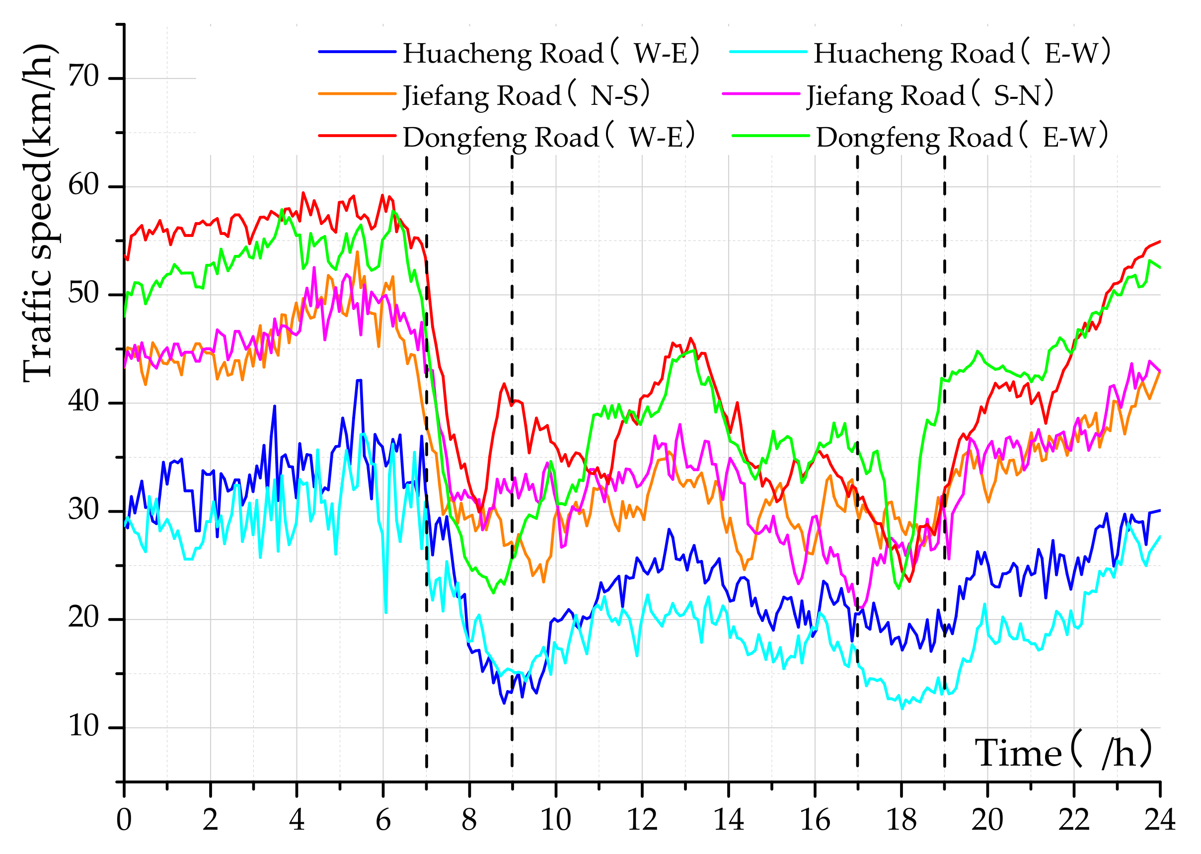
We have carried out a statistical analysis of the speed of 128 main roads in Guangzhou city on 6 April, and the speed change curves of some roads of the whole day (0:00–23:59) are shown in Figure 1.

Figure 1 reveals some laws, as follows:

• In different directions, the traffic speed of the same main road varies;
• The traffic speed trend of each section in one day is generally consistent, vehicles can pass freely during 19:00 to 07:00, however, traffic speed in rush hours (07:00–09:00, 17:00–19:00) obviously decreased, and the speeds at the non-peak time of the day (09:00–17:00) show obvious fluctuation.

After a number of days’ observation and analysis of traffic speed of these 128 main roads, we found that traffic speeds of each main road between 00:00 and 07:00 were stable, and could be described as a determined constant approximately. In order to simplify the calculation, we expressed the traffic speed of each main road by a piecewise function as follows.

$$v=\left\{\begin{array}{l}M,t\in [00:00,07:00)\\ f(t_1),t_1\in [07:00,09:00)\\ f(t_2),t_2\in [09:00,17:00)\\ f(t_3),t_3\in [17:00,19:00)\\ f(t_4),t_4\in [19:00,00:00)\end{array}\right.$$

(1)

2.2. Decision Factors of Vehicle Passable Speed

In actual road networks, the customer points i and j are hardly connected by a single path generally, there is more than one intermediate node in the route from i to j. Therefore, to get the average speed $v_{ij}$ between the customer i and the customer j, it is necessary to consider the actual traffic, and make clear the speed of the passage and the actual distance between the two nodes.

Based on historical speed data obtained from the intelligent transportation system, it is easily to calculate average speed of each section during a day. Furthermore, we can find the shortest path between i and j according to the distance and travel time $t_{ij}$ between the nodes in actual road networks. Average speed $v_{ij}$ of the vehicle in the route from i to j can be calculated as follows.

$$v_{ij}=\frac{d_{ij}}{t_{ij}}$$

(2)

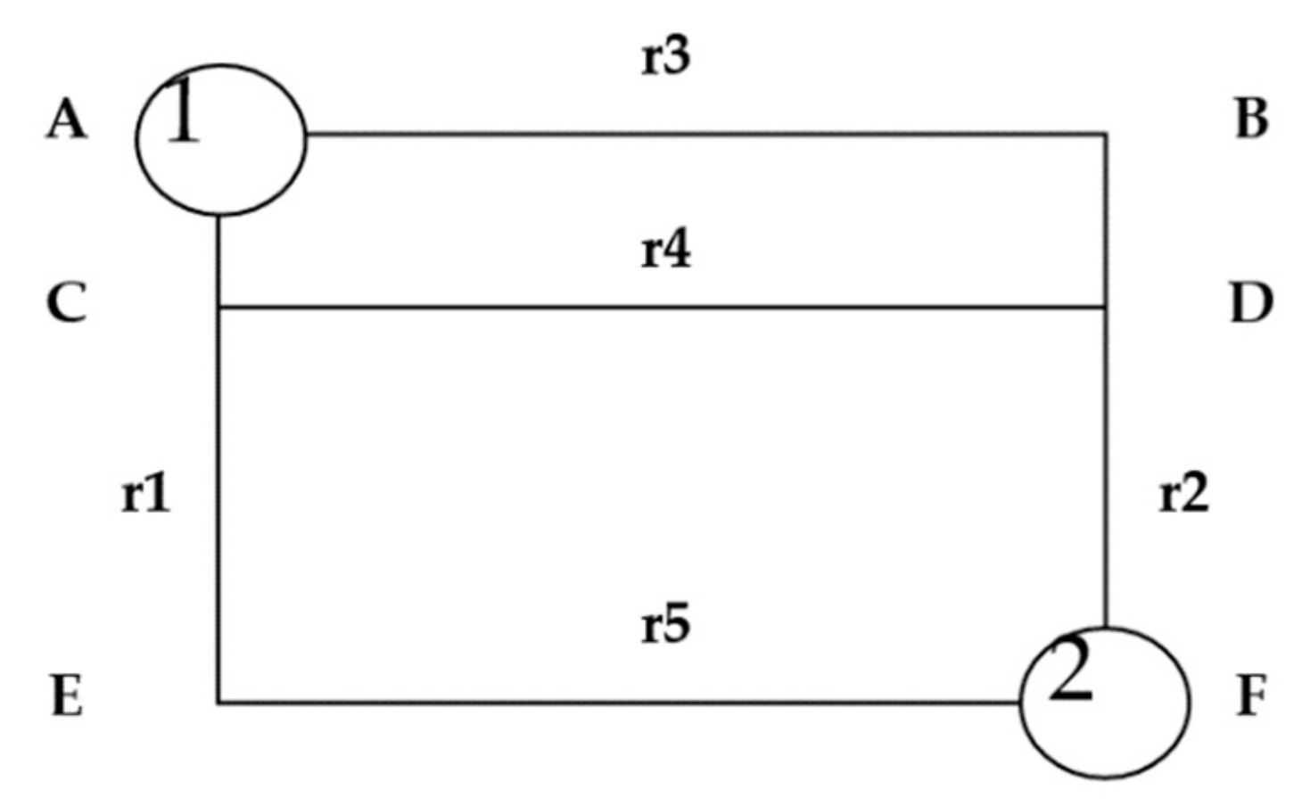
An example is given to further explain our method. As shown in Figure 2, during the driving process from the customer 1 (node A) to the customer 2 (node F), the vehicle may pass through the following road network. It is easy to see that that road network between node A and node F consists of many paths, of which both the historical traffic speed and the length are different.

To find the best and the fastest route from A to F, we can transfer this problem to a shortest path problem by calculating travel time on each road as shown in

Table 1. Traffic speed and length of roads 1 to 5.

Road	Direction	Average Historical Traffic Speed (km/h)	Length of the Road (km)	Travel Time (min)
r1	A–C	40	0.5	0.75
	C–E	40	1.0	1.5
r2	B–D	30	0.5	1
	D–F	30	1.0	2
r3	A–B	30	2.0	4
r4	C–D	50	2.0	2.4
r5	E–F	40	2.0	3

.

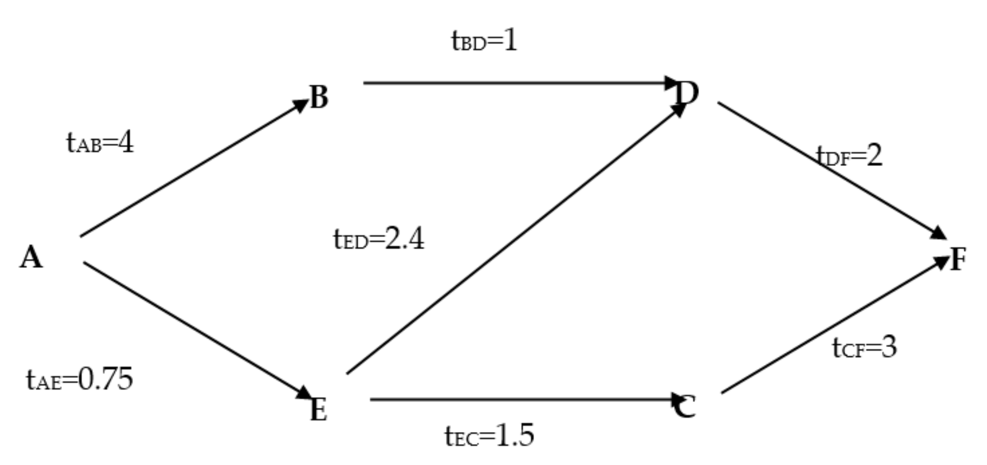
Figure 3 depicts the traffic network between A and F and the time (min) required to cross each road with a directed graph. The tool “QM for Windows” was employed in our method to find the best route from node A to node F. In this numerical example, the best route provided by the tool was A→C→D→F, the total time consumption was 5.15 min and the travel distance was AC + CD + DF = 1 + 2 + 1 = 4 km. Thus, the average speed of the vehicle which traveled from node 1 to node 2 can be calculated as $v_{12}=\frac{d_{12}}{t_{12}}=60\cdot \frac{4}{5.15}=46.6$ km/h.

The calculated average speed method (CASM) based on actual historical data of each road and the shortest path rule will be adopted in the following parts, meanwhile, the shortest travel time and the distance between node i and node j will be presented in a table. It is worth noting that the measurement of fuel consumption is based on the CAMS in later parts.

2.3. Assumptions and Basic Parameters

Foods like fruits and vegetables are different from ordinary foods. They are generally goods that need refrigeration. There are certain requirements for temperature in the distribution process. When the transportation conditions and requirements are inconsistent, the quality of the foods will probably decline or even be damaged, and with the increase of distribution time, the damage of foods will be aggravated. In the actual distribution process, this will also be affected by the external traffic environment. Especially in the city, the complexity of the road seriously restricts the distribution activities, so the goods in the distribution process show the characteristics of being perishable. Since a perishable foods delivery system is complex, some assumptions are proposed to model the delivery system:

(1)

The customers’ demands and information, including the number, the locations and time windows are known, as well as the number of refrigerator vehicles;

(2)

All the perishable foods are delivered by homogeneous refrigerator vehicles without taking deterioration into account;

(3)

The vehicles set off from the same distribution center and return back to the center finally;

(4)

The storage capacity of each refrigerator vehicle and the volume are limited, equal to or less than the capacity of the car;

(5)

Each customer node is serviced by only one refrigerator car without picking up products;

(6)

Some basic parameters and decision variables are presented in

Table 2. Basic parameters.

Symbol	Meaning	Symbol	Meaning
dij	distance between node i and node j	[ETi,LTi]	time window ordered by customer i
vij	average speed from customer i to customer j	xijk	binary variable, if refrigerator car k goes to node j after servicing node i, Xijk = 1, otherwise Xijk = 0
qi	quantity of perishable foods ordered by customer i	yik	binary variable, if node i is serviced by refrigerator car k, yijk = 1, otherwise yijk = 0
bi	average volume of perishable foods ordered by customer i	ue	penalty weight when a car arrives early
pi	average price of perishable foods ordered by customer i	ul	penalty weight when a car is delayed
gi	average weight of perishable foods ordered by customer i	si	service time at customer i
ti	arriving time at customer i	wij	weight of the products on the refrigerator car from node i to node j
N	number of the customers	tij	shipping time between node i and node j
Fij	carbon emissions of from node i to node j	Eij	unit fuel consumption from node i to node j

.

2.4. Cost Function Formulation

All costs incurred by refrigerator car from the distribution center to destination should be taken into account. Therefore, fixed cost, transportation cost, penalty cost and refrigeration cost are included in model I. Fixed cost is a sum of starting cost and maintenance cost for each vehicle, the transportation cost is related to fuel consumption and a penalty cost exists when the delivery time window is violated at the retailers. Finally, refrigerator cost is refrigeration cost for perishable food during the distribution.

(1)

Fixed cost

Fixed cost includes the starting costs of the refrigerator car, salaries paid for drivers, maintenance fee of the cars, road maintenance fee and annual check-up fees. Let $l_k$ denote the fixed cost of each car, the total fixed cost needed to be payed can be formulated as:

$$C_l={\displaystyle \sum _{k=1}^K{l}_k}.$$

(3)

(2)

Transportation cost

The transportation cost of perishable foods during the shipments is considered as fuel cost only, of which excellent linearity is found with transportation distance. The total transportation cost in the distribution is the fuel costs consumed by all vehicles, which is related to vehicle fuel consumption and unit fuel cost. Let denotes unit fuel price, the total transportation cost can be expressed as:

$$C_d={\displaystyle \sum _{k=1}^K{\displaystyle \sum _{i=0}^N{\displaystyle \sum _{j=0}^N{E}_{ij}}}}\cdot d_{ij}\cdot x_{ijk}\cdot f_k.$$

(4)

$E_{ij}$ is unit fuel consumption from node i to node j, $w_{ij}$ is weight of the products on the refrigerator car from node i to node j, more concretely, unit fuel consumption per kilometer is calculated as follows.

$$E_{ij}={\beta }_0+{\beta }_1{w}_{ij}+\frac{{\beta }_2}{v_{ij}^2}$$

(5)

${\beta }_0$ denotes unit fuel consumption when the car is empty, ${\beta }_1$ denotes influence factors on unit mileage fuel consumption of vehicle under extra load, ${\beta }_2$ denotes influence factors of vehicle speed on unit mileage fuel consumption.

(3)

Penalty cost

As for the penalty cost, since customers have high quality requirement for perishable food, penalty cost is charged when a retailer’s time window is violated. Penalty cost is related to price and quantity of products ordered by customers as well as the penalty weight $u_e$ when a car arrives early, $u_l$ when it is delayed ($u_e<u_l$).

Add up all penalties for all retailors whose time window is violated and the total penalty cost can be calculated as follows. The symbols and their definitions are listed in Table 2.

$$C_t={\displaystyle \sum _{k=1}^K{\displaystyle \sum _{i=0}^N{y}_{ik}}}{p}_i{q}_i[\max (E{T}_i-t_i,0)u_e+\max (t_i-L{T}_i,0)u_l]$$

(6)

(4)

Refrigeration cost

In this study, perishable food is delivered (distributed) by mechanical refrigerator car, which is common in Guangzhou, China. The refrigeration depends on refrigerants absorbing heat through evaporation. Hence, the refrigeration cost comes from the consumption of refrigerants in two courses as the car is on the road and unloading foods at the retailors’.

a.

Refrigeration cost in transportation

The refrigerating cost generated by a vehicle is determined by the amount of refrigerant consumed, which can be measured by thermal load generated by refrigerated cars in transportation. The thermal load generated by a refrigerator car during driving can be expressed as below.

$$G_{k1}=\mu S(1+\eta )(T_w-T_n)$$

(7)

The symbol $\mu$ denotes thermal conductivity ($kCal/h\cdot m^2\cdot C°$), S denotes the area irradiated by sun, which can be calculated as $S=\sqrt{S_w\cdot S_n}$, $S_w$ and $S_n$ are the external surface area and the internal surface area of the refrigerated car respectively. The symbol $\eta$ denotes deterioration factor of the carriage, $T_w$ denotes environmental temperature and $T_n$ denotes temperature in the carriage.

Each car departs from the distribution center, after completing the distribution tasks, it returns to the distribution center. The total time assumption can be measured as follows.

$$t_{total}={\displaystyle \sum _{i=0}^N{\displaystyle \sum _{j=0}^N(t_{ij}+s_j)x_{ijk}}}$$

(8)

Thus, the refrigeration cost in transportation is:

$$C_{q1}={\displaystyle \sum _{k=1}^K\lambda G_{k1}{t}_{total}=}{\displaystyle \sum }_{k=1}^K{\displaystyle \sum }_{i=0}^N{\displaystyle \sum }_{j=0}^N\lambda \mu S(1+\eta )(T_w-T_n)(t_{ij}+s_j)x_{ijk}$$

(9)

b.

Refrigeration cost in unloading foods

Once the vehicle arrives at a retailors’ grocery, it is inevitable to open the door to unload the foods ordered by the retailor. If the door is open, the outside air will be convective with the air in the car, accelerating the refrigerant consumption. The thermal load of vehicle k is:

$$G_{k2}=\delta (0.54V+3.22)(T_w-T_n)$$

(10)

where $V$ denotes the carriage volume of vehicle $k$, $\delta$ is a frequency coefficient of opening the door, when the door is opened one to five times, the value is 0.50, when opened between five and ten times, the value is 0.75 and $\delta$ equals to 1 once the door is opened more than ten times.

Thus, the refrigeration cost in unloading foods can be expressed as follows.

$$C_{q2}={\displaystyle \sum _{k=1}^K\sum _{i=0}^N\mathit{\lambda }{\mathit{G}}_{\mathit{k}2}{\mathit{s}}_{\mathit{i}}{\mathit{y}}_{\mathit{ik}}=}{\displaystyle \sum }_{\mathit{k}=1}^{\mathit{K}}{\displaystyle \sum }_{\mathit{i}=0}^{\mathit{N}}\mathit{\lambda }{\mathit{s}}_{\mathit{i}}{\mathit{y}}_{\mathit{ik}}\mathit{\delta }(0.54\mathit{V}+3.22)({\mathit{T}}_{\mathit{w}}-{\mathit{T}}_{\mathit{n}})$$

(11)

Therefore, the total refrigeration cost $C_q$ in the whole distribution can be expressed as:

$$\begin{array}{ll}{C}_q=C_{q1}+C_{q2}& ={\displaystyle \sum _{k=1}^K{\displaystyle \sum _{i=0}^N{\displaystyle \sum _{j=0}^N\lambda \mu S(1+\eta )(T_w-T_n)(t_{ij}+s_j)x_{ijk}}}}\\ & +{\displaystyle \sum _{k=1}^K{\displaystyle \sum _{i=0}^N\lambda s_i{y}_{ik}\delta (0.54V+3.22)(T_w-T_n)}}\end{array}$$

(12)

(5)

Carbon emission cost

To calculate the carbon emission cost in cold chain distribution, we need to calculate the amount of emissions generated in distribution. In this paper, the carbon emissions in the process of cold chain distribution are considered from two aspects: the emissions of the fuel consumption of the vehicle, and the other produced by the refrigeration equipment of the car.

The CO₂ emissions from fuel consumption during vehicle driving can be calculated through the fuel consumption and CO₂ emissions coefficient. According to the low carbon policy, carbon tax is used to quantify the carbon emissions in the distribution process. Therefore, the cost of carbon emissions is expressed as:

$$C_{c{o}_2}{}_1=a_{C{O}_2}\cdot m\cdot {\displaystyle \sum _{k=1}^K{\displaystyle \sum _{i=0}^N{\displaystyle \sum _{j=0}^N{E}_{ij}}}}\cdot d_{ij}\cdot x_{ijk}$$

(13)

The CO₂ emissions generated by refrigeration during the whole distribution are related to the distance and load weight of the car, this part of emissions $F_{ij}$ can be expressed as:

$$F_{ij}=\omega \cdot w_{ij}\cdot d_{ij}$$

(14)

It is noted that $\omega$ is unit carbon emissions when a refrigerator car carrying a unit of food travels per kilometer. Under the carbon tax policy, the total carbon emission cost is as follows:

$$C_{c{o}_2}{}_2=a_{C{O}_2}{\displaystyle \sum _{k=0}^K{\displaystyle \sum _{i=0}^N{\displaystyle \sum _{j=0}^N{F}_{ij}{x}_{ijk}}}}=a_{C{O}_2}\omega {\displaystyle \sum _{k=0}^K{\displaystyle \sum _{i=0}^N{\displaystyle \sum _{j=0}^N{w}_{ij}{d}_{ij}{x}_{ijk}}}}$$

(15)

Therefore, the carbon emission cost of fresh cold chain products in the whole distribution process is:

$$C_{C{O}_2}=C_{C{O}_{2}1}+C_{C{O}_{2}2}=a_{C{O}_2}({\displaystyle \sum _{k=1}^K{\displaystyle \sum _{i=0}^N{\displaystyle \sum _{j=0}^{N}m{E}_{ij}{d}_{ij}}}}{x}_{ijk}+{\displaystyle \sum _{k=1}^K{\displaystyle \sum _{i=0}^N{\displaystyle \sum _{j=0}^N\omega w_{ij}{d}_{ij}}}}{x}_{ijk})$$

(16)

2.5. Mathematical Model

This study deals with optimizing the delivery routes of a cold chain distribution center and demonstrates how carbon tax policy influences operation of the distribution center.

In order to make clear how carbon tax policy will affect distribution of the enterprise, two mathematical models were established to optimize the distribution routes. One (Model I) is a vehicle routing problem with time windows (VRPTW) model without low carbon factors and the other (Model II) takes carbon tax policy into account.

Both model I and model II were assumed to minimize cost, optimizing routes of each vehicle from the distribution center to each customer. At first, model I was established by considering fixed cost of the vehicles, transportation cost, (3) penalty cost and refrigerating cost. To further explore the influences of carbon tax policy, model II was devised by adding carbon tax generated during the distribution of the enterprise to the objective function of model I.

2.5.1. VRPTW Mathematical Model (Model I)

From the discussion above, a nonlinear programming problem is formulated as follows by minimizing the total cost in distribution.

$$\begin{array}{ll}\min Z& ={\displaystyle \sum _{k=1}^K{l}_k}+{\displaystyle \sum _{k=1}^K{\displaystyle \sum _{i=0}^N{\displaystyle \sum _{j=0}^N{E}_{ij}}}}{d}_{ij}{x}_{ijk}{f}_k+{\displaystyle \sum _{k=1}^K{\displaystyle \sum _{i=1}^N{y}_{ik}{p}_i{q}_i[\max (E{T}_i-t_i,0)u_e+\max (t_i-L{T}_i,0)u_l}}]\\ & +{\displaystyle \sum _{k=1}^K{\displaystyle \sum _{i=0}^N{\displaystyle \sum _{j=0}^N\lambda \mu S}}(1+\eta )(T_w-T_n)(t_{ij}+s_j)x_{ijk}+}{\displaystyle \sum _{k=1}^K{\displaystyle \sum _{i=0}^n\lambda s_i{y}_{ik}\delta }}(0.54V+3.22)(T_w-T_n)\end{array}$$

(17)

such that

$${\displaystyle \sum _{i=1}^N{q}_i{g}_i{y}_{ki}\le W,k=1,2,3...K},$$

(18)

$${\displaystyle \sum _{i=1}^N{q}_i{b}_i{y}_{ki}\le V,k=1,2,3...K},$$

(19)

$$E_{ij}={\beta }_0+{\beta }_1{w}_{ij}+\frac{{\beta }_2}{v_{ij}^2},$$

(20)

$$w_{ij}={\displaystyle \sum _{i=1}^N{q}_i}{g}_i{y}_{ki}-{\displaystyle \sum _{i=1}^i{q}_i}{g}_i{y}_{ki},k=1,2,...K,$$

(21)

$$t_0=0$$

(22)

$$t_i+s_i+t_{ij}-M(1-{\displaystyle \sum _{k=1}^K{x}_{ijk}})\le t_j,i,j=1,2,...N,andi\ne j,$$

(23)

$$v_{ij}=\frac{d_{ij}}{t_{ij}},i,j=1,2,...N,andi\ne j,$$

(24)

$${\displaystyle \sum _{k=1}^K{\displaystyle \sum _{i=0}^N{x}_{ijk}}}=1,j=1,2,...N,$$

(25)

$${\displaystyle \sum _{k=1}^K{\displaystyle \sum _{j=0}^N{x}_{ijk}}}=1,i=1,2,...N,$$

(26)

$${\displaystyle \sum _{k=1}^K{y}_{ki}}=1,i=1,2,...N.$$

(27)

To make the model more practical, the maximum cargo capacity of refrigerator car was considered, as well as both customers’ time windows and refrigeration cost during the delivery.

Equation (17) represents the total cost of distribution, including fixed cost, transportation cost, penalty cost and refrigeration cost.

Constraint (18) restricts that the total amount on each refrigerator car are limited by the capacity, while constraint (19) restricts the total volume.

Equation (20) expresses the calculation of unit fuel consumption.

Equation (21) represents the weight on the car during the trip from node i to node j.

Equation (22) and constraint (23) represent temporal continuity.

Equation (24) represents the calculated average speed between node i and node j.

Equations (25) and (26) ensure that all customers are serviced

Equation (27) expresses that each customer is serviced by only one refrigerator car.

2.5.2. Mathematical Model Considering Carbon Emissions (Model II)

With the elevated level of public and organizational awareness about sustainability and global climate, the adoption of environmentally conscious practices are taken into consideration in the management of cold chain distributions. Hence, classical VRPTW models aiming to minimize cost are no longer appropriate enough to cope with this emerging and pressing issue. In this part, a model, namely, the model II, was formulated to explore how carbon emission policy affects the operational cost of the cold chain distribution. In this model, the impact of carbon emission policy are assessed in a form of carbon taxes. In addition, model II is an improved version of model I, but the constraints remains the same.

$$\begin{array}{ll}\min Z& ={\displaystyle \sum _{k=1}^K{l}_k}+{\displaystyle \sum _{k=1}^K{\displaystyle \sum _{i=0}^N{\displaystyle \sum _{j=0}^N{E}_{ij}}}}{d}_{ij}{x}_{ijk}{f}_k+{\displaystyle \sum _{k=1}^K{\displaystyle \sum _{i=1}^N{y}_{ik}{p}_i{q}_i[\max (E{T}_i-t_i,0)u_e+\max (t_i-L{T}_i,0)u_l}}]\\ & +{\displaystyle \sum _{k=1}^K{\displaystyle \sum _{i=0}^N{\displaystyle \sum _{j=0}^N\lambda \mu S}}(1+\eta )(T_w-T_n)(t_{ij}+s_j)x_{ijk}+}{\displaystyle \sum _{k=1}^K{\displaystyle \sum _{i=0}^n\lambda s_i{y}_{ik}\delta }}(0.54V+3.22)(T_w-T_n)\\ & a_{C{O}_2}({\displaystyle \sum _{k=1}^K{\displaystyle \sum _{i=0}^N{\displaystyle \sum _{j=0}^{N}m{E}_{ij}{d}_{ij}}}}{x}_{ijk}+{\displaystyle \sum _{k=1}^K{\displaystyle \sum _{i=0}^N{\displaystyle \sum _{j=0}^N\omega w_{ij}{d}_{ij}}}}{x}_{ijk})\end{array}$$

(28)

3. Solution Algorithm

The VRPTW is inherently an NP-hard(non-deterministic polynomial) problem [1], flexible time windows and complex cost functions make the perishable food delivery problem even more challenging. A hybrid algorithm (GATS) combines genetic algorithm (GA) and tabu search algorithm (TS) is adopted in this study, the GA is designed for global searching while TS is for local search.

After generating the initial population, selection, crossover and mutation operation are conducted. Then, to avoid falling into local optimal solution, tabu search is employed for further optimization. The optimized chromosome is selected by the evaluation function. The hybrid algorithm (GATS) for model I and model II was designed in eight steps as follows.

Step 1. Generate the initial population of N chromosomes.

Step 2. Formulate the evaluation function and evaluate the fitness of each chromosome in the population.

Step 3. Update the population by repeating the following steps.

1.

[Selection] Select two parent chromosomes by roulette choosing method, from the current population;

2.

[Crossover] The crossover of chromosomes is carried out by a partial cross rule, as exchanging a fragment of the same length and position in two chromosomes;

3.

[Mutation] The uniform mutation method is adopted for mutation. Some genes are to be selected randomly and replaced by random number between 0 and 1;

4.

[Accepting] Accept the offspring generated in mutations, and save the offspring in a new population;

5.

[Update] Update the previous population by replacing the old one with the newly-generated population.

Step 4. Once the number of iterations reaches a certain number, stop, record the better solution, else back to Step 3.

Step 5. Tabu search for the best solution. The search scope is the neighborhood of the better solution.

The details for GATS are described below.

There are dozens of customer points and vehicles involved in the problem, the constraints of load and volume of vehicle also must be satisfied, so each chromosome is encoded with random key in Step 1. These chromosomes denote different delivery solutions, which can be decoded as actual routes of the vehicles. The distribution center owns K vehicles and services for N customer points. Due to the actual constraint conditions such as vehicle load and retailors’ time window, many vehicles need to be arranged, thus many sub-paths will be created. The random key encoding dimension of the problem is (N + K − 1), each dimension consists of N decimals between 0 and 1. To decode the vehicle routes, we need to arrange these N decimals (also genes) in order of small to large, then, the sequence of the genes is the visiting order of the retailors of a specific vehicle. Note that sub-path segmentation node is adopted to separate the route of different vehicles; the nodes are assigned a value between (N − 1) to (N + K − 1). A chromosome example is given as follows.

Suppose N = 10, K = 3, the encoding dimension is $(10+3-1)\times 1=12\times 1$, thus a possible encoding can be (0.12, 0.37, 0.22, 0.96, 0.56, 0.35, 0.76, 0.57, 0.38, 0.91, 0.71, 0.26). Using the random key decoding rule, it is easy to get the integer arrangement (1, 5, 2, 12, 7, 4, 10, 8, 6, 11, 9, 3). The integers 11 and 12 are the so-called sub-path segmentation, and the vehicle routes are:

Route No. 1 is 0→1→5→2→0

Route No. 2 is 0→7→4→10→8→6→0

Route No. 3 is 0→9→3→0.

As for initial population, each chromosome is formed using the random key decoding rule, and the total number of chromosomes in this paper is set as nPop = 50. Given that the constraints of vehicle loading weight and volume limitation, the evaluation function of each chromosome is formulated as the sum of the objective function and the penalty value violating the constraints. The objective function of the models are to minimize the total cost, if the evaluation function value of a chromosome is smaller, it is more likely to be selected, which also represents better distribution scheme. Let f(x) express the evaluation function value of chromosome x, let the symbol Z_x represents the objective function value of chromosome x, and θ represents the penalty coefficient. Therefore, the evaluation function can be described as $f(x)=Z_x+\Delta \cdot \theta$. Using the roulette choosing method, a population is selected to find an optimal solution. To achieve high performances of GA, it is important to pass the useful traits down to the offspring. Reproduction, which consists of crossover and mutation, is a crucial mechanism to maintain adaptability of the population. The crossover process is conducted utilizing partial cross rule, specifically, exchanging a fragment of the same length and position in two chromosomes:

Parent 1: 0.12 0.25 0.73 0.27 0.87 0.64 0.87 0.45 0.78

Parent 2: 0.25 0.67 0.26 0.98 0.72 0.65 0.22 0.72 0.68

Offspring 1: 0.12 0.25 0.26 0.98 0.72 0.64 0.87 0.45 0.78

Offspring 2: 0.25 0.67 0.73 0.27 0.87 0.65 0.22 0.72 0.68

The underlined fragments of the parents have been swapped to generate offspring1 and 2.

Mutation is important in biological evolution, and can potentially generate new adaptable genes. In GA, mutation operation can expand the search space of feasible solutions, avoiding premature convergence and increasing the probability of obtaining the optimal solution. In this paper, the uniform mutation method was adopted, namely, selecting some genes of a chromosome randomly and replacing them with random numbers between 0 and 1. For example, if a chromosome is encoded as (0.12, 0.89, 0.78, 0.25, 0.67, 0.77, 0.82), during the mutation, the gene “0.77” is replaced by the random number “0.28”, so the chromosome is updated as (0.12, 0.89, 0.78, 0.25, 0.67, 0.28, 0.82).

In step 5, further optimization on the basis of better solutions provided by GA is conducted in tabu search. The tabu table is designed at first for tabu search. After tabu search, new solutions are generated, so updating both the currently best-so-far solution and the candidate solution set. If the end condition is met, namely, the iteration number reaches 300, the best-so-far solution is output as the optimal solution, otherwise the tabu search is continued.

4. Computation Example

4.1. Data Source

The data of the operation are collected from the transaction data of an enterprise. Enterprise A is a fruit and vegetable production, processing and operation enterprise. It has a large fruit and vegetable base in major cities throughout China to supply fresh fruits and vegetables to customers. Since all products of enterprise A are organic food, it is important to ensure the freshness of the products through the picking, processing and packing. Thus, products from distribution center to the retailors are to be delivered through continuous cold chain logistics. Based on the customer demand data of distribution center of enterprise A in a certain period of time, this paper takes the typical data as the case study data. The enterprise A owns a cold chain warehouse, which is also known as a distribution center in Guangzhou. One day, it received orders from 10 retailors (large chain supermarkets) in Guangzhou. Due to the restriction of urban delivery time and to meet the customers’ demands, the distribution center starts distributions at 04:00. Generally, at the same time, all those distribution tasks are completed before 06:00. The case is based on the actual geographical location of each node in the map. In order to describe the location accurately, the case is expressed in the form of coordinate system, in which the coordinate position of distribution center is (15, 2). The ten retailors’ demands and the locations are listed in

Table 3. Retailors’ demand and basic information.

Retailor i	Location	Ordered Quantity qi	Average Weight gi	Average Volume bi	Average Price pi	Time Window [ETi,LTi] (h2)	Service Time si (h2)
1	(26, 2)	2900	0.3379	0.0013	3.3103	[0.00, 0.50]	0.1
2	(33, 7)	4200	0.3214	0.0016	3.3810	[0.25, 0.75]	0.1
3	(22, 26)	3500	0.5129	0.0022	6.8000	[0.33, 0.75]	0.1
4	(9, 32)	2900	0.5000	0.0023	5.6207	[0.75, 1.25]	0.1
5	(27, 33)	2600	0.4385	0.0030	5.7692	[0.33, 1.25]	0.1
6	(49, 34)	2800	0.5000	0.0029	6.0714	[1.33, 2.00]	0.1
7	(43, 38)	2000	0.3500	0.0020	4.5000	[1.25, 1.75]	0.1
8	(34, 45)	4200	0.2286	0.0023	2.2857	[1.25, 2.00]	0.1
9	(22, 43)	3800	0.4474	0.0017	4.4211	[1.50, 2.00]	0.1
10	(10, 43)	2600	0.4231	0.0030	4.8462	[0.75, 2.00]	0.1

.

After knowing the geographical location of the distribution center and the demand point, based on the historical traffic information of the section obtained by the Guangzhou Intelligent Transportation System, the shortest traveling time and the shortest distance (See Appendix A) can be calculated by the shortest path calculation method introduced above.

Note that, the enterprise A has signed a distribution service contract with all ten retailors to provide high quality service for them. Once the time window of a retailor is violated, then the penalty cost is charged at a 0.05 percentage of the ordered price. The refrigerator cars are to unload the foods at the retailors, and the unloading takes about 6 min estimated on the basis of our survey.

In addition to the above information about the retailers, some necessary parameters in this computation example are listed in

Table 4. Necessary parameters and the value in the computation example.

Parameter	Meaning	Value
	number of the customers	10
	number of vehicles available in distribution centers	4
	fixed cost of each car	300
	maximum load of vehicle	3750 kg
	the carriage volume of vehicle	20.664 m3
	penalty weight when a car arrives early	0.05%
	penalty weight when a car is delayed	0.05%
	service time at customer i	0.1 h
	unit fuel consumption when the car is empty	0.3 L
	influence factors on unit mileage fuel consumption of vehicle under extra load	8 × 10−5
	influence factors of vehicle speed on unit mileage fuel consumption	200
	unit fuel price	5.6 RMB/L
aCO2	Unit carbon emission cost	0.125 RMB/kg CO2
m	carbon emissions coefficient of vehicle fuel	2.778 kg CO2/L
λ	unit refrigeration cost	1.5 RMB
η	deterioration of refrigerator car	0.08
μ	thermal conductivity	0.249 kCal/(h·m2·℃)
Sw	external surface area of refrigerated vehicle	95.57 m2
Sn	internal surface area of refrigerated vehicle	49.02 m2
S	area of refrigerated vehicle exposed to solar radiation	68.45 m2
Tw	outside temperature	20 ℃
Tn	temperature in the carriage	4 ℃
δ	frequency coefficient of opening the door	0.5
ω	carbon emissions from refrigeration by distributing unit weight goods per unit distance	0.0066

. Data were mainly provided by enterprises and queried by networks, and the relevant data of diesel fuel were collected from Guangzhou Oil Price Inquiry Network and International General Formula and Coefficient for Calculating Carbon Emissions.

4.2. Main Calculation Process

4.2.1. Operational Results of Urban Distribution Routing Optimization Model

MATLAB 2014a was used to program GATS. According to the actual operation and related literature, the relevant parameters were set. Among them, the population size was 50, the maximum number of iterations was 300, the crossover probability was 0.7, and the mutation probability was 0.03.

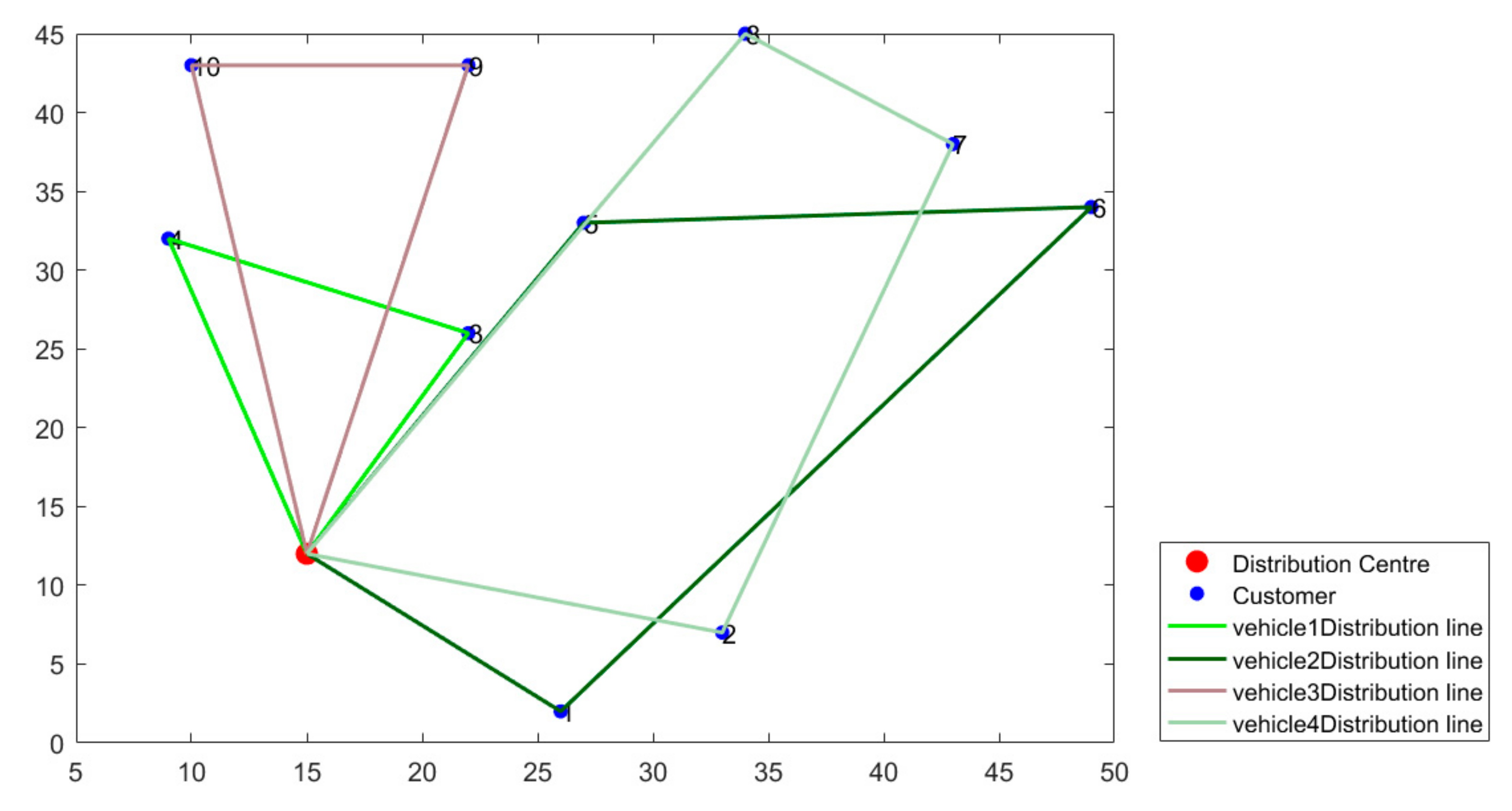
For the model without considering the low-carbon factors, using GATS in the process of solving, we can see that the model tended to be stable after 143 iterations and no better solution was found in the next 300 iterations. The minimum cost was 5318.60 RMB. By solving the model, the optimal distribution scheme was obtained. There were four distribution routes and four refrigerated vehicles are needed to complete the task. The distribution routes and delivery sequence are shown in Figure 4.

Route No.1 is 0→3→4→0;

Route No.2 is 0→1→6→5→0;

Route No.3 is 0→9→10→0;

Route No.4 is 0→8→7→2→0.

The specific costs are shown in

Table 5. The cost of model I solution (RMB).

Route	Fixed Cost	Transportation Cost	Refrigeration Cost	Penalty Cost	Summary
No.1	300	213.51	529.27	46.04	1088.82
No.2	300	293.30	891.10	36.00	1520.40
No.3	300	266.93	617.63	27.60	1212.16
No.4	300	372.87	802.75	21.60	1497.22
Summary	1200	1146.61	2840.74	131.24	5318.60

.

4.2.2. Operational Results of Urban Distribution Routing Optimization Model Considering Carbon Emissions

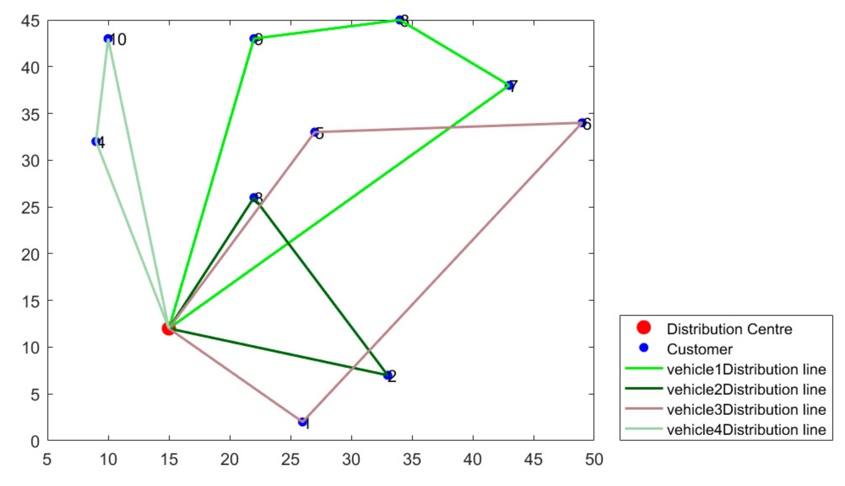
For the model considering the low-carbon factors, using GATS in the process of solving, we can see that the model tended to be stable after 107 iterations and no better solution was found in the next 300 iterations. The minimum cost is 5614.85 RMB. By solving the model, the optimal distribution scheme was obtained. There were four distribution routes and four refrigerated vehicles were needed to complete the task. The distribution routes and delivery sequence are shown in Figure 5.

Route No.1 is 0→9→8→7→0;

Route No.2 is 0→2→3→0;

Route No.3 is 0→1→6→5→0;

Route No.4 is 0→4→10→0.

The specific costs are shown in

Table 6. The cost of model II solution (RMB).

Route	Fixed Cost	Transportation Cost	Refrigeration Cost	Penalty Cost	Carbon Emissions Cost	Summary
No. 1	300	453.31	816.00	43.76	104.67	1717.74
No. 2	300	196.81	485.10	38.13	61.11	1081.15
No. 3	300	293.30	891.10	28.09	106.76	1619.25
No. 4	300	244.85	573.45	21.41	57.01	1196.72
Summary	1200	1188.27	2765.65	131.38	329.56	5614.85

.

5. Results and Discussion

5.1. Comparison Analysis of the Two Models

In this part, the operation results of the two models are compared from the three aspects of cost structure, carbon emissions and social benefits to explore the impact of low-carbon policy on the urban distribution path planning of enterprises.

Table 7. Comparison of cost structure and social benefits of two models.

Model	Fixed Cost (RMB)	Transportation Cost (RMB)	Refrigeration Cost (RMB)	Penalty Cost (RMB)	Carbon Emissions Cost (RMB)		Total Cost (RMB)	Carbon Emissions (kg)
					Social Payment	Enterprise Payment
I	1200	1146.61	2840.74	131.24	359.55	0.00	5678.14	2876.40
II	1200	1188.27	2765.65	131.38	0.00	329.56	5614.85	2636.48

shows the comparison of cost structure and social benefits of two models.

The costs in the two models can be clearly seen in Table 7. According to the total cost paid by the enterprise, the model I does not consider the low-carbon policy to optimize the route. The cost that the enterprise needs to pay included: fixed cost 1200 RMB, transportation cost 1146.61 RMB, refrigeration cost 2840.74 RMB and penalty cost 131.24 RMB. The minimum total cost of distribution was 5318.60 RMB. In model II, the route was optimized on the basis of low carbon policy. The total cost paid by the enterprise included: fixed cost 1200 RMB, transportation cost 1188.27 RMB, refrigeration cost 2765.65 RMB, penalty cost 131.38 RMB and carbon tax cost 329.56 RMB. The minimum total cost of distribution was 5614.85 RMB. According to the total cost paid by enterprises and society, in model I, the cost of carbon tax paid by the society was 359.55 RMB, and the total cost to enterprises and society was 5678.14 RMB. Model II considered the cost of carbon tax and optimized the route. The total cost paid by enterprises included the cost of carbon tax. The total cost to enterprises and society was 5614.85 RMB, 63.29 RMB less than the model I. Therefore, when enterprises plan urban distribution routes, low-carbon policy taken into account will result in lower total cost to enterprises and society, and the distribution scheme for enterprises and society is better.

Due to the importance of emission reduction in urban distribution to the global environment, the optimization of distribution routes is not only concerned with cost savings but also with carbon emissions. After calculation, from the perspective of carbon emissions, the total carbon emissions generated by the distribution scheme of model I was 2876.40 kg, while the distribution scheme of model II was 2636.48 kg, which was 239.92 kg less than that of model I. The reduction effect of carbon emissions in model II is obvious.

From the analysis of cost structure and carbon emissions, the model considering carbon emissions not only reduces certain carbon emissions, but also reduces the cost of carbon emissions that were originally paid by society. It means that the model has certain social benefits. From Table 7, the social benefits of the two models from the impact of corporate and social costs and carbon emissions can be further compared and analyzed.

Although the total cost paid by enterprises does not include carbon tax cost in the model I, the carbon emissions in distribution are real. The carbon emissions were 2876.40 kg, and the carbon tax cost is borne by the society. The cost of carbon tax paid by the society was 359.55 RMB. Model II considered the cost of carbon tax and optimized the route. The cost of carbon tax was added to the total cost of enterprise payment, and the enterprise bore the responsibility of paying carbon emissions. As shown in Table 7, the total cost to enterprise and society was reduced by 63.29 RMB compared with model I, and the carbon emissions were also reduced by 239.92 kg. This model achieved greater social benefits at a lower cost and was conducive to the common sustainable development of enterprises and society.

In summary, from the comparison of the above two models, the model considering carbon emissions is better than the model without considering carbon emissions when planning the optimal route of urban distribution for perishable foods. Not only is the total cost to enterprises and society better, but also the carbon emissions are smaller. For perishable foods, because of the special demand for temperature in urban distribution, refrigerated vehicles are mainly used for transportation. At the same time, it is necessary to meet customer demand time window to ensure service level. Carbon emissions in the process of distribution mainly come from the fuel combustion of vehicles and the refrigeration links. Therefore, in the process of distribution route planning, the factors such as vehicle refrigeration, time window, carbon emissions should be considered comprehensively to reduce carbon emissions in distribution, ensure customer service level, and maximize the benefits of enterprises and society under the carbon tax policy.

In addition, it is concluded that the model considering carbon emissions (model II) is better than the model not considering carbon emissions (modelI) in the optimal path planning. Not only is the distribution scheme obtained better in terms of the total cost to enterprises and society, but also the carbon emissions are lower. Model II achieves greater overall social benefits with less cost and is conducive to the common sustainable development of enterprises and society. Therefore, enterprises need to plan their routes on the basis of considering the low-carbon policy, which is not only conducive to enterprises choosing better distribution routes and reducing the total cost to enterprises and society, but also is a positive response to the national low-carbon policy to achieve the reduction of carbon emissions of the entire urban distribution industry.

5.2. Impact of Carbon Tax on Low Carbon VRP

At the end of 2016, China promulgated Environmental Protection Tax Law, which levies a carbon tax on atmospheric pollutants from 2018. Generally speaking, the higher the price of carbon tax, the more emissions will be reduced, but the economic burden will be heavier. In the case study above, it assumed that the unit cost of carbon emissions is 0.125 RMB/kg CO₂ according to the carbon tax policy. By adjusting the unit cost of carbon emissions, the impact on cost can be further analyzed. In order to get the further conclusion, this paper calculated the cost and carbon emissions when the unit carbon emissions cost is 0.05, 0.25, 0.50, 0.75, 1.00, 1.25 and 1.5. In addition, it calculated the optimal solution under the unit carbon emission cost through the GATS algorithm.

In order to obtain effective experimental results and further verify the validity of the results in the above case, this paper tests the stability of the algorithm first. In this paper, the example under each price of carbon tax was run independently 10 times.

Table 8. Stability analysis of genetic algorithm and tabu search hybrid algorithm (GATS).

Model	${\mathit{a}}_{\mathit{C}{\mathit{O}}_2}$	Best Solution	Mean	Standard Deviation	c.v	Relative Disparity
model I	0.05	5423.24	5460.67	41.44	0.76%	0.69%
	0.25	5939.11	6003.47	66.98	1.12%	1.08%
	0.5	6598.98	6697.74	92.40	1.38%	1.50%
	0.75	7258.10	7343.57	69.44	0.95%	1.18%
	1	7916.48	8085.24	157.83	1.95%	2.13%
	1.25	8576.34	8745.81	183.67	2.10%	1.98%
model II	0.05	5411.66	5458.26	53.90	0.99%	0.86%
	0.25	5938.96	5963.61	35.60	0.60%	0.42%
	0.5	6596.98	6645.99	60.79	0.91%	0.74%
	0.75	7233.01	7263.81	43.68	0.60%	0.43%
	1	7839.54	7904.47	72.37	0.92%	0.83%
	1.25	8445.67	8494.81	41.64	0.49%	0.58%
average	-	-	-	-	1.06%	1.03%

shows the best solution, mean, standard deviation, coefficient of variance (C.V), and the relative gap between the mean and the best solution (relative disparity). Among them, C.V = standard deviation/mean, relative disparity = (mean − best solution)/best solution.

Table 8 shows that: (1) the volatility of the solution is small, the coefficient of variance is controlled within 2.10%, and the average coefficient of variance of all examples is 1.06%; (2) the relative disparity between the mean and the best solution is small, controlled within 2.13%, and the average value of the relative disparity of all examples is 1.03%. Thus, the stability of this algorithm is high.

Because the algorithm had good stability, this paper chose the mean value of ten operations as the result of examples to analyze the impact of carbon tax on low carbon VRP. Using the same method as the results analysis in the previous section, this part compares the cost structure and social benefits of the two models based on the calculation results of the two models under different unit carbon emission costs. The results are shown in

Table 9. Comparison of cost structure and social benefits of two models under different unit cost of carbon emissions.

Model	${\mathit{a}}_{\mathit{C}{\mathit{O}}_2}$	Fixed Cost (RMB)	Transportation Cost (RMB)	Refrigeration Cost (RMB)	Penalty Cost (RMB)	Carbon Emissions Cost (RMB)		Total Cost (RMB)	Carbon Emissions (kg)
						Social Payment	Enterprise Payment
model I	0.05	1200	1168.22	2817.49	131.53	143.43	0.00	5460.67	2868.6
	0.25	1200	1175.70	2798.49	133.16	696.11	0.00	6003.47	2784.4
	0.50	1200	1182.63	2798.05	129.42	1387.64	0.00	6697.74	2775.3
	0.75	1200	1193.88	2759.18	134.48	2056.03	0.00	7343.57	2741.4
	1.00	1200	1178.34	2786.57	132.86	2787.47	0.00	8085.24	2787.5
	1.25	1200	1176.14	2792.31	132.14	3445.22	0.00	8745.81	2756.2
model II	0.05	1200	1174.49	2816.89	131.88	0.00	135.00	5458.26	2700.0
	0.25	1200	1184.87	2782.87	133.62	0.00	662.25	5963.61	2649.0
	0.50	1200	1195.74	2827.93	135.40	0.00	1286.91	6645.99	2573.8
	0.75	1200	1270.16	2834.12	131.40	0.00	1828.13	7263.81	2437.5
	1.00	1200	1241.00	2846.93	133.29	0.00	2483.25	7904.47	2483.3
	1.25	1200	1216.10	2863.72	132.70	0.00	3082.29	8494.81	2465.8

.

Table 9 details the cost structure of model I and model II under different unit cost of carbon emissions. It can be clearly seen that unit cost of carbon emissions has a certain impact on all costs except fixed costs, especially on the cost of carbon emissions. With the increase of unit cost of carbon emissions, the cost of carbon emissions will increase, which will lead to the increase of total cost. Meanwhile, Table 9 details the social benefits of model I and model II under different unit cost of carbon emissions. As discussed in the previous section, the model considering carbon emissions (model II) reduces social expenditure on environmental impacts while reducing carbon emissions. It shows that adjusting the unit price of carbon emissions also has a certain impact on the control of emissions while affecting costs, but it should be noted that this effect is not a simple linear relationship. 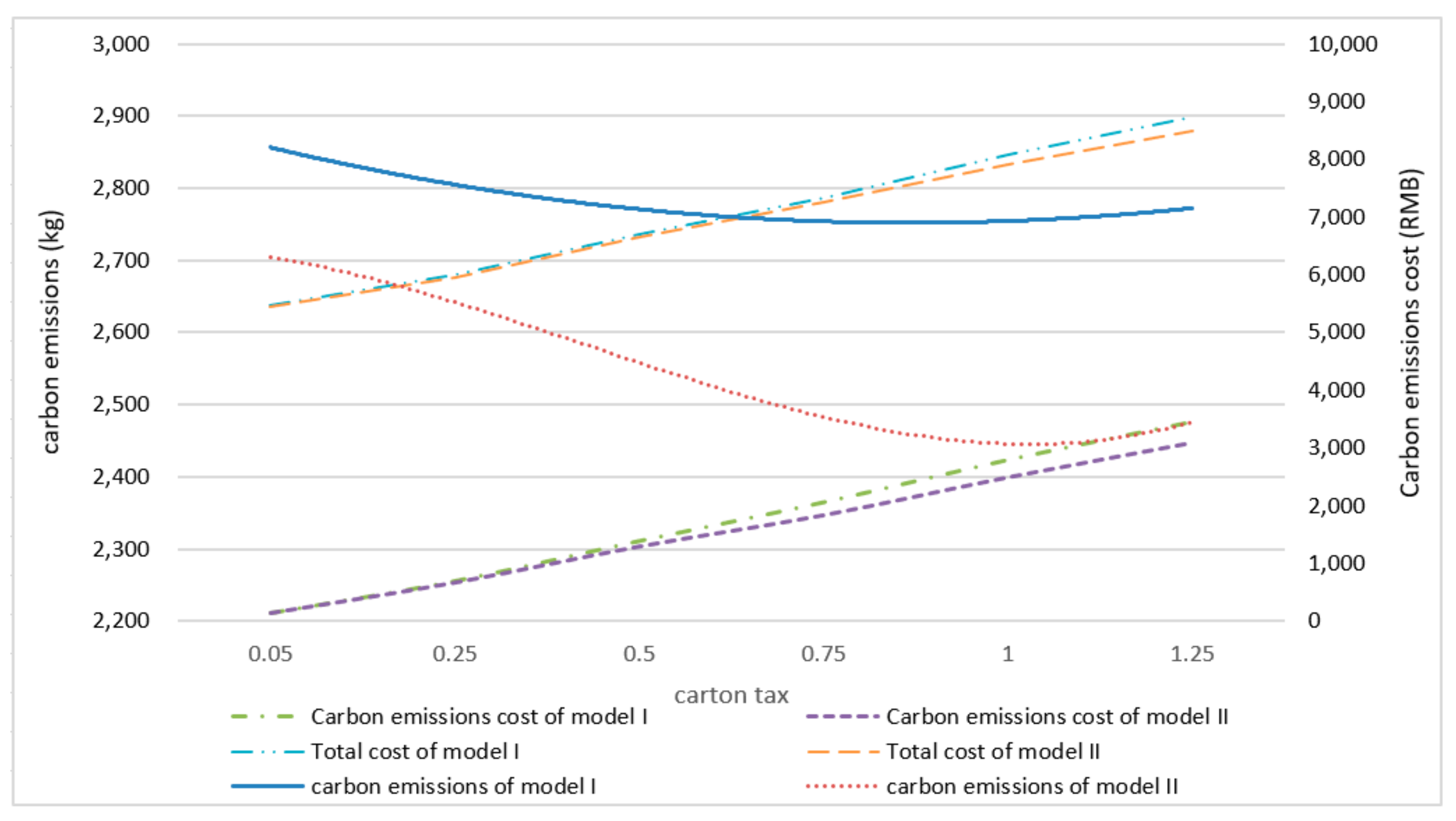The change curves showed in the Figure 6 can be obtained by observing its change.

Firstly, we can see that the trend of carbon emission cost is the same as the total cost paid by enterprises and society. This shows that carbon emission cost is a very important part of the total cost of low-carbon distribution. Taking the cost of carbon emissions as one of the costs when optimizing distribution routes can reduce the cost and the carbon emissions, and bring higher economic and social benefits. It further verifies the validity of the research conclusions. Secondly, from the perspective of the impact of carbon tax price on carbon emissions, the growth of carbon tax price can improve the low-carbon awareness of enterprises, make enterprises pay attention to the control of carbon emissions, optimize low-carbon distribution, and then achieve social energy conservation and emission reduction. However, as can be seen from the figure, it is not necessarily true that the higher the carbon tax price, the better effect of the carbon emission reduction. With the increase of the price of carbon tax, carbon emissions show a trend of decreasing gradually to a certain point and then rising, especially in model II. This is because beyond this point, the high carbon tax price brings a high cost of carbon emissions, and reduces the effect of VRP. Although the higher cost of carbon emissions can reduce carbon emissions to an extent, a higher carbon emission cost will not inevitably lead to more reduction of carbon emissions. Therefore, the government should set a reasonable carbon tax.

6. Conclusions

Based on the low-carbon policy, this paper analyzes the various cost components of urban distribution for perishable foods and the corresponding constraints, and builds a model of low-carbon urban distribution path optimization. A case study of a real enterprise data is conducted to explore the impact of low-carbon policies on urban distribution route planning for perishable foods. It is concluded that the model considering carbon emissions (model II) is better than the model not considering carbon emissions (model I) in the optimal path planning. Not only is the distribution scheme obtained better in the total cost to enterprises and society, but also the carbon emissions are lower. Model II achieves greater overall social benefits with less cost and is conducive to the common sustainable development of enterprises and society. The main research work of this paper is summarized as follows.

Historical traffic information on the actual road network has an important value for path planning. For the processing of distance between customer points, the traditional calculation method only considers the spatial straight line distance between two customer points, which will cause a certain deviation from reality. At the same time, the processing of vehicle speed generally assumes that the vehicle runs at a uniform speed, ignoring the impact of real-time traffic conditions on vehicle speed in the road network, which makes the optimization scheme lose practical significance. However, the study of distribution path optimization in this paper is based on the actual urban intelligent transportation system. According to the actual road network distribution and the distance between the nodes, the shortest path calculation method can be used to calculate the shortest travel time of any two nodes, so as to determine the shortest travel route and distance between the nodes.

Considering the low-carbon policy is very meaningful for the planning of urban distribution routes for perishable foods. Firstly, for enterprises, after the implementation of the carbon tax policy, the carbon emissions generated by urban distribution will be borne by the previous social commitments to the corresponding enterprises, and the carbon dioxide generated by the enterprises in the operation process will be converted into the economic costs of the enterprises. Therefore, perishable foods need to be routed on the basis of considering low-carbon policies when conducting urban distribution. This will not only help enterprises to choose better distribution routes, but also reduce the total cost to enterprises and society. It is also a positive response to the national low-carbon policy, which is conducive to the reduction of carbon emissions in the entire urban distribution industry. At the same time, for the society, under the carbon tax policy, the carbon emissions generated by urban distribution are converted into the economic costs of the corresponding enterprises, which can effectively encourage enterprises to strengthen the reduction of carbon emissions in urban distribution and achieve greater social benefits. It is suggested that government departments should give appropriate carbon tax subsidies or preferential tax policies to enterprises that implement low-carbon distribution, in order to improve the enthusiasm of enterprises to reduce emissions, promote the development of low-carbon urban distribution, and achieve win-win solutions between enterprises and society.

Therefore, enterprises need to plan their routes on the basis of considering the low-carbon policy, which is not only conducive to enterprises choosing better distribution routes and reducing the total cost to enterprises and society, but also a positive response to the national low-carbon policy to achieve the reduction in carbon emissions of the entire urban distribution industry. In addition, the price of carbon tax will have an impact on low-carbon distribution. Appropriate increase of carbon tax can reduce carbon emissions. Nevertheless, it is not always the case that the higher the price of carbon tax, the better the benefit. When the price of carbon tax increases to a certain extent, the impact on low-carbon distribution is small, and the effect of carbon emission reduction is also small.

In addition, there are many models and parameters involved in solving the problem, but the authors’ ability is limited, so the corresponding problem has been simplified to a certain extent. Therefore, there are still some shortcomings in this paper, which need to be improved. For example, this paper obtains the information of historical traffic speed based on the intelligent transportation system applied in the city, and divides the processing time–speed curve into five sections for regular statistics. In the future, the division of time–velocity function curve can be further refined, and even more timely speed information can be obtained by using big data technology, so as to be closer to the actual road conditions and provide more effective data information for path planning. In addition, the VRP model constructed in this paper is aimed at the distribution activities from distribution center to store. However, in reality, the distribution from the store to the consumer is also a very important link. In this link, reasonable route optimization under low carbon consideration can also reduce carbon emissions, so it is also a worthy research direction. Furthermore, when constructing the model, this paper focuses on the impact of low-carbon policies on urban distribution path planning. So it assumes that the delivery vehicle model is the same, eliminating the influence of the vehicle factor. In fact, reasonable path planning under the low-carbon policy is one of the effective measures for enterprises to implement carbon emissions reduction. Enterprises will also consider carbon emissions reduction from the aspects of models of distribution vehicles, such as increasing investment in environmentally-friendly vehicles, reducing the use of fuel-intensive vehicles, and so on. Therefore, in the future, according to the actual facility conditions and specific distribution needs of enterprises, we can study how to arrange different types of vehicles for transportation to effectively reduce carbon emissions.