Cool Pavement Strategies for Urban Heat Island Mitigation in Suburban Phoenix, Arizona


1
Department of Civil and Environmental Engineering, University of Illinois at Urbana-Champaign, 205 North Mathews Ave., Urbana, IL 61801-2352, USA
2
School of Informatics, Computing, and Cyber Systems, Northern Arizona University, Building 90, 1295 S. Knoles Dr., Flagstaff, AZ 86011, USA
3
School of Arts, Media and Engineering, Herberger Institute for Design and the Arts, Arizona State University, P.O. Box 875802, Tempe, AZ 85287-5802, USA
*
Author to whom correspondence should be addressed.
Sustainability 2019, 11(16), 4452; https://0-doi-org.brum.beds.ac.uk/10.3390/su11164452
Submission received: 5 July 2019
/
Revised: 12 August 2019
/
Accepted: 14 August 2019
/
Published: 17 August 2019
(This article belongs to the Special Issue Sustainable Infrastructure Materials and Systems)
Abstract
:Urban areas are characterized by a large proportion of artificial surfaces, such as concrete and asphalt, which absorb and store more heat than natural vegetation, leading to the Urban Heat Island (UHI) effect. Cool pavements, walls, and roofs have been suggested as a solution to mitigate UHI, but their effectiveness depends on local land-use patterns and surrounding urban forms. Meteorological data was collected using a mobile platform in the Power Ranch community of Gilbert, Arizona in the Phoenix Metropolitan Area, a region that experiences harsh summer temperatures. The warmest hour recorded during data collection was 13 August 2015 at 5:00 p.m., with a far-field air temperature of about 42 C and a low wind speed of 0.45 m/s from East-Southeast (ESE). An uncoupled pavement-urban canyon Computational Fluid Dynamics (CFD) model was developed and validated to study the microclimate of the area. Five scenarios were studied to investigate the effects of different pavements on UHI, replacing all pavements with surfaces of progressively higher albedo: New asphalt concrete, typical concrete, reflective concrete, making only roofs and walls reflective, and finally replacing all artificial surfaces with a reflective coating. While new asphalt surfaces increased the surrounding 2 m air temperatures by up to 0.5 C, replacing aged asphalt with typical concrete with higher albedo did not significantly decrease it. Reflective concrete pavements decreased air temperature by 0.2–0.4 C and reflective roofs and walls by 0.4–0.7 C, while replacing all roofs, walls, and pavements with a reflective coating led to a more significant decrease, of up to 0.8–1.0 C. Residences downstream of major collector roads experienced a decreased air temperature at the higher end of these ranges. However, large areas of natural surfaces for this community had a significant effect on downstream air temperatures, which limits the UHI mitigation potential of these strategies.
1. Introduction
Across the world, urbanization is characterized by the replacement of natural land cover with artificial materials, such as asphalt and concrete, in the form of walls, roofs, and pavements. This leads to the spatial growth of cities and an increase in impervious surfaces, a phenomenon called urban sprawl [1,2]. This phenomenon is nearly universal and has been observed in every inhabited continent [3]. In the United States, Canada, and several other countries, urban sprawl has manifested in the form of growing suburbanization [4,5], while the percentage of the population living in the urban core has been declining since the 1950s.
Previous studies have demonstrated the effect of urban sprawl on public health [6,7], flora and fauna [8,9], air quality [10], and urban water use [11,12,13]. Another effect of urban sprawl is the development of the Urban Heat Island (UHI) effect. UHI is characterized by urban temperatures which are consistently higher than those in adjacent rural areas. UHI can be studied at various heights, including at the surface (SUHI), the canopy layer (CLUHI), and at the boundary layer (BLUHI) [14]. Of these, CLUHI, which refers to the air temperature difference 2 m above the ground, is significant because it is the height at which most outdoor activities takes place. In this paper, unless otherwise stated, UHI refers to CLUHI.
The UHI effect at all levels has been extensively documented for decades around the world (see, e.g., [15,16,17,18,19] for SUHI and [20,21] for UHI at all levels), with the difference in temperatures between urban and adjacent rural areas ranging from less than 1 C (in estimates for Atlanta, USA [22] for CLUHI) to over 10 C (in estimates for Beijing, China [16] for SUHI). Memon et al. [23] summarized the intensity of the UHI, as observed in several studies. The UHI effect is also heterogeneous, varying in both time and space within a city [24,25,26]. Studies have also found that the UHI effect intensifies with increasing urban sprawl [27,28,29], due to the replacement of larger areas of vegetation with artificial surfaces. Ward et al. [30] examined the relationships between UHI and heat wave episodes in Europe, and found that cities in cooler climates in Northern Europe were actually more susceptible to heat waves. Van Hove [31] further investigated the spatial and temporal heterogeneity of the UHI effect in the city of Rotterdam in Northern Europe.
A growing number of studies have shown the significance of land cover composition and configuration in affecting near-ground urban air and surface temperatures, highlighting the importance of patch sizes of built environment features. Connors et al. [32] used high-resolution satellite imagery to investigate the effects of different types of vegetation on land surface temperature. A large area of moisture-intensive vegetation (such as grass) showed a statistically significant effect, whereas more desert-like (xeric) vegetation did not. Zhou et al. [33] found that spatial composition and configuration of land cover both play a role in UHI mitigation and, so, air temperatures can be decreased not just by increasing the percentage of vegetated surfaces, but also by distributing them optimally. Zhibin et al. [34] and Zheng et al. [35] reached a similar conclusion on the composition and configuration of natural and artificial surfaces. Jenerette et al. [36] examined the relationships between parcel-scale land cover composition and heat-related response on the residents of Phoenix, USA. They found that parcel-scale daytime surface temperatures were correlated with heat-related illnesses. Li et al. [37] analyzed two blocks of about 500 residential neighborhoods, both in Phoenix, and found that land configuration played a more important role than composition in explaining differences in surface temperatures. Du et al. [38] studied land cover configuration in Shanghai, China and found that large areas of impervious surfaces had led to an increase in UHI. They recommended that impervious surfaces be interspersed with vegetated surfaces and water bodies to decrease local temperatures.
Oke [39] established that the UHI effect is caused by changes of the energy balance in the urban boundary layer, with more sensible heat flux than latent heat flux as compared to rural areas. This highest sensible heat flux leads to higher air temperatures. Another study by Oke [40] showed that UHI intensity increases with the population of a city, which has been confirmed by subsequent studies [41,42]. Kleerekoper et al. [43] listed seven reasons for the UHI effect in urban areas, which included the creation of artificial surfaces that absorb and store more heat than natural surfaces, reduction in evapotranspiration, and a reduced rate of heat exchange due to decreased wind speed, among others. Deilami [19] analyzed 75 studies to conclude that the most common factors associated with UHI include vegetation cover, season, impervious surfaces, and population density. Phelan et al. [44] reviewed various studies, explaining the mechanisms and implications of UHI, as well as potential remedies. Previous studies have looked at the role of pavements in increasing the UHI effect [45,46,47,48]. Typical pavements have a lower solar reflectance (albedo) and a higher thermal diffusivity as compared to natural surfaces, which cause them to absorb and store more heat. This, in turn, heats the surrounding air and generates the UHI effect.
As a result, several studies have suggested using ’cool’ reflective surfaces with higher albedo to decrease the surface temperature. These surfaces include both cool roofs [49,50,51,52,53,54] and cool pavements [55,56,57,58,59]. Synnefa et al. [60] conducted a numerical evaluation of the benefits of the large-scale deployment of reflective surfaces in Athens, Greece and found a potential reduction of ambient air temperatures by up to 2 C. Another study by Georgiakis et al. [61], also in Athens, suggested a more moderate decrease in ambient air temperature, of about 1 C, although only for a single urban canyon. Carnielo and Zinzi [62] conducted a study in Rome with reflective asphalt paving materials and found a peak summertime decrease in air temperature of 5.5 C. In comparison, Toparlar [63] showed that a park inside an urban area in Antwerp could reduce the air temperature by 0.9 C, as compared to a nearby paved area without a park. These studies showed that the UHI within a city is highly variable, being affected by local land-use patterns. Similarly, Allergini et al. [64] showed that the relative configuration of buildings and roads affects both the wind speed and air temperature at a microscale in urban areas.
The present study investigates the potential benefits of using cool surfaces to mitigate UHI in the Power Ranch community in the Phoenix Metropolitan Area in Arizona, USA. This metropolitan area has been growing for decades, covering an increasingly larger area with paved materials interspersed with different types of vegetation. It has also been the subject of a number of UHI-related investigations. Middel et al. [65] investigated the interaction between local urban forms and different types of vegetation on air temperatures with a numerical model, and concluded that a smart mix of urban form and landscaping options could mitigate the UHI during daytime hours. Golden and Kaloush [45] investigated the albedo of pavements in Phoenix. They showed experimentally that increasing the albedo by using simple white paint sprayed on to a test section could significantly reduce the daytime surface temperature and, hence, the UHI. Yang and Kaloush [66] investigated the potential of using reflective pavements in the Phoenix area to mitigate the UHI. They used the Weather Research and Forecasting (WRF) model to determine the 2 m air temperature at a characteristic length scale of over 1 km (mesoscale). This type of modeling did not explain the effect of the reflective surfaces on individual buildings and neighborhoods below the 1 km scale (i.e., at a microscale). As the previous literature has shown, land cover composition and configuration has a significant effect on UHI, and typical urban and suburban areas tend to have changes in their land cover over short distances (such as grassy areas next to roads and sidewalks). Thus, a microscale approach is necessary to quantify local benefits of cool surfaces.
The present study addresses two research questions:
- How can a Computational Fluid Dynamics (CFD) model be developed and validated to determine the microscale 2 m air temperature throughout a relatively small area with heterogeneous land cover?
- To what extent can 2 m air temperature during summertime peak afternoon periods be decreased in this area, both upstream and downstream of the prevailing wind, by using reflective surfaces?
These two questions were investigated through a case study in the Power Ranch community in Arizona, USA. The area was investigated using meteorological data collected on 13 August 2015 between 5:00 p.m. and 6:00 p.m. using a mobile platform to build a validated CFD model of the local microclimate, and then use that model to study the effects of reflective surfaces. A validated, microscale CFD model has not previously been developed for this area, and its particular land cover configuration make it a novel investigation for the effectiveness of reflective surfaces. This study shows how engineers and urban planners can develop local models for individual neighborhoods and cities to better plan for UHI mitigation.
2. Study Area
Gilbert, Arizona is a suburban community southeast of Phoenix and is part of the city’s large urban sprawl. This area is the country’s fifth largest urban agglomeration by population, and its rapidly-growing UHI has received a lot of attention [67]. Golden [68] discussed the history of the area, with a rapidly increasing population and a consequent increase in annual average air temperature of about 0.86 C per decade over the last half-century. The area has a dry, semi-tropical climate, with local air temperatures being strongly influenced by local land-use [69]. The Köppen climate classification of the area is BWh (hot desert climate).
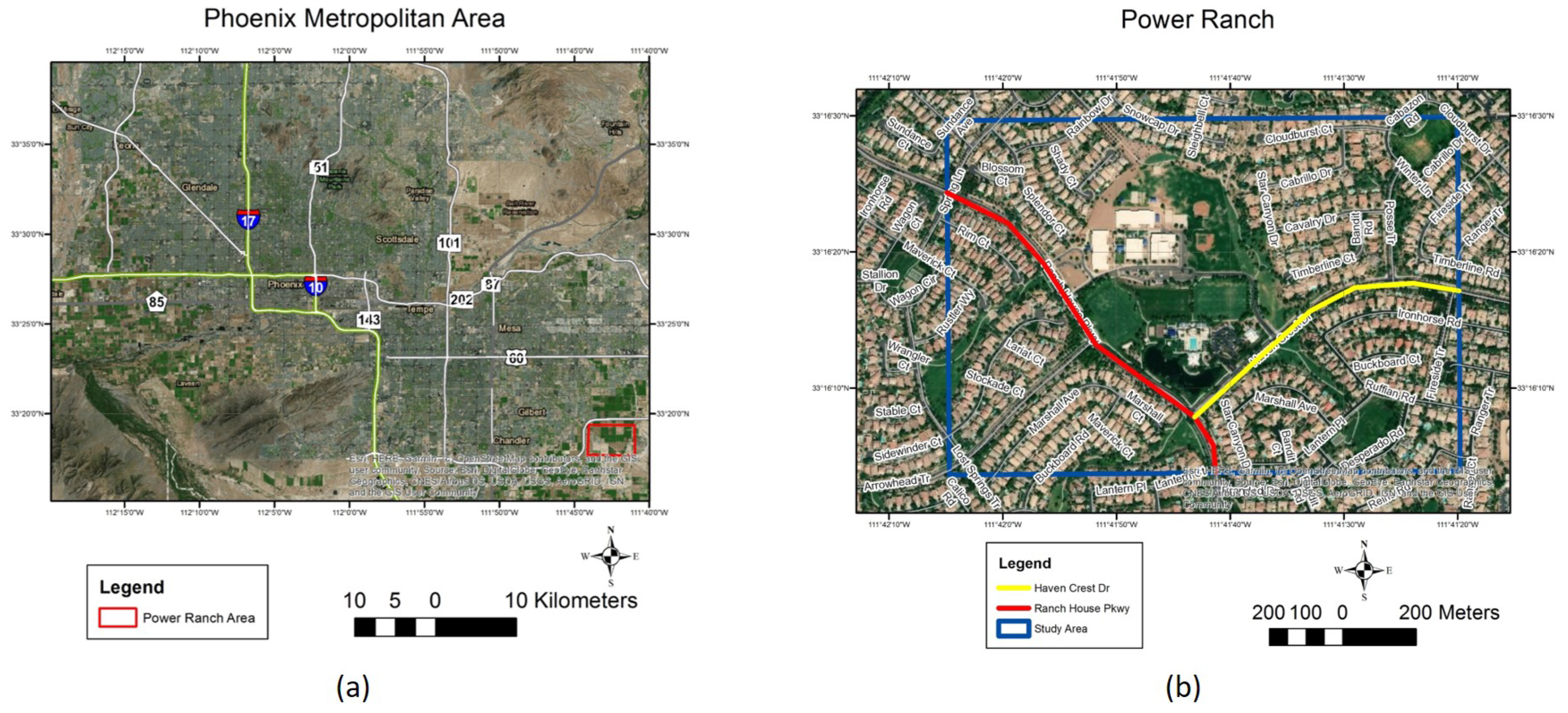
The subject of this study, Power Ranch, is a development within this community. Figure 1a shows the position of Power Ranch in the larger Phoenix Metropolitan Area, while Figure 1b shows the community itself. The specific area of study is also shown within a white box.
The area of study was approximately 1 km in size and consisted of single-family residential units, an elementary school, and a community center; it also included a lake. Two collector streets pass through the area: South Ranch House Parkway in the southeastern direction, and East Haven Crest Drive in the northeastern direction. These are shown in Figure 1b in red and yellow, respectively. Several local streets and many driveways are also present in the area. There are several large parks and a large parking lot, approximately in the center of Figure 1b.
3. Data
3.1. Land Cover
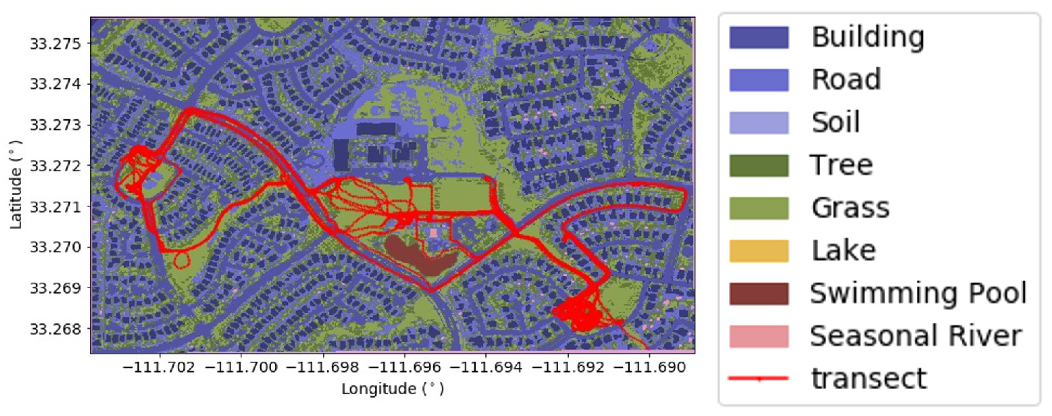
The land-use classification map for the study area was obtained from the work by Li et al. [71] and shown in Figure 2. This data was obtained through aerial imagery followed by digital image processing. A summary of the area covered by different types of land-use is shown in Table 1. About 19% of the area was classified as roads (almost entirely aged asphalt), with nearly the same amount classified as soil, trees, and grass. The soil was mostly artificial granite and mulch, while the grass and trees were artificially irrigated. About 15% of the area was classified as buildings, most of which had concrete tile roofs and stucco walls. The lake was misclassified as a swimming pool, while a small part of the area was misclassified as a lake or a seasonal river, instead of being correctly classified as soil or grass, as evidenced by satellite imagery obtained from Google Earth. These misclassifications were minor in nature, given that both lakes and swimming pools are bodies of water, while the other misclassifications covered only a very small fraction of the total study area. These misclassifications are not expected to have any considerable effect on the rest of the study.
Impervious surfaces (roads and buildings) made up about 35% of the total area, while vegetated surfaces made up the remaining 65%. However, this distribution was uneven, as a large area (about 0.2 km) of the vegetated surfaces were concentrated in the park in the center of the study area, which was surrounded by a dense suburban development composed almost entirely of impervious surfaces, which is typical of suburban areas. These impervious surfaces were in clusters of about 0.1 km in area, consisting of individual houses separated by streets of a much smaller area (of the order of 0.01 km). Smaller vegetated areas (parks) were further distributed within the developments, while the lake covered a much smaller area (about 0.01 km). This heterogeneous land cover configuration is expected to have varying impacts on the microclimate of the area.
Furthermore, these vegetated surfaces were not native to the desert landscape, and were reliant on artificial irrigation. Thus, depending on the availability of water, areas classified as having grass or trees could become soil-covered areas for a period of time.
3.2. Meteorological Data Collection
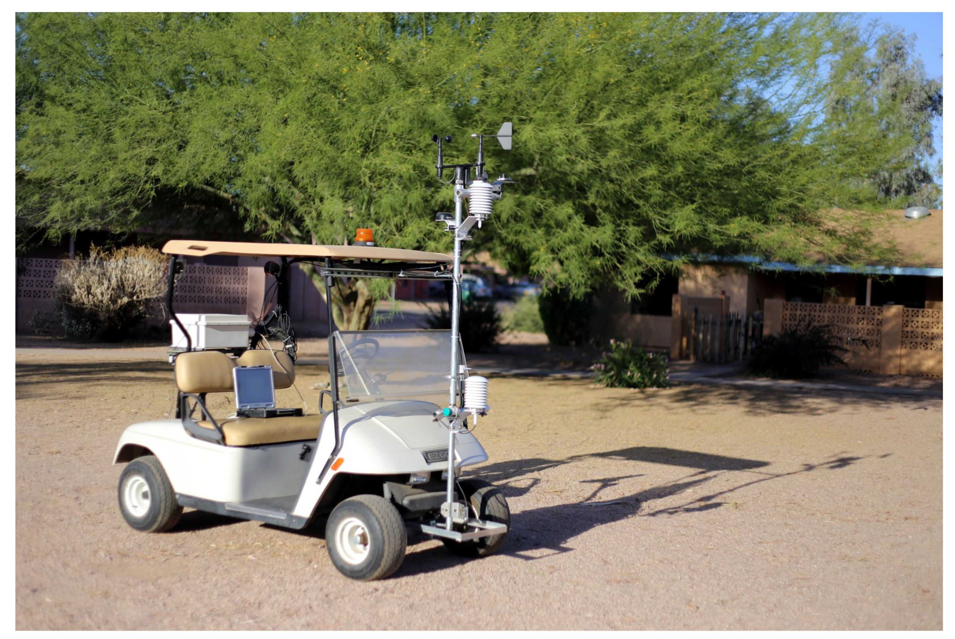
The meteorological data used in this study were taken from a previous study conducted by Häb et al. [72]. The data collected included wind speed, air temperature, surface temperature, and radiant energy. Data collection was performed throughout the day, on 18 June and 30 October 2015, 8 May and 15 September 2014, and 2 February and 13 August 2015, by attaching the instruments onto a mobile platform and driving it around the area along a pre-determined transect. Meteorological variables were recorded once every second. A related study [73] which used the same data showed that local land-use variation led to the development of several microclimatic environments within the urban area. A picture of the mobile platform is shown in Figure 3. Data from 13 August 2015 between 5:00 p.m. and 6:00 p.m. was extracted for this study, as explained below.
Mobile transects are useful for data collection, as they can cover a large area and several different land cover types using a single instrument, although only in areas which are possible to drive through. The disadvantage of using them is that they have limited temporal coverage for any given location, as the platform is continuously moving. In addition, the data has to be corrected for sensor lag and the speed of the platform. For an area of heterogeneous land cover, such as Power Ranch, the data from the transects provides representative meteorological data for the major land cover types, which can be used to validate a predictive numerical model. This validated model can, then, be used to study the microclimate of the entire area and not just along the transect.
For this study, data collected on 13 August 2015 between 5:00 p.m. and 6:00 p.m. was used to model the urban microclimate of the area, as it had the highest average air temperature of all the measured values, with the average 2 m air temperature of 42.91 C. Due to limitations in the computational power available, this study was restricted to modeling the microclimate only for this one hour period; further studies over longer periods (i.e., at a day or seasonal scale) are still necessary for more general results. The transect followed by the platform while collecting data on that day is shown in Figure 2. Most of the measurements over roads were made on the two major collector streets, South Ranch House Parkway and East Haven Crest Drive, while other measurements were made over grass in parks.
Additionally, two pyranometers were also installed on the platform, one pointed upwards at the incoming sunlight and one downwards. By taking the ratio of these two measurements for the points on the transect which were over the roads, the albedo of the roads was found to be about 0.20–0.25, which corresponds to aged asphalt pavements [74,75] (the typical albedo of aged asphalt pavements reported in the literature is 0.10–0.25 [56,76,77]). It was verified from satellite images, as well as visually during data collection, that these were indeed aged asphalt pavements.
4. Model Development
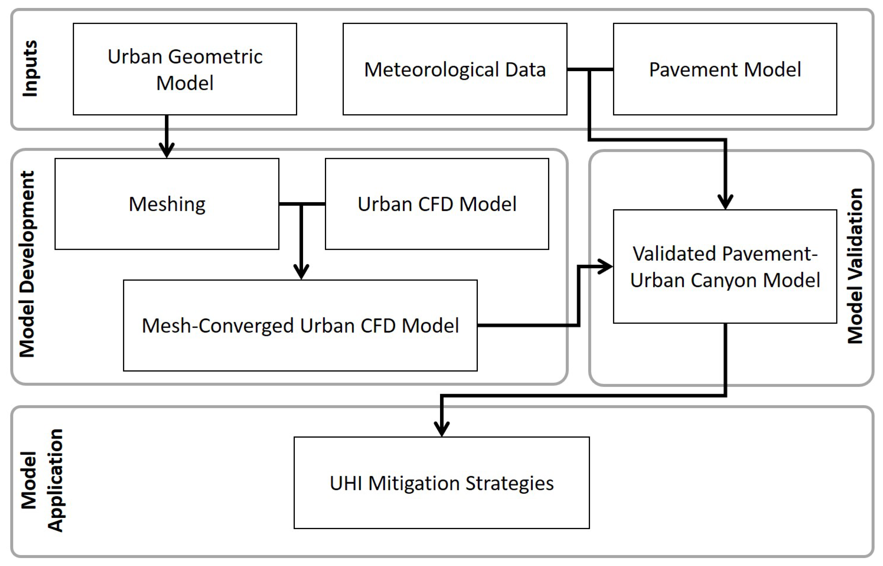
In order to create a validated model of the effect of pavements on the urban microclimate, an uncoupled pavement-urban canyon model was adapted from a previous study [78] and validated for the current one. This validated model was then used to study the effect of cool pavements. The steps used to develop, validate, and then use the model are summarized in Figure 4. The modeling effort consisted of two sub-models: A pavement model, which used a one-dimensional numerical method to calculate the surface temperature of pavements in the urban area; and a three-dimensional Computational Fluid Dynamics (CFD)-based urban canyon model to calculate the air temperature. The variable of interest was the 2 m air temperature, which corresponds to the Canopy Layer UHI. This is important, as most outdoor human activity takes place at this height and, so, it has the most significant impact on urban areas.
As a first step towards validation of the existing model framework with the Power Ranch neighborhood location and features, the model results were compared with the measured 2 m air temperature, surface temperature, and wind speed data collected over the roads. The following subsections describe the model and its validation. The model was evaluated for data collected between 5:00 and 6:00 p.m. on 13 August 2015. The relative humidity (RH) was not included in the model, as the average RH measured at 2 m during the study period was very low (about 10–20%), which would have only a minor impact on the 2 m air temperature. Although RH is an important variable for human comfort, this study was restricted to 2 m air temperature and, thus, RH was outside its scope.
4.1. Pavement Model
The pavement model used was a one-dimensional finite volume heat transfer model, called ILLI-THERM, which accounts for absorbed solar radiation at the surface (which, in turn, depends on the albedo, the geographical location of the study area, and the time), loss of energy through convection and radiation, and the movement of thermal energy through various pavement layers. Details of the model can be found in [47].
Information about the pavement thickness and properties were not available, but the transect measurements showed that the average road surface temperature during the hour of study was 50.35 C. The properties shown in Table 2 were assumed, as those of typical aged asphalt pavements used for local streets, as measured in a previous study [75], together with a far-field wind speed of 0.45 m/s and air temperature of 42.22 C, which were obtained from the nearby (about 10 km away) Phoenix-Mesa Gateway Airport weather station on the hour of analysis.
Using these properties, the calculated surface temperature of the road was 50.22 C, which is very similar to the average measured value. Thus, these properties were used for the pavement model.
4.2. Urban Canyon Model
The urban canyon model used was a three-dimensional CFD model that numerically solves the Reynold’s Average Navier Stokes (RANS) equations, implemented on the open-source CFD solver OpenFOAM [79]. The model consists of the RANS continuity equation shown in Equation (1), the RANS momentum equation shown in Equation (2), and the RANS energy equation shown in Equation (3), where is the RANS velocity component along the direction (), P is the kinematic pressure, is the kinematic viscosity (assumed to be m/s for air), is the turbulent viscosity, is the coefficient of thermal expansion of air (assumed to be /K for air), T is the RANS temperature, is a reference temperature, is the component of the acceleration due to gravity, is the laminar thermal diffusivity of air, and is the turbulent thermal diffusivity.
In order to determine and , a realizable turbulence closure model was used [80] together with standard wall functions [81]. The RANS equations were discretized using second-order schemes.
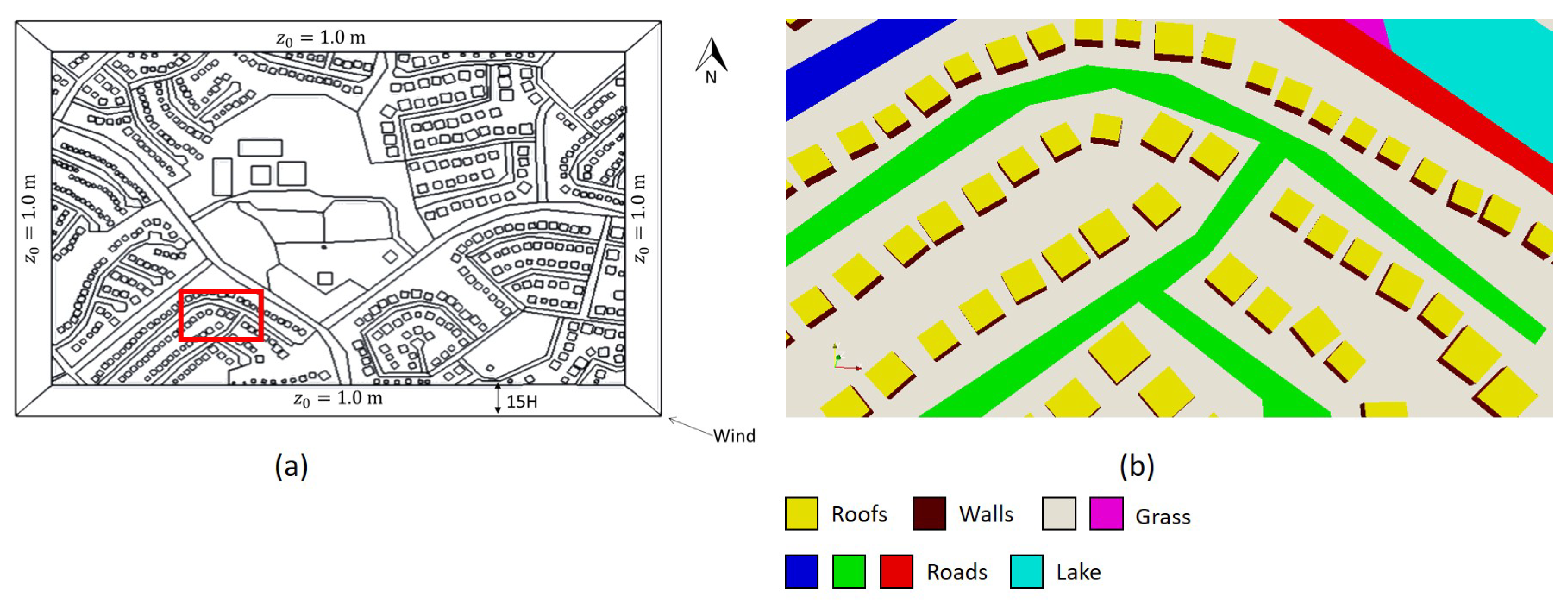
As a first step, the Power Ranch area was converted into an at-scale digital geometric model, as shown in Figure 5a, with a close-up image of the buildings, road, and natural vegetation in Figure 5b. As most of the buildings in the area were single-family homes, the height of all buildings was assumed to be m. Following best-practice guidelines for urban CFD [82], an additional boundary of width 15 H (75 m), perpendicular to the outer limits of the study area, was added. In the outer extent boundary, buildings were not explicitly modeled, but a aerodynamic roughness length m was added, representing more suburban land-use with regularly-spaced buildings [83], which corresponds to the land cover around the study area, as can be seen in Figure 1b. The aerodynamic roughness length is the height at which the mean wind speed becomes zero, and is used to model land cover without explicitly resolving features such as buildings and trees. The top of the model was extended to a height of 15 H (75 m) above the top of the buildings. Small-scale objects, primarily trees and shrubs, were not directly modeled and, instead, the natural surfaces were modeled with a aerodynamic roughness length of 0.10 m, representing a roughly open terrain with a few trees and low hedges. Similarly, features on buildings (like windows or doors) and curb-side features in the residential areas were also not modeled. This was done to reduce the computational requirements to solve the equations.
For boundary conditions, meteorological data from the nearby Phoenix-Mesa Gateway Airport (measured at 1.5 m), together with surface temperature measurements from the mobile platform, were used, as shown in Table 3. The far-field wind speed at the time of analysis was 0.45 m/s (about 1 mph) at a height of 1.5 m from an East-Southeast (ESE) direction. Using this value, an Atmospheric Boundary Layer (ABL) wind profile was applied at the boundaries, using the same aerodynamic roughness length m, based on the recommendations of Raupack et al. [84].
The far-field air temperature, as measured at the airport, was 42.22 C, and this was modeled as a uniform profile at the boundaries. The surface temperature of natural and artificial surfaces was based on the average values measured by the mobile platform: 50.36 C for roads, 48.19 C for natural surfaces, and 48.62 C for walls. As the platform could not measure roof temperatures, it was assumed that the roof was at the same temperature as the walls. This is most likely an underestimation of the roof temperature, as Stefanov et al. [85] showed that roof temperatures in this area could rise to well over 70 C. However, in the absence of measured values corresponding to the hour at which this study was performed, this assumption was used. Furthermore, as the platform could not measure surface temperatures over water, it was assumed that the lake had the same surface temperature as the far-field air temperature. This was, again, possibly an overestimation, as the water would be significantly cooler than the air, but was used in the absence of measured data. It is possible that the effects of these over- and under-estimations would cancel each other out, to some extent, which will be verified during model validation.
4.3. Grid Convergence
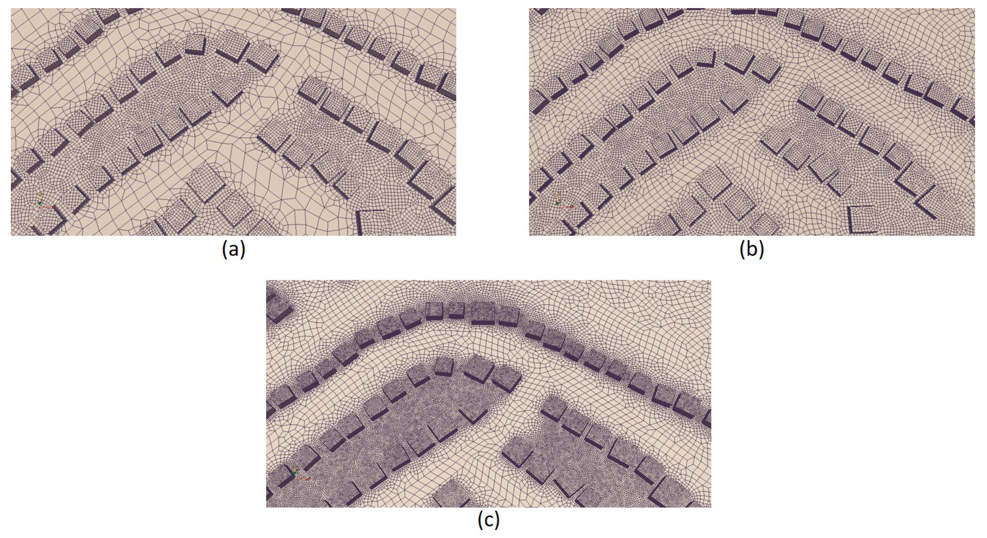
The digital model of the study area shown in Figure 5 was discretized using the mesh extrusion method developed by van Hooff and Blocken [86]. The 2D plan of the model (excluding buildings) was first discretized into quadrilateral elements of sizes varying from 1–5 m, and then the 2D mesh was extruded up to the height of the buildings. Next, the roof surfaces were discretized and the entire model was further extruded up to the top of the model. In this way, a high-quality hexahedral mesh could be generated. As a final step, boundary layer elements were added near walls, which were much smaller than 1 m. The meshing was done using the open-source meshing engine, Gmsh [87]. All meshes generated consisted of over 99.9% hexahedral elements, less than 0.1% prismatic elements, and no tetrahedral elements.
A grid convergence study was performed to ensure that the results from the model did not depend on the size of the mesh. Three mesh cases were developed by approximately halving the size of cells from the preceding case. These are shown in Table 4, with images from one part of the study area shown in Figure 6.
For each of these mesh cases, the model was run until scaled residuals fell below ; except for pressure, where the final residuals were below . Lift and drag coefficients on the walls (which were functions of the wind velocity fields) were also monitored and, at convergence, they changed by less than 0.1% between iterations. The variables of interest in this study were the average wind speed and air temperature at a 2 m height over the two collector roads, given that most of the data was collected over the streets. These two variables were extracted from the model output.
To test for grid convergence, the difference between the average wind speed and air temperature over the roads at a 2 m height between the meshes was evaluated. For the Medium mesh, the difference was evaluated against the results obtained from the Coarse mesh, while, for the Fine mesh, the result from the Medium mesh was used. In addition to the difference, the Grid Convergence Index (GCI) recommended by Roache [88] was also calculated using Equation (4), where is the difference between the average wind speed or air temperature at 2 m height, is the refinement ratio for an unstructured mesh (the ratio between the number of cells in the fine grid to the coarse grid raised to the inverse of the number of dimensions), and p is the order of convergence of the numerical scheme (second-order in this case, ). The GCI scales the difference between the variables of interest to account for grid refinement and order of convergence, providing a uniform way of reporting grid convergence studies. Both the differences and GCI for the mesh cases are shown in Table 5.
For both the Medium and Fine meshes, the differences were small, with a maximum difference of 1.33% between the average wind speed over the roads. Similarly, the GCI values were also small, with the highest value being 7.77% between Medium and Coarse. Considering the inherent uncertainty in turbulence modeling and the unstructured nature of the mesh, these differences are acceptable. Thus, both the Medium and the Fine mesh cases were convergent within acceptable tolerance. However, as the Medium case was computationally faster, it was adopted for the remainder of the study.
4.4. Validation
Wind speed and air temperature over the road obtained from the Medium mesh case, as described above, were compared to the values measured during the hour of analysis by the mobile platform. As the platform moved along the transect, the points along which the measurements were taken changed continuously. Data obtained from between 5:00 p.m. and 6:00 p.m. was extracted and cleaned, yielding about 1000 points each for 2 m air temperature and wind speed. Points along the transect may not coincide with the center of a 3D element and, therefore, a point-to-point comparison of the two was not possible. This was in contrast to studies that used fixed weather stations for model validation. In this study, data from the computational model over the two main collector streets was extracted, yielding about 2000 points of data for each of the cases. The statistics of these two sets of data (measured and model) were, then, compared for validation. This approach is also logically valid, as the effects of the UHI (e.g., thermal comfort or energy use) depends on the value of air temperature within a localized region, and not the value at any single point.
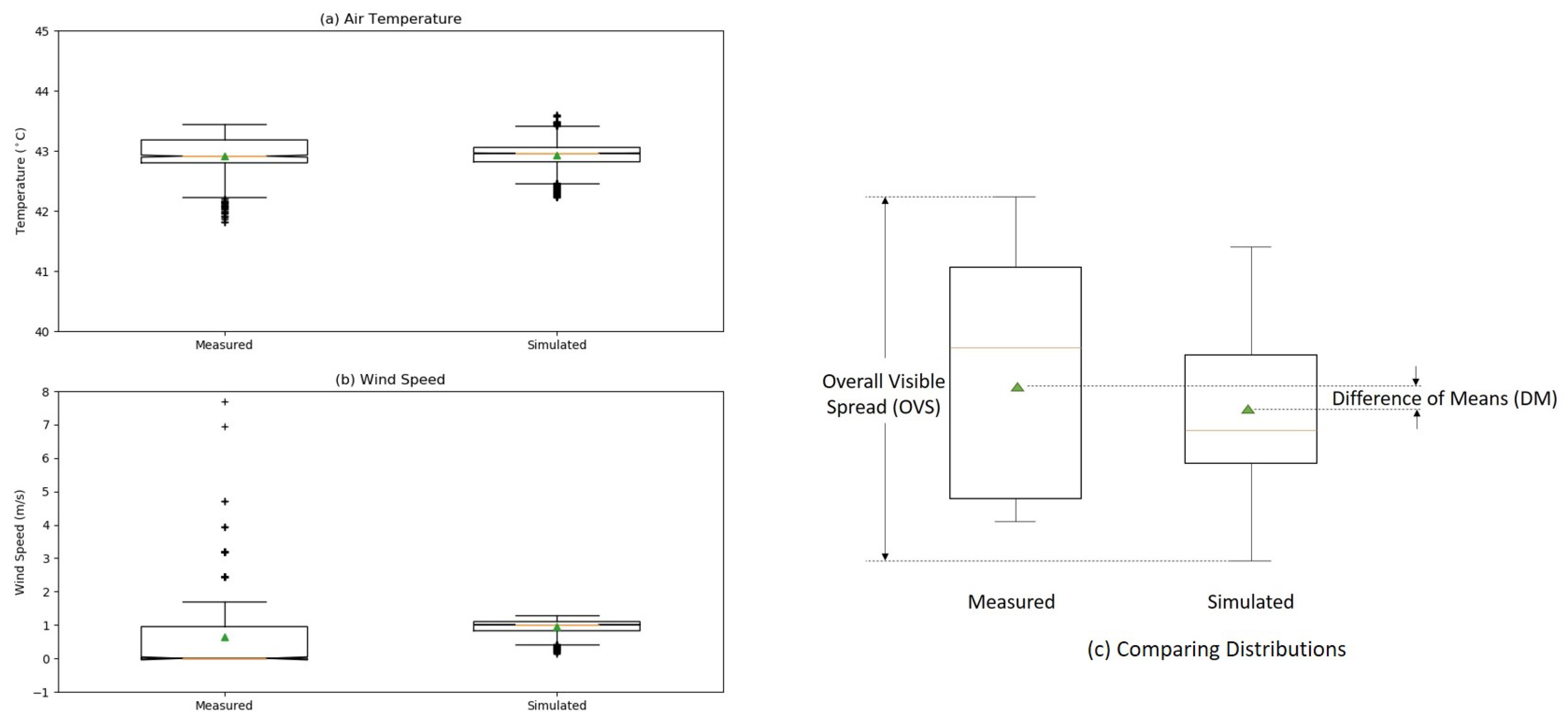
The results of the statistical comparison are shown in Figure 7a,b, in the form of box-plots. It can be seen that the measured values, especially the wind speed, were highly skewed, with a large difference between the mean and the median as well as a number of outliers. Therefore, the validation must take both the mean and the distribution of the variables into account.
Two metrics were used, as shown in Figure 7c. The Difference of Means (DM) is the difference between the mean of the measured and simulated variables. The Overall Visible Spread (OVS) was the overall range of the combined measured and simulated data, which is a measure of its distribution. An effective Coefficient of Variance COV = DM/OVS was defined as a measure of variation between the measured and simulated data for each variable.
The DM for 2 m air temperature was just 0.03 C, while that between wind speeds was 0.47 m/s. The corresponding COV were 3.0% and 28.0%, respectively. From these metrics, it can be concluded that the simulation showed excellent agreement with measured 2 m air temperatures, but only moderate agreement with wind speed. The difference in wind speed can be explained by the presence of a number of small-scale structures in the physical domain—such as trees, shrubs, and other vehicles—which decreased the local wind speed, but which were not explicitly modeled in the computational domain. As the mobile platform drove past these structures, it recorded a wind speed of zero or a low value below 1 m/s and, hence, over 50% of the recorded data was zero, as can be seen in Figure 7b, where the median of the measured data is zero. Whereas, in the computational domain, they were not explicitly modeled and, thus, a higher wind speed was recorded at the corresponding locations, which, in turn, pushed the entire distribution to a higher mean value.
As the primary aim of this study was to examine the 2 m air temperature, the high degree of agreement between the measured and simulated temperatures and moderate agreement between the wind speeds were considered satisfactory for validation. This validated model was used to study UHI mitigation strategies.
5. UHI Mitigation
5.1. Strategies
To demonstrate the effectiveness of cool surfaces to mitigate UHI in the study area, five strategies were explored and compared to the base case. These are shown in Table 6. The Existing Pavements scenario modeled the existing conditions of the area, with aged asphalt pavements. The measured average pavement surface temperature at 5:00 p.m. of 50.36 C was used, in this case. As shown in a previous study [74], typical asphalt pavements achieve their steady-state albedo of 0.20–0.25 in about a year. In order to simulate the microclimate of the area with newly-constructed asphalt pavements, the New Asphalt Pavements scenario was run, in which the diffusivity of the pavements remained the same, but their albedo was reduced to a typical value of 0.05 [74,75].
Next, four cooling strategies were explored. In the Typical Concrete Pavements scenario, all the asphalt roads in the study area were replaced with typical concrete ones by increasing the diffusivity and albedo to the typical concrete values of 2.0 mm/s and 0.35, respectively. This could be achieved using a concrete overlay (white-topping) [89,90]. Next, in the Reflective Concrete Pavements scenario, the albedo of the typical concrete was increased to a value of 0.50, which is a reasonable long-term albedo that can be expected from in-service reflective concrete pavements, such as one made with white cement [91].
In the Reflective Roofs and Walls scenario, the albedo of the roofs and walls was increased to 0.60 by spraying them with a thin layer of a reflective coating, while keeping the pavements unchanged. These coatings are usually water- or solvent-based containing a high-albedo pigment and are typically easy to apply, but with a more limited service life than reflective concrete. Li et al. [92] discussed several types of reflective coatings having an average albedo of about 0.60, which was adopted for this mitigation scenario. For simplicity, the thermal diffusivity was assumed to be the same as that of the existing pavements, although field measurements of roofs and walls would be necessary for a more accurate estimate of the surface temperature. Finally, a comprehensive Reflective Coating scenario was considered, in which all the pavements, roofs, and walls were sprayed with a thin layer of a reflective coating. The thermal diffusivity of the existing asphalt pavements (1.5 mm/s) was, again, used for this scenario, as the thin coatings would not change this significantly.
For all the scenarios, the thermal diffusivity and albedo were used to evaluate the pavement, roof, and wall surface temperatures, which was then used as a boundary condition for the urban canyon model. The calculated surface temperatures are shown in the last column of Table 6. The last column also indicates which surface was modified, with the surface temperature of the other surfaces being kept the same as in the Existing Pavements scenario. For all cases, the surface temperature of the natural surfaces was kept the same as the measured values, as those would not change in any of the mitigation strategies.
5.2. Results and Discussion
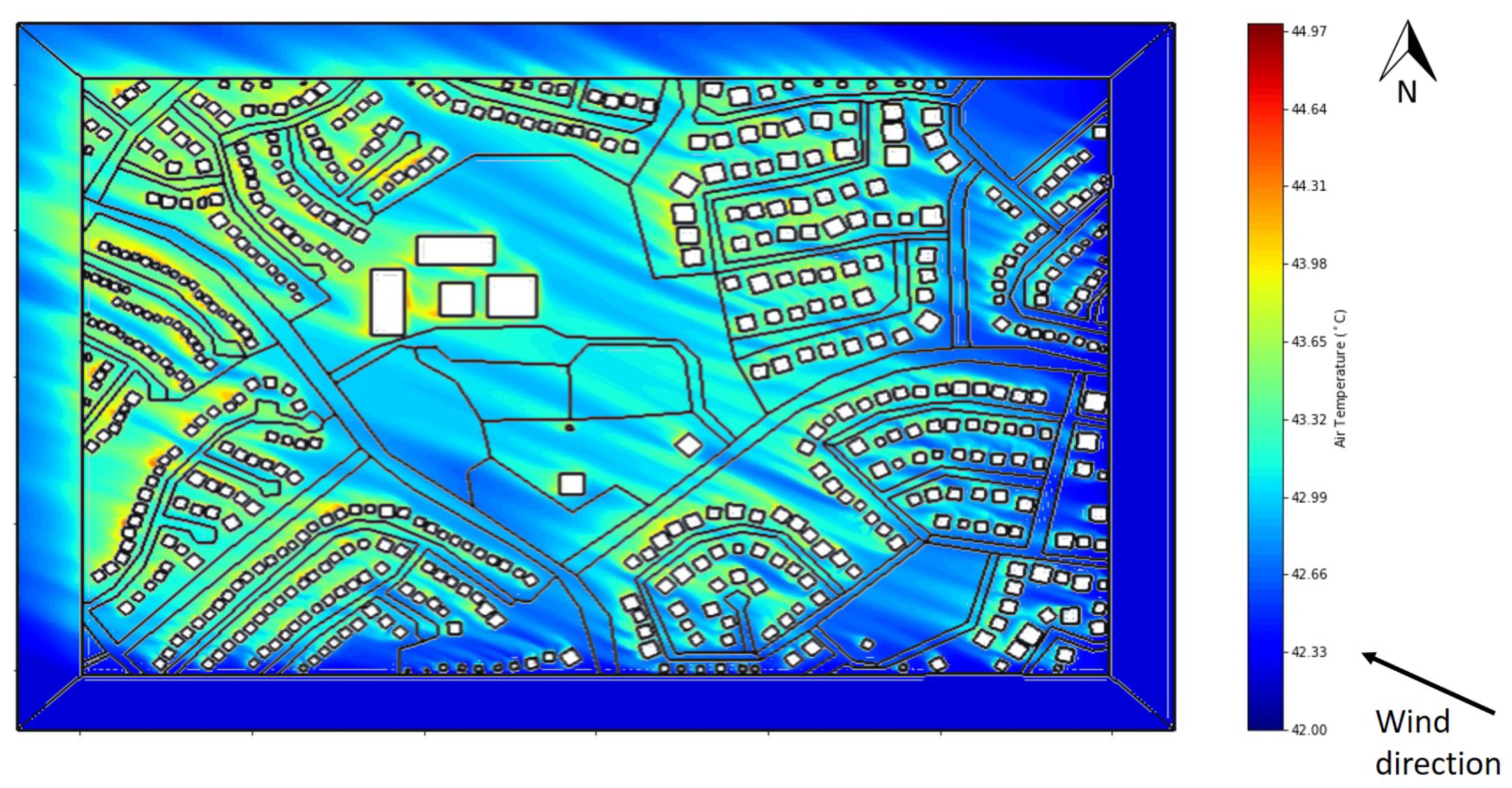
The simulated air temperature at a 2 m height for the Existing Pavements case is shown in Figure 8, with the wind direction (ESE) also marked. The temperature contours can be observed to follow the wind direction. As the air is heated by flowing over warmer surfaces, the residents in the northwestern part of the area experienced a higher air temperature, of over 44 C, representing a microscale UHI intensity of about 2 C. Temperatures were even higher immediately downstream of buildings, due to heating by the walls and roofs.
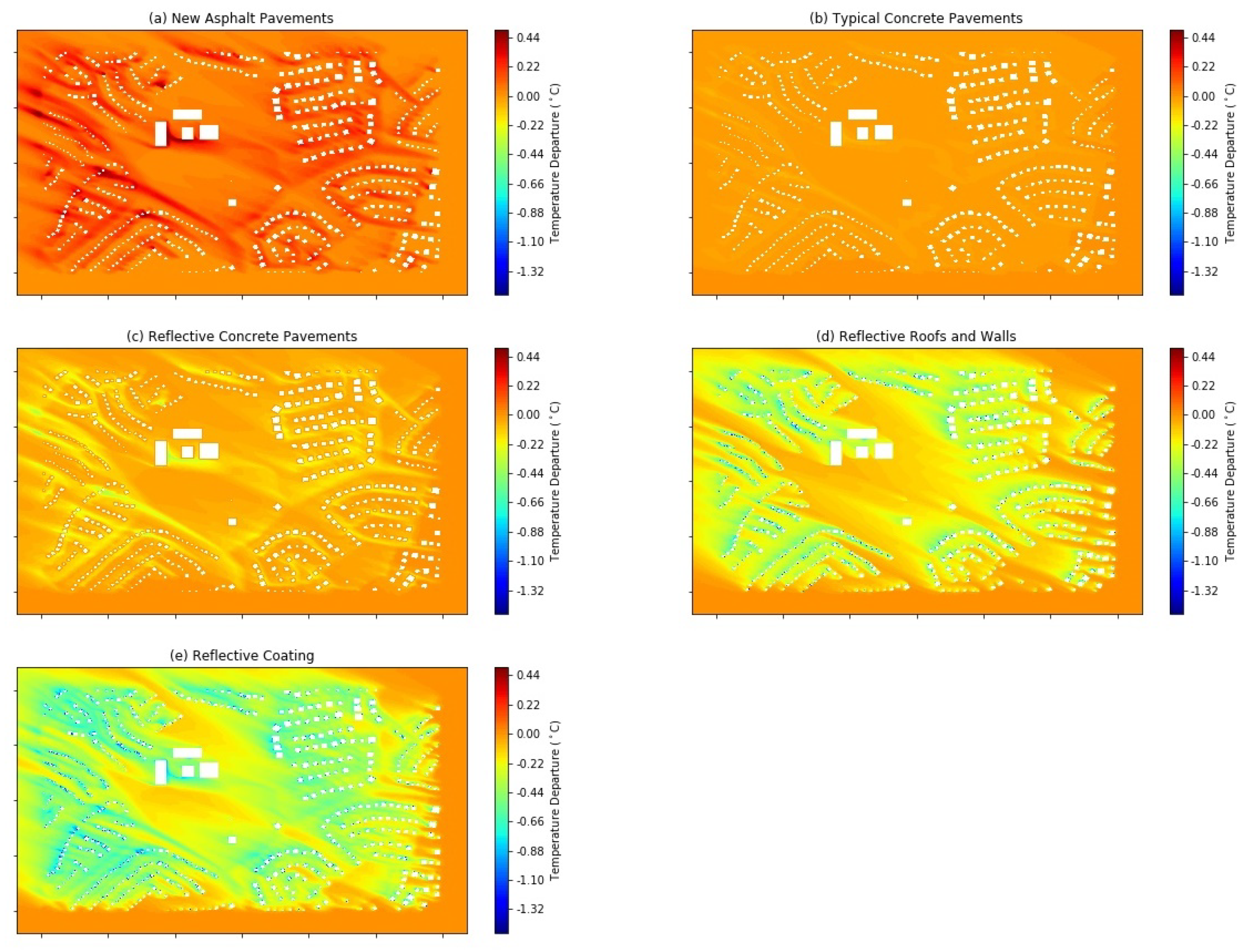
The five UHI mitigation scenarios (New Asphalt Pavements, Typical Concrete Pavements, Reflective Concrete Pavements, Reflective Roofs and Walls, and Reflective Coating) were evaluated and the difference between their 2 m air temperature and that of the Existing Pavements scenario are shown in Figure 9. For the New Asphalt Pavements scenario (shown in Figure 9a), developments downstream of collector roads had an increased 2 m air temperature of up to 0.50 C, with the most widespread increase being seen in the northwestern part of the domain, which consisted of a dense cluster of impervious developments. Furthermore, as the surface temperature of the natural surfaces remained the same, the air temperature over and downstream of these surfaces also remained approximately the same. This was particularly evident for the large central park, which largely had the same 2 m air temperature as the base case, whereas the smaller vegetated areas had a greater increase in air temperature.
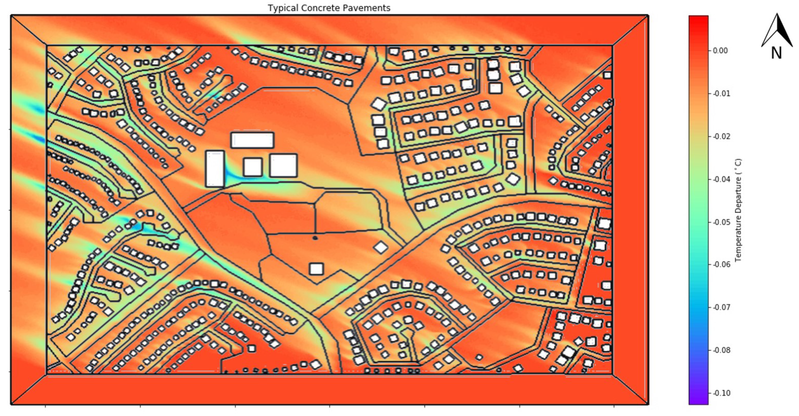
In the Typical Concrete Pavements scenario, there was very little change in air temperature. Figure 10 shows the temperature differences for this scenario on a finer scale. Again, areas downstream of the collector roads had a lower temperature, but the peak departure was only about −0.06 C in the northwestern developments. The vegetated surfaces had virtually no difference at all. Thus, simply resurfacing all the asphalt pavements with typical concrete in this neighborhood did not have any significant effect on the 2 m air temperature during the analysis period. This is possibly due to the relatively small area of the roads, with respect to other impervious and vegetated surfaces.
The Reflective Concrete Pavements scenario showed a greater decrease in air temperature than the Typical Concrete Pavements scenario. The 2 m air temperature downstream of the two collector roads decreased by 0.20–0.40 C, while there was a decrease of about 0.20 C in some parts of the central park, as well. These results can be compared to other studies, as summarized by Santamouris [55], where the reduction in air temperature due to reflective pavements ranged from 0.15–3.0 C. Similarly, [56] summarized a handful of other studies, and also reported a reduction of 0.40–0.60 C in UHI intensity through cool pavements. While these results varied by location, albedo, and extent of the application of pavements, the observed reduction of 0.20–0.40 C in this study fell within these reported values. Thus, replacing all the asphalt pavements in the study area with more reflective concrete pavements decreased the air temperature. However, once again, the large area of the central park had only a limited decrease in 2 m air temperature.
The Reflective Roofs and Walls scenario showed an even higher decrease in 2 m air temperature, as shown in Figure 9d. The peak departure was about 0.40–0.70 C. This higher decrease was due to the large number of buildings, which were dispersed in almost every part of the study area, as compared to roads, which were less evenly distributed. Santamouris [93] reviewed several studies on the effectiveness of reflective roofs and found that, for an increase in albedo of only roofs by 0.1 globally, an average reduction of 0.10–0.33 C can be expected. A higher decrease than this was achieved in this scenario, because both roofs and walls were made reflective. However, over the central park, only a small departure, between 0.0 and 0.1 C, could be achieved. Thus, making roofs and walls reflective was more effective than making the pavements reflective for this study area and for the meteorological conditions simulated.
The final scenario considered was Reflective Coating, which was a comprehensive approach that increased the albedo of all artificial surfaces. In this case, a higher temperature reduction was achieved downstream of roads, buildings, and roofs. In the northwestern developments, the air temperature reduction was between 0.80–1.00 C as compared to existing temperatures, which was comparable to the reduction in UHI intensity predicted by [49] through the adoption of cool surfaces in a different climatic location (the eastern US), as well as by [51] through global adoption of cool surfaces. The air temperature also decreased over the central park by about 0.10–0.20 C, indicating the strong downstream effect of the cool surfaces. Thus, a comprehensive strategy to increase the albedo of pavements, roofs, and walls should lead to decreased air temperatures throughout the study area, with a large UHI reduction in developments downstream of the impervious surfaces.
For urban planners, these results have different implications for new and existing suburban developments. In new developments, planners and developers should be encouraged to make pavements, roofs, and walls reflective, so as to maximize UHI mitigation. However, for existing developments, it may be more difficult to achieve the goal of reduced UHI. Encouraging homeowners to coat their roofs and walls with a reflective coating would be effective, but would pose practical difficulties due to the large number of stakeholders (homeowners) involved. Instead, city engineers may be encouraged to make the roads reflective, using either reflective overlays or coatings. While this would be less effective than modifying roofs and walls, it would be easier to achieve and more rapidly implemented.
6. Conclusions
The Urban Heat Island (UHI) effect is a commonly-observed phenomenon caused by increasing urban sprawl. UHI manifests in the form of increased urban air temperatures, and influences water use, air quality, public health, and so on. Cool surfaces, including pavements, roofs, and walls, have been suggested to mitigate UHI. However, the UHI is a heterogeneous effect, with local land-use patterns, construction materials, building forms, and climatic factors affecting possible mitigation strategies.
The microclimate of Power Ranch, a suburban development in the Phoenix Metropolitan Area, was studied for conditions at 5:00 p.m. on 13 August 2015, when the far-field air temperature was measured at over 42 C with a low wind speed of 0.45 m/ at a 1.5 m height from an ESE direction. An uncoupled pavement-urban canyon CFD model was developed and validated for the Power Ranch area. The area had two collector streets and several local streets, all of which consisted of aged asphalt pavements. Artificial surfaces (pavements, roofs, and walls) covered about 35% of the area, with the remaining 65% being covered by natural surfaces (grass, trees, soil, and water bodies).
The effects of changing the pavement surfaces was investigated through five scenarios. In the first scenario, all aged asphalt surfaces were replaced with new asphalt surfaces. This led to an overall increase in air temperature at a 2 m height, with the maximum increase of 0.50 C being observed in the northwestern parts of the area; which were downstream of the collector roads. In the second scenario, the existing aged asphalt pavements were replaced with typical concrete pavements. This strategy, for this neighborhood, led only to a slightly decreased air temperature of less than 0.1 C, with the large area of the natural surfaces largely negating the decrease in temperature from the cooler pavements.
The third scenario replaced all pavement surfaces with more reflective concrete pavements. This led to a decrease in air temperature by about 0.20–0.40 C downstream of the collector roads. However, there was no significant reduction over most of the natural surfaces. A fourth scenario coated all roofs and walls with a reflective coating, leading to a higher 2 m air temperature reduction, of about 0.40–0.70 C, and a small decrease, of 0.00–0.10 C, over the natural surfaces. Finally, a fifth scenario increased the albedo of all artificial surfaces with the same reflective coating. This scenario resulted in the largest decrease in air temperature, by about 0.80–1.00 C, in the northwestern development downstream of the collector roads, as well as a decrease of 0.10–0.20 C over the natural surfaces.
Thus, for the meteorological conditions evaluated for the Power Ranch suburban community, changing all walls, roofs, and pavements into reflective surfaces was the most effective strategy for mitigating UHI. Using only reflective walls and roofs had a greater mitigating impact than using only reflective pavements. For existing suburban developments, applying reflective pavements is likely to be implemented faster, whereas reflective roofs and walls would require the participation of a large number of homeowners. These conclusions are only for the particular land cover type, analysis period, and meteorological conditions of this study. A similar type of study would need to be conducted for the unique conditions of other locations for the mitigation of UHI.
Author Contributions
Conceptualization, S.S. and J.R.; Data curation, B.R. and A.M.; Formal analysis, S.S.; Funding acquisition, J.R., B.R., and A.M.; Investigation, S.S.; Methodology, S.S.; Supervision, J.R. and A.M.; Validation, S.S.; Visualization, S.S.; Writing—original draft, S.S.; Writing—review & editing, S.S., J.R., B.R., and A.M.
Funding
The data collection and land cover classification parts of this work work were supported by the National Science Foundation (NSF) under EaSM Grant EF-1049251 and via a grant from the Salt River Project awarded to Arizona State University. The opinions expressed are those of the authors, and not necessarily the funding agencies. Funding for the computational parts of this study was provided by the US Department of Transportation (USDOT) through the University Transportation Center for Highway Pavement Preservation (UTCHPP) at Michigan State University with Contract Number DTR13-G-UTC44.
Acknowledgments
The authors thank the Power Ranch Community Association for their cooperation with the data collection efforts.
Conflicts of Interest
The authors declare no conflict of interest.
References
- Hasse, J.E.; Lathrop, R.G. Land resource impact indicators of urban sprawl. Appl. Geogr. 2003, 23, 159–175. [Google Scholar] [CrossRef]
- Ewing, R.H. Characteristics, causes, and effects of sprawl: A literature review. In Urban Ecology; Springer: Berlin, Germany, 2008; pp. 519–535. [Google Scholar]
- Huang, J.; Lu, X.X.; Sellers, J.M. A global comparative analysis of urban form: Applying spatial metrics and remote sensing. Landsc. Urban Plan. 2007, 82, 184–197. [Google Scholar] [CrossRef]
- Mieszkowski, P.; Mills, E.S. The causes of metropolitan suburbanization. J. Econ. Perspect. 1993, 7, 135–147. [Google Scholar] [CrossRef]
- Edmonston, B. Metropolitan population deconcentration in Canada, 1941–1976. Can. Stud. Popul. 1983, 10, 49–70. [Google Scholar] [CrossRef]
- Ewing, R.; Schmid, T.; Killingsworth, R.; Zlot, A.; Raudenbush, S. Relationship between urban sprawl and physical activity, obesity, and morbidity. In Urban Ecology; Springer: Berlin, Germany, 2008; pp. 567–582. [Google Scholar]
- Sturm, R.; Cohen, D.A. Suburban sprawl and physical and mental health. Public Health 2004, 118, 488–496. [Google Scholar] [CrossRef] [PubMed]
- Ditchkoff, S.S.; Saalfeld, S.T.; Gibson, C.J. Animal behavior in urban ecosystems: Modifications due to human-induced stress. Urban Ecosyst. 2006, 9, 5–12. [Google Scholar] [CrossRef]
- Miller, M.D. The impacts of Atlanta’s urban sprawl on forest cover and fragmentation. Appl. Geogr. 2012, 34, 171–179. [Google Scholar] [CrossRef]
- Stone, B., Jr. Urban sprawl and air quality in large US cities. J. Environ. Manag. 2008, 86, 688–698. [Google Scholar] [CrossRef] [PubMed]
- Haase, D.; Nuissl, H. Does urban sprawl drive changes in the water balance and policy?: The case of Leipzig (Germany) 1870–2003. Landsc. Urban Plan. 2007, 80, 1–13. [Google Scholar] [CrossRef]
- Morote, Á.F.; Hernández, M. Urban sprawl and its effects on water demand: A case study of Alicante, Spain. Land Use Policy 2016, 50, 352–362. [Google Scholar] [CrossRef] [Green Version]
- Santamouris, M.; Cartalis, C.; Synnefa, A.; Kolokotsa, D. On the impact of urban heat island and global warming on the power demand and electricity consumption of buildings—A review. Energy Build. 2015, 98, 119–124. [Google Scholar] [CrossRef]
- Parsaee, M.; Joybari, M.M.; Mirzaei, P.A.; Haghighat, F. Urban heat island, urban climate maps and urban development policies and action plans. Environ. Technol. Innov. 2019, 14, 100341. [Google Scholar] [CrossRef]
- Rasul, A.; Balzter, H.; Smith, C.; Remedios, J.; Adamu, B.; Sobrino, J.; Srivanit, M.; Weng, Q. A review on remote sensing of urban heat and cool islands. Land 2017, 6, 38. [Google Scholar] [CrossRef]
- Tran, H.; Uchihama, D.; Ochi, S.; Yasuoka, Y. Assessment with satellite data of the urban heat island effects in Asian mega cities. Int. J. Appl. Earth Obs. Geoinf. 2006, 8, 34–48. [Google Scholar] [CrossRef]
- Estoque, R.C.; Murayama, Y.; Myint, S.W. Effects of landscape composition and pattern on land surface temperature: An urban heat island study in the megacities of Southeast Asia. Sci. Total. Environ. 2017, 577, 349–359. [Google Scholar] [CrossRef]
- Kotharkar, R.; Ramesh, A.; Bagade, A. Urban heat island studies in South Asia: A critical review. Urban Clim. 2018, 24, 1011–1026. [Google Scholar] [CrossRef]
- Deilami, K.; Kamruzzaman, M.; Liu, Y. Urban heat island effect: A systematic review of spatio-temporal factors, data, methods, and mitigation measures. Int. J. Appl. Earth Obs. Geoinf. 2018, 67, 30–42. [Google Scholar] [CrossRef]
- Arnfield, A.J. Two decades of urban climate research: A review of turbulence, exchanges of energy and water, and the urban heat island. Int. J. Climatol. 2003, 23, 1–26. [Google Scholar] [CrossRef]
- Chapman, S.; Watson, J.E.; Salazar, A.; Thatcher, M.; McAlpine, C.A. The impact of urbanization and climate change on urban temperatures: A systematic review. Landsc. Ecol. 2017, 32, 1921–1935. [Google Scholar] [CrossRef]
- Hafner, J.; Kidder, S.Q. Urban heat island modeling in conjunction with satellite-derived surface/soil parameters. J. Appl. Meteorol. 1999, 38, 448–465. [Google Scholar] [CrossRef]
- Memon, R.A.; Leung, D.Y.; Liu, C.H. An investigation of urban heat island intensity (UHII) as an indicator of urban heating. Atmos. Res. 2009, 94, 491–500. [Google Scholar] [CrossRef]
- Gaffin, S.; Rosenzweig, C.; Khanbilvardi, R.; Parshall, L.; Mahani, S.; Glickman, H.; Goldberg, R.; Blake, R.; Slosberg, R.; Hillel, D. Variations in New York city’s urban heat island strength over time and space. Theor. Appl. Climatol. 2008, 94, 1–11. [Google Scholar] [CrossRef]
- Chow, W.T.; Roth, M. Temporal dynamics of the urban heat island of Singapore. Int. J. Climatol. 2006, 26, 2243–2260. [Google Scholar] [CrossRef]
- Buyantuyev, A.; Wu, J. Urban heat islands and landscape heterogeneity: Linking spatiotemporal variations in surface temperatures to land-cover and socioeconomic patterns. Landsc. Ecol. 2010, 25, 17–33. [Google Scholar] [CrossRef]
- Debbage, N.; Shepherd, J.M. The urban heat island effect and city contiguity. Comput. Environ. Urban Syst. 2015, 54, 181–194. [Google Scholar] [CrossRef]
- Stone, B.; Hess, J.J.; Frumkin, H. Urban form and extreme heat events: are sprawling cities more vulnerable to climate change than compact cities? Environ. Health Perspect. 2010, 118, 1425–1428. [Google Scholar] [CrossRef]
- Zhang, H.; Qi, Z.F.; Ye, X.Y.; Cai, Y.B.; Ma, W.C.; Chen, M.N. Analysis of land use/land cover change, population shift, and their effects on spatiotemporal patterns of urban heat islands in metropolitan Shanghai, China. Appl. Geogr. 2013, 44, 121–133. [Google Scholar] [CrossRef]
- Ward, K.; Lauf, S.; Kleinschmit, B.; Endlicher, W. Heat waves and urban heat islands in Europe: A review of relevant drivers. Sci. Total Environ. 2016, 569, 527–539. [Google Scholar] [CrossRef]
- Van Hove, L.; Jacobs, C.; Heusinkveld, B.; Elbers, J.; Van Driel, B.; Holtslag, A. Temporal and spatial variability of urban heat island and thermal comfort within the Rotterdam agglomeration. Build. Environ. 2015, 83, 91–103. [Google Scholar] [CrossRef] [Green Version]
- Connors, J.P.; Galletti, C.S.; Chow, W.T. Landscape configuration and urban heat island effects: Assessing the relationship between landscape characteristics and land surface temperature in Phoenix, Arizona. Landsc. Ecol. 2013, 28, 271–283. [Google Scholar] [CrossRef]
- Zhou, W.; Huang, G.; Cadenasso, M.L. Does spatial configuration matter? Understanding the effects of land cover pattern on land surface temperature in urban landscapes. Landsc. Urban Plan. 2011, 102, 54–63. [Google Scholar] [CrossRef]
- Zhibin, R.; Haifeng, Z.; Xingyuan, H.; Dan, Z.; Xingyang, Y. Estimation of the relationship between urban vegetation configuration and land surface temperature with remote sensing. J. Indian Soc. Remote Sens. 2015, 43, 89–100. [Google Scholar] [CrossRef]
- Zheng, B.; Myint, S.W.; Fan, C. Spatial configuration of anthropogenic land cover impacts on urban warming. Landsc. Urban Plan. 2014, 130, 104–111. [Google Scholar] [CrossRef]
- Jenerette, G.D.; Harlan, S.L.; Buyantuev, A.; Stefanov, W.L.; Declet-Barreto, J.; Ruddell, B.L.; Myint, S.W.; Kaplan, S.; Li, X. Micro-scale urban surface temperatures are related to land-cover features and residential heat related health impacts in Phoenix, AZ USA. Landsc. Ecol. 2016, 31, 745–760. [Google Scholar] [CrossRef]
- Li, X.; Li, W.; Middel, A.; Harlan, S.; Brazel, A.; Turner Ii, B. Remote sensing of the surface urban heat island and land architecture in Phoenix, Arizona: Combined effects of land composition and configuration and cadastral–demographic–economic factors. Remote Sens. Environ. 2016, 174, 233–243. [Google Scholar] [CrossRef]
- Du, H.; Ai, J.; Cai, Y.; Jiang, H.; Liu, P. Combined Effects of the Surface Urban Heat Island with Landscape Composition and Configuration Based on Remote Sensing: A Case Study of Shanghai, China. Sustainability 2019, 11, 2890. [Google Scholar] [CrossRef]
- Oke, T.R. The energetic basis of the urban heat island. Q. J. R. Meteorol. Soc. 1982, 108, 1–24. [Google Scholar] [CrossRef]
- Oke, T.R. City size and the urban heat island. Atmos. Environ. (1967) 1973, 7, 769–779. [Google Scholar] [CrossRef]
- Kotharkar, R.; Surawar, M. Land use, land cover, and population density impact on the formation of canopy urban heat islands through traverse survey in the Nagpur urban area, India. J. Urban Plan. Dev. 2015, 142, 04015003. [Google Scholar] [CrossRef]
- Tam, B.Y.; Gough, W.A.; Mohsin, T. The impact of urbanization and the urban heat island effect on day to day temperature variation. Urban Clim. 2015, 12, 1–10. [Google Scholar] [CrossRef]
- Kleerekoper, L.; Van Esch, M.; Salcedo, T.B. How to make a city climate-proof, addressing the urban heat island effect. Resour. Conserv. Recycl. 2012, 64, 30–38. [Google Scholar] [CrossRef]
- Phelan, P.E.; Kaloush, K.; Miner, M.; Golden, J.; Phelan, B.; Silva III, H.; Taylor, R.A. Urban heat island: Mechanisms, implications, and possible remedies. Annu. Rev. Environ. Resour. 2015, 40, 285–307. [Google Scholar] [CrossRef]
- Golden, J.S.; Kaloush, K.E. Mesoscale and microscale evaluation of surface pavement impacts on the urban heat island effects. Int. J. Pavement Eng. 2006, 7, 37–52. [Google Scholar] [CrossRef]
- Takebayashi, H.; Moriyama, M. Study on surface heat budget of various pavements for urban heat island mitigation. Adv. Mater. Sci. Eng. 2012, 2012, 523051. [Google Scholar] [CrossRef]
- Sen, S.; Roesler, J. Microscale heat island characterization of rigid pavements. Transp. Res. Rec. 2017, 2639, 73–83. [Google Scholar] [CrossRef]
- Mohajerani, A.; Bakaric, J.; Jeffrey-Bailey, T. The urban heat island effect, its causes, and mitigation, with reference to the thermal properties of asphalt concrete. J. Environ. Manag. 2017, 197, 522–538. [Google Scholar] [CrossRef]
- Li, D.; Bou-Zeid, E.; Oppenheimer, M. The effectiveness of cool and green roofs as urban heat island mitigation strategies. Environ. Res. Lett. 2014, 9, 055002. [Google Scholar] [CrossRef]
- Coutts, A.M.; Daly, E.; Beringer, J.; Tapper, N.J. Assessing practical measures to reduce urban heat: Green and cool roofs. Build. Environ. 2013, 70, 266–276. [Google Scholar] [CrossRef]
- Akbari, H.; Matthews, H.D. Global cooling updates: Reflective roofs and pavements. Energy Build. 2012, 55, 2–6. [Google Scholar] [CrossRef]
- Hirano, Y.; Ihara, T.; Gomi, K.; Fujita, T. Simulation-Based Evaluation of the Effect of Green Roofs in Office Building Districts on Mitigating the Urban Heat Island Effect and Reducing CO2 Emissions. Sustainability 2019, 11, 2055. [Google Scholar] [CrossRef]
- Aflaki, A.; Mirnezhad, M.; Ghaffarianhoseini, A.; Ghaffarianhoseini, A.; Omrany, H.; Wang, Z.H.; Akbari, H. Urban heat island mitigation strategies: A state-of-the-art review on Kuala Lumpur, Singapore and Hong Kong. Cities 2017, 62, 131–145. [Google Scholar] [CrossRef] [Green Version]
- Taleghani, M. Outdoor thermal comfort by different heat mitigation strategies—A review. Renew. Sustain. Energy Rev. 2018, 81, 2011–2018. [Google Scholar] [CrossRef]
- Santamouris, M. Using cool pavements as a mitigation strategy to fight urban heat island—A review of the actual developments. Renew. Sustain. Energy Rev. 2013, 26, 224–240. [Google Scholar] [CrossRef]
- Qin, Y. A review on the development of cool pavements to mitigate urban heat island effect. Renew. Sustain. Energy Rev. 2015, 52, 445–459. [Google Scholar] [CrossRef]
- Rosenfeld, A.H.; Akbari, H.; Romm, J.J.; Pomerantz, M. Cool communities: Strategies for heat island mitigation and smog reduction. Energy Build. 1998, 28, 51–62. [Google Scholar] [CrossRef]
- Pisello, A.; Pignatta, G.; Castaldo, V.; Cotana, F. Experimental analysis of natural gravel covering as cool roofing and cool pavement. Sustainability 2014, 6, 4706–4722. [Google Scholar] [CrossRef]
- Kyriakodis, G.; Santamouris, M. Using reflective pavements to mitigate urban heat island in warm climates-Results from a large scale urban mitigation project. Urban Clim. 2018, 24, 326–339. [Google Scholar] [CrossRef]
- Synnefa, A.; Dandou, A.; Santamouris, M.; Tombrou, M.; Soulakellis, N. On the use of cool materials as a heat island mitigation strategy. J. Appl. Meteorol. Climatol. 2008, 47, 2846–2856. [Google Scholar] [CrossRef]
- Georgakis, C.; Zoras, S.; Santamouris, M. Studying the effect of “cool” coatings in street urban canyons and its potential as a heat island mitigation technique. Sustain. Cities Soc. 2014, 13, 20–31. [Google Scholar] [CrossRef]
- Carnielo, E.; Zinzi, M. Optical and thermal characterisation of cool asphalts to mitigate urban temperatures and building cooling demand. Build. Environ. 2013, 60, 56–65. [Google Scholar] [CrossRef]
- Toparlar, Y.; Blocken, B.; Maiheu, B.; van Heijst, G. Impact of urban microclimate on summertime building cooling demand: A parametric analysis for Antwerp, Belgium. Appl. Energy 2018, 228, 852–872. [Google Scholar] [CrossRef]
- Allegrini, J.; Dorer, V.; Carmeliet, J. Influence of morphologies on the microclimate in urban neighbourhoods. J. Wind. Eng. Ind. Aerodyn. 2015, 144, 108–117. [Google Scholar] [CrossRef]
- Middel, A.; Häb, K.; Brazel, A.J.; Martin, C.A.; Guhathakurta, S. Impact of urban form and design on mid-afternoon microclimate in Phoenix Local Climate Zones. Landsc. Urban Plan. 2014, 122, 16–28. [Google Scholar] [CrossRef]
- Yang, J.; Wang, Z.H.; Kaloush, K.E.; Dylla, H. Effect of pavement thermal properties on mitigating urban heat islands: A multi-scale modeling case study in Phoenix. Build. Environ. 2016, 108, 110–121. [Google Scholar] [CrossRef] [Green Version]
- Chow, W.T.; Brennan, D.; Brazel, A.J. Urban heat island research in Phoenix, Arizona: Theoretical contributions and policy applications. Bull. Am. Meteorol. Soc. 2012, 93, 517–530. [Google Scholar] [CrossRef]
- Golden, J.S. The built environment induced urban heat island effect in rapidly urbanizing arid regions—A sustainable urban engineering complexity. Environ. Sci. 2004, 1, 321–349. [Google Scholar] [CrossRef]
- Brazel, A.; Gober, P.; Lee, S.J.; Grossman-Clarke, S.; Zehnder, J.; Hedquist, B.; Comparri, E. Determinants of changes in the regional urban heat island in metropolitan Phoenix (Arizona, USA) between 1990 and 2004. Clim. Res. 2007, 33, 171–182. [Google Scholar] [CrossRef] [Green Version]
- ESRI. World Imagery. Available online: http://www.arcgis.com/home/item.html?id=10df2279f9684e4a9f6a7f08febac2a9 (accessed on 21 June 2019).
- Li, X.; Myint, S.W.; Zhang, Y.; Galletti, C.; Zhang, X.; Turner, B.L., II. Object-based land-cover classification for metropolitan Phoenix, Arizona, using aerial photography. Int. J. Appl. Earth Obs. Geoinf. 2014, 33, 321–330. [Google Scholar] [CrossRef]
- Häb, K.; Ruddell, B.L.; Middel, A. Sensor lag correction for mobile urban microclimate measurements. Urban Clim. 2015, 14, 622–635. [Google Scholar] [CrossRef] [Green Version]
- Häb, K.; Middel, A.; Ruddell, B.L.; Hagen, H. A data-driven approach to categorize climatic microenvironments. In Proceedings of the Workshop on Visualisation in Environmental Sciences, Groningen, The Netherlands, 6–7 June 2016; pp. 35–39. [Google Scholar]
- Sen, S.; Roesler, J. Aging albedo model for asphalt pavement surfaces. J. Clean. Prod. 2016, 117, 169–175. [Google Scholar] [CrossRef]
- Sen, S.; Roesler, J. Thermal and optical characterization of asphalt field cores for microscale urban heat island analysis. Constr. Build. Mater. 2019, 217, 600–611. [Google Scholar] [CrossRef]
- Santamouris, M.; Synnefa, A.; Karlessi, T. Using advanced cool materials in the urban built environment to mitigate heat islands and improve thermal comfort conditions. Sol. Energy 2011, 85, 3085–3102. [Google Scholar] [CrossRef]
- Li, H.; Harvey, J.; Kendall, A. Field measurement of albedo for different land cover materials and effects on thermal performance. Build. Environ. 2013, 59, 536–546. [Google Scholar] [CrossRef]
- Sen, S.; Roesler, J. An uncoupled pavement-urban canyon model for heat islands. In Proceedings of the 2017 International Symposium on Pavement Life Cycle Assessment, Champaign, IL, USA, 12–13 April 2017; pp. 111–120. [Google Scholar]
- Weller, H.G.; Tabor, G.; Jasak, H.; Fureby, C. A tensorial approach to computational continuum mechanics using object-oriented techniques. Comput. Phys. 1998, 12, 620–631. [Google Scholar] [CrossRef]
- Shih, T.H.; Liou, W.W.; Shabbir, A.; Yang, Z.; Zhu, J. A new k- eddy viscosity model for high reynolds number turbulent flows. Comput. Fluids 1995, 24, 227–238. [Google Scholar] [CrossRef]
- Launder, B.E.; Spalding, D.B. The numerical computation of turbulent flows. In Numerical Prediction of Flow, Heat Transfer, Turbulence and Combustion; Elsevier: Amsterdam, The Netherlands, 1983; pp. 96–116. [Google Scholar]
- Franke, J.; Hellsten, A.; Schlunzen, K.H.; Carissimo, B. The COST 732 Best Practice Guideline for CFD simulation of flows in the urban environment: A summary. Int. J. Environ. Pollut. 2011, 44, 419–427. [Google Scholar] [CrossRef]
- Wieringa, J. Updating the Davenport roughness classification. J. Wind. Eng. Ind. Aerodyn. 1992, 41, 357–368. [Google Scholar] [CrossRef]
- Raupach, M.; Antonia, R.; Rajagopalan, S. Rough-wall turbulent boundary layers. Appl. Mech. Rev. 1991, 44, 1–25. [Google Scholar] [CrossRef]
- Stefanov, W.L.; Prashad, L.; Eisinger, C.; Brazel, A.; Harlan, S.L. Investigation of human modifications of landscape and climate in the Phoenix Arizona Metropolitan area using MASTER data. Pan 2004, 2, 2–8. [Google Scholar]
- Van Hooff, T.; Blocken, B. Coupled urban wind flow and indoor natural ventilation modelling on a high-resolution grid: A case study for the Amsterdam ArenA stadium. Environ. Model. Softw. 2010, 25, 51–65. [Google Scholar] [CrossRef]
- Geuzaine, C.; Remacle, J.F. Gmsh: A 3-D finite element mesh generator with built-in pre-and post-processing facilities. Int. J. Numer. Methods Eng. 2009, 79, 1309–1331. [Google Scholar] [CrossRef]
- Roache, P.J. Perspective: A method for uniform reporting of grid refinement studies. J. Fluids Eng. 1994, 116, 405–413. [Google Scholar] [CrossRef]
- Sehgal, A.K.; Sachdeva, S. A review of using thin white topping overlays for rehabilitation of asphalt pavements. J. Basic Appl. Eng. Res. 2015, 2, 182–187. [Google Scholar]
- Silfwerbrand, J. Bonded Concrete Overlays. Concr. Int. 2017, 39, 31–36. [Google Scholar]
- Baral, A.; Sen, S.; Roesler, J.R. Use phase assessment of photocatalytic cool pavements. J. Clean. Prod. 2018, 190, 722–728. [Google Scholar] [CrossRef]
- Li, H.; Saboori, A.; Cao, X. Information synthesis and preliminary case study for life cycle assessment of reflective coatings for cool pavements. Int. J. Transp. Sci. Technol. 2016, 5, 38–46. [Google Scholar] [CrossRef] [Green Version]
- Santamouris, M. Cooling the cities—A review of reflective and green roof mitigation technologies to fight heat island and improve comfort in urban environments. Sol. Energy 2014, 103, 682–703. [Google Scholar] [CrossRef]
Figure 1.
(a) Location of Power Ranch in the Phoenix Metropolitan Area, shown in the red box on the southeast corner;and (b) view of Power Ranch with the study area enclosed in the blue box and major collector streets marked in red and yellow (Source: ESRI [70]).
Figure 1.
(a) Location of Power Ranch in the Phoenix Metropolitan Area, shown in the red box on the southeast corner;and (b) view of Power Ranch with the study area enclosed in the blue box and major collector streets marked in red and yellow (Source: ESRI [70]).

Figure 2.
Land-use classification map with transect for data collection in the Power Ranch study area. Land cover classification obtained from [71].
Figure 2.
Land-use classification map with transect for data collection in the Power Ranch study area. Land cover classification obtained from [71].

Figure 3.
Mobile transect used for meteorologial data collection. A detailed discussion of the data collection can be found in [72,73].

Figure 4.
Flow diagram showing the steps towards development, validation, and application of the pavement-urban canyon model.
Figure 4.
Flow diagram showing the steps towards development, validation, and application of the pavement-urban canyon model.

Figure 5.
(a) Digital model of the study area, with computational boundaries and wind direction shown. (b) A close-up of the part of the study area highlighted in (a). H is the height of the buildings (5 m), while is the aerodynamic aerodynamic roughness length of the parts of the model where the buildings were not explicitly resolved.

Figure 6.
Meshes for the (a) Coarse, (b) Medium, and (c) Fine cases.

Figure 7.
Box-plots of measured and simulated (a) air temperature and (b) wind speed at a 2 m height. The triangle in the middle of the boxes represents the mean value of the distribution. The definitions of Difference of Means (DM) and Overall Visible Spread (OVS) for comparing distributions are exemplified in (c).

Figure 8.
Air temperature at a 2 m height (in C) for the Existing Pavements case with a far-field air temperature of 42.22 C.
Figure 8.
Air temperature at a 2 m height (in C) for the Existing Pavements case with a far-field air temperature of 42.22 C.

Figure 9.
Air temperature differences at 2 m height from the Existing Pavements scenario, compared to the (a) New Asphalt Pavements, (b) Typical Concrete Pavements, (c) Reflective Concrete Pavements, (d) Reflective Roofs and Walls, and (e) Reflective Coating scenarios.
Figure 9.
Air temperature differences at 2 m height from the Existing Pavements scenario, compared to the (a) New Asphalt Pavements, (b) Typical Concrete Pavements, (c) Reflective Concrete Pavements, (d) Reflective Roofs and Walls, and (e) Reflective Coating scenarios.

Figure 10.
Difference of 2 m air temperature from existing conditions for the Typical Concrete Pavements scenario.
Figure 10.
Difference of 2 m air temperature from existing conditions for the Typical Concrete Pavements scenario.


Table 1.
Land-use distribution in the Power Ranch study area.
| Land Use Type | Area (% of Total) |
|---|---|
| Building | 15.4 |
| Road | 19.3 |
| Soil | 23.6 |
| Tree | 19.5 |
| Grass | 19.7 |
| Lake | 0.6 |
| Swimming Pool | 0.4 |
| Seasonal River | 1.5 |
Table 2.
Assumed pavement properties.
| Property | Value | Unit |
|---|---|---|
| Thickness | 200 | mm |
| Thermal diffusivity | 1.5 | mm/s |
| Albedo | 0.22 | - |
| Emissivity | 0.95 | - |
Table 3.
Climatic Boundary Conditions.
| Parameter | Value | Units |
|---|---|---|
| Air Temperature at 1.5 m | 42.22 | C |
| Wind Speed at 1.5 m | 0.45 | m/s |
| Wind Direction at 1.5 m | ESE | - |
| Surface Temperature of Roads | 50.36 | C |
| Surface Temperature of Grass and Soil | 48.19 | C |
| Surface Temperature of Roofs and Walls | 48.62 | C |
| Surface Temperature of Water | 42.22 | C |
Table 4.
Meshes developed for the grid convergence study.
| Mesh Case | Number of Cells |
|---|---|
| Coarse | 1,678,725 |
| Medium | 3,122,420 |
| Fine | 7,206,605 |
Table 5.
Scaled error and Grid Convergence Index (GCI) for mesh cases.
| Comparison | Difference (%) | GCI (%) | ||
|---|---|---|---|---|
| Temperature | Wind Speed | Temperature | Wind Speed | |
| Medium versus Coarse | 0.22 | −1.33 | 1.26 | 7.77 |
| Fine versus Medium | 0.11 | 0.38 | 0.45 | 1.53 |
Table 6.
UHI mitigation strategies.
| Scenario | Thermal Diffusivity (mm/s) | Albedo | Calculated Surface Temperature( C) |
|---|---|---|---|
| Existing Pavements | 1.5 | 0.22 | 50.36 |
| New Asphalt Pavements | 1.5 | 0.05 | 55.38 (Pavements modified) |
| Typical Concrete Pavements | 2.0 | 0.35 | 49.47 (Pavements modified) |
| Reflective Concrete Pavements | 2.0 | 0.50 | 45.79 (Pavements modified) |
| Reflective Roofs and Walls | 1.5 | 0.60 | 42.52 (Roofs and walls modified) |
| Reflective Coating | 1.5 | 0.60 | 42.52 (Pavements, roofs, and walls modified) |
© 2019 by the authors. Licensee MDPI, Basel, Switzerland. This article is an open access article distributed under the terms and conditions of the Creative Commons Attribution (CC BY) license (http://creativecommons.org/licenses/by/4.0/).
Share and Cite
MDPI and ACS Style
Sen, S.; Roesler, J.; Ruddell, B.; Middel, A. Cool Pavement Strategies for Urban Heat Island Mitigation in Suburban Phoenix, Arizona. Sustainability 2019, 11, 4452. https://0-doi-org.brum.beds.ac.uk/10.3390/su11164452
AMA Style
Sen S, Roesler J, Ruddell B, Middel A. Cool Pavement Strategies for Urban Heat Island Mitigation in Suburban Phoenix, Arizona. Sustainability. 2019; 11(16):4452. https://0-doi-org.brum.beds.ac.uk/10.3390/su11164452
Chicago/Turabian StyleSen, Sushobhan, Jeffery Roesler, Benjamin Ruddell, and Ariane Middel. 2019. "Cool Pavement Strategies for Urban Heat Island Mitigation in Suburban Phoenix, Arizona" Sustainability 11, no. 16: 4452. https://0-doi-org.brum.beds.ac.uk/10.3390/su11164452
Note that from the first issue of 2016, this journal uses article numbers instead of page numbers. See further details here.