The Environmental Impacts and Optimal Environmental Policies of Macroeconomic Uncertainty Shocks: A Dynamic Model Approach

Abstract

The existing literature on carbon policy analysis in a random environment focuses on the existence of the level (first-moment) shocks, whereas recent research emphasized the nonnegligible impact of uncertainty (second-moment) shocks on macroeconomy. This paper studies the impact of uncertainty (second-moment) shocks on the carbon emissions, abatement investment, and output. We construct an environmental dynamic stochastic general equilibrium (E-DSGE) model that features uncertainty shocks from the good demand and supply. By comparing the social welfare among carbon taxation, intensity, and capacity regimes, we show that the carbon taxation is the best policy regarding positive uncertainty shocks of households preference (good demand), whereas capacity and intensity targets are preferable under the uncertainty shocks of firms productivity (good supply).

1. Introduction

The term “uncertainty” has drawn considerable attention in the recent macroeconomic literature [1,2]. Previous macroeconomic research found that business cycles are driven by the change in the level of various shocks (e.g., total factor productivity (TFP), government expenditure, and monetary policy shocks); it has been recently shown that the change in the “volatility” (or standard deviation) of these shocks also matters. The latter scenario is referred to as economic uncertainty [2,3]. According to the definition in Bloom [2] and Knight [3], the term “risk” usually refers to the scenario where an agent is clear about the form of probability distribution, but is unknown to the realized outcome; the term “uncertainty” refers to the scenario where an agent is unknown to the form of the probability distribution itself. The former can be represented by a scenario where the agent is drawing a level shock from a given probability distribution, whereas the latter is represented by a scenario where the standard deviation of the probability distribution that the agent draws a shock from is itself random. For example, Bloom [1] documents a strong negative linkage between the stock market volatility and GDP level in the U.S. Further, he also finds that the (cross-sectional) standard deviation of TFP of the manufacturing firms in the U.S. surges substantially during the recession periods. Bloom et al. [4] in a subsequent study, shows that this economic uncertainty could lead to a drop in output by 2.5%. In addition, such economic uncertainty could also deter investment [5,6,7,8,9,10], increase the volatility of export dynamics [11], and generate the pattern of countercyclical markup [12].

Although the macroeconomic impact of this economic uncertainty has been studied extensively, its environmental impact remains under-researched. In this context, there are two objectives of this paper. First, we provide a model to explain the impact of economic uncertainty shock on the carbon emissions dynamics. Second, we compare the welfare implications of three carbon policies, namely, carbon tax rate, intensity, and capacity regimes, under different types of economic uncertainty shocks. This paper fills research gap by linking the relationship among economic uncertainty, output, and CO${}_2$ emissions. We build an environmental dynamic stochastic general equilibrium (E-DSGE) that features uncertainty shocks, in order to illustrate the mechanism of how an economic uncertainty could reduce CO${}_2$ emissions and how it interacts with different carbon policies. In particular, our model is a combination of the models [13,14] that combine environmental elements into the standard DSGE model and the model by Basu and Bundick [12], which incorporates uncertainty shocks to the standard DSGE model. The results drawn from our model are three-fold.

First, the environmental impacts of the uncertainty depend heavily on the carbon policies implemented. The carbon taxation leads to a more dramatic movement of carbon emissions and intensity levels to the uncertainty shocks. Just as a positive TFP uncertainty shock reduces output through discouraging capital investment, the same uncertainty shock reduces the CO${}_2$ emissions under carbon taxation by lowering firms’ expected future productivity, leading to a decrease in the abatement investment. As a result, the abatement technology (or equipment) declines, which, in turn, drives up the future carbon intensity level ($C{O}_2/GDP)$. As the abatement effort is fixed under the carbon taxation regime, the abatement investment becomes the only instrument to mitigate carbon emissions. Hence, the abatement investment is more volatile under the carbon taxation regime. In addition, although abatement effort is fixed under the carbon taxation, it increases and decreases, respectively, under the intensity and capacity regimes. Under the carbon intensity regime, the firms’ strategy is to find the best combination of investment and effort for abatement so that the carbon intensity level meets the target set by the authority. In the presence of a high TFP uncertainty, firms prefer to exert abatement effort to avoid the likelihood of overinvestment in the case where the future productivity level is unexpectedly low. Thus, the abatement investment also decreases, whereas the abatement effort increases under the intensity regime. Further, the carbon capacity leads to reductions in both the abatement investment and abatement effort. Given that a high uncertainty reduces the expected future output, the CO${}_2$ emission level drops naturally, and thus the capacity target can be achieved easily. Firms, therefore, have no incentive to increase their investment and effort in carbon abatement. The stable emission level and the decline in output lead to a surge in the carbon intensity level inevitably.

Second, uncertainty shock does not necessarily deteriorate abatement technology. Provided that the abatement investment is irreversible, one might think that an increase in economic uncertainty would discourage firms’ abatement investment in such an economic environment. However, we show that the responsiveness of the abatement investment (and thus the carbon intensity level) to an uncertainty shock largely depends on the sources of the uncertainty shocks and the types of the carbon policies implemented. Following Basu and Bundick [12], we focus on TFP and household preference uncertainty shocks that represent uncertainty shocks from the supply and demand of goods, respectively. Although both of the uncertainty shocks lead to a lower CO${}_2$ emission level, their impacts on the abatement investment are different. Whereas the TFP uncertainty shock discourages abatement investment and raises the carbon intensity level as mentioned, firms invest more in abatement technology under a positive preference uncertainty shock. Facing a more uncertain future preference, households consume less and save more due to the precautionary saving motive. As a result, bond price rises and interest rate falls. With a lower interest rate, firms have a lower opportunity cost to operate and therefore discount the future profits less. This situation drives up firms’ abatement investment, and eventually both the carbon emission and intensity levels fall.

Third, we find that if the objective of the policy-maker is to mitigate the CO${}_2$ emission and intensity levels when facing uncertainty shocks during the recession, the intensity and capacity regimes are more preferable under a positive TFP uncertainty shock, whereas the carbon tax is the most preferable under a positive preference uncertainty shock. This result occurs because the abatement investment reduces to a lesser extent under the capacity and intensity regimes in the presence of a positive TFP uncertainty shock. On the other hand, the carbon tax rate is the only policy that can reduce both the emission and intensity levels under a positive preference uncertainty shock.

Apart from the above contributions, this is the first paper that examines the impact of economic uncertainty on environmental quality. In the model perspective, previous E-DSGE models (e.g., Annicchiarico and Di Dio [13] and Heutel [14]) assume that the CO${}_2$ emissions can be mitigated instantly by firms’ abatement effort, which could be unrealistic. Thus, in addition to the abatement effort, we also assume that the firms could abate by investing in abatement technology. Unlike the abatement effort, it takes time for the abatement investment to mitigate CO${}_2$ emissions. Further, as will be discussed below, the capacity regime could lead to a more dramatic drop in output to the household preference shock, which is in contrast to the findings in Annicchiarico and Di Dio [13] and Dissou and Karnizova [15], where the capacity regime always dampens the volatility of macroeconomic variables.

This paper proceeds as follows. The related literature is reviewed in Section 2. In Section 3, we describe an E-DSGE model. The numerical simulation is conducted in Section 4. Finally, Section 5 concludes the paper.

2. Literature Review

Methodologically, this paper employs an E-DSGE model to investigate the environmental, macroeconomic and welfare impacts of uncertainty shocks. The literature that is related to our study, and can thus be categorized into two parts: the impact of economic uncertainty in macroeconomics literature and the recent development in E-DSGE models.

2.1. Uncertainty Literature in Macroeconomics

As aforementioned, the important role of the economic uncertainty shock was first emphasized by Bloom [1]. Bloom [1] provides evidence for his idea by first documenting that the stock market volatility is highly correlated with the GDP in the U.S. In particular, the standard deviation of the stock market returns increases (decreases) substantially during the recession (expansion). Indeed, measures of economic uncertainty defined by Jurado et al. [16], Berger and Vavra [17], and the authors of [18] also show this countercyclicality. In addition, Bloom [1] constructs a partial equilibrium model, and shows that the second-moment TFP shocks could significantly reduce employment and output. Such a result is reconfirmed by Bloom et al. [4] using a DSGE model. Bloom et al. [4] shows that output could be deteriorated by 2.5% due to the TFP uncertainty shock.

According to the heterogeneous firms model by Bachmann and Bayer [6], the primary channel for the TFP uncertainty to reduce output is through reducing the firms’ investment. With a higher uncertainty in future productivity, the firms would adopt a “wait and see” policy when deciding investment. While this measure could reduce the chance of overinvestment, the output will be deteriorated. This mechanism also applies to our model in the way that positive uncertainty shock reduces both the firms’ capital and abatement investment. Empirically, many studies (e.g., Bulan [5], Panousi and Papanikolaou [9], Leahy and Whited [10], Basu and Bundick [12]) consistently find that the standard-deviation of the firms’ return (which is a measure of economic uncertainty) is negatively correlated with different types of investment, such as the structures, machinery and equipment, and vehicles investment.

Although the aforementioned literature focuses on the impact of the TFP uncertainty shock, economic uncertainty could also arise from many different shocks. For example, the uncertainty of disaster risk by Gourio [19], the oil price uncertainty shock by Punzi [20], and the export demand uncertainty by Novy and Taylor [11]. As will be discussed in Section 5, some have also studied the macroeconomic impact of uncertainty in fiscal and monetary policies.

Notably, a recent important work by Basu and Bundick [12] introduces an uncertainty shock of households preference. Unlike the TFP uncertainty shock that represents shock from goods supply side, the household’s preference uncertainty shock is shock from the demand side. After including the shock, his model can replicate procyclicality of consumption, investment, and hours worked data and the countercyclicality of the firms’ markup. Regarding the important role of the demand uncertainty shock in explaining business cycles, we include this shock and refer our model setting closely to Basu and Bundick [12].

2.2. E-DSGE Models

Recent research has been focusing on studying the environmental issues in macroeconomic perspective (see Hassler et al. [21] for a review). Fischer and Springborn [22] and Heutel [14] are the first two studies that apply the DSGE model in studying environmental issues. Fischer and Springborn [22] employ a real business cycle model to compare the welfare difference among carbon intensity target, emission capacity, and carbon tax. On the other hand, Heutel [14] constructs a similar model but focuses only on carbon tax policy. By solving the Ramsey problem, Heutel [14] finds that the optimal time-varying carbon tax rate should be procyclical. Further, in line with Fischer and Springborn [22], he finds that the CO${}_2$ and business cycle’s emission fluctuations are dampened under the optimal carbon tax. Annicchiarico and Di Dio [13] answer similar questions by using the New Keynesian DSGE model, which is a type of DSGE model that features price stickiness. Apart from the results being consistent with Fischer and Springborn [22] and Heutel [14], they also find that the response of macroeconomic variables under different carbon policies and the paths of the optimal carbon tax rate are substantially affected by the degree of price stickiness. As it is evident that price is sticky in the short run, the finding by Annicchiarico and Di Dio [13] motivates us to include a price adjustment cost in our model. Although the above models assume a single production sector, Dissou and Karnizova [15] extends by building a multisector DSGE model. The multisectors extension allows us to distinguish the impacts of the shocks that arise from energy and non-energy sectors. Dissou and Karnizova [15] find that in the presence of shocks from the energy sector, adopting a carbon capacity regime can reduce the volatility of all variables, whereas applying a carbon tax policy leads to an improved social welfare.

Following the above literature, we base our analysis on an E-DSGE framework. However, we differ by the following. First, we focus on the impact of the second-moment (uncertainty) shock; all the above studies investigate the first-moment (level) shocks only. Second, we distinguish abatement investment from abatement effort in our setting; the existing E-DSGE models that only feature abatement effort assume the firms can reduce the emission level instantly by exerting more effort. Moreover, we also consider the role of abatement equipment that requires firms to invest in it a period ahead. Third, the results obtained are different. For example, in contrast to Fischer and Springborn [22] and Annicchiarico and Di Dio [13], who find that the capacity regime can only dampen the impulse response of the variables, we show that different policies could also affect the direction of changes of the variables under the uncertainty shocks.

Compared to E-DSGE model, it is noted that the computable general equilibrium (CGE) model is more commonly used for theoretical analysis in environmental economics. The rising popularity of the E-DSGE model has been noticed by Farmer et al. [23] who make a detailed comparison between the two models. The E-DSGE model has at least two advantages over the CGE model: First, economic shocks from different sources can be included in the E-DSGE model, whereas the comparative statics of the CGE model mainly relies on changing the parameter values. Thus, the impact of economic uncertainty can only be examined using the E-DSGE model. Second, the E-DSGE model assumes households make the consumption and saving decision rationally, in the sense that the forward-looking households would take into account the consequence of their actions on their future utility, and thus choose an action today that maximizes the expected lifetime utility. Their optimal intertemporal decisions could avoid the so-called Lucas critique [24].

3. Model

In this section, we present an E-DSGE with economic uncertainty. The model incorporates the recent uncertainty model of Basu and Bundick [12] that features both TFP and household preference uncertainty to the E-DSGE model [13,14], which incorporates environmental components into the otherwise standard DSGE model. With such a model, numerical analysis can be performed, so that we not only understand the direction of change of our targeted variables, but also compare their magnitudes.

3.1. Household

In our model, we assume that households are identical. The representative household faces a dynamic saving and consumption problem. Following the setting of Basu and Bundick [12], the household with a Epstein–Zin preference maximizes the expected discounted lifetime utility. As pointed out by De Groot et al. [25], the household utility specified by Basu and Bundick [12] is problematic, as it could create an asymptote to shock when the intertemporal elasticity of substitution approaches 1. The lifetime utility (1) thus follows the suggested modification by De Groot et al. [25].

$$V_t=max{\left[(1-a_t\beta ){\left(C_t^{\eta }{(1-L_t)}^{1-\eta }\right)}^{(1-{\sigma }_c)/{\theta }_V}+a_t\beta {\left({\mathbb{E}}_t{V}_{t+1}^{1-{\sigma }_c}\right)}^{1/{\theta }_V}\right]}^{{\theta }_V/(1-{\sigma }_c)}$$

(1)

where $\beta \in [0,1]$ is a discount factor, $C_t\ge 0$ is households consumption at time $t.$ $L_t\ge 0$ is labor supply, and ${\sigma }_c>0$ denotes a risk aversion parameter for consumption. Denote $\psi$ as the intertemporal elasticity of substitution, and ${\theta }_V\equiv (1-{\sigma }_c){(1-1/\psi )}^{-1}$ is a parameter that controls the preference of the resolution of uncertainty. $\eta \in [0,1]$ is the weight that determines the preference on consumption relative to leisure. $a_t$ is the weight on instantaneous utility. A higher $a_t$ indicates that the household is concerned more about the future instantaneous utility. As in Basu and Bundick [12], we assume that $a_t$ is stochastic and the logarithm of $a_t$ follows an AR(1) process:

$$ln\left(a_t\right)={\rho }_{a}ln\left(a_{t-1}\right)+{\sigma }_{a,t}{\epsilon }_{a,t}$$

(2)

where ${\rho }_a\in [0,1]$ is a persistence parameter of the preference shock; ${\epsilon }_{a,t}$ is white noise, which follows a standard normal distribution; and ${\sigma }_{a,t}$ is the standard deviation of the shock process. Similarly, the logarithm of ${\sigma }_{a,t}$ follows an AR(1) process:

$$log({\sigma }_{a,t}/{\sigma }_a)={\rho }_{{\sigma }_{a,t}}ln({\sigma }_{a,t}/{\sigma }_a)+{\sigma }_{\sigma a}{\epsilon }_{{\sigma }_a,t}$$

(3)

where ${\rho }_{{\sigma }_{a,t}}\in [0,1]$ controls the persistence of the volatility process, ${\epsilon }_{{\sigma }_a,t}\sim N(0,1)$ is a white noise, and ${\sigma }_{\sigma a}>0$ is a standard deviation of the process. The household budget constraint is

$$P_t{C}_t+P_t{I}_t+Q_t^B{B}_t=B_{t-1}+W_t{L}_t+P_t{D}_t+R_{K,t}{K}_t-T_t-P_t{\mathsf{\Gamma }}_K(I_t,K_t)$$

(4)

where $P_t$ is the general price level for consumption goods at time t, $I_t$ is the investment expenditure, $B_t$ is the amount of one-period riskless bond held by the household at time t, and $Q_t^B$ is the bond price. When a bond is mature, its return is normalized to 1. $W_t$ is the wage rate, and therefore $W_t{L}_t$ is the total labor income at time $t.$ The household also owns intermediate good firms; thus, it also earns a dividend $D_t$, which is just the aggregate profit of the intermediate good firms. Assume that capital $K_t$ is owned by the household. ${\mathsf{\Gamma }}_K$ is the capital adjustment cost, which is a function of investment $I_t$ and capital $K_t$. Following Annicchiarico and Di Dio [13], we assume that the capital adjustment cost is quadratic in investment and capital as ${\mathsf{\Gamma }}_K\left(I_{t,}{K}_t\right)={\gamma }_I{(I_t/K_t-{\delta }_K)}^2{K}_t/2$, where ${\gamma }_I>0$ controls the scale of the cost and ${\delta }_K>0$ is the rate of capital depreciation. When $I_t/K_t={\delta }_K$, which is the steady-state investment to capital ratio as stated below, the adjustment cost equals zero, and the adjustment cost is present whenever the investment level to capital is deviated from ${\delta }_K$. Renting capital to the intermediate good firms gives a return $R_{K,t}{K}_t$, where $R_{K,t}$ is a rate of capital return at time t. Finally, $T_t$ is lump-sum tax at time $t.$ The budget constraint (4) simply states that the households income and expenditure have to be balanced in each period. The total expenditure of the household includes consumption spending $P_t{C}_t$, investment spending $P_t{I}_t$, and expenditure on financial investment $Q_t^B{B}_t$. In addition, there are four income sources for the household: the labor income $W_t{L}_t$, the return from the riskless bond $B_{t-1}$, the dividend $P_t{D}_t$, and the return of renting capital $R_{K,t}{K}_t$. Moreover, the aggregate expenditure is subtracted by the lump-tax $T_t$ and capital adjustment cost ${\mathsf{\Gamma }}_K\left(I_{t,}{K}_t\right)$.

When choosing the investment level, the household has to take the law of motion of capital into consideration:

$$K_{t+1}=(1-{\delta }_K)K_t+I_t$$

(5)

where ${\delta }_K\in [0,1]$ is the depreciation rate of capital. Differentiating the lifetime utility (1) subject to the budget constraints (4) and (5) gives the first-order conditions

$$\frac{\partial V_t}{\partial C_t}={\lambda }_t$$

(6)

$$R_t^{-1}=Q_t^B={\mathbb{E}}_t\frac{1}{{\mathsf{\Pi }}_{t+1}}\frac{{\lambda }_{t+1}}{{\lambda }_t}$$

(7)

$$q_t={\mathbb{E}}_t\frac{{\lambda }_{t+1}}{{\lambda }_t}\left[r_{k,t+1}-\frac{{\gamma }_I}{2}{\left(\frac{I_{t+1}}{K_{t+1}}-{\delta }_K\right)}^2+{\gamma }_I\left(\frac{I_{t+1}}{K_{t+1}}-{\delta }_K\right)\left(\frac{I_{t+1}}{K_{t+1}}\right)\right]+(1-{\delta }_K){\mathbb{E}}_t\frac{{\lambda }_{t+1}}{{\lambda }_t}{q}_{t+1}$$

(8)

$$q_t=1+{\gamma }_I\left(\frac{I_t}{K_t}-{\delta }_K\right)$$

(9)

and

$$\frac{\partial V_t}{\partial N_t}={\lambda }_t\frac{W_t}{P_t}$$

(10)

where ${\lambda }_t$ in Equations (6) to (10) is the multiplier of the Lagrangian problem. $q_t$ in Equations (8) and (9) is the real capital price. ${\mathsf{\Pi }}_{t+1}\equiv P_{t+1}/P_t$ in (7) is the gross inflation rate. The above five equations are the first-order conditions for the consumption $C_t$, bond $B_t$, capital $K_t$, investment $I_t$, and labor supply $L_t$, respectively.

Combining the first-order conditions (6) and (7) gives the familiar Euler equation that determines the intertemporal consumption and saving decisions. The capital price $q_t$ in (8) is equal to the gain of holding capital at time t, which is the sum of the real capital return $r_{k,t+1}\equiv R_{K,t+1}/P_t$ and the marginal adjustment cost, plus the future capital price $q_{t+1}$ after depreciation. Put differently, it states that the marginal return of investing one capital good is equal to the capital price $q_t$. Additionally, the right-hand side of Equation (9) is the marginal cost of investment, which is one (the cost of building on capital good) plus the marginal adjustment cost to investment $\partial \mathsf{\Gamma }(I_t,K_t)/\partial I_t$. The first-order condition (10) simply states that in the optimum, the marginal disutility of labor should be equal to the marginal utility of an additional labor supply.

As in Basu and Bundick [12], we denote a stochastic discount factor ${\mathcal{M}}_{t,t+1}$ between time t and $t+1$ as

$${\mathcal{M}}_{t,t+1}\equiv \left(\frac{\partial V_t/\partial C_{t+1}}{\partial V_t/\partial C_t}\right)=\left(\frac{1-a_{t+1}\beta }{1-a_t\beta }\right){\left(\frac{C_{t+1}^{\eta }{(1-L_{t+s})}^{1-\eta }}{C_t^{\eta }{(1-L_t)}^{1-\eta }}\right)}^{\frac{1-{\sigma }_c}{{\theta }_V}}\left(\frac{C_t}{C_{t+s}}\right){\left(\frac{V_{t+s}}{{\mathbb{E}}_t\left[V_{t+s}^{1-\sigma }\right]}\right)}^{1-\frac{1}{{\theta }_V}}$$

(11)

With Equation (11), the first-order conditions in Equations (6)–(8) and (10) can be simplified and combined into (A10)–(A12) in Appendix B.

$$R_t^{-1}=Q_t^B={\mathbb{E}}_t\frac{1}{{\mathsf{\Pi }}_{t+1}}{\mathcal{M}}_{t+1}$$

(12)

$$q_t={\mathbb{E}}_t{\mathcal{M}}_{t+1}\left[r_{k,t+1}-\frac{{\gamma }_I}{2}{\left(\frac{I_{t+1}}{K_{t+1}}-{\delta }_K\right)}^2+{\gamma }_I\left(\frac{I_{t+1}}{K_{t+1}}-{\delta }_K\right)\left(\frac{I_{t+1}}{K_{t+1}}\right)\right]+(1-{\delta }_K){\mathbb{E}}_t{\mathcal{M}}_{t+1}{q}_{t+1}$$

(13)

$$\frac{1-\eta }{\eta }\frac{C_t}{1-L_t}=\frac{W_t}{P_t}$$

(14)

3.2. Firms

The final output $Y_t$ is decomposed into a continuum of intermediate goods $Y_t\left(i\right)$, indexed by $i\in [0,1]$, according to a constant elasticity of substitution (CES) aggregator:

$$Y_t={\left({\int }_0^1{Y}_t{\left(i\right)}^{\frac{\theta -1}{\theta }}di\right)}^{\frac{\theta }{\theta -1}}$$

(15)

where $Y_t\left(i\right)$ is the output of intermediate good i at time t. $\theta >1$ determines the elasticity of substitution between any two intermediate goods. By maximizing (15), and subject to a constraint ${\int }_0^1{P}_t\left(i\right)Y_t\left(i\right)di=P_t{Y}_t$, the demand function for intermediate goods, i, is

$$Y_t\left(i\right)={\left(\frac{P_t\left(i\right)}{P_t}\right)}^{-\theta }{Y}_t$$

(16)

where $P_t\left(i\right)$ is the price of intermediate good i and $P_t$ is the aggregate price level. Indeed, we have $P_t={\left({\int }_0^1{P}_t{\left(i\right)}^{1-\theta }di\right)}^{1/(1-\theta )}.$ To produce an intermediate good, it requires labor and capital as input. In particular, assume that the production function is in Cobb–Douglas form:

$$Y_t\left(i\right)=A_t(1-\mathsf{\Gamma }\left(M_t\right))K_t{\left(i\right)}^{\alpha }{N}_t{\left(i\right)}^{1-\alpha }$$

(17)

where $1>\alpha >0$ is the capital share of output. $N_t\left(i\right)$ and $K_t\left(i\right)$ are, respectively, the labor and capital employed in producing intermediate good i at time t. In Equation (17), there is a damage function $\mathsf{\Gamma }\left(M_t\right)$ attached, which captures the reduction in productivity due to pollution, and $M_t$ is an emission stock. $A_t$ is total factor productivity (TFP) level. We assume that $A_t$ is random and the logarithm of it follows an AR(1) process:

$$ln(A_t/A)={\rho }_{A}ln(A_{t-1}/A)+{\sigma }_{A,t}{\epsilon }_{A,t}$$

(18)

where A is the steady-state value of $A_t$. $1>{\rho }_A>0$ controls the persistence of the process. ${\epsilon }_{A,t}\sim N(0,1)$ is a white noise, which follows a standard normal distribution. ${\sigma }_{A,t}$ is the standard deviation of the white noise process. Likewise, we assume that ${\sigma }_{A,t}$ is time-varying and the logarithm of it follows an AR(1) process:

$$log({\sigma }_{A,t}/{\sigma }_A)={\rho }_{{\sigma }_{A,t}}ln({\sigma }_{A,t}/{\sigma }_A)+{\sigma }_{\sigma A}{\epsilon }_{{\sigma }_A,t}$$

(19)

Similarly, ${\rho }_{{\sigma }_{A,t}}\in [0,1]$ controls the persistence of the process of ${\sigma }_{A,t}$ and ${\epsilon }_{{\sigma }_A,t}\sim N(0,1)$ is a white noise process. ${\sigma }_{\sigma A}>0$ is the standard deviation of the white noise.

One of the main differences of our model to the standard DSGE model is that pollution is emitted during the production process. Denote $Z_t\left(i\right)$ as the pollutant emitted by firm i at time t. The pollutant and output are related linearly:

$$Z_t\left(i\right)=\left(\frac{1}{{\phi }_t}-\frac{U_t\left(i\right)}{\overline{\phi }}\right)Y_t\left(i\right)$$

(20)

where $1\ge U_t\left(i\right)\ge 0$ is the abatement effort exerted by intermediate good firm i at time t and ${\phi }_t>0$ controls the effectiveness of the abatement effort on reducing emission. $\overline{\phi }$ is a constant. Note that when $U_t\left(i\right)=0$, we have $1/{\phi }_t=\partial Z_t\left(i\right)/\partial Y_t\left(i\right)$. Thus, ${\phi }_t$ is a parameter that affects the amount of pollutant per unit of production. Let $C_{A,t}\left(i\right)$ be the abatement cost of intermediate good i at time t. Following Annicchiarico and Di Dio [13], assume that the abatement cost is in the form

$$C_{A,t}\left(i\right)={\varphi }_1{U}_t{\left(i\right)}^{{\varphi }_2}{Y}_t\left(i\right)$$

(21)

Dividing both sides by $Y_t\left(i\right)$, we have $C_{A,t}\left(i\right)/Y_t\left(i\right)={\varphi }_1{U}_t{\left(i\right)}^{{\varphi }_2}$. This result implies that a higher abatement effort contributes to a higher abatement cost per output. The parameter ${\varphi }_1>0$ controls the scale of the abatement cost. Assume that ${\varphi }_2>1$, such that the abatement cost is convex in abatement effort. The convexity implies that the marginal abatement cost $\partial C_{A,t}\left(i\right)/\partial U_t\left(i\right)$ is increasing in abatement effort $U_t\left(i\right)$. This prevents the firms from exerting all the abatement effort in one period.

Denote $P_{Z,t}$ as the carbon tax per unit of emission at time t and $I_t^e\left(i\right)$ as the (per unit output) R&D spending on improving abatement technology. Assume that the abatement technology evolves according to the formula

$${\phi }_{t+1}\left(i\right)=(1-{\delta }_{\phi }){\phi }_t\left(i\right)+p\left(I_t^e\left(i\right)\right)$$

(22)

where $p\left(I_t^e\right)$ is a concave and increasing function in $I_t^e$. That is, $p^{\prime }(.)>0$ and $p^{″}(.)<0$. ${\delta }_{\phi }\in [0,1]$ is the rate of depreciation of the abatement technology. ${\delta }_{\phi }\in [0,1]$ is a rate of depreciation of abatement technology.

Intermediate good firm i maximizes the following lifetime profit function by choosing $K_t\left(i\right)$, $L_t\left(i\right)$, $U_t\left(i\right)$, $P_t\left(i\right)$, and $I_t^e\left(i\right)$:

$$max{\mathbb{E}}_t\sum _{s=0}^{\infty }\left(\frac{\partial V_t/\partial C_{t+s}}{\partial V_t/\partial C_t}\right)\left[\frac{D_{t+s}\left(i\right)}{P_{t+s}}\right]$$

(23)

subject to Equations (16), (17), and (20)–(22). Moreover, $D_t\left(i\right)$, the firm’s instantaneous profit at time t, is written as:

$$\frac{D_t\left(i\right)}{P_t}={\left(\frac{P_t\left(i\right)}{P_t}\right)}^{1-\theta }{Y}_t-\frac{R_{K,t}}{P_t}{K}_t\left(i\right)-\frac{W_t}{P_t}{L}_t\left(i\right)-I_t^e\left(i\right)-C_{A,t}\left(i\right)-\frac{P_{Z,t}}{P_t}{Z}_t\left(i\right)-\frac{{\varphi }_P}{2}{\left(\frac{P_t\left(i\right)}{\mathsf{\Pi }{P}_{t-1}\left(i\right)}-1\right)}^2{Y}_t$$

(24)

The last term on the right-hand side of (24) is the price adjustment cost, where ${\varphi }_P>0$ is a scale parameter and $\mathsf{\Pi }$ is the steady-state value of the gross inflation rate. The first-order conditions for labor $L_t\left(i\right)$, capital $K_t\left(i\right)$, and abatement effort $U_t\left(i\right)$, respectively, satisfy

$$(1-\alpha )\frac{Y_t\left(i\right)}{L_t\left(i\right)}M{C}_t\left(i\right)=\frac{W_t}{P_t}$$

(25)

$$\alpha \frac{Y_t\left(i\right)}{K_t\left(i\right)}M{C}_t\left(i\right)=\frac{R_{K,t}}{P_t}$$

(26)

$${\varphi }_p\left(\frac{{\mathsf{\Pi }}_t\left(i\right)}{\mathsf{\Pi }}-1\right)\frac{{\mathsf{\Pi }}_t\left(i\right)}{\mathsf{\Pi }}=(1-\theta ){\left(\frac{P_t\left(i\right)}{P_t}\right)}^{-\theta }+\theta M{C}_t{\left(\frac{P_t\left(i\right)}{P_t}\right)}^{-\theta -1}+{\varphi }_p{\mathbb{E}}_t\left[{\mathcal{M}}_{t+1}\frac{Y_{t+1}}{Y_t}\left(\frac{{\mathsf{\Pi }}_t\left(i\right)}{\mathsf{\Pi }}-1\right)\frac{{\mathsf{\Pi }}_t\left(i\right)}{\mathsf{\Pi }}\right]$$

(27)

and

$$\frac{1}{\overline{\phi }}{p}_{z,t}\equiv \frac{1}{\overline{\phi }}\frac{P_{Z,t}}{P_t}={\varphi }_1{\varphi }_2{U}_t\left(i\right){}^{{\varphi }_2-1}$$

(28)

where ${\mathsf{\Pi }}_t\left(i\right)\equiv P_t\left(i\right)/P_{t-1}\left(i\right)$ is the gross inflation rate of firm i and $p_{z,t}\equiv P_{Z,t}/P_t$ is a real carbon tax rate. $M{C}_t$ is the (real) marginal cost of production at time t. Equations (25) and (26) state that the marginal product labor and capital should equal the real wage rate and real capital return, respectively. Equation (28) implies that the marginal abatement cost to abatement effort is equal to the marginal benefit. As it is costly to abate carbon emissions, the firms would choose the abatement effort $U_t\left(i\right)=0$ when the carbon tax is absent. Equation (27) governs how does the good price of firm i evolves over time. Without assuming price rigidity, the intermediate good firms can choose the good price freely in the problem (24); one can show that the optimal price setting for intermediate good i satisfies

$$\frac{P_t\left(i\right)}{P_t}=\frac{\theta }{\theta -1}M{C}_t\left(i\right)$$

(29)

where $\theta /(\theta -1)>1$ is a markup. Finally, the first-order condition for $I_t^e\left(i\right)$ is

$$p^{\prime }{\left(I_t^e\left(i\right)\right)}^{-1}=\mathbb{E}\left[{\mathcal{M}}_{t+1}{p}_z{Y}_{t+1}\left(i\right){\phi }_{t+1}{\left(i\right)}^{-2}\right]$$

(30)

Equation (30) equalizes the marginal benefit of abatement investment to the marginal cost.

3.3. Fiscal and Monetary Policies

In the public sector, we require the government to balance its budget every period. This gives

$$G_t=T_t+p_z{Z}_t$$

(31)

where $G_t$ is real government expenditure at time t. We assume that the real carbon tax rate is constant over time, that is, $p_{z,t}=p_z.$ As our focus is not on the fiscal policy, we simply assume that the government expenditure is constant, and take 20% of the steady-state value of the output. That is, we set $G_t=G=0.2Y$.

On the other hand, assume that the monetary policy is implemented according to the Taylor rule as

$$R_t=R{\left(\frac{{\mathsf{\Pi }}_t}{\mathsf{\Pi }}\right)}^{{\iota }_{\pi }}{\left(\frac{Y_t}{Y}\right)}^{{\iota }_Y}$$

(32)

where ${\iota }_{\pi }>0$ and ${\iota }_Y>0$ are the elasticity of interest rate to the gross inflation rate and output, respectively. A larger value of ${\iota }_{\pi }$(${\iota }_Y$) implies that the central bank is more concerned to restore the inflation rate (output) to the steady-state level. R, $\mathsf{\Pi }$, and Y are the steady-state levels of interest rate, gross inflation rate, and output, respectively. Unlike Annicchiarico and Di Dio [13], who include a monetary policy shock to (32), we do not have such a setting since our focus is not on the monetary policy.

3.4. Equilibrium

In equilibrium, all the intermediate good firms make the same decision. That is, we have $L_t\left(i\right)=L_t$, $K_t\left(i\right)=K_t$, $U_t\left(i\right)=U_t$, $P_t\left(i\right)=P_t$, $Z_t\left(i\right)=Z_t$, and $Y_t\left(i\right)=Y_t$, for any i. Thus, Equations (20), (21), and (17) reduce to $Z_t=(1/{\phi }_t-U_t/\overline{{\phi }_t})Y_t$, $C_{A,t}={\varphi }_1{U}_t{}^{{\varphi }_2}{Y}_t$, and $Y_t=(1-\mathsf{\Gamma }\left(M_t\right))A_t{K}_t^{\alpha }{L}_t^{1-\alpha }$, respectively. Likewise, the firm index from Equations (25) to (28) can be skipped. The good market equilibrium is the GDP accounting equation as

$$Y_t=C_t+I_t+G_t+C_{A,t}+\frac{{\gamma }_I}{2}{\left(\frac{I_t}{K_t}-{\delta }_K\right)}^2{K}_t$$

which states that the good supply (the left-hand side) should be equal to the good demand (the right-hand side). In addition to consumption $C_t$, investment $I_t$, and government expenditure $G_t$, “good demand” also includes the abatement effort $C_{A,t}$ and the cost paid to capital adjustment ${\gamma }_I{(I_t/K_t-{\delta }_K)}^2{K}_t/2$.

Finally, the carbon emissions are the same across firms. Hence, the aggregate emission level at time t is simply equal to $Z_t$. Moreover, the emission stock $M_t$ evolves according to the equation

$$M_t=(1-{\delta }_M)M_{t-1}+Z_t+Z_t^{*}$$

(33)

where ${\delta }_M\in [0,1]$ denotes a decay rate of emission stock and $Z_t^{*}$ is the foreign emission at time t that contributes to the accumulation of the emission stock in the domestic economy.

3.5. Carbon Capacity and Intensity Policies

In addition to using the tax policy $p_z$, we also consider the capacity and intensity target policies. For the capacity target policy, we restrict the carbon emission level to a constant level. That is, $Z_t=\overline{Z}$ for some $\overline{Z}$ and for any t. For the intensity target policy, the emission to output ratio is restricted. We set $Z_t/Y_t=int$ for some constant $int$ and for any time $t.$ The firms’ maximization problem and the first-order conditions are derived in the Appendix A. To ensure that the models are comparable among different policies, $\overline{Z}$ and $int$ are set to be the steady-state levels of Z and $Z/Y$ under the tax policy, respectively.

For the intensity policy, using (20) and the constraint that $Z_t/Y_t=int$, we have

$$U_t=\overline{\phi }\left(\frac{1}{{\phi }_t}-int\right)$$

(34)

According to Equation (22), the abatement technology ${\phi }_t$ is increasing in the abatement investment $I_{t-1}^e$. Thus, from Equation (34), the abatement effort $U_t$ should be decreasing with $I_t^e$. That is, unlike under the carbon tax regime where $U_t$ is fixed by the carbon tax rate (see (28)), the firms now face a trade-off between exerting abatement effort and investing in abatement technology. They find the combination of the two in order to minimize the overall cost of abatement.

On the other hand, for the capacity policy, substituting the capacity constraint $Z_t=\overline{Z}$ into (20), we have:

$$U_t=\overline{\phi }\left(\frac{1}{{\phi }_t}-\frac{\overline{Z}}{Y_t}\right)$$

(35)

Compared to (34), the abatement effort in (35) depends on both ${\phi }_t$ (and therefore $I_{t-1}^e$) and $Y_t$. Thus, the negative relationship between $U_t$ and $I_t$ does not necessarily hold under the capacity regime. Further, it is noting that $I_{t-1}^e$ and $U_t$ are determined before and after the realization of $Y_t$, respectively. Therefore, the firm would choose $I_{t-1}^e$ based on the expectation of $Y_t$, and then pick $U_t$ after $Y_t$ is realized.

4. Quantitative Analysis

4.1. Choice of the Parameters

Before performing the numerical analysis, we describe how the parameters are chosen. As the aim of the numerical analysis is to examine the mechanism of the impact of different uncertainty shocks and different carbon policies, rather than fitting or predicting the data series, it is expected that our results are valid under reasonable ranges of parameter choices. Each period in the model is a quarter. Since the framework of the household’s problem closely follows those in Basu and Bundick [12], we use their choice of parameter values directly. For the recursive utility, we set the degree risk aversion ${\sigma }_c$ to be 2, and the relative preference of leisure to consumption $\eta$ to be 0.35. The parameter $\psi$ that controls the degree of intertemporal substitution is set to be 0.95. This yields the resolution of uncertainty parameter ${\theta }_V=(1-2){(1-1/0.95)}^{-1}$. Moreover, we follow Basu and Bundick [12] to set the discount factor $\beta$ as 0.994, which is equivalent to 1/0.994 − 1 = 0.6% quarterly discount rate. On the firm side, we set the capital share $\alpha =1/3$, which is common in the literature. Additionally, the elasticity of substitution between the intermediate good $\theta$ is set as 6. We set the depreciation rate of capital ${\delta }_K=0.025$, which implies that the capital depreciates approximately 10% annually. We set the price stickiness parameter $\xi$ equal to 0.75, which implies that there are only one-quarter of the firms that could adjust their prices in each period. Further, we set the scale of capital adjustment cost ${\gamma }_I=0.5882$, in line with the choice in Christiano et al. [26]. For the Taylor rule, we follow the literature to set the elasticity parameters ${\iota }_{\pi }$ and ${\iota }_Y$ to be 3 and 0.25, respectively.

The parameters that are related to the carbon emissions are exactly the same as those in Annicchiarico and Di Dio [13]. First, the damage function $\mathsf{\Gamma }\left(M\right)$ is assumed to quadratic in the emission stock M. That is, $\mathsf{\Gamma }\left(M\right)={\gamma }_0+{\gamma }_{1}M+{\gamma }_2{M}^2$, with the parameters $({\gamma }_0$, ${\gamma }_1$, ${\gamma }_2) = ($$1.395e^{-3}$, $-6.6722e^{-6}$, $1.4647e^{-8})$. For the abatement cost function, we set ${\varphi }_1=0.185$ and the power term ${\varphi }_2=2.8>1$, which ensure the convexity of the function. Turning to process (22), we set the depreciation rate of abatement technology ${\delta }_{\phi }$ to be 0.1. We assume the accumulation function of abatement investment $p\left(I^e\right)=I^{e\kappa }/\kappa$, where $\kappa$ is set to be 0.5. The constant $\overline{\phi }$ in Equation (20) is set to be the steady-state value of ${\phi }_t.$ Additionally, we set the rate of depreciation of emission stock ${\delta }_M=0.0021$, which is equivalent to approximately $1-{\left(1.0021\right)}^4\approx -0.8\%$ annual depreciation rate. Finally, the emission level in the rest of the world $Z^{*}$ is assumed to be constant and equals 1.33.

A large part of our parameters is related to the shock processes. As the preference shock is a distinctive feature in Basu and Bundick [12], we adopt their choice of parameters for these shocks. In particular, the persistence ${\rho }_a$ and volatility ${\sigma }_a$ of the preference uncertainty shock are set to be $0.94$ and 0.003, respectively, whereas those for the preference uncertainty shock are, respectively, 0.74 and 0.003. For the parameters in the TFP and the TFP volatility processes $\{{\rho }_A,$ ${\sigma }_A$, ${\rho }_{{\sigma }_A}$, ${\sigma }_{{\sigma }_A}\}$, we apply the simulated method of moments (SMM) method that uses the parameters to match four moments of the TFP data from 1947Q2 to 2017Q1, calculated by Fernald [27]. The original data from Fernald [27] are the percentage change of TFP. We normalize the TFP level in 1942Q2 to be 1, and compute the TFP level series. Then, we use HP-filter to detrend the data. The targeted four moments are the standard deviation and the first three autocorrelation coefficients of the TFP data.

Table 1. The parameter values for numerical analysis.

Parameters	Value	Description
$\alpha$	$1/3$	Share of capital in production
$\beta$	$0.99$	Discount factor
${\sigma }_c$	80	Degree of risk aversion
$\kappa$	1/2	Elasticity of abatement technology to abatement investment
${\delta }_{\phi }$	0.1	Depreciation rate of abatement technology
$\eta$	0.35	Preference parameter
$\psi$	0.95	Preference parameter
${\theta }_V$	1501	Preference parameter
$\theta$	6	Elasticity of substitution
$\phi$	0.45	Marginal emission of production
${\delta }_K$	0.025	Depreciation rate of capital
${\gamma }_I$	0.5882	Parameter of capital adjustment cost
${\iota }_{\pi }$	3	Parameter of inflation gap
${\iota }_Y$	0.25	Parameter of output gap
${\delta }_M$	$0.0021$	Depreciation rate of emission stock
${\varphi }_1$	$0.185$	Parameter of abatement cost
${\varphi }_2$	$2.8$	Parameter of abatement cost
${\gamma }_0$	$1.395e^{-3}$	Parameter of damage function
${\gamma }_1$	$-6.6722e^{-6}$	Parameter of damage function
${\gamma }_2$	$1.4647e^{-8}$	Parameter of damage function
$Z^{*}$	$1.33$	Foreign emission level
${\rho }_A$	0.7028	Persistence of technology shock
${\rho }_a$	0.94	Persistence of preference shock
${\rho }_{{\sigma }_A}$	0.5546	Persistence of technology uncertainty shock
${\rho }_{{\sigma }_a}$	0.74	Persistence of preference uncertainty shock
$A_{ss}$	1	Steady-state value of technology level
$G_{ss}$	0.1783	Steady-state value of government expenditure shock
$a_{ss}$	1	Steady-state value of preference shock
${\sigma }_A$	0.0180	Standard deviation of technology shock
${\sigma }_a$	0.003	Standard deviation of preference shock
${\sigma }_{\sigma A}$	0.8070	Standard deviation of technology uncertainty shock
${\sigma }_{\sigma a}$	0.003	Standard deviation of preference uncertainty shock

summarizes the values of parameters employed in the numerical analysis. For the three policies, we first set the carbon tax rate $p_z=0.05.$ Then, we solve for the deterministic steady-state values of carbon emission Z and intensity $Z/Y$ to use them as the intensity and capacity targets.

Appendix B lists the equations of our E-DSGE model. To solve the model, the deterministic steady-state values of all the variables, reported in

Table 2. The deterministic steady-state values of the endogenous variables. Note that they are the same under the three carbon policies.

Variables	Values	Description
Z	0.689	Emission level
Y	0.927	Output
U	0.277	Abatement effort
$I^e$	0.00236	Abatement investment
$\phi$	0.972	Abatement technology
C	0.553	Consumption
w	1.543	Wage rate
$r_k$	0.035	Real rate of capital return
K	7.336	Capital
L	0.334	Labor
M	961	Emission stock
$C_A$	0.00472	Abatement cost
G	0.185	Government expenditure
I	0.183	Total investment
q	1.000	Price of capital

, are first computed. Then, we apply a third-order perturbation to each of the model equations around the steady-state. This is because, according to Fernández-Villaverde et al. [28], at least a third-order perturbation is required, in order to obtain an effect of an uncertainty shock. Next, we prune the resulting state-space system to prevent explosive sample paths generated by the higher-order terms [29,30,31].

4.2. Impulse Response Functions

The model is solved numerically under the value of parameters assumed above, and the impulse response functions (IRFs) analysis will be performed in this section. To save space, we only discuss the impact of TFP uncertainty and preference uncertainty shocks on the environmental related variables. Following Basu and Bundick [12], our IRFs are the percentage deviation of the variables from the stochastic steady-state value, instead of the deterministic steady-state value, which is more appropriate as suggested by Fernández-Villaverde et al. [28]. The figures that plot the impact of these shocks on other variables, and the IRFs to the first moment shocks are reported in Appendix C.

4.2.1. TFP Volatility Shock

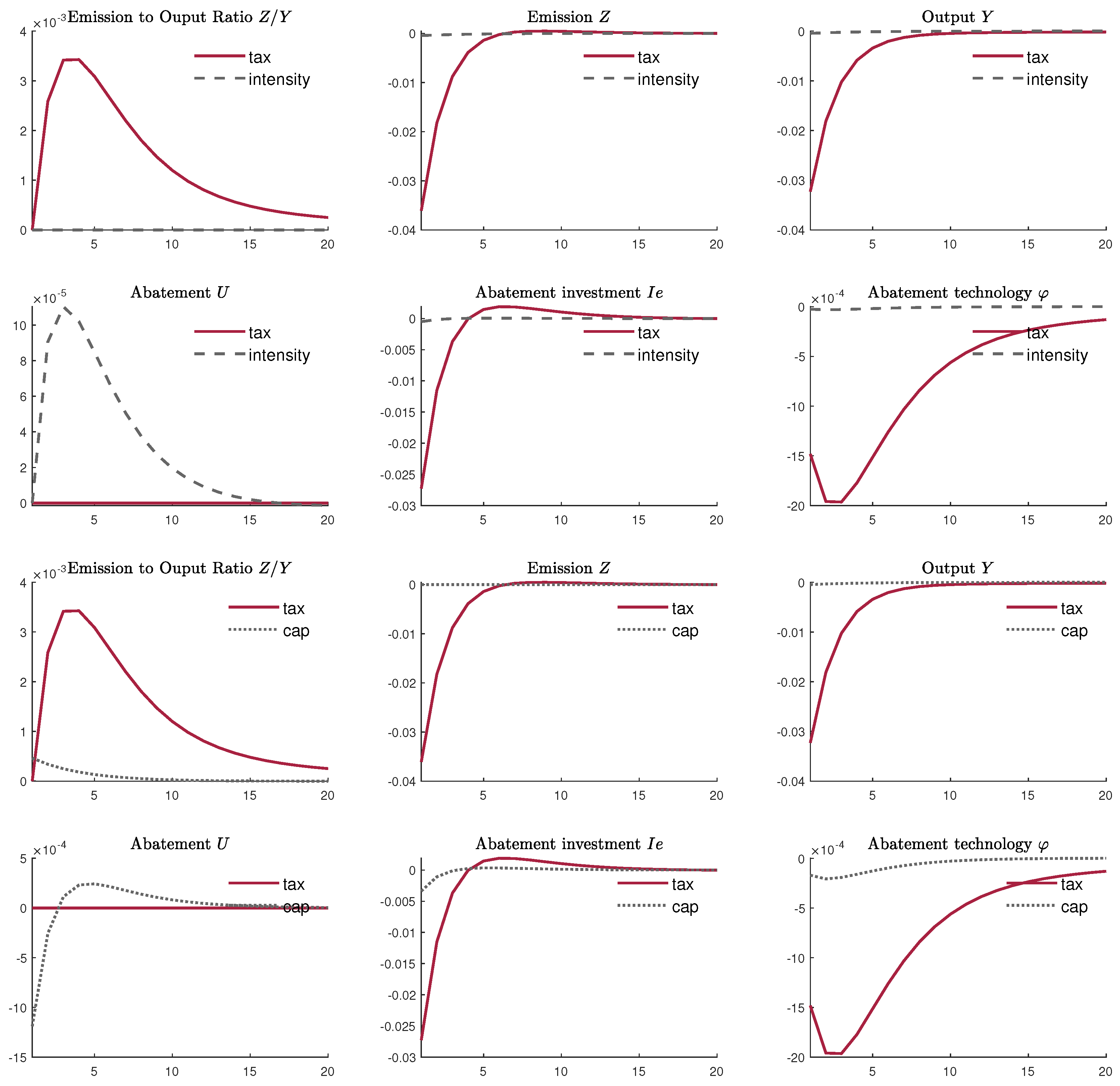
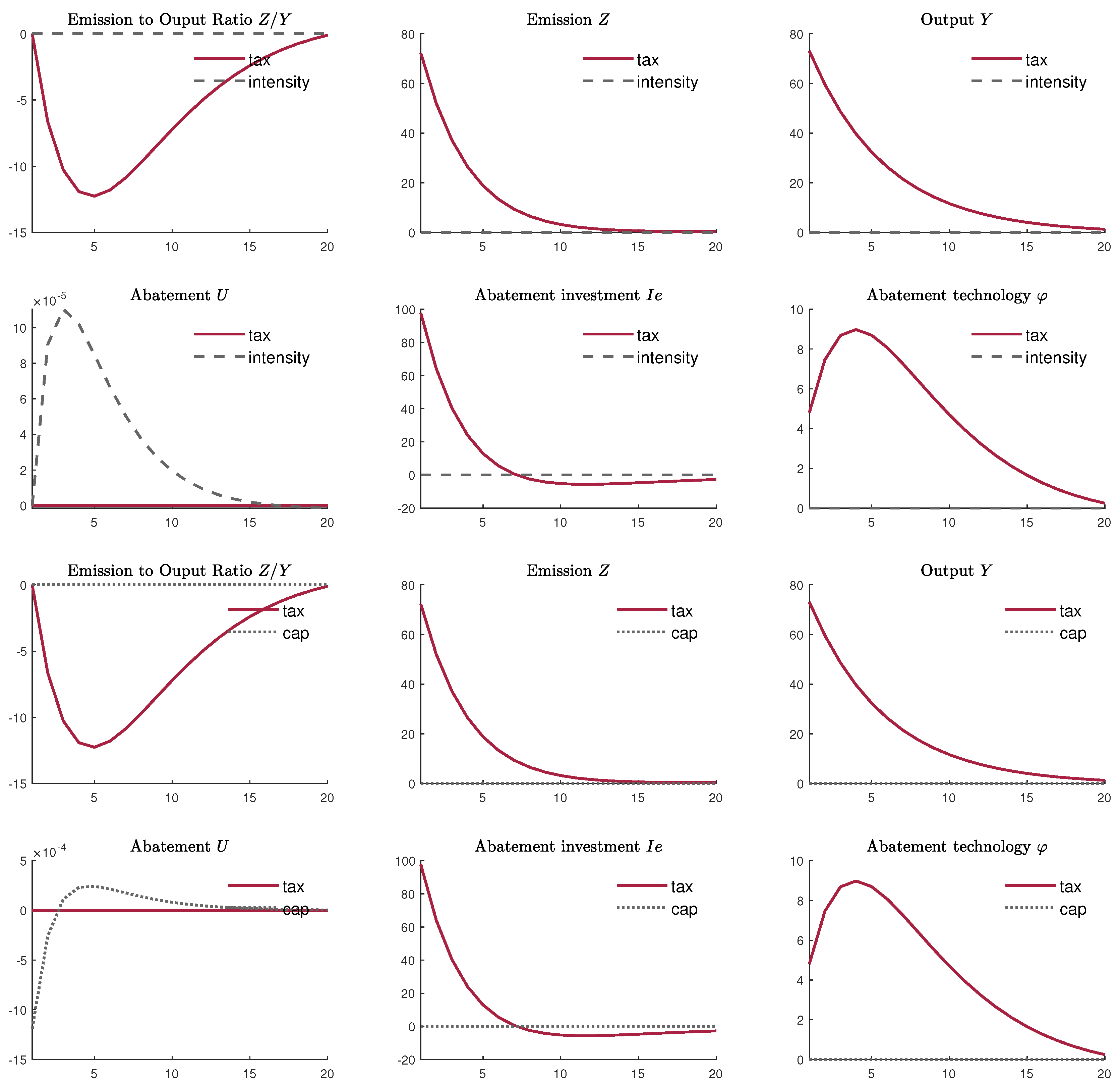
Figure 1 plots the IRFs of our targeted variables to one standard deviation of TFP volatility shocks. The solid lines are the IRFs under a constant carbon tax rate, while the dashed lines in the upper and lower panels are, respectively, the IRFs under carbon intensity and capacity regimes. For the carbon tax regime, the primary effect of a positive TFP uncertainty shock is to reduce the firms’ expected value of future output. The lower expected future output discourages firms’ abatement investment; thus, $I_t^e$ falls initially. With the constant abatement effort fixed by the constant carbon tax rate, the carbon intensity is entirely determined by the abatement technology ${\phi }_t$. The lower abatement investment is accompanied by a lower level of abatement technology, and therefore the IRF of carbon intensity $Z_t/Y_t$ is above zero over time. Likewise, capital investment also decreases, so lower capital is accumulated. As a result, both the output and CO${}_2$ emissions decrease.

Note that both the increase in the emission to output ratio $Z_t/Y_t$ and the decrease in the abatement efficiency brought out by the TFP uncertainty shock could be unfavorable to the economy. Can this be solved by an intensity policy where the ratio $Z_t/Y_t$ is restricted to a certain level? According to the dashed line in the upper panels of Figure 1, with such a policy, $Z_t/Y_t$ is constant over time. CO${}_2$ emissions and output drop to a much lesser extent than those with carbon taxation. As the carbon intensity is required to be constant, firms cannot reduce the abatement investment as much as in the taxation scenario. The abatement investment and hence abatement technology reduce slightly. As mentioned in Section 3.5, the firms face a trade-off between the abatement investment and abatement effort decision under a carbon intensity regime. Firms would exert more abatement effort in response to the slight decrease in abatement investment. In sum, unlike under the carbon taxation regime where output would decrease in response to a positive TFP volatility shock, output can be maintained at a relatively stable level under the carbon intensity regime. However, as the firms are required to maintain the carbon intensity level, they cannot cut off their operating cost and hence are expected to earn less than those under the taxation regime.

The bottom panels of Figure 1 compare the IRFs under the carbon capacity and taxation policies. Clearly, the emission level does not respond to the TFP volatility shock under the capacity regime. Naturally, this implies that the output is allowed to drop slightly. As a result, the carbon intensity level increases to a much lesser extent. Likewise, the dampened rise of carbon intensity restricts the firms to only have a minor reduction in abatement investment. Hence, the responses of abatement investment and abatement technology are much stable under this regime. Complement to the decrease in abatement investment, abatement effort also decreases slightly. To conclude, similar to the carbon intensity regime, a carbon capacity regime could stabilize the responses of carbon emissions, carbon intensity, and output level to the TFP volatility shock. While different from the carbon intensity regime, abatement effort decreases in response to the shock.

4.2.2. Preference Volatility Shock

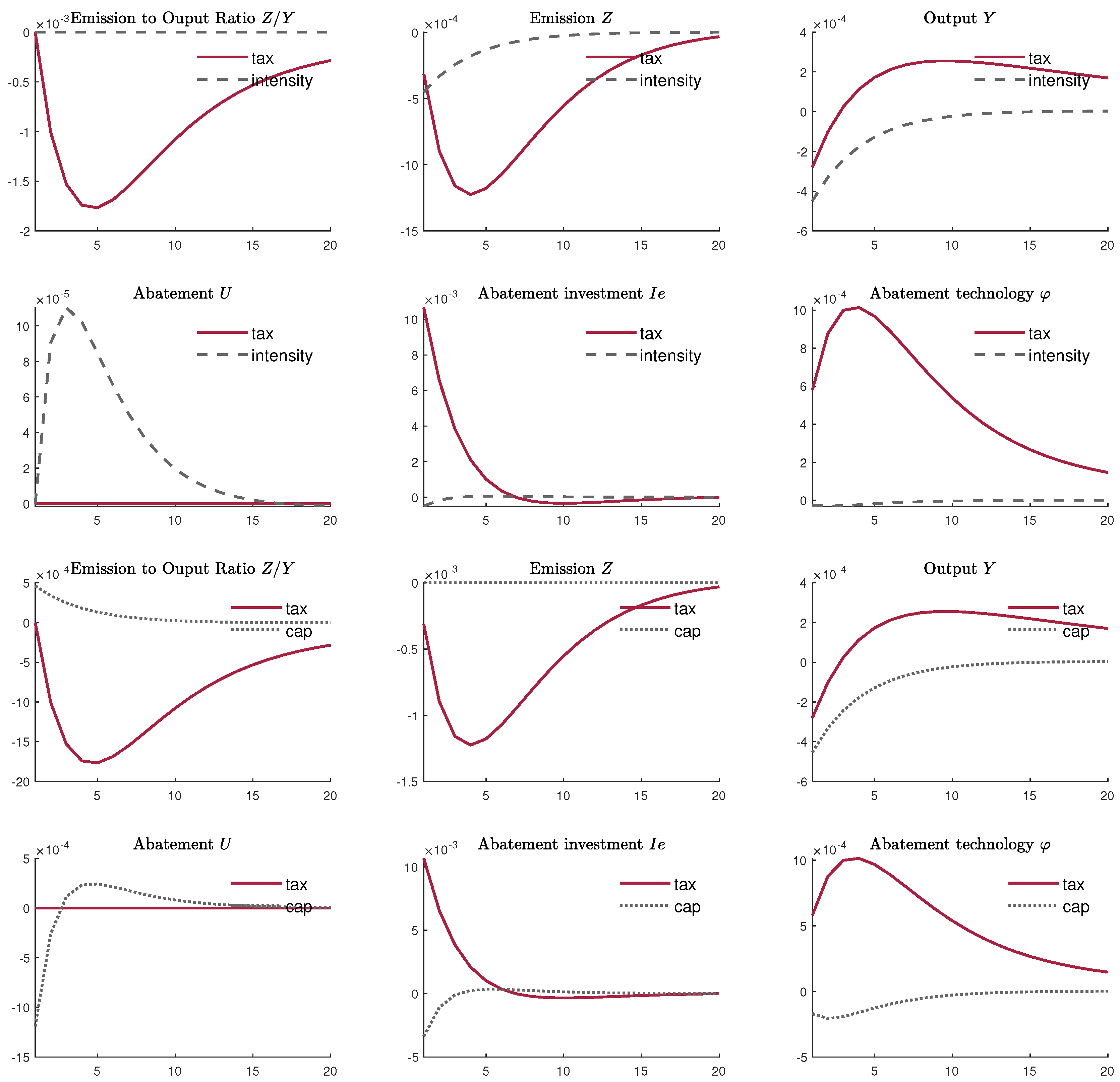
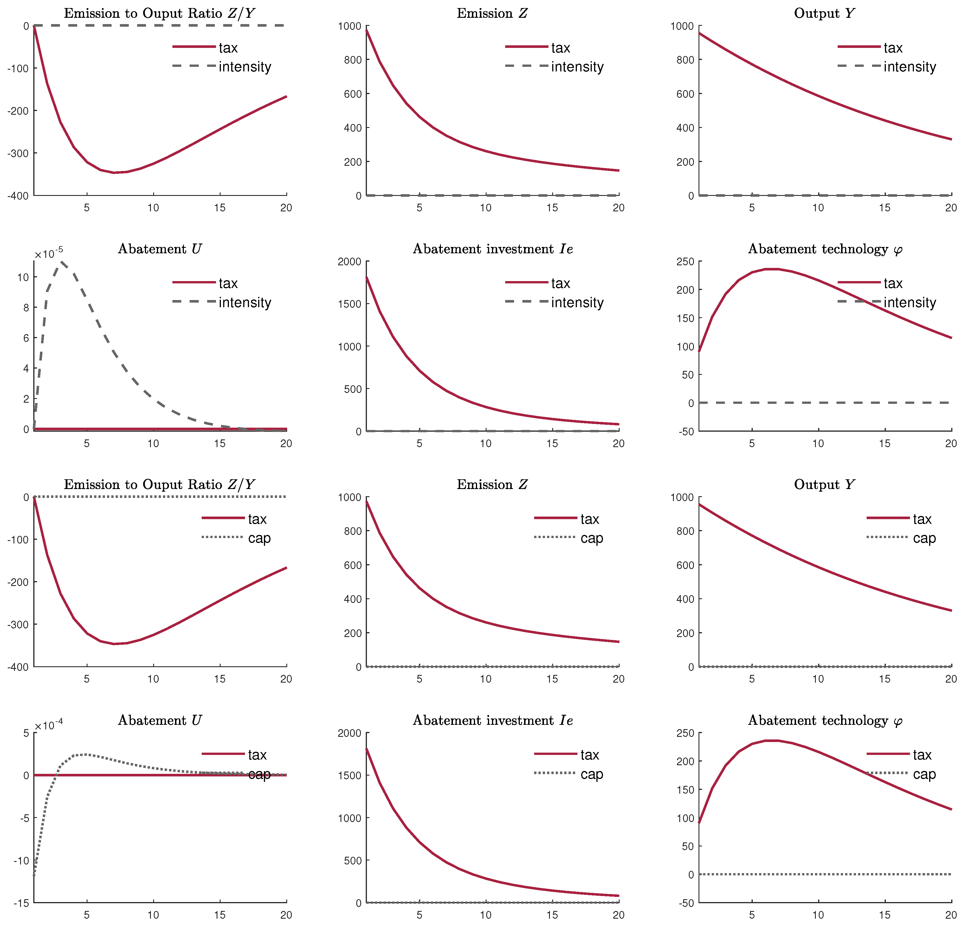
The TFP uncertainty shock mainly captures the sudden change in the uncertainty factors that emerged from the good supply; the uncertainty from the good demand is examined in this subsection. Figure 2 plots the IRFs to one standard deviation increase in the volatility of preference shock. As the preference shock $a_t$ is attached to the value function (1), an increase in the volatility of $a_t$ leads to a more dispersed future value $V_{t+s}$. Thus, the primary effect of an increase in preference uncertainty is the decline in the expected future value ${\mathbb{E}}_t\left[V_{t+s}^{1-\sigma }\right]$. According to Equation (11), the stochastic discount factor increases due to the decrease of ${\mathbb{E}}_t\left[V_{t+s}^{1-\sigma }\right]$. That is, the household has a higher marginal value to consume in the future compared to the current one. As a result, the household saves more due to the precautionary motive, and the current consumption drops. As shown in Figure 2, a lower consumption would naturally lead to a lower output level initially. Over time, the output increases gradually as household becomes wealthier.

From the firms’ perspective, the increase in the stochastic discount factor means that the firms are more concerned about the future profits, as seen from the formula of the firms’ profit function (24). Firms find them optimal to have more abatement investment; thus, Figure 2 shows an initial surge in $I_t^e$ under a constant carbon tax rate. Such an increase in $I_t^e$ is able to compensate for the abatement technology depreciation, leading to the rise in the abatement technology in the first few periods. Over time, the fall in abatement investment is accompanied by the decline in abatement technology, and both of them depreciate gradually back to their steady-state levels. As the abatement effort is fixed under the constant carbon tax rate, carbon intensity $Z_t/Y_t$ is solely a function of abatement technology. Thus, the hump-shaped path of the abatement technology is translated to the U-shaped path of the carbon intensity. As the magnitude of the decline in output is less than those of the carbon intensity, emission level $Z_t$ also exhibits a U-shape. Compared to the IRFs of TFP uncertainty shock under constant carbon tax rate, the main difference here is the rise in abatement investment and technology, as well as the fall in carbon intensity. This reveals that uncertainty shock does not necessarily discourage the firms from abatement investment. Under a preference uncertainty shock, the increase in the stochastic discount factor not only arouses the precautionary motive of the household, but also make the firms discount less of their future profits. As a result, environmental degradation could be mitigated due to the rise in the abatement investment. In sum, both the positive TFP and preference uncertainty shocks would reduce the CO${}_2$ emission level, consistent with the procyclical CO${}_2$ emission cycles as observed from the data, but they create an opposite impact on the carbon intensity and abatement investment.

For the intensity regime, it can be seen from the upper panels of Figure 2 that both the carbon intensity and emission level are stable, compared to the paths under the constant tax rate. Although the output falls slightly more under carbon intensity regime, the drop in the emission level is more dramatic under carbon tax policy. Unlike the case of the carbon tax rate policy that firms can earn a higher profit by reducing the future emission level in order to pay a lower carbon tax, the intensity regime does not create such an incentive for them to reduce the future emission level, even if they have a higher stochastic discount factor. Firms, thus, do not have the incentive to invest more in abatement or exert more abatement effort once the intensity target is met. Therefore, the abatement investment does not respond to the preference shock substantially, and the abatement effort only increases by a very small amount.

Similar logic can be applied to explain the IRFs under the capacity regime. From the lower panels of Figure 2, emission and intensity levels are quite stable over time. Although the emission level is required to be fixed, the intensity level only decreases slightly over time, due to the stable abatement investment and technology. Firms are not willing to invest more in abatement technology as long as the capacity target is satisfied. With a fall in output, the firms can easily meet the capacity target with the same abatement effort and investment. To cut cost, firms would reduce the abatement effort and investment simultaneously.

4.3. Discussion

After examining the IRFs of variables to the uncertainty shocks arising from the good demand and supply sides under the three carbon policies, we find that which policy is the best depends on the type of uncertainty shock realized.

Table 3. Initial responses of the equilibrium values of variables under different carbon policies in the presence of positive TFP and preference uncertainty shocks. The signs ↑ and ↓, −, respectively, indicate that variable increases or decreases remain constant. In each column, ↑↑ and ↓↓, respectively, indicate that the corresponding variable increases or decreases dramatically more than the other policies.

TFP uncertainty shock	${\mathit{I}}_{\mathit{t}}^{\mathit{e}}$	${\mathit{Z}}_{\mathit{t}}$	$\frac{{\mathit{Z}}_{\mathit{t}}}{{\mathit{Y}}_{\mathit{t}}}$	${\mathit{Y}}_{\mathit{t}}$	${\mathit{U}}_{\mathit{t}}$
Carbon tax	↓↓	↓↓	↑↑	↓↓	−
Intensity	↓	↓	−	↓	↑
Capacity	↓	−	↑	↓	↓
Preference uncertainty shock	${\mathit{I}}_{\mathit{t}}^{\mathit{e}}$	${\mathit{Z}}_{\mathit{t}}$	$\frac{{\mathit{Z}}_{\mathit{t}}}{{\mathit{Y}}_{\mathit{t}}}$	${\mathit{Y}}_{\mathit{t}}$	${\mathit{U}}_{\mathit{t}}$
Carbon tax	↑	↓↓	↓↓	↓	−
Intensity	↓	↓	−	↓↓	↑
Capacity	↓	−	↓	↓↓	↓

summarizes the initial changes of the key variables under the three policies with TFP and preference uncertainty shocks. As shown, measuring in term of output, both the intensity and capacity regimes are preferable to the constant tax rate under a TFP uncertainty shock. In contrast, under a preference uncertainty shock, implementing a carbon tax rate can reduce the extent of reduction of output, relatively to the other two policies. This is in contrast to the result found by Annicchiarico and Di Dio [13] and Dissou and Karnizova [15], where the capacity regime could dampen the responses of macroeconomic variables to the level shocks. This result no longer holds under uncertainty shocks.

Regarding the choice between the constant carbon tax rate and intensity regime, if the policy-maker’s objective is to reduce both the emission and intensity levels in responding to economic uncertainty, carbon intensity is preferable to the taxation regimes under a TFP uncertainty shock. This is because although the carbon tax policy could lead to relatively more reduction in CO${}_2$ emissions, it substantially increases the carbon intensity level, which is caused by the large reduction in the abatement investment under the policy. In contrast, the constant carbon tax rate seems to be more preferable under a positive preference uncertainty shock. This outcome occurs because, as shown in Figure 2, with a constant carbon tax rate, both the carbon intensity and emission levels fall in response to the preference uncertainty shock, whereas their paths are more stable under the carbon intensity regime. The environmental condition can be enhanced by the rise in abatement investment under a constant carbon tax rate in the presence of a higher preference uncertainty shock that increases the stochastic discount factor.

Regarding the choice between the carbon tax rate and capacity regimes, the capacity regime is more preferable under a TFP uncertainty shock. AS abatement effort and investment can be chosen freely under the capacity regime, the abatement investment decreases to a lesser extent under the policy. As a result, the carbon intensity ratio does not increase as much as those under the constant carbon tax rate. Facing a preference volatility shock, the emission and intensity levels under the capacity regime behave similarly to those under the intensity regime. Both paths move steadily over time. Even worse, the abatement effort is reduced under the capacity regime. Thus, the carbon tax rate is more preferable under the preference uncertainty shock.

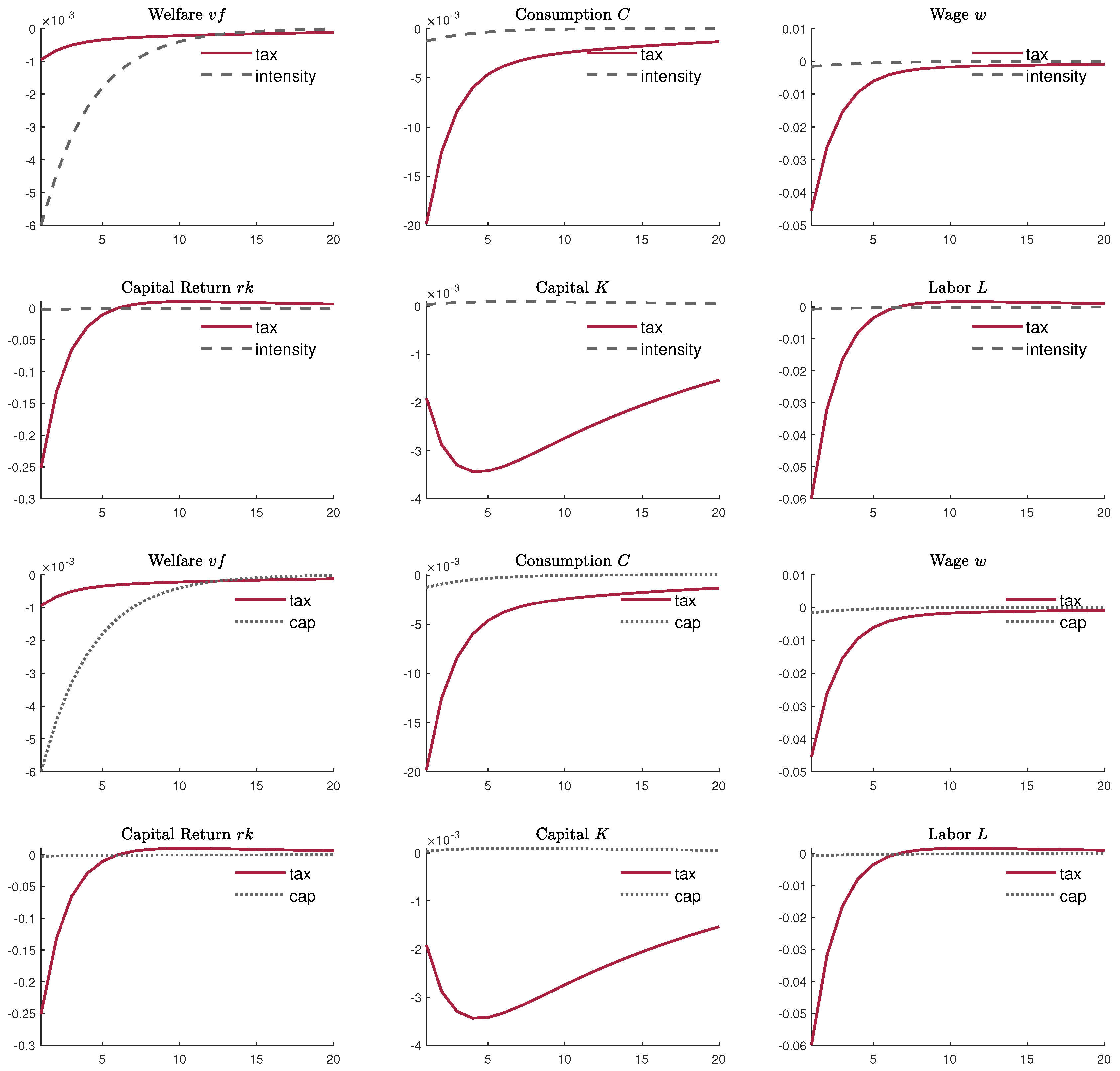
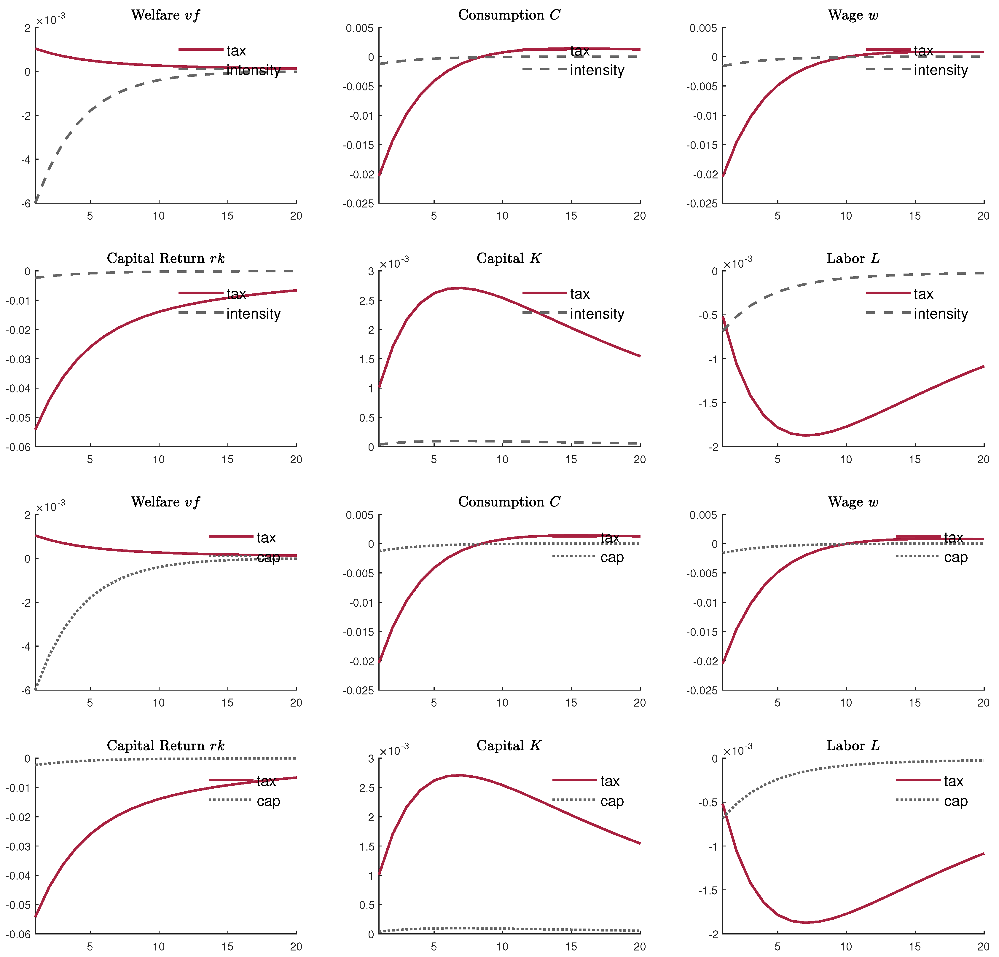
In sum, the constant carbon tax rate is the best policy in term of output, emissions and intensity level under the preference volatility shock. However, the intensity and capacity regimes are more preferable under the TFP volatility shock. In the standard literature in macroeconomics, usually, one only takes the household’s utility (1) into consideration for the welfare analysis and neglects the adverse impact on the environment. In Appendix C, we show the IRFs of the other variables to the uncertainty shocks. It is shown that the constant carbon tax rate produces a higher household lifetime utility than the other two policies under both types of shocks.

5. Conclusions and Extensions

This paper studies the impact of the economic uncertainty on the carbon emissions, and the welfare consequences of the carbon tax, intensity, and capacity regimes. Our DSGE model is a combination of the models by Annicchiarico and Di Dio [13], Heutel [14], and Basu and Bundick [12], and features environmental components as well as the uncertainty shocks from the good supply (TFP uncertainty shock) and demand (preference uncertainty shock). It is found that an increase in uncertainty from both sources can reduce CO${}_2$ emissions. However, their impacts on the abatement investment are different: a positive TFP uncertainty shock results in a lower abatement investment through reducing the future expected productivity level, whereas a positive preference uncertainty shock increases the abatement investment by raising the stochastic discount factor.

It is worth noting that carbon tax, intensity, and capacity policies yield vastly different welfare implications in response to the uncertainty shocks. In terms of lifetime utility, the carbon tax policy is the most preferable under both types of the uncertainty shocks. In terms of output, it is the most preferable only under the preferable uncertainty shock; whereas, instead, the intensity and capacity regimes should be implemented under the TFP uncertainty shock.

Speaking of the carbon emissions and intensity levels, the welfare implication is mixed. A unique feature of implementing a carbon tax policy is fixing the abatement effort at a constant level, leaving the abatement investment to be the only tool for firms to manipulate the emission level. As a result, the abatement investment would increase and decrease, respectively, to positive preference and TFP shocks. Thus, to mitigate both the carbon emissions and intensity levels, the carbon tax regime is suitable only under the preference shock. In contrast, the carbon intensity regime results in a trade-off between the abatement effort and abatement investment. The abatement investment and abatement effort are determined before and after the realization of the shocks, respectively, and the firms would overinvest if their realized intensity levels are below the required one. In this context, the possibility of overinvestment leads to a reduction in the firms’ abatement investment under a positive TFP uncertainty shock. In line with Baldursson and Von Der Fehr [32], the irreversible property of investment is the key for the uncertainty shock to take impacts. Since the abatement investment (and abatement effort) are insensitive to both types of the uncertainty shocks, the abatement technology decreases to a lesser extent under the TFP uncertainty shock. Therefore, the carbon intensity regime is preferable to the carbon tax regime under the TFP uncertainty shock.

Under the capacity regime, the abatement investment decreases under both types of the uncertainty shocks. This is because both of the uncertainty shocks reduce output, and the carbon emissions decrease naturally without requiring further actions in abatement. Firms that find it easier to satisfy the capacity target, tend to invest less and exert less effort in abatement. Similar to the intensity regime, the abatement investment is insensitive to the shock under the capacity regime, therefore the social welfare under these two regimes (in term of carbon emission and intensity levels) are similar. To conclude, in order to curb environmental degradation in terms of the CO${}_2$ emission and intensity levels under economic uncertainty, we show that the intensity and capacity regimes are more suitable when facing the TFP uncertainty shocks, whereas the carbon tax policy is the most suitable policy when facing the preference uncertainty shock.

Another branch of the economic uncertainty literature is to study the macroeconomic impact of policy uncertainty. For example, Fernández-Villaverde et al. [28] found that high volatility of interest rate could result in decreases in output and consumption in a partial equilibrium small open economy model. When facing a higher interest rate uncertainty, households hold less foreign bonds. As holding foreign bonds allow the households to hedge against the risk of investing in physical capital, a reduction in foreign bonds also implies that less real investment is made. A similar result is also obtained by Mumtaz and Zanetti [33] who use a structural vector autoregression model to show that a rise in monetary policy volatility could trigger falls in the interest rate, output growth rate, and inflation rate. In a New Keynesian model with time-varying volatility of government expenditure, Fernández-Villaverde et al. [34] found that the fiscal policy uncertainty could at least reduce the output in the U.S. by 0.15%. Moreover, firms with higher productivity uncertainty are more vulnerable to such fiscal policy uncertainty [35]. To quantify the degree of policy uncertainty, Baker et al. [36] measure it by counting the frequency of the words “uncertainty” in the articles of ten leading U.S. newspapers. This index is employed by Kang and Ratti [37] and Antonakakis et al. [38], who find a dynamic relationship between policy uncertainty and oil prices. Both papers find a significant and positive relationship between an oil-specific demand shock and the policy uncertainty index, whereas oil supply shock is loosely linked to the index. In addition to monetary and fiscal policies, Handley and Limao [39] found that a high uncertainty in trade policy (tariff rate) can also reduce firms’ investment and the probability to enter the export market. One might wonder whether the uncertainty in the future implementation of carbon policies could also lead to a similar result. In addition, it is also interesting to examine the environmental impact of fiscal and monetary uncertainty, all of which we leave for future research.

References

- Bloom, N. The impact of uncertainty shocks. Econometrica 2009, 77, 623–685. [Google Scholar]
- Bloom, N. Fluctuations in uncertainty. J. Econ. Perspect. 2014, 28, 153–176. [Google Scholar] [CrossRef]
- Knight, F.H. Risk, Uncertainty and Profit; Augustus Kelley: New York, NY, USA, 1921. [Google Scholar]
- Bloom, N.; Floetotto, M.; Jaimovich, N.; Saporta-Eksten, I.; Terry, S.J. Really uncertain business cycles. Econometrica 2018, 86, 1031–1065. [Google Scholar] [CrossRef]
- Bulan, L.T. Real options, irreversible investment and firm uncertainty: new evidence from US firms. Rev. Financ. Econ. 2005, 14, 255–279. [Google Scholar] [CrossRef]
- Bachmann, R.; Bayer, C. ‘Wait-and-See’business cycles? J. Monet. Econ. 2013, 60, 704–719. [Google Scholar] [CrossRef]
- Guiso, L.; Parigi, G. Investment and demand uncertainty. Q. J. Econ. 1999, 114, 185–227. [Google Scholar] [CrossRef]
- Baum, C.F.; Caglayan, M.; Talavera, O. Uncertainty determinants of firm investment. Econ. Lett. 2008, 98, 282–287. [Google Scholar] [CrossRef] [Green Version]
- Panousi, V.; Papanikolaou, D. Investment, idiosyncratic risk, and ownership. J. Financ. 2012, 67, 1113–1148. [Google Scholar] [CrossRef]
- Leahy, J.V.; Whited, T.M. The Effect of Uncertainty on Investment: Some Stylized Facts. J. Money Credit. Bank. 1996, 28, 64–83. [Google Scholar] [CrossRef]
- Novy, D.; Taylor, A.M. Trade and Uncertainty; Technical Report; National Bureau of Economic Research: Cambridge, MA, USA, 2014. [Google Scholar]
- Basu, S.; Bundick, B. Uncertainty shocks in a model of effective demand. Econometrica 2017, 85, 937–958. [Google Scholar] [CrossRef]
- Annicchiarico, B.; Di Dio, F. Environmental policy and macroeconomic dynamics in a new Keynesian model. J. Environ. Econ. Manag. 2015, 69, 1–21. [Google Scholar] [CrossRef] [Green Version]
- Heutel, G. How should environmental policy respond to business cycles? Optimal policy under persistent productivity shocks. Rev. Econ. Dyn. 2012, 15, 244–264. [Google Scholar] [CrossRef] [Green Version]
- Dissou, Y.; Karnizova, L. Emissions cap or emissions tax? A multi-sector business cycle analysis. J. Environ. Econ. Manag. 2016, 79, 169–188. [Google Scholar] [CrossRef] [Green Version]
- Jurado, K.; Ludvigson, S.C.; Ng, S. Measuring uncertainty. Am. Econ. Rev. 2015, 105, 1177–1216. [Google Scholar] [CrossRef]
- Berger, D.; Vavra, J.S. Volatility and Pass-Through; Technical Report; National Bureau of Economic Research: Cambridge, MA, USA, 2013. [Google Scholar]
- Kehrig, M. The Cyclical Nature of the Productivity Distribution; Earlier Version; US Census Bureau Center for Economic Studies: Washington, DC, USA, 2015; Paper No. CES-WP-11-15.
- Gourio, F. Disaster risk and business cycles. Am. Econ. Rev. 2012, 102, 2734–2766. [Google Scholar] [CrossRef]
- Punzi, M.T. The impact of energy price uncertainty on macroeconomic variables. Energy Policy 2019, 129, 1306–1319. [Google Scholar] [CrossRef]
- Hassler, J.; Krusell, P.; Smith, A.A., Jr. Environmental macroeconomics. In Handbook of Macroeconomics; Elsevier: Amsterdam, The Netherlands, 2016; Volume 2, pp. 1893–2008. [Google Scholar]
- Fischer, C.; Springborn, M. Emissions targets and the real business cycle: Intensity targets versus caps or taxes. J. Environ. Econ. Manag. 2011, 62, 352–366. [Google Scholar] [CrossRef]
- Farmer, J.D.; Hepburn, C.; Mealy, P.; Teytelboym, A. A third wave in the economics of climate change. Environ. Resour. Econ. 2015, 62, 329–357. [Google Scholar] [CrossRef]
- Lucas, R. Econometric policy evaluation: A critique. In Carnegie-Rochester Conference Series on Public Policy; North-Holland: Amsterdam, The Netherlands, 1976; Volume 1, pp. 19–46. [Google Scholar]
- De Groot, O.; Richter, A.W.; Throckmorton, N.A. Uncertainty Shocks in a Model of Effective Demand: Comment. Econometrica 2018, 86, 1513–1526. [Google Scholar] [CrossRef] [Green Version]
- Christiano, L.J.; Motto, R.; Rostagno, M. Risk shocks. Am. Econ. Rev. 2014, 104, 27–65. [Google Scholar] [CrossRef]
- Fernald, J. A Quarterly, Utilization-Adjusted Series on Total Factor Productivity; Federal Reserve Bank of San Francisco: San Francisco, CA, USA, 2014. [Google Scholar]
- Fernández-Villaverde, J.; Guerrón-Quintana, P.; Rubio-Ramírez, J.F.; Uribe, M. Risk matters: The real effects of volatility shocks. Am. Econ. Rev. 2011, 101, 2530–2561. [Google Scholar] [CrossRef]
- Kim, J.; Kim, S.; Schaumburg, E.; Sims, C.A. Calculating and using second-order accurate solutions of discrete time dynamic equilibrium models. J. Econ. Dyn. Control. 2008, 32, 3397–3414. [Google Scholar] [CrossRef] [Green Version]
- Andreasen, M.M.; Fernández-Villaverde, J.; Rubio-Ramírez, J.F. The pruned state-space system for non-linear DSGE models: Theory and empirical applications. Rev. Econ. Stud. 2017, 85, 1–49. [Google Scholar] [CrossRef]
- Lan, H.; Meyer-Gohde, A. Pruning in Perturbation DSGE Models-Guidance from Nonlinear Moving Average Approximations; Technical Report; Sonderforschungsbereich 649, Humboldt University: Berlin, Germany, 2013. [Google Scholar]
- Baldursson, F.M.; Von Der Fehr, N.H.M. Prices vs. quantities: The irrelevance of irreversibility. Scand. J. Econ. 2004, 106, 805–821. [Google Scholar] [CrossRef]
- Mumtaz, H.; Zanetti, F. The impact of the volatility of monetary policy shocks. J. Money Credit. Bank. 2013, 45, 535–558. [Google Scholar] [CrossRef]
- Fernández-Villaverde, J.; Guerrón-Quintana, P.; Kuester, K.; Rubio-Ramírez, J. Fiscal volatility shocks and economic activity. Am. Econ. Rev. 2015, 105, 3352–3384. [Google Scholar] [CrossRef]
- Kang, W.; Lee, K.; Ratti, R.A. Economic policy uncertainty and firm-level investment. J. Macroecon. 2014, 39, 42–53. [Google Scholar] [CrossRef] [Green Version]
- Baker, S.R.; Bloom, N.; Davis, S.J. Measuring economic policy uncertainty. Q. J. Econ. 2016, 131, 1593–1636. [Google Scholar] [CrossRef]
- Kang, W.; Ratti, R.A. Structural oil price shocks and policy uncertainty. Econ. Model. 2013, 35, 314–319. [Google Scholar] [CrossRef] [Green Version]
- Antonakakis, N.; Chatziantoniou, I.; Filis, G. Dynamic spillovers of oil price shocks and economic policy uncertainty. Energy Econ. 2014, 44, 433–447. [Google Scholar] [CrossRef] [Green Version]
- Handley, K.; Limao, N. Trade and investment under policy uncertainty: Theory and firm evidence. Am. Econ. J. Econ. Policy 2015, 7, 189–222. [Google Scholar] [CrossRef]
Figure 1.
Impulse response functions (IRFs) to one standard deviation of total factor productivity (TFP) uncertainty shock. The values of IRFs are all expressed in percent. In the upper six panels, the solid lines represent the IRFs when the carbon tax . The dashed lines are the IRFs under the carbon intensity policy. The intensity policy is set such that the ratios are equal in the two models in the steady state. For the bottom six panels, the solid lines represent the IRFs when the carbon tax . The dotted lines are the IRFs under the carbon capacity policy, such that the emission levels are equal in the two models in the steady state.
Figure 2.
Impulse response functions (IRFs) to one standard deviation of preference uncertainty shock. The values of IRFs are all expressed in percent. In the upper six panels, the solid lines represent the IRFs when the carbon tax . The dashed lines are the IRFs under the carbon intensity policy. The intensity policy is set such that the ratios are equal in the two models in the steady state. For the bottom six panels, the solid lines represent the IRFs when the carbon tax . The dotted lines are the IRFs under the carbon capacity policy, such that the emission levels are equal in the two models in the steady state.