Analysis of Land Surface Deformation in Chagan Lake Region Using TCPInSAR


1
College of Geo-Exploration Science and Technology, Jilin University, Changchun 130026, China
2
Department of Land Surveying and Geo-Informatics, The Hong Kong Polytechnic University, Hong Kong 999077, China
3
College of Construction Engineering, Jilin University, Changchun 130026, China
*
Authors to whom correspondence should be addressed.
Sustainability 2019, 11(18), 5090; https://0-doi-org.brum.beds.ac.uk/10.3390/su11185090
Submission received: 2 August 2019
/
Revised: 3 September 2019
/
Accepted: 14 September 2019
/
Published: 17 September 2019
(This article belongs to the Special Issue Sustainable Applications of Remote Sensing and Geospatial Information Systems to Earth Observations)
Abstract
:Due to earthquakes and large-scale exploitation of oil, gas, groundwater, and coal energy, large-scope surface deformation has occurred in Songyuan City, Jilin Province, China, and it is posing a serious threat to sustainable development, including urban development, energy utilization, environmental protection, and construction to improve saline–alkali land. In this study, we selected the Chagan Lake region, which is located in Songyuan City, as our research area. Using temporarily coherent point synthetic aperture radar interferometry (TCPInSAR), we obtained a time series of land surface deformation and the deformation rate in this area from 20 ALOS PALSAR images from 2006 to 2010. The results showed that the deformation rate in the Chagan Lake region ranged from −46.7 mm/year to 41.7 mm/year during the monitoring period. In three typical land cover areas of the Chagan Lake region, the subsidence in the wetland area was larger than that in the saline–alkali area, while the highway experienced a small uplift. In addition, surface deformation in lakeside areas with or without dykes was different; however, as this was mainly affected by soil freeze–thaw cycles and changes in groundwater level, the deformation showed a negative correlation with temperature and precipitation. By monitoring and analyzing surface deformation, we can provide a data reference and scientific basis for sustainable ecological and economic development in the Chagan Lake region and adjacent areas.
1. Introduction
Surface deformation manifests as land subsidence (due to groundwater or oil and gas exploitation, a mining area collapse, etc.), landslides, glacial flows, active volcanic uplift or sinking, crustal fault movements, etc. These surface deformation phenomena are closely related to sustainable development issues, such as urban planning, economic development, and geological hazard prevention and control, so it is particularly important to continuously monitor surface deformation. At present, the traditional methods that are commonly used to monitor land surface deformation include leveling, GPS, etc. [1,2,3]. However, these traditional monitoring methods have some shortcomings, such as being time-consuming, laborious, high-cost, slow to update data, and limited in monitoring scope, that make it difficult to use them to meet the scale and timeliness requirements of surface deformation monitoring at present.
As satellite earth observation technology has become more mature, synthetic aperture radar interferometry (InSAR) has been further developed [4,5]. InSAR technology plays an important role in monitoring surface deformation caused by energy exploitation, climate change, volcanic movement, glacier drifts, landslides, earthquakes, etc., and can make up for the shortcomings of the low resolution of traditional methods [6,7,8,9]. Compared to traditional deformation monitoring methods, such as leveling and GPS, InSAR has the advantages of high accuracy, a wide range, all-day operation, and a lesser influence of climate conditions on the observation results. Standard InSAR technology is based on the information that two SAR images in the same region provide for interferometric processing, and information on elevation in the target region can be obtained [10]. Differential InSAR (DInSAR) is a further development of standard InSAR. It uses two SAR images taken at different times in the same area to produce an interferogram by differential interferometry and introduces a digital elevation model to eliminate the influence of terrain factors on the interferogram to obtain information on surface deformation during the acquisition of the two images in the area. DInSAR can supplement the traditional land surface deformation monitoring methods and has some advantages and prospects for application [11,12,13,14]. However, if the tropospheric temperature and humidity change during the acquisition of the two SAR images, the spatial baseline and the change in the scattering characteristics of targets caused by long observation intervals can easily lead to the phenomena of atmospheric phase delay and decorrelation, which can affect the DInSAR monitoring results. Moreover, it is not easy to use DInSAR to obtain time-series deformation monitoring results for the same region, which limits its application to a certain extent.
In order to compensate for the limitations of DInSAR in land surface deformation monitoring, time-series InSAR methods, such as persistent scatter InSAR (PSInSAR) [15,16] and small-baseline subset InSAR (SBAS) [17,18,19], have been proposed. PSInSAR chooses one SAR image as a reference image from N SAR images that cover the same area with different acquisition times, and the rest of the images are used as subimages. Through interference processing, N − 1 interference pairs can be obtained. Target points with a high degree of coherence during the monitoring period (e.g., corners of walls, roofs of buildings, or exposed rocks) are selected as PS points. The effect of atmospheric phase delay is eliminated through a filtering method, the PS points are analyzed by a time series, and then multitemporal surface deformation information is obtained. PSInSAR technology is suitable for monitoring surface deformation in urban areas with a high degree of overall coherence [20,21]. In view of the fact that only one reference image in PSInSAR is prone to spatiotemporal decorrelation, SBAS has made further improvements in this respect. By setting the time and spatial baseline thresholds of the selected interference image pairs, interference pairs based on different reference images that cover the same area can be obtained, and several small baseline subsets can be formed. However, the SBASes used to monitor multitemporal surface deformation are susceptible to atmospheric delay, and a phase unwrapping error can occur in the “island” region [22]. In contrast, temporarily coherent point InSAR (TCPInSAR) [23], which has been developed in recent years, effectively combines the advantages of PSInSAR and SBAS. There is no need to perform phase unwrapping during the solution process, which effectively mitigates the effect of atmospheric delay on the surface deformation results. By choosing shorter time baselines and smaller spatial baselines, more target points can be selected as temporarily coherent points, and then high-resolution deformation monitoring results for the study area can be obtained. The accuracy of the land surface deformation monitoring results that have been obtained using the TCPInSAR method has been verified in volcanic activity monitoring and land subsidence monitoring studies [24,25].
In this paper, we take the Chagan Lake region in Jilin Province, China, as our research area. In view of the fact that there are fewer target points with a high degree of temporal coherence in the Chagan Lake region and that vegetation cover is liable to cause decorrelation in some lakeside areas, we used the TCPInSAR method and L-band ALOS PALSAR images with strong penetration as a data source to monitor land surface deformation in the Chagan Lake region from 2006 to 2010 and analyzed the causes of deformation by combining local meteorological data.
2. Materials and Methods
2.1. Study Area and Experimental Data
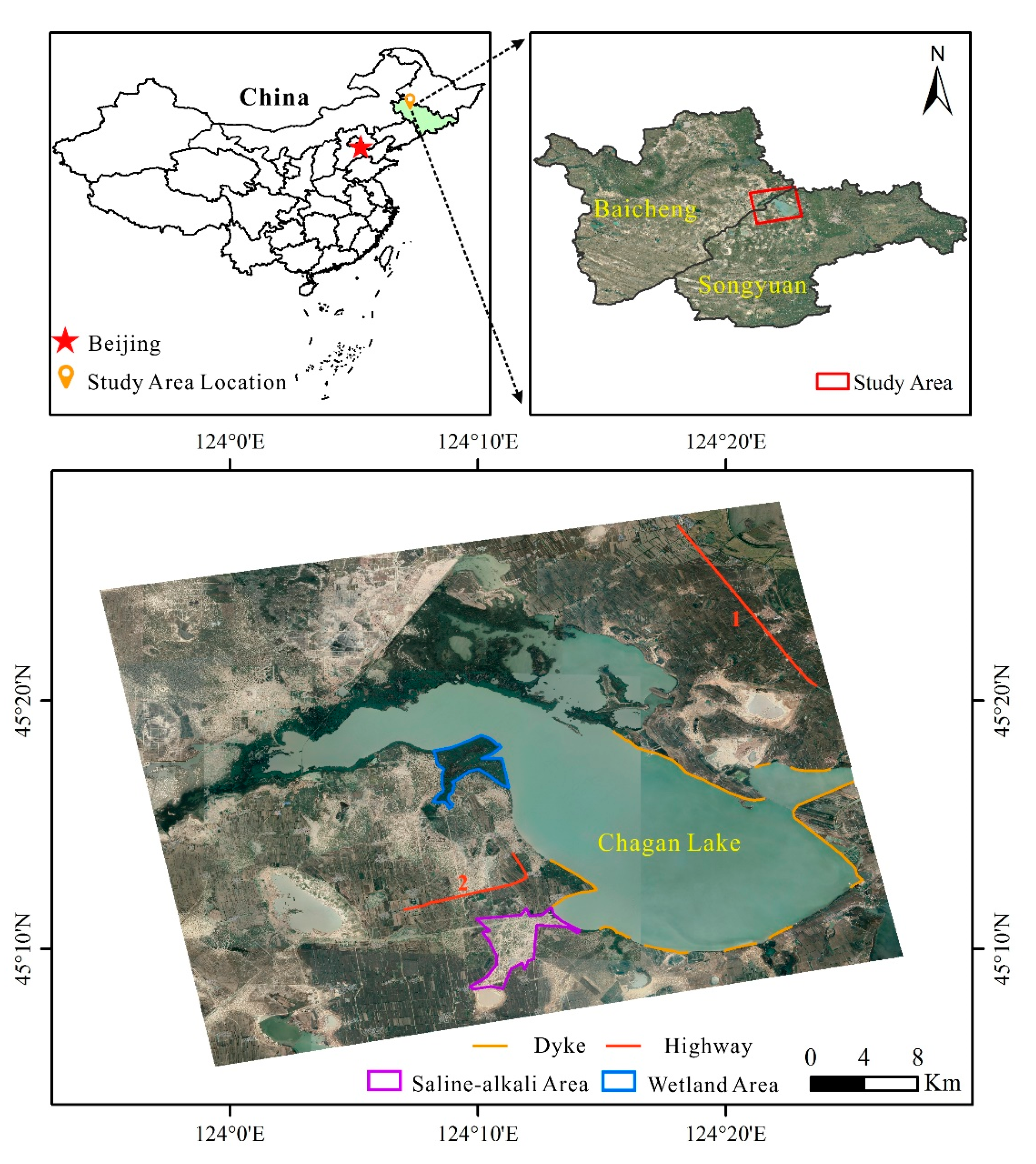
Chagan Lake is the largest natural lake in Jilin Province and has a maximum area of 347.4 square kilometers. It is located in Songyuan City and Baicheng City, western Jilin Province. It contains an abundance of water and fishery resources [26]. However, the land cover of the Chagan Lake region is complex, as there are large areas of saline land and wetland [27]. The water storage in the lake and the climate conditions vary significantly with the seasons. Besides this, the land in the Chagan Lake region is affected by freeze–thaw cycles, earthquakes, and mineral exploitation all year long, and the surface is prone to deformation, which may cause damage to roads and electricity, hydraulics, and other public facilities. This has an impact on the irrigation function of Chagan Lake and on sustainable ecological and economic development in Songyuan City. Therefore, it is necessary to perform long-term monitoring of land surface deformation in the Chagan Lake region [28].
In this study, the Chagan Lake region in Songyuan City and Baicheng City, Jilin Province, China, was selected as the study area, as shown in Figure 1. Chagan Lake extends from the southeast to the northwest and has a narrow overall shape. It is located at the junction of Heilongjiang Province, Jilin Province, and the Inner Mongolia Autonomous Region and the overlapping areas of the Horqin Grasslands, the Songnen Plain, and the Northeast Plain, where the Nenjiang River and the Songhua River meet. The geographical coordinates of Chagan Lake are 45°09′ N to 45°30′ N and 124°03′ E to 124°34′ E.
Chagan Lake is relatively flat on the whole, with a higher elevation in the southeast region and a lower elevation in the central and northeastern regions. It has a length of approximately 38 km in the east–west direction and 14 km in the north–south direction. It has a circumference of 104.5 km. The lake’s maximum water storage capacity is 415 million m3. The Chagan Lake area has a temperate continental monsoon climate, with an average annual precipitation of 300–500 mm and an average annual temperature of 5–7 °C [29]. The geological conditions of the lakeside are complex, and there are many kinds of landforms. In some areas, there are artificial concrete dykes. In the area without dykes, there is a staggered distribution of saline–alkali land with almost no vegetation cover and wetland with dense vegetation cover.
The experimental data that we selected for this study were PALSAR images of the ALOS satellite, which was launched by the National Space Development Agency (NASDA) of Japan in 2006. The radar is a phased-array L-band synthetic aperture radar with a wavelength of 23.6 cm and a revisit period of 46 days. Compared to C-band images, ALOS PALSAR image can penetrate vegetation better because of the ALOS satellite’s longer band. ALOS PALSAR images are suitable for deformation monitoring in areas with complex topography and landforms [30].
Twenty ALOS PALSAR images that covered the study area from 2006 to 2010 were selected for the experiment. The polarization mode of the images was horizontal–horizontal (HH) polarization. The imaging modes included fine-beam single polarization (FBS) and fine-beam dual polarization (FBD). Table 1 shows the specific parameters.
In addition, a digital elevation model from the shuttle radar topography mission (SRTM DEM) provided by the United States Geological Survey (USGS) with a resolution of 30 m was selected to weaken the influence of the topographic phase on the deformation results during the solution process [31]. Meteorological data provided by the National Oceanic and Atmospheric Administration (NOAA) were combined with the deformation results to determine the influence of temperature and precipitation on the deformation and analyze the causes of deformation [32]. An example of what meteorological data look like is shown in Table 2. The meteorological station that provided the meteorological data is located in the Qianguoerros Mongolian Autonomous County of Songyuan City, approximately 30 km away from Chagan Lake. Its geographical coordinates are 45°04′59″ N and 124°52′01″ E. The temperature that is shown in Table 2 was the average temperature for that month, and the precipitation that is shown in Table 2 was the total precipitation for that month.
2.2. Data Processing Using TCPInSAR
2.2.1. Basic Theory of TCPInSAR
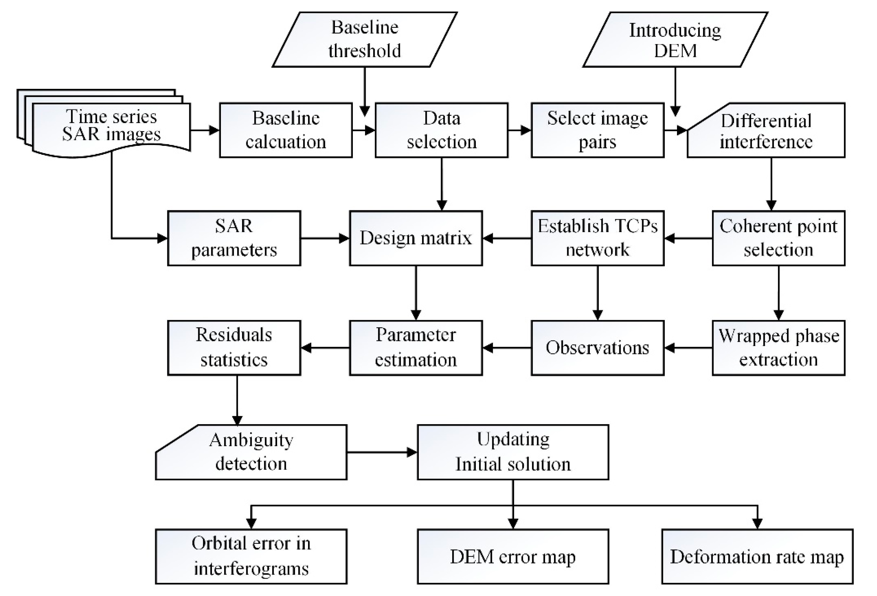
TCPInSAR is a multitemporal InSAR technique that was developed by Hong Kong Polytechnic University’s InSAR Group [33,34,35]. TCPInSAR is characterized by several advanced TCP identifications, TCP networking, and parameter estimation. TCPInSAR distinguishes itself from other methods in two main respects, i.e., its observation model and its parameter estimation. In order to precisely mitigate orbit error and stratified atmospheric delays, TCPInSAR employs a joint model that establishes the relationship between wrapped phases and signals together with parameters of interest. During the parameter estimation stage, by taking phase ambiguities as outliers, TCPInSAR can retrieve deformation parameters without the need for phase unwrapping, which is a challenging and time-consuming task in multitemporal InSAR processing. Figure 2 shows a flowchart on TCPInSAR.
In this section, we introduce the key steps in the TCPInSAR technique that we used to process the ALOS PALSAR images over the Chagan Lake region.
Observations
To reduce decorrelation noise, coherent points in interferograms with short baselines (spatial and temporal baselines and the Doppler centroid difference) were used as observations in the TCPInSAR processor. We then conducted a differential operation among the selected points to generate dense arcs (i.e., coherent point pairs) to reduce the spatially correlated atmospheric signals [36]. Given M differential interferograms generated from N SAR images, the wrapped phase at coherent point p in the ith interferogram can be written as
where W{ } is the wrapping operator; is the phase that is related to the topographic error; is the phase component that is due to ground motion; is the phase that is due to atmospheric delay; is the phase that is due to the orbital error; and is the noise (due mainly to decorrelation effects). For an arc that is constructed by two neighboring coherent points (say, p and q), the phase difference between p and q can be expressed as
If there are G arcs in the ith interferogram, the observations can be written as
The setting vector contains all of the observations of the proposed model, which can be expressed as
Modeling Orbit Errors
We assumed that the orbit errors in one of the images (i.e., the reference image) were negligible. The following polynomial was used to represent the relative orbital error of pixel p with coordinates (X, Y) with respect to the reference image:
where , , and are the unknown coefficients to be estimated. A constant term is not needed, since it has the same effect on all of the pixels in the image and will be canceled out during the differencing operation. The relative orbital errors of all of the arcs in a single-look complex (SLC) image can be written as
where dX, dY, and dXY are vectors of the pixel coordinate differences between the points that form the arcs. Equation (6) can be written in the following matrix form:
where and . It should be noted that a higher-order polynomial with more coefficients can also be considered according to the orbital error pattern. Let A be a matrix for the differencing operation to generate M interferograms from N SLC images, and let the column corresponding to the reference image be removed, which has the following form:
The design matrix that relates the observations in Equation (4) to the orbit error parameters in Equation (7) at the arcs is
where denotes the Kronecker tensor product. The phase components that are due to the orbital errors in all of the arcs of the interferograms can then be obtained:
where contains all of the polynomial coefficients of the relative orbital errors with respect to the reference image.
Modeling Deformation Rates and Digital Elevation Model (DEM) Errors
For a given point p, the topographic error and the linear deformation rate also contribute to the differential phase. Given M interferograms in total, the differential phase that is due to deformation and the topographic error at p can be expressed as
where B is the design matrix that relates the topographic error and the linear deformation rate to the phase observations. Let C be an index matrix that indicates the relationship between the G arcs and the coherent points P, where the column corresponding to the point with a known DEM error and deformation rate (i.e., the reference point) has been removed. The phase differences in the arcs in the ith interferogram (due to topographic errors and deformation rates) have the following expression:
The phase differences in the arcs in all of the interferograms due to topographic errors and deformation rates can then be expressed as
.
Observation Equation and Initial Solution
The final observation equation that reflects the relationship between the phase differences in the arcs and the unknowns (i.e., the orbital error polynomial coefficients, the topographic errors, and the deformation rates) can be expressed as
where and . W is a vector that contains all of the unmodeled phases in the arcs due to, e.g., spatially uncorrelated atmospheric delays and the decorrelation noise.
Phase Ambiguity Detection and Final Solution
Since the observations in Equation (14) are wrapped-phase, a number of observations might contain phase ambiguities, which can result in abnormally large least squares residuals. The initial solution obtained without considering the phase ambiguities should be updated by detecting and removing the observations with modulo −2π. Therefore, the residuals of the initial solution can be used to identify observations with phase ambiguities. Accordingly, a phase ambiguity detector can be constructed as follows:
where Max ( ) denotes the maximum value of the vector; is the vector of the phase residuals of the gth arc; and is the threshold that is set according to the variance or the histogram of the phase residuals. When the condition in Equation (15) is satisfied, the arc will be removed from the final solution.
After the arcs with phase ambiguities are detected and removed, sparse-matrix least squares is performed again on the remaining arcs to obtain the unknowns. Finally, we can obtain the solution of the observation model, which includes the relative orbital phase errors at the SAR image acquisition dates with respect to the reference image, the DEM errors, and the deformation rates at all of the coherent points.
2.2.2. Data Processing
In this study, we used 20 ALOS PALSAR images that covered the study area from 2006 to 2010. By synthetically analyzing such factors as the best distribution of the temporal baseline and the spatial baseline and the best coherence of the sequential coherence image, the image that was acquired on 11 December 2008 was selected to be the reference image. During data processing, images in FBD format were first converted into FBS format. Secondly, TCPInSAR employs a conventional intensity correlation method to coregister SAR images acquired under Stripmap mode, with enhancement for image pairs with relatively big distortions or large incoherent areas at the same time [37]. Nineteen subimages were registered relative to the reference image such that they were in the same spatial coordinate system and the coordinates of the corresponding pixels were the same in the reference image and subimages. In addition, in order to suppress speckle noise, increase the signal-to-noise ratio, and improve the data processing speed, multilook processing of images was needed [38]. According to the original azimuth resolution, range resolution, and incidence angle of the ALOS PALSAR images, the azimuth look was set to 5 and the range look was set to 2 in multilook processing.
In the differential interferometry process, an SRTM DEM with a resolution of 30 m was introduced to remove the influence of the terrain phase. In addition, in order to identify the TCPs in an efficient way, instead of using offset statistics, which is a default point selection algorithm in TCPInSAR [33], we employed an unbiased coherence estimator to calculate the coherence for each pixel [39]. We set 0.08 as the coherence threshold, which was determined according to the mean values over a water body. It is worth noting that the coherence threshold was only used for the initial selection of TCPs, and further removal of low-quality points was performed during the parameter estimation procedure.
The grid interval and searching radius thresholds were selected with the purpose of constructing dense arcs and mitigating at least partially the atmospheric delay. It is generally accepted that the atmospheric delay in interferometric phases is spatially correlated, with dimensions ranging from several tens of meters to kilometers [40]. To balance the computational burden and the atmospheric mitigation performance, we selected 500 m and 700 m as the grid interval and searching radius thresholds, respectively.
Using the TCPInSAR method, the 20 ALOS PALSAR images that covered the study area were preprocessed by registration and multilooking. Considering the interference effect of the image pairs, the spatial–temporal baseline distribution, and the weather conditions, 24 of the 37 interference image pairs were selected for subsequent data processing. Figure 3 shows the connection mode of the selected image pairs.
3. Results
3.1. Deformation Results on the Basis of TCPInSAR
On the basis of the TCPInSAR method and the use of the ALOS PALSAR images, time-series cumulative deformation results in the line-of-sight (LOS) direction in the time span from December 2006 to December 2010 in the Chagan Lake region were obtained, as shown in Figure 4.
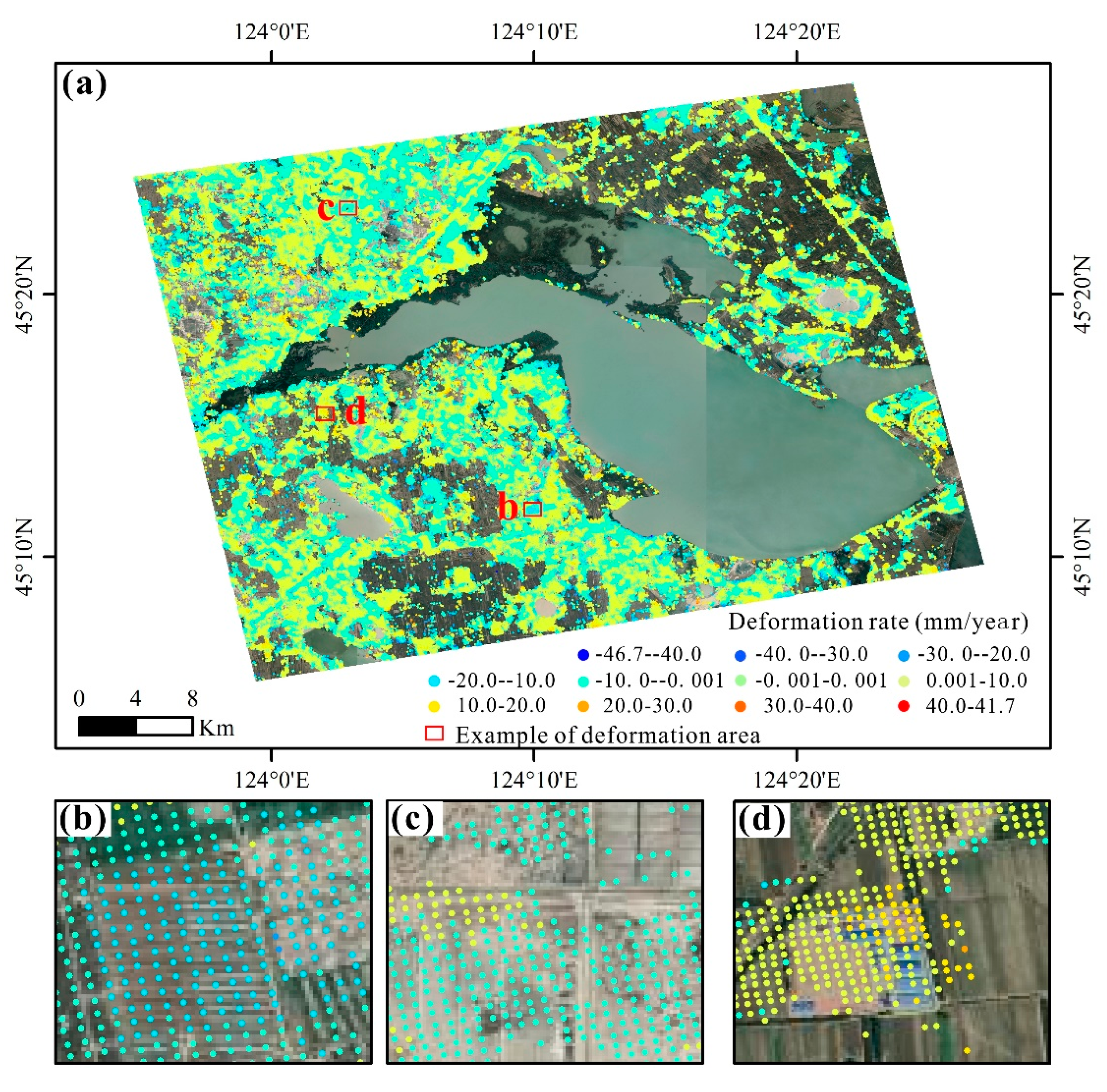
From the time-series deformation results in Figure 4, it can be seen that there were some time-series deformation areas in the Chagan Lake region. In order to further analyze the change in surface deformation with time in the study area, the land surface deformation rate of each temporarily coherent point (TCP) during the monitoring period was obtained from the time-series cumulative deformation results, as shown in Figure 5 and Table 3. The maximum subsidence rate and uplift rate in the study area were −46.7 mm/year and 41.7 mm/year, respectively.
As can be seen from Table 3, 367,691 temporarily coherent points were selected in the study area, of which 278,618 temporarily coherent points with an absolute annual deformation rate of less than 5 mm accounted for 76% of the total, and 349,081 temporarily coherent points with an absolute annual deformation rate of less than 10 mm accounted for 95% of the total. This shows that the land surface deformation in most areas of the study area was not large between December 2006 and December 2010.
3.2. Analysis of Land Surface Deformation Results
In order to study the differences in surface deformation between the three typical land types in the area (i.e., saline–alkali land, wetland, and highway), we used a Gaofen-2 (GF-2) image with a resolution of 0.8 m from the China Center for Resources Satellite Data and Application [41] to identify a saline–alkali area, a wetland area with dense vegetation cover, and two highways in the Chagan Lake region. Their specific locations in the study area are shown in Figure 1.
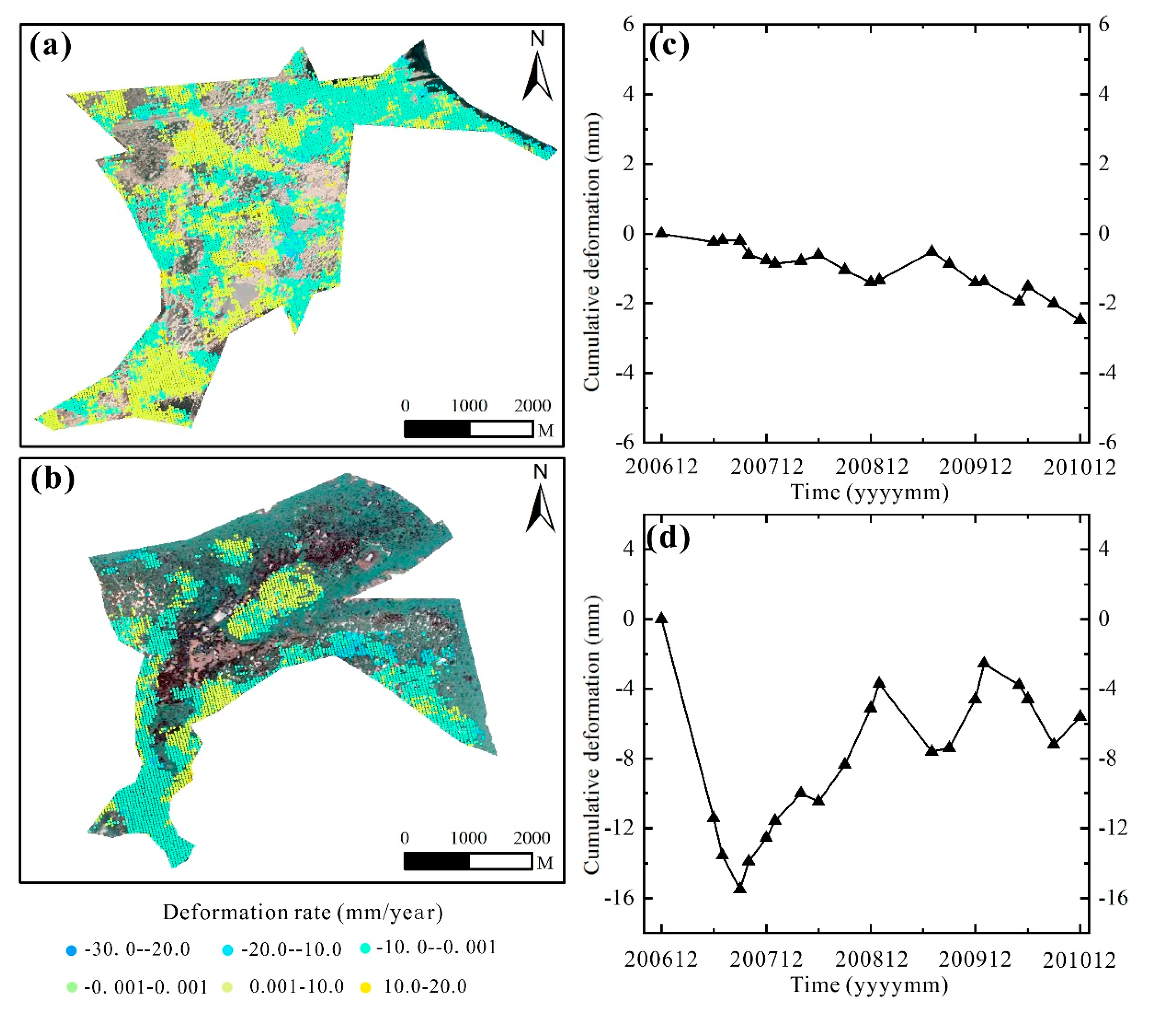
The deformation rate and the average cumulative time-series deformation of TCPs in the saline–alkali land and wetland areas were obtained by experiments, as shown in Figure 6. “Average cumulative time-series deformation” refers to the mean of the cumulative deformation of all TCPs in the area during the period from the first image’s acquisition to that image’s acquisition.
Figure 6 reflects the difference in deformation between the saline–alkali land and wetland areas in the study area. From Figure 6a,b, it can be seen that the positive and negative deformation rates in the saline–alkali area were roughly the same, while the deformation rate in the wetland area was predominantly negative, which indicated that most of the wetland area was in a subsidence state. Figure 6c,d shows that the average surface deformation of the saline–alkali land area and the wetland area was in a subsidence state between December 2006 and December 2010. The maximum subsidence of the wetland area was −15.5 mm in September 2007, and the final subsidence of the wetland area was larger than that of the saline–alkali area.
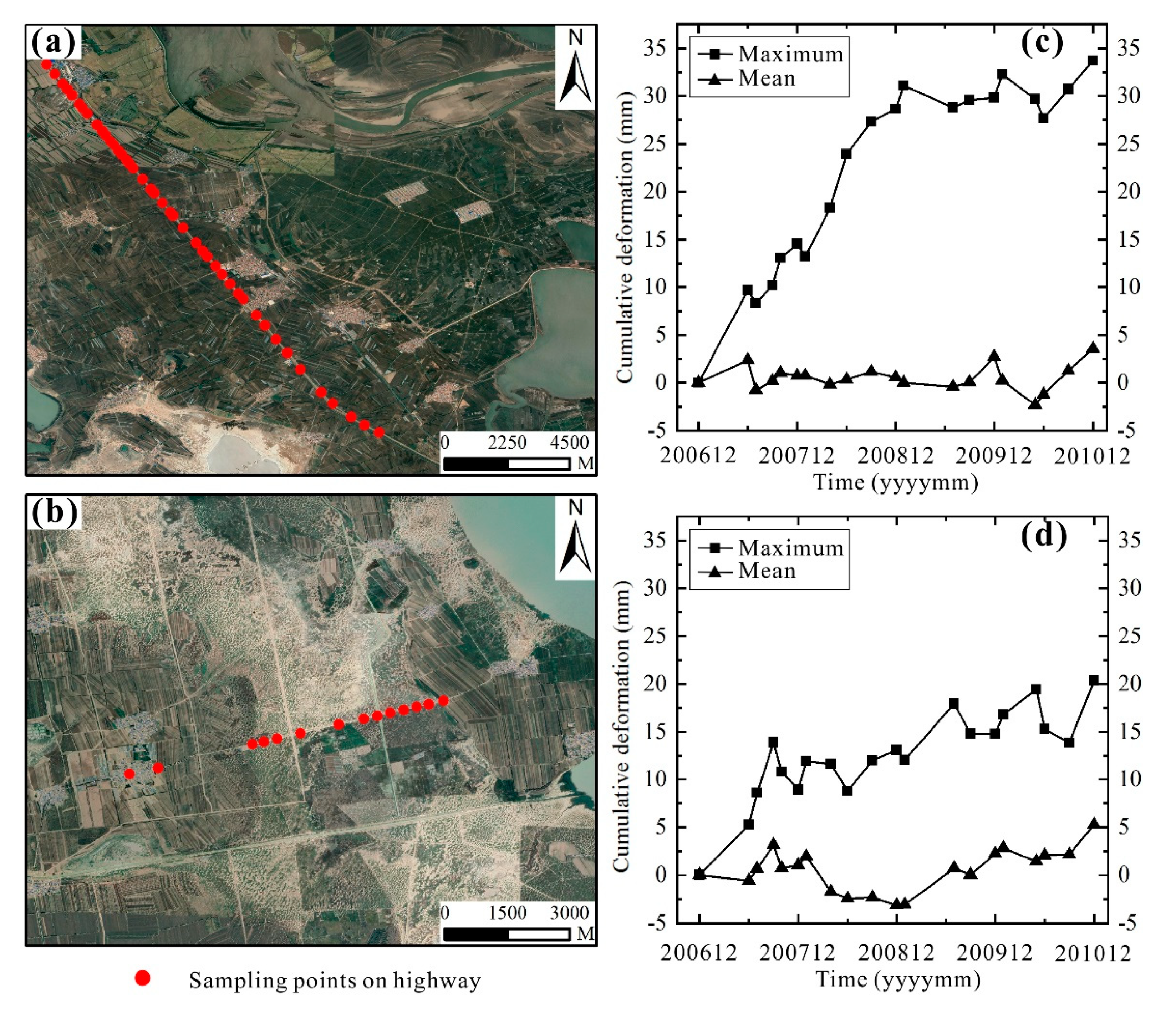
The surface deformation of two highways in different locations in the study area was analyzed, and the location and number of sampling points are shown in Figure 7a,b, respectively. Figure 7c,d shows the maximum and mean surface cumulative deformation of the sampling points on the two highways from December 2006 to December 2010, respectively. It can be seen that both Highway 1 and Highway 2 showed a certain uplift trend during the monitoring period. The maximum uplift of the sampling points was 33.7 mm and 20.4 mm for Highway 1 and Highway 2, respectively.
Taken together, Figure 1 and Figure 5 show that there were some differences in the land surface deformation rates between regions with and without dykes around Chagan Lake. In order to more accurately analyze the influence of concrete dykes on the surface deformation results, we separately selected sampling points in the area with dykes and without dykes near the lake, of which 40 points were selected in the area with dykes and 66 points were selected in the area without dykes. The specific locations of the selected points are shown in Figure 8.
The average deformation at the selected sampling points in the areas with and without dykes was calculated, and then the average cumulative time-series deformations of the different areas were obtained. The cumulative curves are shown in Figure 9.
Figure 9 shows that the land surface of the areas with or without dykes eventually presented a trend of subsidence from December 2006 to December 2010. The cumulative subsidence in the area with dykes was always smaller than that in the area without dykes, which shows that concrete dykes played a buffering role in land surface subsidence. The average time-series deformation in the areas with or without dykes showed a certain correlation with seasonal variation, i.e., the land surface tended to subside in spring and summer every year, while the land surface tended to rise in autumn and winter.
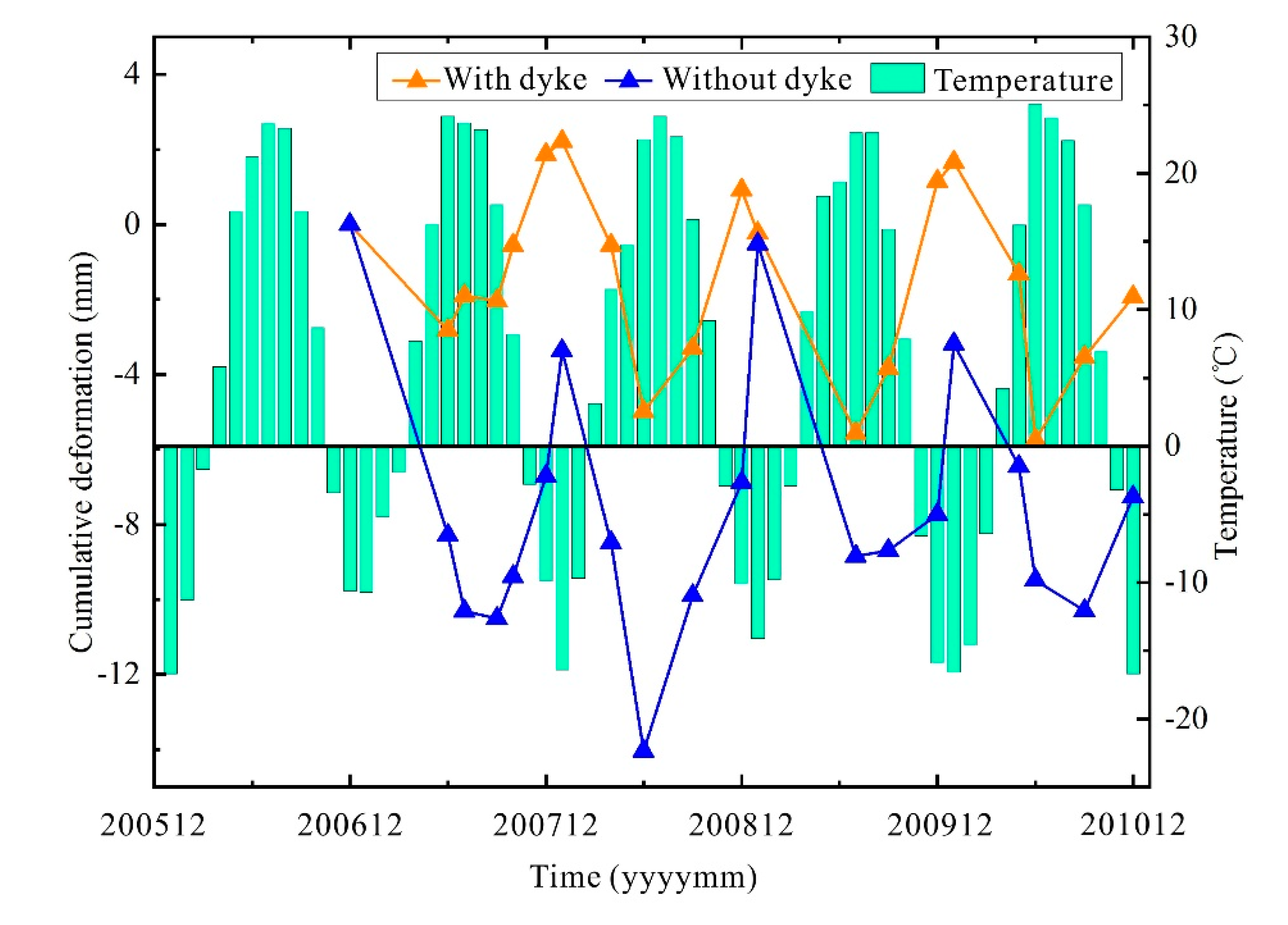
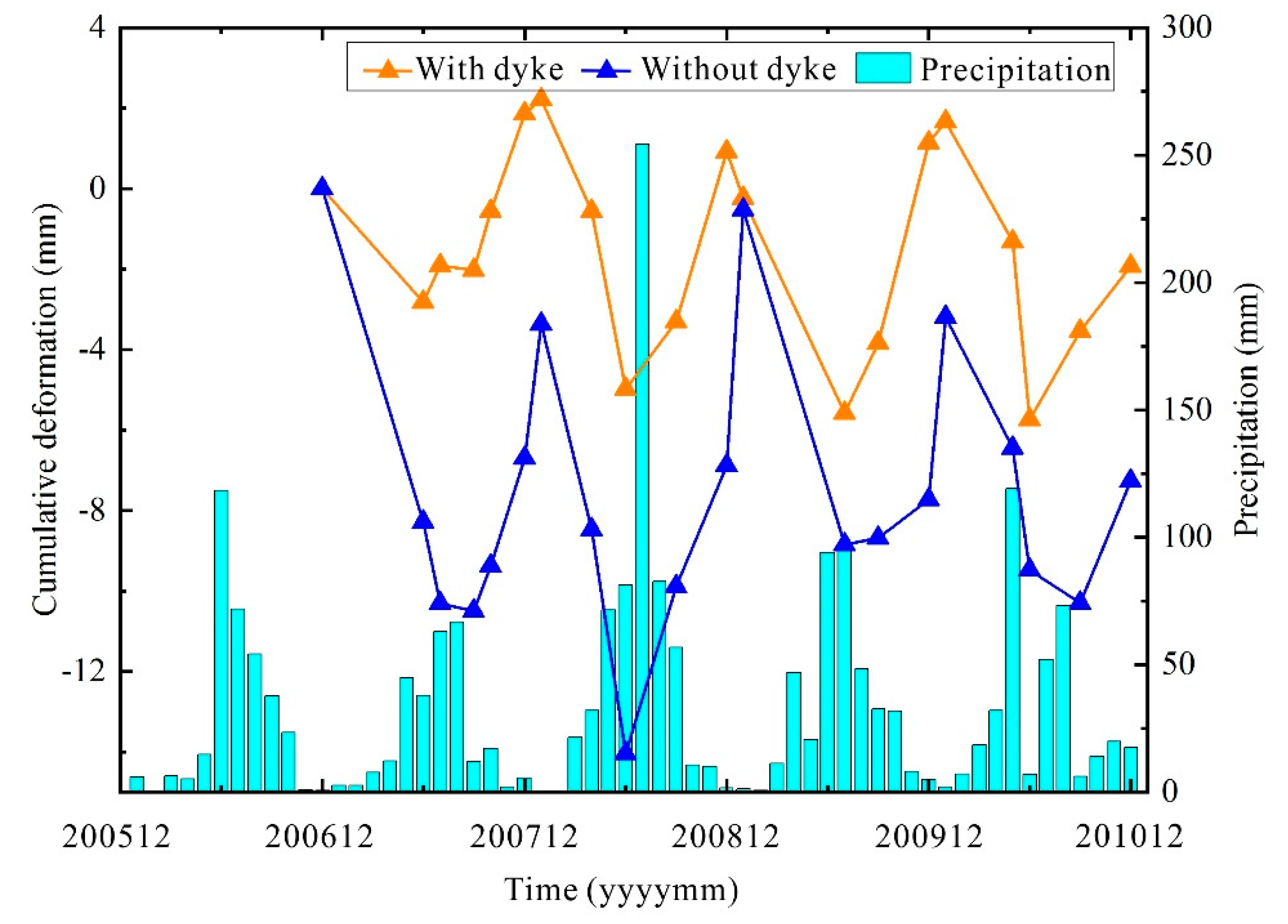
In order to verify the relationship between the seasonal variation and the land surface deformation trend in the lakeside areas with and without dykes, temperature and precipitation data for the period 2006 to 2010 from the meteorological station in Qianguoerros Mongolian Autonomous County, which is located approximately 30 km away from Chagan Lake, were obtained from the NOAA. We combined the temperature and precipitation data with the deformation information, and the results are shown in Figure 10 and Figure 11. The temperature value shown is the average temperature of each month, and the shown precipitation value is the sum of the precipitation in each month.
In Figure 10, it can be seen that there was a clear relationship between temperature and the monthly variation in the Chagan Lake region. The temperature rose from January to July and decreased from July to January. The warmest month of each year was July, when the temperature was approximately 25 °C, and the coldest month was January, when the temperature was approximately −15 °C.
As can be seen from Figure 10, the trend of the average time-series deformation of the areas with or without dykes near the lake was similar to the seasonal variation. As the temperature rose, the land surface showed a subsidence trend, and the land surface showed an upward trend as the temperature decreased. This phenomenon was mainly caused by seasonal frozen soil in the Chagan Lake region. As the temperature decreased, soil freezing led to volume expansion, which raised the land surface. As the temperature increased, the frozen soil gradually melted, and the volume shrank, resulting in land surface subsidence [42,43].
It can be seen from Figure 11 that the monthly total precipitation in the study area changed significantly with the month. Compared to other seasons, there was more precipitation in summer. Land surface deformation and precipitation showed a certain degree of negative correlation with the change in month, i.e., in months with more precipitation, surface subsidence appeared. This was because the demand for irrigation for cash crops, such as in farmland and orchards, is large in summer, which leads to a large amount of groundwater being exploited [44,45]. Although there is a large amount of precipitation in summer, it takes a certain amount of time to convert the precipitation into groundwater, i.e., there is latency between precipitation and groundwater recharge, and the groundwater level remains in a declining state. Therefore, the surface of the lakeside areas with or without dykes was in a state of subsidence. In winter, although there is less precipitation, agriculture is in a fallow period at the same time, i.e., there is less exploitation of groundwater and the groundwater level is increased by precipitation, so the land surface of the lakeside areas with or without dykes was in a rising state.
Table 4 shows the relationship between the average cumulative time-series deformation of the lakeside areas with or without dykes and the corresponding monthly meteorological data in different time series.
In order to further quantitatively analyze the relationship between the average cumulative time-series deformation and the meteorological data, we studied the correlations between the average cumulative time-series deformation and the monthly mean temperature and monthly total precipitation in the lakeside areas with or without dykes at different times, obtaining linear fitting equations and correlation coefficients (R), as shown in Figure 12.
From Figure 12, it can be seen that the average cumulative time-series deformation in the lakeside areas with or without dykes was negatively correlated with the monthly average temperature, and the correlation coefficients (R) were −0.822 and −0.734, respectively. The average cumulative time-series deformation of the lakeside areas with or without dykes also showed a negative correlation with the monthly total precipitation, and the correlation coefficients (R) were −0.513 and −0.431, respectively. Compared to precipitation, the correlation between average cumulative time-series deformation and monthly mean temperature was higher.
4. Discussion
In this study, the Chagan Lake region was taken as a study area. Using ALOS PALSAR images with strong penetration and the TCPInSAR method, the deformation rate and the time-series cumulative deformation in the study area from December 2006 to December 2010 were obtained.
During the monitoring period, the surface deformation rate in the study area was not large on the whole; however, the deformation in different areas was different. In this study, saline–alkali land, wetland, and two highways were selected as representative land types. Through experiments, it was found that both the saline–alkali land area and the wetland area were in a state of subsidence during the monitoring period, while the land surface of the highway areas slightly rose, which shows that the highways could buffer land surface subsidence to a certain extent. Further, by comparing the difference in subsidence of the lakeside areas with or without dykes, it was found that the subsidence of the area with dykes was smaller than that of the area without dykes, which proved once again that artificial structures could restrain surface subsidence.
On the basis of an analysis of the relationship between lakeside land surface deformation and meteorological data, it was found that both temperature and precipitation had a negative correlation with surface deformation. Using this phenomenon, we further analyzed the effect of soil freezing and thawing on surface deformation and explained that the variation trend of surface deformation with groundwater circulation was affected by precipitation and groundwater overexploitation.
Monitoring and analyzing the surface deformation in the Chagan Lake region can (i) provide a data reference for saline–alkali land improvement projects [46], environmental protection in wetlands, ecological and geological environment improvement projects, and earthquake monitoring and prediction in mining areas of Songyuan City; (ii) improve the degree of monitoring and control of disasters caused by surface deformation; and (iii) lay a foundation for sustainable ecological and economic development.
5. Conclusions
In this study, surface deformation in the Chagan Lake region in Songyuan City from 2006 to 2010 was determined, and the deformation in areas with three typical types of land cover was compared. Combining meteorological data and taking lakeside areas as an example, we analyzed the factors that had an influence on surface deformation. Our conclusions are as follows:
- During the monitoring period, the maximum land surface subsidence rate and the maximum uplift rate in the Chagan Lake region were −46.7 mm/year and 41.7 mm/year, respectively. There were 278,618 temporarily coherent points in the study area whose absolute annual average deformation rate value was less than 5 mm, accounting for 76% of the total, and 349,081 points whose absolute value was less than 10 mm, accounting for 95% of the total, which shows that most of the study area experienced little deformation during the monitoring period;
- Through an analysis of the deformation of a wetland area with dense vegetation cover, a saline–alkali land area without vegetation cover, and two highways in the study area, it was found that both the wetland area and the saline–alkali land area experienced a certain degree of subsidence, but the subsidence of the saline–alkali area was far less than that of the wetland area, and the surface of the highways remained relatively stable during the monitoring period, showing a slight upward trend. In addition, by selecting sampling points to observe the time-series deformation, it was found that the lakeside area was in a state of subsidence during the monitoring period. Compared to the lakeside area without dykes, the average time-series subsidence of the lakeside area with concrete dykes was smaller, which indicated that the concrete dykes had a certain buffering effect on the lakeside land surface’s subsidence;
- Using meteorological data and analyzing surface deformation in the lakeside areas, we found that surface deformation was negatively correlated with temperature and precipitation to a certain extent. In winter, agriculture is in a fallow period, the groundwater is supplemented by precipitation, the groundwater level rises, and the decrease in temperature causes soil frost heaving, so the land surface was in a state of uplift. In summer, the demand for irrigation for agriculture is high, there is latency between precipitation and groundwater recharge, the groundwater level decreases, and the increase in temperature leads to the thawing of frozen soil, so the land surface was in a state of subsidence;
- Using the TCPInSAR method (which does not require phase unwrapping and can effectively mitigate the orbital error and atmospheric phase delay) and L-band ALOS PALSAR images with strong penetration, we could obtain time-series surface deformation results in the study area quickly. By analyzing the difference in surface deformation in areas with three typical types of land cover and the negative correlation between surface deformation in lakeside areas and meteorological data, we have helped provide a basis for making decisions on sustainable development issues, such as in economic development, urban planning, and geological disaster prevention, in the Chagan Lake region.
Author Contributions
Conceptualization, F.W. and Q.D.; software, L.Z.; validation, Q.W. and L.Z.; data curation, M.W.; writing—original draft preparation, F.W.; writing—review and editing, Q.D.; funding acquisition, F.W., Q.W., and M.W.
Funding
This work was supported by the National Natural Science Foundation of China (Grant Nos. 41472243 and 41820104001); the Open Fund of Key Laboratory of Land Subsidence Monitoring and Prevention, Ministry of Land and Resources of China (Grant No. KLLSMP201901); and the Open Fund of Key Laboratory of Urban Land Resources Monitoring and Simulation, Ministry of Land and Resources of China (Grant No. KF-2018-03-020).
Acknowledgments
The ALOS PALSAR data were provided by the National Space Development Agency (NASDA) of Japan, the SRTM DEM data were provided by the United States Geological Survey (USGS), the GF-2 image was provided by the China Centre for Resources Satellite Data and Application, and the temperature and precipitation data were provided by the National Oceanic and Atmospheric Administration (NOAA). We are grateful for this support.
Conflicts of Interest
The authors declare no conflicts of interest.
References
- Peltier, A.; Scott, B.; Hurst, T. Ground deformation patterns at White Island volcano (New Zealand) between 1967 and 2008 deduced from levelling data. J. Volcanol. Geotherm. Res. 2009, 181, 207–218. [Google Scholar] [CrossRef]
- Palano, M.; Guarrera, E.; Mattia, M. GPS ground deformation patterns at Mount St. Helens (Washington, DC, USA) from 2004 to 2010. Terra Nova 2012, 24, 148–155. [Google Scholar] [CrossRef]
- Qi, B.; Niu, W.M. A technological study of the monitoring system for layerwise mark in the Tianjin Binhai New Area. Hydrogeol. Eng. Geol. 2011, 38, 44–48. [Google Scholar]
- Ferretti, A.; Savio, G.; Barzaghi, R.; Borghi, A.; Musazzi, S.; Novali, F.; Prati, C.; Rocca, F. Submillimeter accuracy of InSAR time series: Experimental validation. IEEE Trans. Geosci. Remote Sens. 2007, 45, 1142–1153. [Google Scholar] [CrossRef]
- Aimaiti, Y.; Yamazaki, F.; Liu, W. Multi-Sensor InSAR analysis of progressive land subsidence over the coastal city of Urayasu, Japan. Remote Sens. 2018, 10, 1034. [Google Scholar] [CrossRef]
- Lu, Z.; Masterlark, T.; Dzurisin, D. Interferometric synthetic aperture radar study of Okmok volcano, Alaska, 1992–2003: Magma supply dynamics and postemplacement lava flow deformation. J. Geophys. Res. Solid Earth 2005, 110, B02403-n/a. [Google Scholar] [CrossRef]
- Sun, Q.; Zhang, L.; Ding, X.L.; Hu, J.; Liang, H.Y. Investigation of Slow-Moving Landslides from ALOS/PALSAR Images with TCPInSAR: A Case Study of Oso, USA. Remote Sens. 2015, 7, 72–88. [Google Scholar] [CrossRef]
- Rossi, M.; Peltzer, G.; Adragna, F.; Carmona, C.; Massonnet, D.; Feigl, K.; Rabaute, T. The displacement field of the Landers earthquake mapped by radar interferometry. Nature 1993, 364, 138–142. [Google Scholar]
- Zhou, W.; Chen, F.L.; Guo, H.D. Differential radar interferometry for structural and ground deformation monitoring: A new tool for the conservation and sustainability of cultural heritage sites. Sustainability 2015, 7, 1712–1729. [Google Scholar] [CrossRef]
- Chu, T.; Lindenschmidt, K. Comparison and validation of digital elevation models derived from InSAR for a flat inland Delta in the high latitudes of Northern Canada. Can. J. Remote Sens. 2017, 43, 109–123. [Google Scholar] [CrossRef]
- Fruneau, B.; Achache, J.; Delacourt, C. Observation and modelling of the Saint-Étienne-de-Tinée landslide using SAR interferometry. Tectonophysics 1996, 265, 181–190. [Google Scholar] [CrossRef]
- Liu, G.X. Monitoring of Ground Deformations with Radar Interferometry; SinoMaps Press: Beijing, China, 2005; pp. 58–70. [Google Scholar]
- Colesanti, C.; Wasowski, J. Investigating landslides with space-borne synthetic aperture radar (SAR) interferometry. Eng. Geol. 2006, 88, 173–199. [Google Scholar] [CrossRef]
- Zhao, Q.; Yang, G.D.; Zhang, X.Q.; Shao, P. Inversion analysis of co-seismic deformation field of Jiuzhaigou earthquake based on D-InSAR. Glob. Geol. 2018, 37, 938–944. [Google Scholar]
- Ferretti, A.; Prati, C.; Rocca, F. Nonlinear subsidence rate estimation using permanent scatterers in differential SAR interferometry. IEEE Trans. Geosci. Remote Sens. 2000, 38, 2202–2212. [Google Scholar] [CrossRef] [Green Version]
- Chen, G.; Zhang, Y.; Zeng, R.Q.; Yang, Z.K.; Chen, X.; Zhao, F.M.; Meng, X.M. Detection of land subsidence associated with land creation and rapid urbanization in the Chinese Loess Plateau using time series InSAR: A case study of Lanzhou New District. Remote Sens. 2018, 10, 270. [Google Scholar] [CrossRef]
- Berardino, P.; Fornaro, G.; Lanari, R.; Sansosti, E. A new algorithm for surface deformation monitoring based on small baseline differential SAR interferograms. IEEE Trans. Geosci. Remote Sens. 2002, 40, 2375–2383. [Google Scholar] [CrossRef] [Green Version]
- Wang, Y.Y.; Guo, Y.H.; Hu, S.Q.; Li, Y.; Wang, J.Z.; Liu, X.S.; Wang, L. Ground deformation analysis using InSAR and backpropagation prediction with influencing factors in Erhai Region, China. Sustainability 2019, 11, 2853. [Google Scholar] [CrossRef]
- Polcari, M.; Albano, M.; Montuori, A.; Bignami, C.; Tolomei, C.; Pezzo, G.; Falcone, S.; La Piana, C.; Doumaz, F.; Salvi, S.; et al. InSAR monitoring of Italian coastline revealing natural and anthropogenic ground deformation phenomena and future perspectives. Sustainability 2018, 10, 3152. [Google Scholar] [CrossRef]
- Li, N.; Wu, J. Research on methods of high coherent target extraction in urban area based on Psinsar technology. Int. Arch. Photogramm. Remote Sens. Spat. Inf. Sci. 2018, 42, 901–908. [Google Scholar] [CrossRef]
- Zhou, L.; Guo, J.M.; Hu, J.Y.; Li, J.W.; Xu, Y.F.; Pan, Y.J.; Shi, M. Wuhan surface subsidence analysis in 2015–2016 based on Sentinel-1A data by SBAS-InSAR. Remote Sens. 2017, 9, 982. [Google Scholar] [CrossRef]
- Vajedian, S.; Motagh, M.; Nilfouroushan, F. StaMPS Improvement for deformation analysis in mountainous regions: Implications for the Damavand Volcano and Mosha Fault in Alborz. Remote Sens. 2015, 7, 8323–8347. [Google Scholar] [CrossRef]
- Zhang, L.; Lu, Z.; Ding, X.L.; Jung, H.S.; Feng, G.C.; Lee, C.W. Mapping ground surface deformation using temporarily coherent point SAR interferometry: Application to Los Angeles Basin. Remote Sens. Environ. 2012, 117, 429–439. [Google Scholar] [CrossRef]
- Cho, M.; Zhang, L.; Lee, C.W. Monitoring of Volcanic activity of Augustine Volcano, Alaska using TCPInSAR and SBAS time-series techniques for measuring surface deformation. Korean J. Remote Sens. 2013, 29. [Google Scholar] [CrossRef]
- Liu, G.; Jia, H.; Nie, Y.; Li, T.; Zhang, R.; Yu, B.; Li, Z. Detecting subsidence in coastal areas by ultrashort-baseline TCPInSAR on the time series of high-resolution TerraSAR-X images. IEEE Trans. Geosci. Remote Sens. 2014, 52, 1911–1923. [Google Scholar]
- Sun, G.Y.; Tian, W.; Jia, Z.G.; Wang, H.X.; Ma, G.Q.; Bi, S.X.; Xu, N.; Wang, J.H.; Yao, Y.L. Risk analysis and mitigation on the impact of the development of Songyuan irrigation area on the ecology of Lake Chagan. J. Lake Sci. 2014, 26, 66–73. [Google Scholar]
- Cheng, P. Research of the Influence from the Development of Songyuan Irrigation Area to Soil Salinization. Master’s Thesis, Jilin University, Changchun, China, 2016. [Google Scholar]
- Wang, S.J.; Chen, Z.G.; Qin, W.J.; Liu, Y.; Liu, F.; Gan, J. Using DInSAR to monitor frost heaving and Thaw settlement deformation of highway subgrade in seasonal frozen soil zone. J. Wuhan Univ. Technol. 2018, 42, 58–62. [Google Scholar]
- Sun, S.; Zhang, G.X.; Huang, Z.G.; Xu, C.; Li, R.R. Hydrological regimes of Chagan lake in Western Jilin province. Wetl. Sci. 2014, 12, 43–48. [Google Scholar]
- Santoro, M.; Fransson, J.E.S.; Eriksson, L.E.B.; Magnusson, M.; Ulander, L.M.H.; Olsson, H. Signatures of ALOS PALSAR L-Band Backscatter in Swedish Forest. IEEE Trans. Geosci. Remote Sens. 2009, 47, 4001–4019. [Google Scholar] [CrossRef] [Green Version]
- Land Processes Distributed Active Archive Center Web Page. Available online: http://gdex.cr.usgs.gov/gdex/ (accessed on 10 June 2019).
- National Centers for Environmental Information Web Page. Available online: https://gis.ncdc.noaa.gov/maps/ncei/summaries/monthly (accessed on 6 July 2019).
- Zhang, L.; Ding, X.L.; Lu, Z. Ground settlement monitoring based on temporarily coherent points between two SAR acquisitions. ISPRS J. Photogramm. Remote Sens. 2011, 66, 146–152. [Google Scholar] [CrossRef]
- Zhang, L.; Ding, X.L.; Lu, Z. Modeling PSInSAR time series without phase unwrapping. IEEE Trans. Geosci. Remote Sens. 2011, 49, 547–556. [Google Scholar] [CrossRef]
- Zhang, L.; Ding, X.L.; Lu, Z.; Jung, H.; Hu, J.; Feng, G. A novel multitemporal InSAR model for joint estimation of deformation rates and orbital errors. IEEE Trans. Geosci. Remote Sens. 2014, 52, 3529–3540. [Google Scholar] [CrossRef]
- Jia, J.H.; Huang, M.; Liu, X.L. Surface reconstruction algorithm based on 3D Delaunay Triangulation. Acta Geod. Cartogr. Sin. 2018, 47, 281–290. [Google Scholar]
- Bamler, R. Interferometric stereo radargrammetry: Absolute height determination from ERS-ENVISAT interferograms. IEEE Proc. IGARSS 2000, 2, 742–745. [Google Scholar]
- Jiao, M.L.; Jiang, T.C. Synthetic Aperture Radar Interferometry Theory and Application; SinoMaps Press: Beijing, China, 2009; pp. 39–41. [Google Scholar]
- Jiang, M.; Ding, X.L.; Li, Z.W.; Tian, X.; Wang, C.S.; Zhu, W. InSAR coherence estimation for small data sets and its impact on temporal decorrelation extraction. IEEE Trans. Geosci. Remote Sens. 2014, 52, 6584–6596. [Google Scholar] [CrossRef]
- Lin, Y.N.; Simons, M.; Hetland, E.A.; Muse, P.; DiCaprio, C. A multiscale approach to estimating topographically correlated propagation delays in radar interferograms. Geochem. Geophys. Geosyst. 2010, 11. [Google Scholar] [CrossRef]
- China Centre for Resources Satellite Data and Application Home Page. Available online: http://www.cresda.com/CN/ (accessed on 14 June 2019).
- Chen, Y.X.; Jiang, L.M.; Liang, L.L.; Zhou, Z.W. Monitoring permaforst deformation in the upstream Heihe River, Qilian Mountain by using multi-temporal Sentinel InSAR dataset. Chin. J. Geophys. 2019, 62, 2441–2454. [Google Scholar]
- Li, S.S.; Li, Z.W.; Hu, J.; Sun, Q.; Yu, X.Y. Investigation of the Seasonal oscillation of the permaforst over Qinghai-Tibet Plateau with SBAS-InSAR algorithm. Chin. J. Geophys. 2013, 56, 1476–1486. [Google Scholar]
- Motagh, M.; Walter, T.R.; Sharifi, M.A.; Fielding, E.; Schenk, A.; Anderssohn, J.; Zschau, J. Land subsidence in Iran caused by widespread water reservoir overexploitation. Geophys. Res. Lett. 2008, 35, L16403. [Google Scholar] [CrossRef]
- Motagh, M.; Shamshiri, R.; Haghighi, M.H.; Wetzel, H.U.; Akbari, B.; Nahavandchi, H.; Roessner, S.; Arabi, S. Quantifying groundwater exploitation induced subsidence in the Rafsanjan plain, southeastern Iran, using InSAR time-series and in situ measurements. Eng. Geol. 2017, 218, 134–151. [Google Scholar] [CrossRef]
- Liu, L.; Bai, X.; Jiang, Z. The generic technology identification of saline–alkali land management and improvement based on social network analysis. Clust. Comput. 2018, 1–10. [Google Scholar] [CrossRef]
Figure 1.
The location of (and basic information on) the study area.

Figure 2.
The data processing flow of the temporarily coherent point synthetic aperture radar interferometry (TCPInSAR) method.
Figure 2.
The data processing flow of the temporarily coherent point synthetic aperture radar interferometry (TCPInSAR) method.

Figure 3.
The time baseline and spatial baseline of interference pairs. Each green dot represents an ALOS PALSAR image, and each blue line represents the connection of an interference pair.
Figure 3.
The time baseline and spatial baseline of interference pairs. Each green dot represents an ALOS PALSAR image, and each blue line represents the connection of an interference pair.

Figure 4.
The time-series cumulative deformation results for the study area.

Figure 5.
(a) The land surface deformation rate in the study area; (b) an example of a land surface subsidence area; (c) an example of an area with less land surface deformation; (d) an example of an area with surface uplift.
Figure 5.
(a) The land surface deformation rate in the study area; (b) an example of a land surface subsidence area; (c) an example of an area with less land surface deformation; (d) an example of an area with surface uplift.

Figure 6.
Differences in surface deformation between saline–alkali land and wetland areas. (a) The surface deformation rate in the saline–alkali area; (b) the surface deformation rate in the wetland area; (c) the average time-series deformation of temporarily coherent points (TCPs) in the saline–alkali area; (d) the average time-series deformation of TCPs in the wetland area.

Figure 7.
Differences in surface deformation between two highways. (a) The position distribution of Highway 1’s deformation sampling points; (b) the position distribution of Highway 2’s deformation sampling points; (c) the maximum and mean time-series deformation of Highway 1’s sampling points; (d) the maximum and mean time-series deformation of Highway 2’s sampling points.

Figure 8.
(a) The position distribution of deformation sampling points in the lakeside area with or without dykes; (b) a Gaofen-2 (GF-2) image of the lakeside area with dykes; (c) a GF-2 image of the lakeside area without dykes.
Figure 8.
(a) The position distribution of deformation sampling points in the lakeside area with or without dykes; (b) a Gaofen-2 (GF-2) image of the lakeside area with dykes; (c) a GF-2 image of the lakeside area without dykes.

Figure 9.
The average time-series deformation in the areas with and without dykes.

Figure 10.
The relationship between the average time-series deformation and the monthly mean temperature.
Figure 10.
The relationship between the average time-series deformation and the monthly mean temperature.

Figure 11.
The relationship between the average time-series deformation and the monthly total precipitation.
Figure 11.
The relationship between the average time-series deformation and the monthly total precipitation.

Figure 12.
(a) Correlations between average time-series cumulative deformation and monthly mean temperature; (b) correlations between average time-series cumulative deformation and monthly total precipitation.
Figure 12.
(a) Correlations between average time-series cumulative deformation and monthly mean temperature; (b) correlations between average time-series cumulative deformation and monthly total precipitation.


Table 1.
The specific parameters of the ALOS PALSAR images that were selected for the experiment. FBS: fine-beam single polarization; FBD: fine-beam dual polarization.
Table 1.
The specific parameters of the ALOS PALSAR images that were selected for the experiment. FBS: fine-beam single polarization; FBD: fine-beam dual polarization.
| Image Number | Imaging Time (yyyymmdd) | Imaging Mode | Image Number | Imaging Time (yyyymmdd) | Imaging Mode |
|---|---|---|---|---|---|
| 1 | 20061206 | FBS | 11 | 20081211 | FBS |
| 2 | 20070608 | FBD | 12 | 20090126 | FBS |
| 3 | 20070724 | FBD | 13 | 20090729 | FBD |
| 4 | 20070908 | FBD | 14 | 20090913 | FBD |
| 5 | 20071024 | FBS | 15 | 20091214 | FBS |
| 6 | 20071209 | FBS | 16 | 20100129 | FBS |
| 7 | 20080124 | FBS | 17 | 20100501 | FBD |
| 8 | 20080425 | FBD | 18 | 20100616 | FBD |
| 9 | 20080610 | FBD | 19 | 20100916 | FBD |
| 10 | 20080910 | FBD | 20 | 20101217 | FBS |
Table 2.
Temperature and precipitation data for the study area from 2006 to 2010.
| Number | Time (yyyymm) | Temperature (°C) | Precipitation (mm) |
|---|---|---|---|
| 1 | 200601 | −16.7 | 5.84 |
| 2 | 200602 | −11.3 | 0.00 |
| 3 | 200603 | −1.7 | 6.35 |
| 4 | 200604 | 5.8 | 5.08 |
| 5 | 200605 | 17.2 | 14.73 |
| 6 | 200606 | 21.2 | 118.36 |
| 58 | 201010 | 7.0 | 13.97 |
| 59 | 201011 | −3.2 | 19.81 |
| 60 | 201012 | −16.7 | 17.53 |
Table 3.
Statistics of the deformation rate. TCP: temporarily coherent point.
| Deformation Rate (mm/year) | Number of TCPs | Percentage of Total TCPs (%) |
|---|---|---|
| −5–5 | 278,618 | 76 |
| −10–10 | 349,081 | 95 |
| −46.7–41.7 | 367,691 | 100 |
Table 4.
The relationship between the average cumulative time-series deformation in the lakeside areas with or without dykes and meteorological data.
Table 4.
The relationship between the average cumulative time-series deformation in the lakeside areas with or without dykes and meteorological data.
| Image Acquisition Date (yyymmdd) | Deformation of the Area with Dykes (mm) | Deformation of the Area without Dykes (mm) | Meteorological Data Acquisition Date (yyyymm) | Temperature (°C) | Precipitation (mm) |
| 20061206 | 0 | 0 | 200612 | −10.6 | 0.51 |
| 20070608 | −2.8 | −8.3 | 200706 | 24.2 | 37.85 |
| 20070724 | −1.9 | −10.3 | 200707 | 23.7 | 62.99 |
| 20070908 | −2.0 | −10.5 | 200709 | 17.7 | 11.94 |
| 20071024 | −0.6 | −9.4 | 200710 | 8.2 | 17.02 |
| 20071209 | 1.9 | −6.7 | 200712 | −9.9 | 5.59 |
| 20080124 | 2.2 | −3.4 | 200801 | −16.4 | 0.00 |
| 20080425 | −0.6 | −8.5 | 200804 | 11.5 | 32.00 |
| 20080610 | −5.0 | −14.0 | 200806 | 22.5 | 81.28 |
| 20080910 | −3.3 | −9.9 | 200809 | 16.6 | 56.64 |
| 20081211 | 0.9 | −6.9 | 200812 | −10.0 | 1.52 |
| 20090126 | −0.2 | −0.5 | 200901 | −14.0 | 1.27 |
| 20090729 | −5.6 | −8.8 | 200907 | 23 | 94.49 |
| 20090913 | −3.8 | −8.7 | 200909 | 15.9 | 32.51 |
| 20091214 | 1.1 | −7.7 | 200912 | −15.9 | 4.83 |
| 20100129 | 1.6 | −3.2 | 201001 | −16.6 | 2.03 |
| 20100501 | −1.3 | −6.4 | 201005 | 16.2 | 119.13 |
| 20100616 | −5.7 | −9.5 | 201006 | 25.1 | 6.86 |
| 20100916 | −3.5 | −10.3 | 201009 | 17.7 | 6.10 |
| 20101217 | −1.9 | −7.3 | 201012 | −16.7 | 17.53 |
© 2019 by the authors. Licensee MDPI, Basel, Switzerland. This article is an open access article distributed under the terms and conditions of the Creative Commons Attribution (CC BY) license (http://creativecommons.org/licenses/by/4.0/).
Share and Cite
MDPI and ACS Style
Wang, F.; Ding, Q.; Zhang, L.; Wang, M.; Wang, Q. Analysis of Land Surface Deformation in Chagan Lake Region Using TCPInSAR. Sustainability 2019, 11, 5090. https://0-doi-org.brum.beds.ac.uk/10.3390/su11185090
AMA Style
Wang F, Ding Q, Zhang L, Wang M, Wang Q. Analysis of Land Surface Deformation in Chagan Lake Region Using TCPInSAR. Sustainability. 2019; 11(18):5090. https://0-doi-org.brum.beds.ac.uk/10.3390/su11185090
Chicago/Turabian StyleWang, Fengyan, Qing Ding, Lei Zhang, Mingchang Wang, and Qing Wang. 2019. "Analysis of Land Surface Deformation in Chagan Lake Region Using TCPInSAR" Sustainability 11, no. 18: 5090. https://0-doi-org.brum.beds.ac.uk/10.3390/su11185090
Note that from the first issue of 2016, this journal uses article numbers instead of page numbers. See further details here.