Intra- and Inter-Annual Variability of Hydrometeorological Variables in the Jinsha River Basin, Southwest China

1
College of Automation, Huaiyin Institute of Technology, Huaian 223003, China
2
School of Hydropower and Information Engineering, Huazhong University of Science and Technology, Wuhan 430074, China
*
Author to whom correspondence should be addressed.
Sustainability 2019, 11(19), 5142; https://0-doi-org.brum.beds.ac.uk/10.3390/su11195142
Submission received: 21 July 2019
/
Revised: 10 September 2019
/
Accepted: 17 September 2019
/
Published: 20 September 2019
(This article belongs to the Special Issue Uncertainty of Climate Change Impacts on Hydrology, Water Quality and Ecology)
Abstract
:In this study, the intra- and inter-annual variability of three major elements in the water system, temperature, precipitation and streamflow, from 1974 to 2010 in the Jinsha River Basin, China, were analyzed. An exploratory data analysis method, namely, moving average over shifting horizon (MASH), was introduced and combined with the Mann–Kendall (MK) test and Sen’s slope estimation to analyze the intra- and inter-annual variations. The combination of MASH with the MK test and Sen’s slope estimation demonstrated that the annual temperature, precipitation and streamflow from 1974 to 2010 showed, on average, an increasing trend. The highest change in temperature was detected in early January, 0.8 ℃, that of precipitation was detected in late June, 0.4 mm/day, and that of streamflow was detected mid-August, 138 mm/day. Sensitivity analysis of the smoothing parameters on estimated trends demonstrated that Y parameters smaller than 2 and w parameters smaller than 6 were not suitable for trend detection when applying the MASH method. The correlation between the smoothed data was generally greater than that between the original hydrometeorological data, which demonstrated that the application of MASH could eliminate the influence of periodicity and random fluctuations on hydrometeorological time series and could facilitate regularity and the detection of trends.
1. Introduction
It has always been important to explore the temporal and spatial distribution of hydrometeorological variables in the nonlinear dynamic water-cycle system [1,2,3]. Affected by global warming and human activities, the trend and periodicity of precipitation and streamflow processes have experienced strong changes [4]. The frequency and intensity of extreme hydrometeorological events such as floods, droughts and urban rainstorms have increased significantly [5]. Regional water shortages have become heavier, which has had a crippling effect on the development of human society and economy [6,7].
Hydrometeorological variables like temperature, precipitation and streamflow are three major elements in the natural water cycle. Their changes can affect the formation, development and evolution of water resources. It is of great importance to research the temporal and spatial variations of hydrometeorological variables for the efficient allocation and sustainable utilization of water resources. Stocker et al. [8], Xu et al. [9], Feng et al. [10] and Nilsson et al. [11] have researched the trends of different hydro-climatic variables in China. The IPCC reported in its fifth assessment report in 2014 that the surface temperature in China had risen by 0.9 ℃ since 1913 [8]. As for the precipitation, the changing amount of precipitation was low from the 1950s to the 1970s, but the rainfall belt gradually shifted from North China to South China and the Yangtze River Basin. Since the 21st century the rainfall belt has moved back in the northward direction [8]. The drastic change in the spatial and temporal distribution of temperature and precipitation has led to changes in the streamflow in the basin [9]. Streamflow in many areas of China has shown a decreasing trend, especially in the Hai River Basin and the Yellow River Basin in recent decades [10]. In addition to temperature and rainfall, fragmentation of the natural runoff system has been a severe effect of water engineering projects. Nilsson et al. [11] pointed out in his research in 2013 that about 59% of the streamflow processes for the river systems all over the world have changed significantly due to dam construction.
Under the strong influence of global warming and human activities, the hydrometeorological process changed substantially, which aggravated the uneven spatial and temporal distribution of water resources in China and increased the frequency, scope and impact of natural disasters such as drought and flood. Therefore, it is of great importance to conduct in-depth analyses of the trends of hydrometeorological variables in a watershed. Generally, trend detection methods for hydrometeorological variables can be grouped into two categories, as exploratory data analysis (EDA) methods and formal mathematical methods [12,13]. The EDA method focuses on the presentation of the original data. It generally uses graphs (histograms, scatter graphs, box graphs etc.), tables or presidential measurements as basic tools to obtain the statistical information of variables including mean, minimum (and maximum), median, variance, upper and lower quartiles and outliers. The EDA method is usually combined with formal mathematical methods to show the trend and periodic characteristics of the internal elements of the water circulation system in a more detailed, accurate and intuitive way. Mathematical methods for trend analysis mainly utilize the statistical test methods to analyze the trends of the time series and time–frequency analysis methods and to decompose signals into different sub-sequences to show their periodic characteristics [13,14,15].
The main statistical tests include the linear regression (LR) test [16,17], the Mann–Kendall (MK) test [14,18,19] and Sen’s slope estimation method [20]. The LR test is a parametric method used to test whether there is a linear trend between two variables. The LR test requires that dependent variables satisfy normal distribution and that error terms satisfy the assumption of independent identical distribution. The statistic tested with the LR test is the slope of the LR line based on the least squares method. Mengistu et al. [16] used the least squares LR method and the F-distribution test to analyze the spatial and temporal variability, trends of precipitation and maximum and minimum temperature over the Upper Blue Nile River Basin. The MK rank test is a rank-based statistical non-parametric test method. It has no assumptions for the distribution of variables and is interfered with by few outliers compared with the LR test. Since Kendall [21] put forward the MK test based on the rank correlation method of Mann [22] in 1975, the MK test has been an especially suitable hydrometeorological trend test [23,24]. Li et al. [21] adopted the MK test, the moving t-test and the precipitation-runoff double cumulative curve to analyze the impact of climate variation and human activities on the runoff of the Songhua River Basin over the past fifty years. Sen’s slope estimation method is used to calculate the magnitude of the trend quantitatively. It can reveal the intensity of the trend. Sen’s slope estimation method is usually combined with the MK test to analyze the significance and intensity of trends simultaneously [20]. Since it is well-known that the LR test is affected by a few outliers, the MK test was adopted in this study to estimate trends in time series.
The time–frequency analysis methods mainly include wavelet transform [1,22], empirical mode decomposition (EMD) series [23], partial spectral analysis [24,25] and singular spectrum analysis [26,27]. The main principle of time–frequency analysis methods is to decompose the signal into a low-frequency component, which reveals the long-term trend, and several high-frequency components, which reveal their periodic characteristics. Among these time–frequency analysis methods, wavelet transform and EMD series are two of the most popular for hydrological analysis. Wavelet transform is a time–frequency analysis method developed on the basis of Fourier analysis. It can reflect the local variation characteristics of time series in both time and frequency domains. Wavelet analysis has been widely used in trend analyses for meteorological and hydrological time series [22,28]. EMD, proposed by Huang et al. [29], is a time–frequency analysis method based on Hilbert–Huang transform. The basic principle of EMD is to decompose the original signal into a finite number of intrinsic mode functions containing local feature information [30]. Its improved versions include ensemble EMD (EEMD) [31] and the complementary EEMD with adaptive noise (CEEMDAN) [32]. The EMD series can decompose the hydrological time series and show the long-term trend and periodic characteristics of the original signal at the same time [33].
Unlike the above mathematical trend detection methods, the moving average over shifting horizon (MASH) proposed by Anghileri et al. [13] is an effective EDA method used to facilitate trend detection in nonlinear time series. It is a trend analysis method that originated from the conventional moving average filter method [34]. The conventional moving average can only estimate the deseasonalized trend of one-dimensional time series [35]. The MASH method can deal with the time series in two dimensions. It can simultaneously investigate the intra- and inter-annual variability of the hydrometeorological variables [13]. The outputs of the time series using the MASH method are shown in an intuitive visual form. The MASH method was first proposed to investigate the relationship between hydro-climatic trends and their impacts on water resources at the basin scale. Subsequently, Osuch and Wawrzyniak extended the use of MASH to trend analysis of meteorological elements (temperature and rainfall) [36] and snow depth [37], in 2016 and 2017, respectively. In this study, the MASH method was employed to evaluate intra- and inter-annual variations of daily hydrometeorological time series for the Jinsha River Basin, Southwest China, for the first time. The MASH method was combined with the MK test and Sen’s slope estimation method to analyze the intra- and inter-annual variability of hydrometeorological variables in the basin. The correlation of the smoothed time series was analyzed. The research results have helped explain the trend of the hydrometeorological variables in the Jinsha River Basin.
The rest of this paper is organized as follows: Section 2 is a detailed explanation of the methodologies including the procedures of the experiments and analysis of the MASH method, the Spearman correlation coefficient, the MK test and Sen’s slop estimation. Section 3 describes the study area and the data employed in this study. Section 4 analyzes the results of different trend detection methods. Section 5 summarizes the conclusions of this study.
2. Methods
2.1. Experimental Procedure and Analysis
This study employed a combination of the MASH method with the MK test and Sen’s slope estimation method to analyze the intra- and inter-annual variability of hydrometeorological variables in the Jinsha River Basin. The Spearman correlation between hydrometeorological variables was calculated to investigate the correlation of the annual (or monthly) smoothed (or original) hydrometeorological variables. The experimental procedure of this research was arranged as follows:
Step 1: The MK test and Sen’s slope were initially applied to hydrometeorological variables of the annual and monthly time scale for readers’ general understanding of the trends of the hydrometeorological variables. Sen’s slope was employed to calculate the slope of the hydrometeorological time series. The significance level was established to be 0.05.
Step 2: The MASH method was employed to smooth the hydrometeorological time series to further investigate the trends while simultaneously tackling the issue of intra- and inter-annual variability. The Spearman correlation coefficients between the smoothed (or original) streamflow with the two meteorological variables between 1974 and 2014 were calculated.
Step 3: The MK test and Sen’s slope method were applied to the MASH results to assess the statistical significance of the trends visually detected by the MASH.
Step 4: Sensitivity analyses of the smoothing parameters on estimated trends were performed to increase the robustness of the estimated trends.
2.2. Moving Average over Shifting Horizon
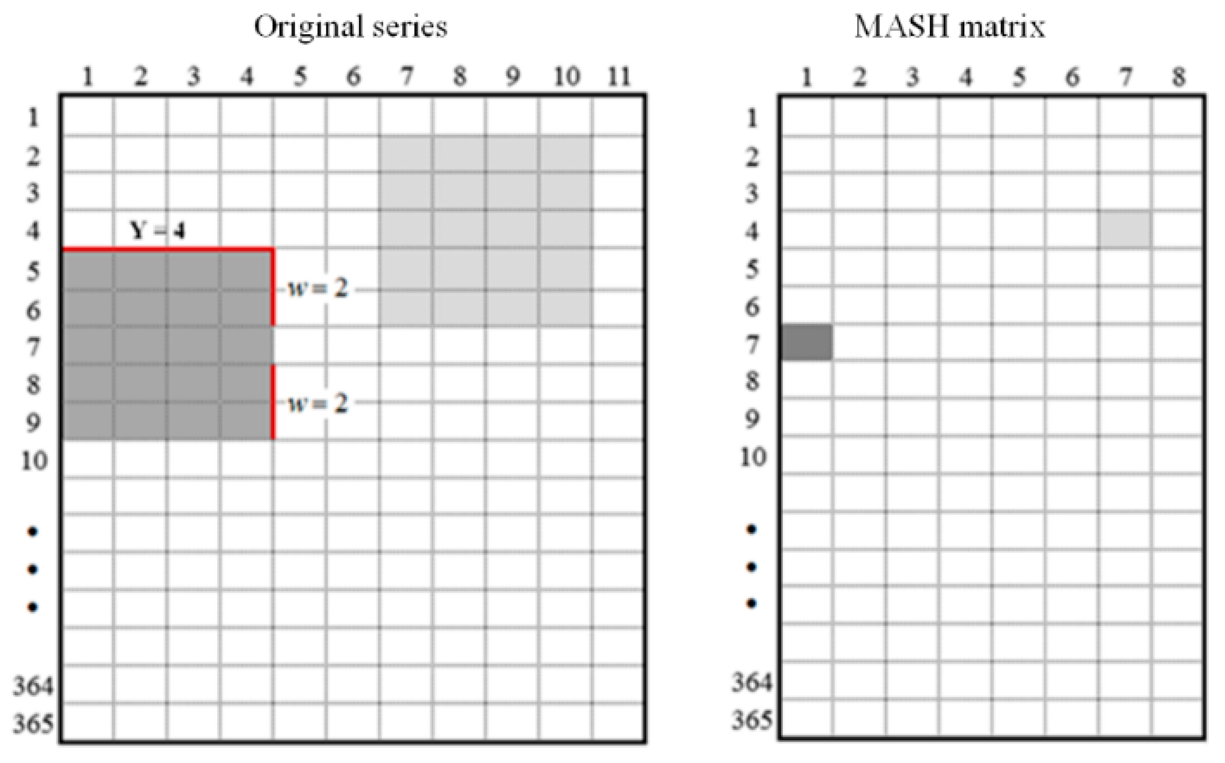
Moving average over shifting horizon (MASH), proposed by Anghileri et al. [13], is a non-parametric trend test method for seasonal data. The MASH method can show the intra- and inter-annual changes of data at the same time. The MASH method was first proposed to evaluate the intra- and inter-annual variation trend of daily streamflow time series. It can smooth the original streamflow time series by calculating the average value of continuous days over the same year and calculating the average streamflow of continuous years over the same day. Then the intra- and inter-annual variation trend of the original streamflow process can be illustrated. The purpose of MASH is to construct a matrix, as follows:
where represents the length of the resulting time series using MASH.
The moving average of the hth level on the tth day in the MASH matrix is calculated by
where represents the observed daily streamflow of the dth day in the yth year and Y and w represent the parameters of MASH, which indicate the size of the averaging window. For example, the process of MASH for an 11 year daily streamflow time series is shown in Figure 1.
The MASH method is equivalent to a low-pass filter. Through MASH, the original time series is transformed into a smoothed matrix that can characterize its seasonal trend. The smoothed results using MASH are affected by the two smoothing parameters Y and w. Small w values do not have a good smoothing effect on the daily streamflow data, while large w values may weaken the intra-annual variation of the time series excessively. The length of the resultant time series using MASH (Nh) is determined by Y and the number of years of the original time series:
2.3. Spearman Correlation Coefficient
The Spearman correlation coefficient is a statistical evaluation index that can evaluate the degree of correlation between two variables using the rank correlation theory [30,38]. The mathematical expression of the Spearman correlation coefficient is
where represents the rank difference between variable X and variable Y; and represent the rank of X and Y, respectively. indicates a positive correlation between X and Y while indicates a negative correlation. The larger the absolute value of the Spearman correlation coefficient, the stronger the correlation between the two variables.
2.4. Mann–Kendall Test
The MK test proposed by Mann [39] and Kendall [40] is a rank correlation analysis method. It is widely used in hydrometeorological trend analysis to test whether the trend of variables is significant [16,20,41]. Compared with the LR test, the MK test does not require the error to obey the normal distribution, and is affected by few outliers. For hydrological time series with n samples, the test statistic S is constructed as follows:
where x denotes a step function and S obeys the normal distribution. Its mean value is . The variance of S is calculated as follows:
The standard normal statistic Z, which is employed to assess the statistical significance, is constructed as follows:
A positive Z value indicates a rising trend while a negative Z value indicates a decreasing trend. By comparing Z with the standard normal cumulative distribution at a given significant level, the significance of a trend can be clarified. For the pre-set statistical test level , indicates a significant trend of the original time series while indicates a non-significant trend of the original time series. In addition, the p-value of the MK test can evaluate the significance of the trend quantitatively. The smaller the p-value is the smaller the probability of the original hypothesis occurring, indicating a more significant trend. Alternately, the greater the p-value is the greater the probability of original hypothesis occurring and the less significant the trend. This paper sets the significance level at . This means that when the results have passed the 95% significance test, and vice versa.
2.5. Sen’s Slope Estimation Method
The magnitude of the trend of the hydrological time series can be evaluated using Sen’s slope estimation method [42]. For hydrological time series with n samples , Sen’s slope estimation method assumes that the trend of the time series is linear and that the magnitude of the trend can be estimated as follows:
where is the median function. Sen’s slope estimation method is usually combined with the MK test. The MK test is employed to detect the significance of the trend of the time series while Sen’s slope estimation method is used to evaluate the magnitude of the trend.
3. Study Area and Data Collection
3.1. Study Area
The Jinsha River Basin originates from the upper reaches of the Yangtze River in China. The Jinsha River Basin flows through the five topographical geomorphic units of China including the Qinghai–Tibet Plateau, the Western Sichuan Plateau, the Hengduan Mountains, the Yunnan–Guizhou Plateau and the Southwestern Sichuan Basin [43]. The total length of the river is 3486 km, accounting for 77% of the total length of the upper reaches of the Yangtze River, and the control area of the river basin is 480,000 km2, accounting for 50% of the total area of the upper reaches of the Yangtze River [44,45]. The climate of the Jinsha River Basin has typical seasonal and regional differences and is influenced by plateau climates and stereoscopic climates [46].
During the winter half of the year (the northern section of Hengduan Mountains is from October to May of the next year, and the rest is from November to April of the next year) the Jinsha River Basin is mainly affected by westerly airflow, which is divided into two branches (southern and northern) by the Qinghai–Tibet Plateau. The southern branch passes through the Yunnan–Guizhou Plateau, bringing clear and dry continental weather. The northeastern part of the Jinsha River Basin is affected by the Kunming quasi-stationary front and southwestern airflow, bringing wet and rainy weather. During the summer half year (June–September or May–October) the westerly airflow retreats northward and the Jinsha River Basin is affected by southwest and southeast maritime monsoons, which bring abundant precipitation, and the rainfall belt decreases from the southeast to the northwest [47].
The distribution of the streamflow in the Jinsha River system corresponds to the distribution of the precipitation. The distribution characteristics are as follows: streamflow in the middle and lower reaches of the Jinsha River Basin has rapid growth, greater precipitation occurs in the mountain than the valley, and zonal horizontal distribution and vertical distribution of local areas are intertwined. For the lower reaches of the Jinsha River Basin (New Town–Yibin), mountainous areas lie on both sides of the reach. The annual precipitation is about 900–1300 mm, and the corresponding runoff depth is 500–900 mm. The upper and middle section belongs to the alpine gorge area. The annual precipitation is 600–800 mm, and the runoff depth is 400–700 mm. The annual precipitation in the valley area is only 400–600 mm and the runoff depth is only 200–400 mm. Due to global and regional warming in recent years, frequent floods and droughts have occurred in the Yangtze River Basin, which is where the Jinsha River Basin is located. The possibility of floods in the summer season and droughts in the fall is increasing. The possibility of summer floods and autumn droughts is growing [48].
The main stream of the Jinsha River is characterized by abundant runoff and stability, large river drop, abundant hydropower resources and acceptable development conditions. It is the largest hydropower energy base in China. The potential hydropower resources have reached 124 million kilowatts, accounting for about 16.7% of the total amount of China. The hydropower resources, which can be exploited, have reached 90 million kilowatts. With the construction and operation of "one reservoir and eight stages" cascade reservoirs (Longpan, Liangjiaren, Liyuan, Ahai, Jinanqiao, Longkaikou, Ludila and Guanyinyan) and four downstream cascade hubs (Wudongde, Baihetan, Xiluodu and Xiangjiaba), the temporal and spatial distribution of precipitation and runoff in the Jinsha River Basin has changed a lot. Therefore, it’s of great importance to research the intra- and inter-annual variability and changing trends of the hydrometeorological variables in the Jinsha River Basin.
3.2. Data Collection
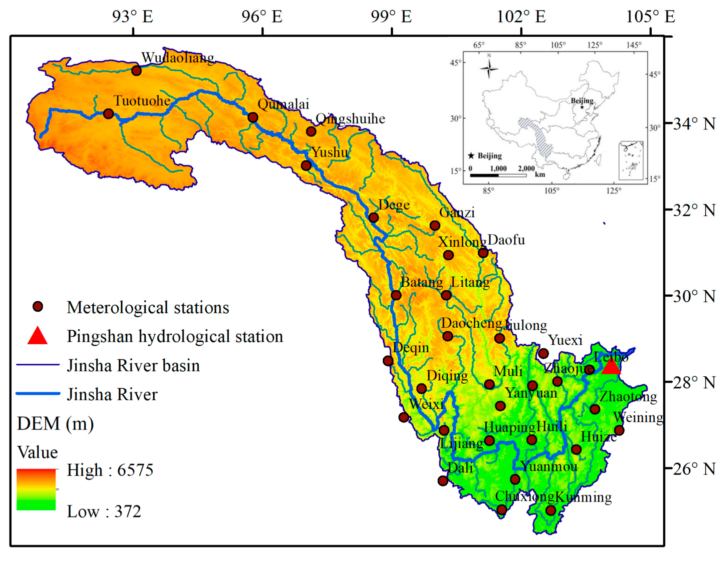
We selected the Jinsha River Basin as the study area. The mean daily streamflow, temperature and precipitation data of the Jinsha River Basin from 1974 to 2010 (37 years) were collected. The mean daily temperature and precipitation of the Jinsha River Basin were calculated based on 32 meteorological stations’ datasets in the Jinsha River Basin [49]. These meteorological stations’ datasets were collected from the National Meteorological Information Center (http://data.cma.cn/). To obtain the mean daily temperature and precipitation for the Jinsha River Basin at basin scale, the control area of each meteorological station was calculated using the Tyson polygon method. The mean daily temperature and precipitation for the whole Jinsha River Basin was obtained by calculating the weighted mean value of all stations. The mean daily temperature and precipitation were taken as the daily temperature and precipitation for the Jinsha River Basin for the next subsequent analysis. The streamflow of the control station (Pingshan) of the Jinsha River Basin was taken as the mean daily streamflow of the Jinsha River Basin. The streamflow data of the Pingshan hydrological station was obtained from the Bureau of Hydrology, Changjiang Water Resources Commission, Wuhan, China. The location of the Jinsha River Basin, the Pingshan hydrological station and the 32 meteorological stations in the basin are shown in Figure 2.
According to the statistical analysis of the historical hydrometeorological data (Figure 3), the mean annual temperature of the Jinsha River Basin from 1974 to 2010 was 6.1 °C. The coldest month was January (−3.4 °C) and the warmest was July (14.2 °C). The mean annual sum of precipitation was 628.40 mm. The highest mean monthly sum of precipitation was measured in July (141.59 mm) and the lowest was in December (3.62 mm). The precipitation was mainly concentrated between June and September. The mean annual sum of streamflow was 167,000 m3/s. The highest mean monthly sum of streamflow was measured in August (30,059 m3/s) and the lowest was in February (4229 m3/s).
4. Results and Discussion
4.1. MK Trend Detection Results
The MK trend detection results for mean temperature, precipitation and streamflow in the Jinsha River Basin from 1974 to 2010 are shown in Table 1. The mean annual streamflow (temperature and precipitation) was calculated by averaging the daily streamflow per year and the mean monthly streamflow was calculated by averaging the daily streamflow per month. The level of significance chosen was . When , the test result of the MK method was significant. The MK trend detection results included the statistics of S and Z, the estimated Sen’s slope b and the significance index p-value.
From the MK trend detection results for temperature in Table 1, we found that the annual temperature showed a significant increasing trend. The monthly temperature showed significant increasing trends for January, March through September, November and December, but non-significant increasing trends for February and October. The detected results for temperature were consistent with the global warming background. From the MK trend detection results for precipitation in Table 1, we found that the annual precipitation showed a non-significant increasing trend. The monthly precipitation showed decreasing trends for April, September and December, and increasing trends for the other months. All the increasing or decreasing trends were not significant for precipitation time series. Under the regional warming background, the atmospheric circulation situation of the Jinsha River Basin has changed, which may be the reason for the decreasing or increasing precipitation trends. From the MK trend detection results for streamflow in Table 1, we found that the annual streamflow from 1974 to 2010 for the Jinsha River Basin showed a non-significant increasing trend. The monthly streamflow showed non-significant decreasing trends for June and October. For the other months the trends were increasing. The increasing trends were significant between January and April and non-significant between May and July, and in November and December. Since the streamflow of the Jinsha River Basin originates from snow melting and, mainly, from rainfall, the increased temperature, consequently, caused increased streamflow for most of the months. Because there is a time delay between precipitation and streamflow in the water cycle, the decreasing streamflow of June and October can be explained by the decreasing precipitation in the previous one or two months. What is more, the formation of streamflow in nature is complex and affected by other factors such as snow melting and water conservancy projects.
4.2. Results of the MASH Method
To further investigate the intra- and inter-annual variability of the hydrometeorological variables in the Jinsha River Basin, the MASH method was introduced to smooth the hydrometeorological variables and display their intra- and inter-annual variability visually. The daily temperature, precipitation and streamflow time series, from 1974 to 2010, of the Jinsha River Basin were smoothed using the MASH method. By setting , and the number of years of the original time series (), the number of the patterns of the MASH matrix were computed as , as per Equation (3). By taking temperature as an example, of the 28 MASH patterns the first MASH pattern was the smoothed temperature computed over the horizon from 1974 to 1983, the second MASH pattern was the smoothed temperature computed over the horizon from 1975 to 1984, etc. The smoothed temperature, precipitation and streamflow are shown in Figure 4. Older horizons were plotted with blue lines and more recent horizons with red lines.
Shown in Figure 4, the inter-annual variation characteristics of the hydrometeorological variables can be clarified by comparing their trends over different years in the same day, and the intra-annual variation characteristics can be clarified by comparing their trends over different days in one year. As is illustrated in Figure 4a, the temperature generally showed an increasing trend from 1974 to 2010 on the same day, and the increase in temperature was very small. As shown in Figure 4b, the precipitation generally showed an increasing trend from 1974 to 2010 on the same day. The increase in precipitation in May, July and August was large, and a decreasing trend occurred in September. As in Figure 4c, we noted that the streamflow of 1990s (light red or yellow) was the largest, that of the 2000s (dark red) or 1980s (light blue) was the second largest, and that of the 1970s (dark blue) was the smallest. In the summer of 1998, the entire Yangtze River Basin suffered tremendous flooding. The 1998 Great Flood caused serious losses in industry and agriculture to the Yangtze River Basin [50]. According to Fluixá-Sanmartín et al. [51], an extreme drought event was observed from 1978 to 1979. A total number of 7000 km2 of agricultural land was seriously affected. Figure 4c also shows that the increase in streamflow from July to early September of the 1990s was relatively large compared with the 1970s and 1980s. From mid-September to early October, the streamflow showed a decreasing trend.
As for the intra-annual variation characteristics, we found that the highest precipitation occurred from June to September, which resulted in high streamflow in summer and autumn. Lower precipitation was observed in spring and winter, which resulted in less streamflow. The temperature gradually increased from January to mid-July, and the highest temperature, observed in mid-July, was 15 °C. The temperature then gradually decreased from mid-July to December.
Figure 5 is another way to show the results of MASH, which can illustrate the duration of different hydrometeorological processes intuitively, instead of the variations in variable magnitude. The magnitude of different hydrometeorological variables is illustrated using a color scale. Figure 5a clearly demonstrates that higher temperatures (>10 °C) were measured from June to September from 1974 to 2010. From Figure 5b, we see that higher precipitation (>4.5 mm) was measured in July from the 20th to the 25th horizon, which corresponds to the years 1993 to 2007. As is shown in Figure 5c, higher streamflow (>1000 m3/s) was measured in September, from the 17th to the 28th horizon, which corresponded to the years 1990 through 2010.
To analyze the correlation between hydrometeorological variables and test the influence of the MASH method on the correlation between two variables, the Spearman correlation coefficients for the smoothed hydrometeorological variables and the original hydrometeorological variables were given in Table 2. It can be seen from Table 2 that the range of the negative Spearman correlation coefficients for smoothed streamflow and precipitation was (−0.82, −0.15) while that of the positive was (0.16, 0.98). The Spearman correlation coefficient between the smoothed annual streamflow and precipitation was relatively large, reaching 0.98. The range of the negative Spearman correlation coefficients for smoothed streamflow and temperature was (−0.52, 0.08) while that of the positive was (0.34, 0.95). The Spearman correlation coefficient between the smoothed annual streamflow and temperature was relatively large, reaching 0.85. Further review of Table 2 showed that the correlation between the smoothed data was significantly greater than that between the original hydrometeorological data for annual data and most monthly data, except for the October temperature, and April and September precipitation, indicating that the MASH method smoothed data and eliminated the periodic variation and random fluctuation of the original time series. It then extracted useful information that showed the regularity and trend of the original time series.
4.3. Combination of the MASH Method with Statistical Tests
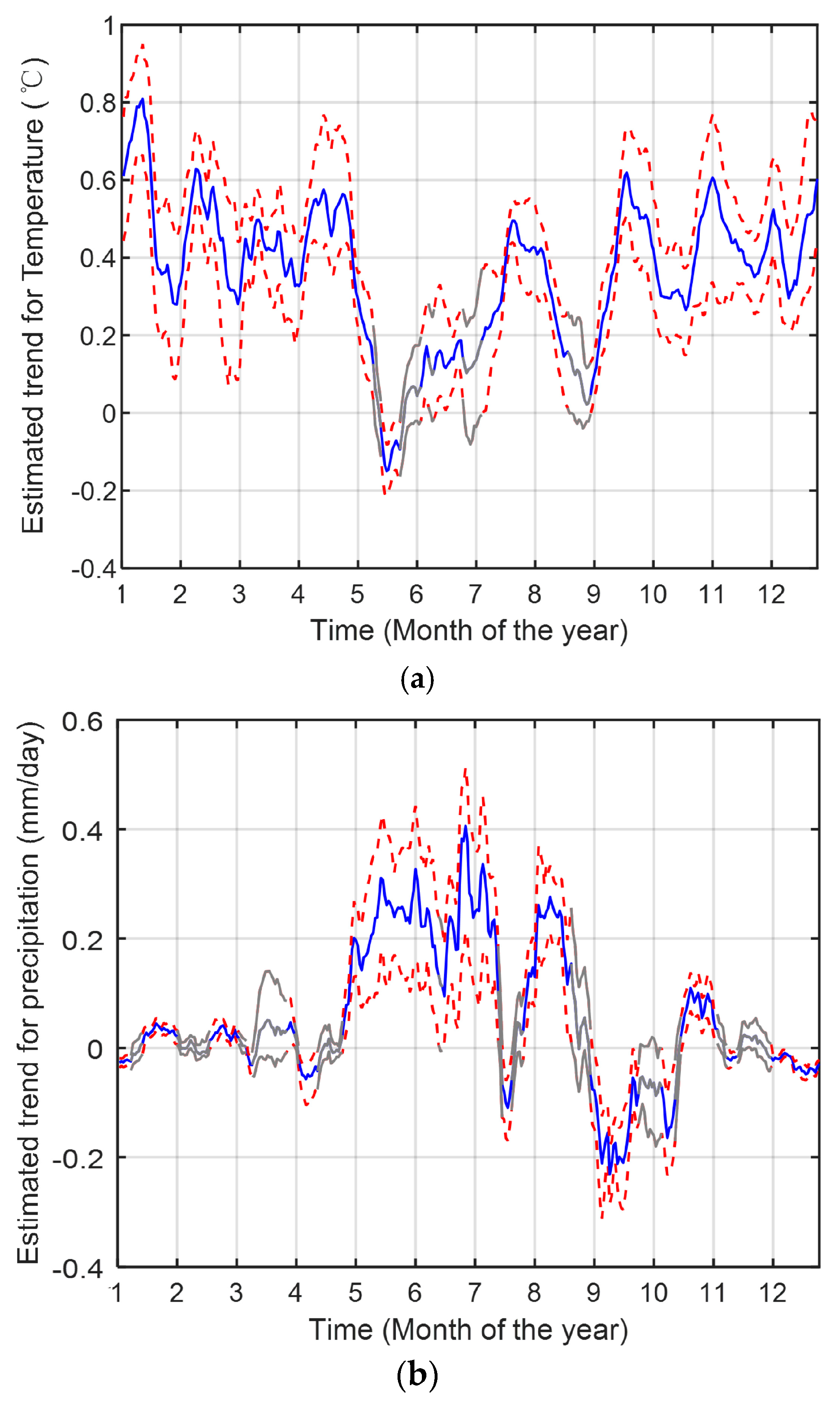
The smoothed MASH matrix was analyzed using the MK test for trend detection. Figure 6 shows the MK trend detection results for the MASH matrix of 31 days over a 10 year horizon for temperature, precipitation and streamflow, respectively. Solid blue lines represent the trend estimated using Sen’s slope estimation of temperature, precipitation and streamflow for the 28 total MASH horizons at 0.05 significance. The dotted line represents the 95% confidence bounds of Sen’s slope estimation. The grey lines indicate that the estimated slopes are insignificant. Alternately, the red or blue lines indicate that the estimated slopes are significant.
As can be seen for temperature, Figure 6a, the estimated Sen’s slope for a few days in mid-May was smaller than 0, which indicated decreasing trends. The estimated slope for the remaining days of the year was bigger than 0, which indicated increasing trends. The highest changes in temperature were estimated in early January, with a peak of 0.8 ℃. As can be seen for precipitation, Figure 6b, decreasing trends were detected from early September to early October while the rest of the year showed increasing trends. The highest changes in temperature were estimated in late June, with a peak of 0.4 mm/day. As can be seen for streamflow, Figure 6c, decreasing trends were detected from mid-September to late October. Increasing trends were detected the rest of the year. The highest changes in streamflow were estimated in mid-August, with a peak of 138 m3/s. Compared with the trend detection results for streamflow and temperature, the non-significant days for precipitation were more numerous (more grey dots).
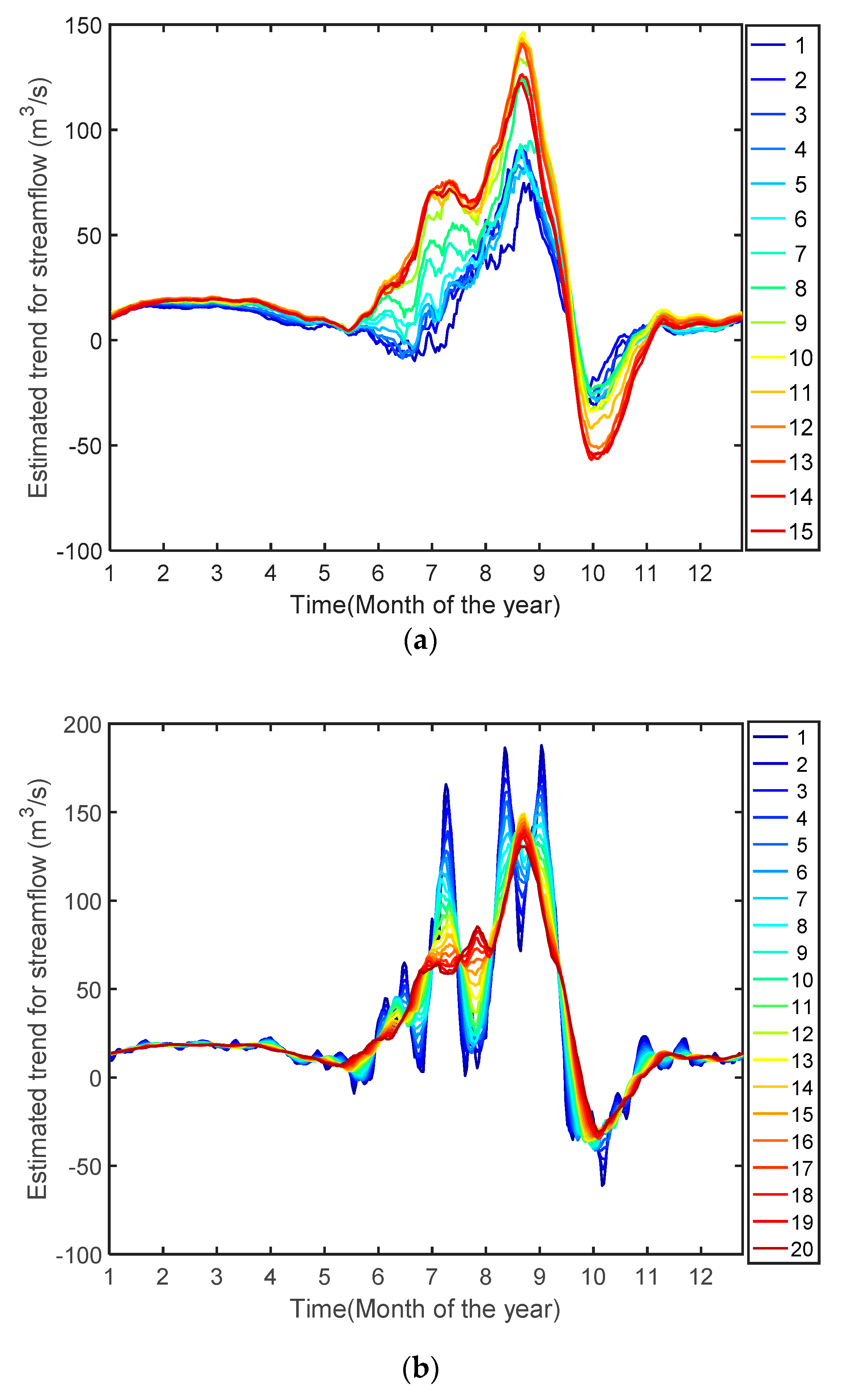
4.4. Sensitivity Analysis of the Smoothing Parameters on Estimated Trends
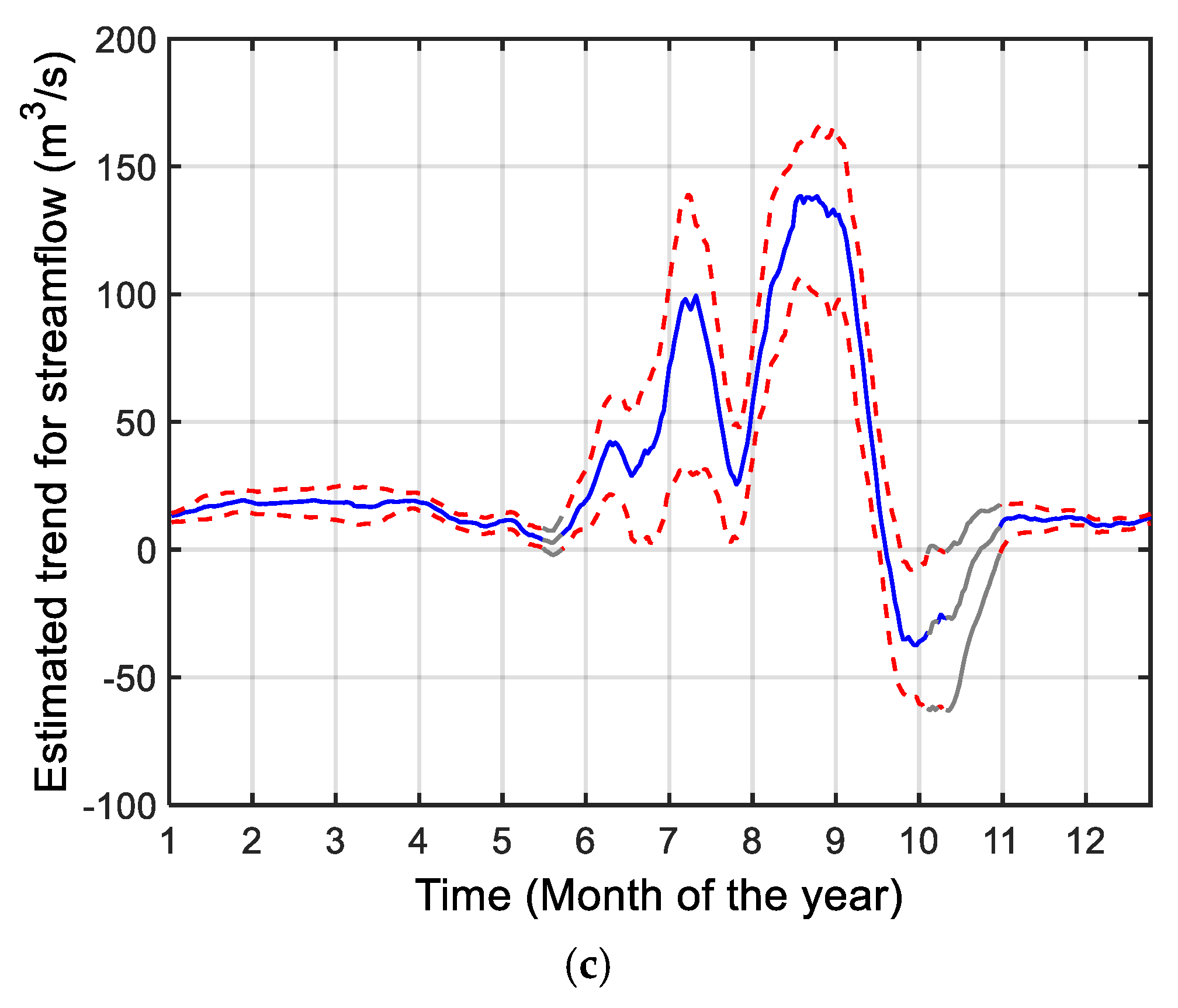
Since the estimated trend was sensitive to the choice of smoothing parameters, sensitivity analysis of the selection of smoothing parameters of w and Y was performed to increase the robustness of the estimated trends. The sensitivity analysis was performed by analyzing the influence of the smoothing parameters on the estimated trends. The estimated trends, based on Sen’s slope, were calculated under different w and Y parameters. We utilized the MASH results of streamflow time series as an example. The influences of the Y and w parameters on estimated trends are illustrated in Figure 7a,b respectively. To analyze the influences of the Y parameter, the w parameter remained at 15 while the Y parameter varied from 1 to 15 (Figure 7a). The estimated trends were nearly the same throughout the year, except for the period between early June and early July when negative trends were estimated when Y was set as 1 or 2.
To analyze the influence of the w parameter, the Y parameter remained at 10 while the w parameter varied from 1 (average window of 3 days) to 20 (average window of 41 days) (Figure 7b). The estimated trends were almost the same throughout the year, except for May when negative trends were estimated when Y was set as 1. Figure 7b shows that the day-to-day variability of the smoothed time series, the blue lines (w was set from 1 to 6), fluctuated significantly. Lager w values, alternately, resulted in smoother trend results.
5. Conclusions
In this study, the MASH method was combined with the MK test and Sen’s slope estimation to investigate the inter- and intra-annual variability in daily streamflow, precipitation and temperature time series from 1974 to 2010 for the Jinsha River Basin. The Spearman correlation coefficients for the original and smoothed hydrometeorological time series were compared to demonstrate the influence of the MASH method, filtering out the fluctuations and periodicity of variables. Sensitivity analysis of the smoothing parameters on estimated trends was performed. The main conclusions of this study are summarized as follows:
- The annual temperature from 1974 to 2010 showed a significant increasing trend. Significant increasing trends were detected for almost all of the monthly temperatures, except February and October. Significant increasing trends were detected from January to April for streamflow. The increasing temperature was consistent with the global warming background. Temperature variations played an important role in the formation of streamflow and explained the increasing trends for streamflow.
- The intra- and inter-annual variability of hydrometeorological time series and the duration of different hydrometeorological variables were obtained via analyses of the MASH results. The temperature, precipitation and streamflow from 1974 to 2010 showed increasing inter-annual variability most of the days over each year period. Compared with the 1970s and 1980s, the increase in streamflow from early July to early September of the 1990s was considerable. For precipitation, the increase in May, July and August of the 1990s was notable. The correlation coefficients between smoother hydrometeorological variables were generally larger than those between the original hydrometeorological variables, which indicated that the MASH method smoothed the data and eliminated the effects of periodic changes and random fluctuations in hydrometeorological time series. The regularity and trends of the hydrometeorological data could then be detected.
- The combination of the MASH with the MK test showed the largest estimated changes in temperature in early January, with a peak of 0.8 ℃. The highest estimated changes in precipitation were in late June, with a peak of 0.4 mm/day. The highest estimated changes in streamflow were in mid-August, with a peak of 138 m3/s.
- Sensitivity analysis of the smoothing parameters on was performed to increase the robustness of the estimated trends. For different Y values, the estimated trends were nearly the same throughout the year except when Y was set as 1 or 2. For different w values, the estimated trends were nearly the same throughout the year, except when w was set as 1. Due to the day-to-day variability of the smoothed time series, small w (1 to 6) values resulted in fluctuating trend results.
This study combined the MASH method with the MK test and Sen’s slope method to investigate the inter- and intra-annual variability of hydrometeorological variables in the Jinsha River Basin. The MASH results were obtained by calculating the ‘mean’ value of continuous days over the same year and of continuous years over the same day. The ‘median’ value was considered to replace the ‘mean’ value in future research. The combination of MASH with other statistical tests, such as the seasonal MK test, can also be researched. What is more, the MASH method can be applied to other catchments for trend analyses in future studies.
Author Contributions
C.Z. designed the experiments and gave constructive advice; T.P. collected the data, performed the experiments and wrote a first draft; J.Z. proposed the basic concepts and made corrections; Xiaolu Wang collected relevant material and gave advice for advisement.
Funding
This research received no external funding.
Acknowledgments
This work was supported by the Natural Science Foundation of the Jiangsu Higher Education Institution of China (No. 19KJB480007), the Natural Science Foundation of the Jiangsu Higher Education Institution of China (No. 19KJB470012), the National Natural Science Foundation of China (NSFC) (No. 51709121), the National Natural Science Foundation of China (No. 51709122) and the National Natural Science Foundation of China (No. 51741907).
Conflicts of Interest
The authors declare no conflicts of interest.
References
- Adarsh, S.; Janga Reddy, M. Trend analysis of rainfall in four meteorological subdivisions of southern India using nonparametric methods and discrete wavelet transforms. Int. J. Climatol. 2015, 35, 1107–1124. [Google Scholar] [CrossRef]
- Senent-Aparicio, J.; Liu, S.; Pérez-Sánchez, J.; López-Ballesteros, A.; Jimeno-Sáez, P. Assessing Impacts of Climate Variability and Reforestation Activities on Water Resources in the Headwaters of the Segura River Basin (SE Spain). Sustainability 2018, 10, 3277. [Google Scholar] [CrossRef]
- Tian, P.; Zhou, J.; Chu, Z.; Na, S. Modeling and Combined Application of Orthogonal Chaotic NSGA-II and Improved TOPSIS to Optimize a Conceptual Hydrological Model. Water Resour. Manag. 2018, 32, 3781–3799. [Google Scholar]
- Li, F.; Zhang, G.; Xu, Y.J. Spatiotemporal variability of climate and streamflow in the Songhua River Basin, northeast China. J. Hydrol. 2014, 514, 53–64. [Google Scholar] [CrossRef]
- Zhang, Y.; You, Q.; Lin, H.; Chen, C. Analysis of dry/wet conditions in the Gan River Basin, China, and their association with large-scale atmospheric circulation. Glob. Planet. Chang. 2015, 133, 309–317. [Google Scholar] [CrossRef]
- Zhang, C.; Peng, T.; Li, C.; Fu, W.; Xia, X.; Xue, X. Multiobjective Optimization of a Fractional-Order PID Controller for Pumped Turbine Governing System Using an Improved NSGA-III Algorithm under Multiworking Conditions. Complexity 2019, 2019, 1–18. [Google Scholar] [CrossRef]
- Zhang, C.; Li, C.; Peng, T.; Xia, X.; Xue, X.; Fu, W.; Zhou, J. Modeling and Synchronous Optimization of Pump Turbine Governing System Using Sparse Robust Least Squares Support Vector Machine and Hybrid Backtracking Search Algorithm. Energies 2018, 11, 3108. [Google Scholar] [CrossRef]
- Stocker, T.F.; Qin, D.; Plattner, G.-K.; Tignor, M.M.; Allen, S.K.; Boschung, J.; Nauels, A.; Xia, Y.; Bex, V.; Midgley, P.M. IPCC, 2013: Climate Change 2013: The physical science basis. contribution of working group I to the fifth assessment report of IPCC the intergovernmental panel on climate change; Cambridge University Press: Cambridge, UK, 2014. [Google Scholar]
- Xu, L.; Shi, Z.; Wang, Y.; Zhang, S.; Chu, X.; Yu, P.; Xiong, W.; Zuo, H.; Wang, Y. Spatiotemporal variation and driving forces of reference evapotranspiration in Jing River Basin, northwest China. Hydrol. Process. 2015, 29, 4846–4862. [Google Scholar] [CrossRef]
- Feng, X.; Cheng, W.; Fu, B.; Lü, Y. The role of climatic and anthropogenic stresses on long-term runoff reduction from the Loess Plateau, China. Sci. Total Environ. 2016, 571, 688–698. [Google Scholar] [CrossRef]
- Nilsson, C.; Reidy, C.A.; Dynesius, M.; Revenga, C. Fragmentation and flow regulation of the world’s large river systems. Science 2005, 308, 405. [Google Scholar] [CrossRef]
- Tukey, J.W. EDA: Exploratory data analysis; Addison-Wesley: Reading, MA, USA, 1977. [Google Scholar]
- Anghileri, D.; Pianosi, F.; Soncini-Sessa, R. Trend detection in seasonal data: from hydrology to water resources. J. Hydrol. 2014, 511, 171–179. [Google Scholar] [CrossRef]
- Pandey, B.K.; Khare, D. Identification of trend in long term precipitation and reference evapotranspiration over Narmada river basin (India). Glob. Planet. Chang. 2018, 161, 172–182. [Google Scholar] [CrossRef]
- Pavlić, K.; Parlov, J. Cross-Correlation and Cross-Spectral Analysis of the Hydrographs in the Northern Part of the Dinaric Karst of Croatia. Geosciences 2019, 9, 86. [Google Scholar] [CrossRef]
- Mengistu, D.; Bewket, W.; Lal, R. Recent spatiotemporal temperature and rainfall variability and trends over the Upper Blue Nile River Basin, Ethiopia. Int. J. Climatol. 2014, 34, 2278–2292. [Google Scholar] [CrossRef]
- Feidas, H. Trend analysis of air temperature time series in Greece and their relationship with circulation using surface and satellite data: Recent trends and an update to 2013. Theor. Appl. Climatol. 2017, 129, 1383–1406. [Google Scholar] [CrossRef]
- Pavlić, K.; Kovač, Z.; Jurlina, T. Trend analysis of mean and high flows in response to climate warming-Evidence from karstic catchments in Croatia. Geofizika 2017, 34, 157–174. [Google Scholar] [CrossRef]
- Mahmood, R.; Jia, S. Assessment of hydro-climatic trends and causes of dramatically declining stream flow to Lake Chad, Africa, using a hydrological approach. Sci. Total Environ. 2019, 675, 122–140. [Google Scholar] [CrossRef]
- Gocic, M.; Trajkovic, S. Analysis of changes in meteorological variables using Mann-Kendall and Sen’s slope estimator statistical tests in Serbia. Glob. Planet. Chang. 2013, 100, 172–182. [Google Scholar] [CrossRef]
- Li, F.; Zhang, G.; Xu, Y.J. Separating the Impacts of Climate Variation and Human Activities on Runoff in the Songhua River Basin, Northeast China. Water 2014, 6, 3320–3338. [Google Scholar] [CrossRef] [Green Version]
- Pandey, B.K.; Tiwari, H.; Khare, D. Trend analysis using discrete wavelet transform (DWT) for long-term precipitation (1851–2006) over India. Hydrol. Sci. J. 2017, 62, 2187–2208. [Google Scholar] [CrossRef]
- Sang, Y.-F.; Wang, Z.; Liu, C. Comparison of the MK test and EMD method for trend identification in hydrological time series. J. Hydrol. 2014, 510, 293–298. [Google Scholar] [CrossRef]
- Jukić, D.; Denić-Jukić, V. Partial spectral analysis of hydrological time series. J. Hydrol. 2011, 400, 223–233. [Google Scholar] [CrossRef]
- Jukić, D.; Denić-Jukić, V. Investigating relationships between rainfall and karst-spring discharge by higher-order partial correlation functions. J. Hydrol. 2015, 530, 24–36. [Google Scholar] [CrossRef]
- Fu, W.; Wang, K.; Zhou, J.; Xu, Y.; Tan, J.; Chen, T. A Hybrid Approach for Multi-Step Wind Speed Forecasting Based on Multi-Scale Dominant Ingredient Chaotic Analysis, KELM and Synchronous Optimization Strategy. Sustainability 2019, 11, 1804. [Google Scholar] [CrossRef]
- Fu, W.; Wang, K.; Li, C.; Tan, J. Multi-step short-term wind speed forecasting approach based on multi-scale dominant ingredient chaotic analysis, improved hybrid GWO-SCA optimization and ELM. Energy Convers. Manag. 2019, 187, 356–377. [Google Scholar] [CrossRef]
- Araghi, A.; Baygi, M.M.; Adamowski, J.; Malard, J.; Nalley, D.; Hasheminia, S.M. Using wavelet transforms to estimate surface temperature trends and dominant periodicities in Iran based on gridded reanalysis data. Atmos. Res. 2015, 155, 52–72. [Google Scholar] [CrossRef]
- Huang, N.E.; Shen, Z.; Long, S.R.; Wu, M.C.; Shih, H.H.; Zheng, Q.; Yen, N.-C.; Tung, C.C.; Liu, H.H. The empirical mode decomposition and the Hilbert spectrum for nonlinear and non-stationary time series analysis. Proc. R. Soc. Lond. Ser. A Math. Phys. Eng. Sci. 1998, 454, 903–995. [Google Scholar] [CrossRef]
- Zhang, C.; Zhou, J.; Li, C.; Fu, W.; Peng, T. A compound structure of ELM based on feature selection and parameter optimization using hybrid backtracking search algorithm for wind speed forecasting. Energy Convers. Manag. 2017, 143, 360–376. [Google Scholar] [CrossRef]
- Zhang, Q.; Singh, V.P.; Li, K.; Li, J. Trend, periodicity and abrupt change in streamflow of the East River, the Pearl River basin. Hydrol. Process. 2014, 28, 305–314. [Google Scholar] [CrossRef]
- Peng, T.; Zhou, J.; Zhang, C.; Zheng, Y. Multi-step ahead wind speed forecasting using a hybrid model based on two-stage decomposition technique and AdaBoost-extreme learning machine. Energy Convers. Manag. 2017, 153, 589–602. [Google Scholar] [CrossRef]
- Wang, W.C.; Chau, K.W.; Qiu, L.; Chen, Y.B. Improving forecasting accuracy of medium and long-term runoff using artificial neural network based on EEMD decomposition. Environ. Res. 2015, 139, 46. [Google Scholar] [CrossRef] [PubMed]
- Smith, R.L. Extreme value analysis of environmental time series: an application to trend detection in ground-level ozone. Stat. Sci. 1989, 4, 367–377. [Google Scholar] [CrossRef]
- Kousari, M.R.; Ahani, H.; Hendi-zadeh, R. Temporal and spatial trend detection of maximum air temperature in Iran during 1960–2005. Glob. Planet. Chang. 2013, 111, 97–110. [Google Scholar] [CrossRef]
- Osuch, M.; Wawrzyniak, T. Inter- and intra-annual changes in air temperature and precipitation in western Spitsbergen. Int. J. Climatol. 2016, 37, 3082–3097. [Google Scholar] [CrossRef]
- Osuch, M.; Wawrzyniak, T. Variations and changes in snow depth at meteorological stations Barentsburg and Hornsund (Spitsbergen). Ann. Glaciol. 2017, 58, 11–20. [Google Scholar] [CrossRef] [Green Version]
- Horn, P. Introduction to Robust Estimation and Hypothesis Testing. Technometrics 2012, 40, 77–78. [Google Scholar] [CrossRef]
- Mann, H.B. Nonparametric Tests Against Trend. Econometrica 1945, 13, 245–259. [Google Scholar] [CrossRef]
- Kendall, M. Rank Correlation Methods; Charles Griffin & Company Ltd.: London/High Wycombe, UK, 1975. [Google Scholar]
- Tan, M.L.; Chua, V.P.; Li, C.; Brindha, K. Spatiotemporal analysis of hydro-meteorological drought in the Johor River Basin, Malaysia. Theor. Appl. Climatol. 2019, 135, 825–837. [Google Scholar] [CrossRef]
- Sen, P.K. Estimates of the regression coefficient based on Kendall’s tau. J. Am. Stat. Assoc. 1968, 63, 1379–1389. [Google Scholar] [CrossRef]
- Tayyab, M.; Zhou, J.; Zeng, X.; Adnan, R. Discharge forecasting by applying artificial neural networks at the Jinsha river basin, China. Eur. Sci. J. ESJ 2016, 12, 108–127. [Google Scholar] [CrossRef]
- Peng, T.; Zhou, J.; Zhang, C.; Fu, W. Streamflow Forecasting Using Empirical Wavelet Transform and Artificial Neural Networks. Water 2017, 9, 406. [Google Scholar] [CrossRef]
- Zhou, J.; Peng, T.; Zhang, C.; Sun, N. Data Pre-Analysis and Ensemble of Various Artificial Neural Networks for Monthly Streamflow Forecasting. Water 2018, 10, 628. [Google Scholar] [CrossRef]
- Hairong, Z.; Jianzhong, Z.; Xiaofan, Z.; Yi, L.; Jun, G. Application of One-way coupled Hydro-meteorological Model in the Jinshajiang River Basin, China. In Proceedings of the 2nd International Conference on Architectural, Civil and Hydraulics Engineering (ICACHE 2016), Kunming, China, 29–30 September 2016. [Google Scholar]
- Zhou, J.; Zhang, H.; Zhang, J.; Zeng, X.; Ye, L.; Liu, Y.; Tayyab, M.; Chen, Y. WRF model for precipitation simulation and its application in real-time flood forecasting in the Jinshajiang River Basin, China. Meteorol. Atmos. Phys. 2018, 130, 635–647. [Google Scholar] [CrossRef]
- Zhang, Q.; Xu, C.-Y.; Zhang, Z.; Chen, Y.D.; Liu, C.-l.; Lin, H. Spatial and temporal variability of precipitation maxima during 1960–2005 in the Yangtze River basin and possible association with large-scale circulation. J. Hydrol. 2008, 353, 215–227. [Google Scholar] [CrossRef]
- Tayyab, M.; Zhou, J.; Dong, X.; Ahmad, I.; Sun, N. Rainfall-runoff modeling at Jinsha River basin by integrated neural network with discrete wavelet transform. Meteorol. Atmos. Phys. 2019, 131, 115–125. [Google Scholar] [CrossRef]
- Yin, H.; Changan, L.I. Human impact on floods and flood disasters on the Yangtze River. Geomorphology 2001, 41, 105–109. [Google Scholar] [CrossRef]
- Fluixá-Sanmartín, J.; Deng, P.; Fischer, L.; Orlowsky, B.; García-Hernández, J.; Jordan, F.; Haemmig, C.; Zhang, F.; Xu, J. Searching for the optimal drought index and timescale combination to detect drought: A case study from the lower Jinsha River basin, China. Hydrol. Earth Syst. Sci. Discuss. 2018, 22, 1–30. [Google Scholar] [CrossRef]
Figure 1.
A scheme of the moving average over shifting horizon (MASH) process (Y = 4, w = 2, Ny = 11) represents the number of years of the original time series, and Nh = 8 represents the length of the resultant time series of MASH).
Figure 1.
A scheme of the moving average over shifting horizon (MASH) process (Y = 4, w = 2, Ny = 11) represents the number of years of the original time series, and Nh = 8 represents the length of the resultant time series of MASH).

Figure 2.
The Jinsha River Basin in Southwest China and the hydrological (triangle) and meteorological (dots) stations used in this study.
Figure 2.
The Jinsha River Basin in Southwest China and the hydrological (triangle) and meteorological (dots) stations used in this study.

Figure 3.
Mean monthly temperature, precipitation and streamflow for the Jinsha River Basin from 1974 to 2010. (a) Mean monthly temperature; (b) Mean monthly precipitation and streamflow.
Figure 3.
Mean monthly temperature, precipitation and streamflow for the Jinsha River Basin from 1974 to 2010. (a) Mean monthly temperature; (b) Mean monthly precipitation and streamflow.

Figure 4.
The MASH results of daily temperature, precipitation and streamflow ( years and days, time horizon 1974–2010). (a) temperature; (b) precipitation; (c) streamflow.
Figure 4.
The MASH results of daily temperature, precipitation and streamflow ( years and days, time horizon 1974–2010). (a) temperature; (b) precipitation; (c) streamflow.

Figure 5.
The MASH time representation of temperature, precipitation and streamflow from 1974 to 2010. (a) temperature; (b) precipitation; (c) streamflow.
Figure 5.
The MASH time representation of temperature, precipitation and streamflow from 1974 to 2010. (a) temperature; (b) precipitation; (c) streamflow.

Figure 6.
The MK test of trend detection for the MASH matrix of temperature, precipitation and streamflow from 1974 to 2010. The solid blue lines represent the estimated trend based on Sen’s slope. The dotted line represents the 95% confidence bounds. The grey lines indicate insignificant trends and the red or blue lines indicate significant trends. (a) temperature; (b) precipitation; (c) streamflow.


Figure 7.
Influence of smoothing parameters on estimated trends for smoothed streamflow. (a) Influence of Y parameter on estimated trends; (b) Influence of w parameter on estimated trends.
Figure 7.
Influence of smoothing parameters on estimated trends for smoothed streamflow. (a) Influence of Y parameter on estimated trends; (b) Influence of w parameter on estimated trends.


Table 1.
Mann–Kendall (MK) test (test statistics S, Z and Sen’s slope b) results for annual and monthly temperature, precipitation and streamflow at 5% significance level.
Table 1.
Mann–Kendall (MK) test (test statistics S, Z and Sen’s slope b) results for annual and monthly temperature, precipitation and streamflow at 5% significance level.
| Time Scale | Temperature | Precipitation | Streamflow | ||||||
|---|---|---|---|---|---|---|---|---|---|
| S | Z | b | S | Z | b | S | Z | b | |
| Year | 338 | 4.408 | 0.035 * | 124 | 1.609 | 0.004 | 114 | 1.478 | 1.500 |
| January | 246 | 3.204 | 0.063 * | 78 | 1.007 | 0.001 | 298 | 3.884 | 1.640 * |
| February | 134 | 1.739 | 0.044 | 36 | 0.458 | 0.001 | 288 | 3.754 | 1.526 * |
| March | 218 | 2.838 | 0.040 * | 12 | 0.144 | 0.001 | 328 | 4.277 | 1.522 * |
| April | 248 | 3.230 | 0.033 * | −24 | −0.301 | −0.001 | 151 | 1.962 | 0.749 * |
| May | 174 | 2.263 | 0.024 * | 104 | 1.347 | 0.012 | 56 | 0.719 | 0.494 |
| June | 160 | 2.080 | 0.022 * | 22 | 0.275 | 0.004 | −8 | −0.092 | −0.124 |
| July | 282 | 3.675 | 0.039 * | 88 | 1.138 | 0.012 | 12 | 0.144 | 0.716 |
| August | 228 | 2.969 | 0.030 * | 80 | 1.033 | 0.012 | 74 | 0.955 | 4.232 |
| September | 236 | 3.074 | 0.043 * | −128 | −1.661 | −0.014 | 60 | 0.772 | 3.778 |
| October | 134 | 1.739 | 0.027 | 64 | 0.824 | 0.007 | −44 | −0.562 | −1.808 |
| November | 166 | 2.158 | 0.026 * | 2 | 0.013 | 0.000 | 48 | 0.615 | 0.625 |
| December | 218 | 2.838 | 0.041* | −64 | −0.824 | −0.001 | 62 | 0.798 | 0.448 |
* indicates a significant trend at 5% significance level for MK test.
Table 2.
Pearson correlation coefficients for smoothed time series (streamflow vs. precipitation, streamflow vs. temperature) and original time series (streamflow vs. precipitation, streamflow vs. temperature) in annual and monthly time scale.
Table 2.
Pearson correlation coefficients for smoothed time series (streamflow vs. precipitation, streamflow vs. temperature) and original time series (streamflow vs. precipitation, streamflow vs. temperature) in annual and monthly time scale.
| Time Scale | Year | Jan. | Feb. | Mar. | Apr. | May. | Jun. | Jul. | Aug. | Sep. | Oct. | Nov. | Dec. |
|---|---|---|---|---|---|---|---|---|---|---|---|---|---|
| Smoothed series | streamflow vs. precipitation | ||||||||||||
| 0.98 | 0.65 | 0.42 | 0.16 | −0.15 | 0.89 | 0.93 | 0.92 | 0.90 | −0.30 | 0.79 | 0.19 | −0.82 | |
| streamflow vs. temperature | |||||||||||||
| 0.85 | 0.90 | 0.95 | 0.93 | 0.92 | −0.08 | −0.08 | 0.55 | 0.69 | 0.51 | −0.52 | 0.34 | 0.86 | |
| Original series | streamflow vs. precipitation | ||||||||||||
| 0.87 | 0.11 | −0.03 | 0.15 | 0.21 | 0.47 | 0.72 | 0.56 | 0.72 | 0.38 | 0.33 | −0.03 | 0.07 | |
| streamflow vs. temperature | |||||||||||||
| 0.14 | 0.49 | 0.41 | 0.14 | 0.30 | −0.21 | −0.29 | −0.19 | −0.25 | −0.14 | −0.28 | 0.09 | 0.04 | |
© 2019 by the authors. Licensee MDPI, Basel, Switzerland. This article is an open access article distributed under the terms and conditions of the Creative Commons Attribution (CC BY) license (http://creativecommons.org/licenses/by/4.0/).
Share and Cite
MDPI and ACS Style
Peng, T.; Zhang, C.; Zhou, J. Intra- and Inter-Annual Variability of Hydrometeorological Variables in the Jinsha River Basin, Southwest China. Sustainability 2019, 11, 5142. https://0-doi-org.brum.beds.ac.uk/10.3390/su11195142
AMA Style
Peng T, Zhang C, Zhou J. Intra- and Inter-Annual Variability of Hydrometeorological Variables in the Jinsha River Basin, Southwest China. Sustainability. 2019; 11(19):5142. https://0-doi-org.brum.beds.ac.uk/10.3390/su11195142
Chicago/Turabian StylePeng, Tian, Chu Zhang, and Jianzhong Zhou. 2019. "Intra- and Inter-Annual Variability of Hydrometeorological Variables in the Jinsha River Basin, Southwest China" Sustainability 11, no. 19: 5142. https://0-doi-org.brum.beds.ac.uk/10.3390/su11195142
Note that from the first issue of 2016, this journal uses article numbers instead of page numbers. See further details here.