A Hybrid Artificial Intelligence Model to Predict the Elastic Behavior of Sandstone Rocks


1
College of Petroleum Engineering and Geosciences, King Fahd University of Petroleum & Minerals, 31261 Dhahran, Saudi Arabia
2
Center of Integrative Petroleum Research, King Fahd University of Petroleum & Minerals, Dhahran 31261, Saudi Arabia
*
Author to whom correspondence should be addressed.
Sustainability 2019, 11(19), 5283; https://0-doi-org.brum.beds.ac.uk/10.3390/su11195283
Submission received: 8 August 2019
/
Revised: 12 September 2019
/
Accepted: 17 September 2019
/
Published: 25 September 2019
(This article belongs to the Special Issue Artificial Intelligence and Cognitive Computing: Methods, Technologies, Systems, Applications and Policy Making)
Abstract
:Rock mechanical properties play a key role in the optimization process of engineering practices in the oil and gas industry so that better field development decisions can be made. Estimation of these properties is central in well placement, drilling programs, and well completion design. The elastic behavior of rocks can be studied by determining two main parameters: Young’s modulus and Poisson’s ratio. Accurate determination of the Poisson’s ratio helps to estimate the in-situ horizontal stresses and in turn, avoid many critical problems which interrupt drilling operations, such as pipe sticking and wellbore instability issues. Accurate Poisson’s ratio values can be experimentally determined using retrieved core samples under simulated in-situ downhole conditions. However, this technique is time-consuming and economically ineffective, requiring the development of a more effective technique. This study has developed a new generalized model to estimate static Poisson’s ratio values of sandstone rocks using a supervised artificial neural network (ANN). The developed ANN model uses well log data such as bulk density and sonic log as the input parameters to target static Poisson’s ratio values as outputs. Subsequently, the developed ANN model was transformed into a more practical and easier to use white-box mode using an ANN-based empirical equation. Core data (692 data points) and their corresponding petrophysical data were used to train and test the ANN model. The self-adaptive differential evolution (SADE) algorithm was used to fine-tune the parameters of the ANN model to obtain the most accurate results in terms of the highest correlation coefficient (R) and the lowest mean absolute percentage error (MAPE). The results obtained from the optimized ANN model show an excellent agreement with the laboratory measured static Poisson’s ratio, confirming the high accuracy of the developed model. A comparison of the developed ANN-based empirical correlation with the previously developed approaches demonstrates the superiority of the developed correlation in predicting static Poisson’s ratio values with the highest R and the lowest MAPE. The developed correlation performs in a manner far superior to other approaches when validated against unseen field data. The developed ANN-based mathematical model can be used as a robust tool to estimate static Poisson’s ratio without the need to run the ANN model.
1. Introduction
Rock characterization is a crucial aspect in the oil and gas industry, with a major impact on the exploration and production processes [1]. It requires a high level of efficiency and accuracy as minor errors in the identification of the rock characteristics incur significant losses in time and money. On the other hand, improvements in the prediction accuracy of these characteristics result in a significant positive impact in the economic and technical optimization of a range of processes [2,3]. Even though recently developed models for rock characterization meet the basic requirements of the oil and gas industry, the enormous impact of even minor improvements in the prediction accuracy on the optimization process makes further enhancement of prediction worthwhile [4].
Geo-mechanical earth models are one of the tools used to represent the in-situ state of rock [5]. The development of such models depends on the in-situ stresses encountered within a formation, which can be estimated using the values of its elastic parameters, Poisson’s ratio, and Young’s modulus [6,7]. These parameters are very important in describing the elastic behavior of rock [8]. These parameters are crucial for avoiding many problems and minimizing the risks associated with well drilling operations [5,9,10,11]. An accurate estimation of these parameters helps to solve wellbore instability issues, identify the safe mud-weight window while drilling, and optimize the fracture geometry and orientation, etc. [12,13]. On the other hand, the inaccurate determination of the elastic parameters of formations may cause critical problems affecting the strategies of field development negatively from both technical and financial points of view [5,14,15,16].
The most commonly used reliable tool for estimating the mechanical properties of formations is conducting laboratory measurements. This approach requires retrieving core samples representing the area of interest under in-situ conditions to accurately simulate the formation conditions. However, this approach has some drawbacks due to its high cost and time-consuming nature [17,18]. Hence, an alternate approach in which the experimentally-determined elastic parameters are correlated with the available log data, which are normally collected during drilling, is used [5,19] These petrophysical log data comprise bulk density (RHOB), porosity logs, and the measurements of the P-wave and S-wave transit times ( and , respectively) [19,20,21].
The correlations derived from the well log data can provide a real-time, continuous profile of static Poisson’s ratio (PRstatic) values. However, the applicability of the developed profile is limited to the section from which the core samples are collected, limiting the feasibility of the application of these correlations due to their accuracy and reliability [5,16]. Alternatively, the profiles of dynamic Poisson’s ratio (PRdynamic) are estimated using sonic log data, which are calibrated by determining the difference between PRdynamic and PRstatic of the measured core data using Equation (1). All dynamic Poisson’s ratio values can then be adjusted by adding this difference, resulting in a shift in the PRdynamic profile towards the actual values of PRstatic [11,15,17,21]. However, the accuracy of this technique is limited to the interval which the core samples represent [5,14]. Also, a large scatter in the data is observed, making it difficult to establish a reasonable relationship, especially in heterogeneous reservoirs [11,17].
When core data and direct downhole rock strength measurements are unavailable, PRstatic values are estimated using empirical correlations of the petrophysical log data. D’Andrea et al. [22] have found that PRstatic values for different rock samples decrease with increasing transit time (). Also, higher PRstatic values are associated with rocks containing larger pores, and a new correlation was developed to predict PRstatic values using porosity values [23,24]. Kumar [23] introduced an empirical correlation to predict PRstatic values using the velocities of the P-wave and S-wave (VP and Vs, respectively) stated in Equation (2). Kumar et al. [25] have presented a new correlation relating PRstatic values to VP and Vs using a non-linear regression technique, but it is only limited to isotropic rocks. Al-Shayea [26] showed that PRstatic values are dependent on the microcracks within a rock and correlated them with confining pressure. Singh and Singh [27] developed a predictive model to estimate PRstatic values for different rocks using unified compressive strength (UCS) and tensile strength (T). Shalabi et al. [28] applied linear regression to correlate PRstatic values with rock hardness and UCS. Al-Anazi and Gates [29] have presented different correlations using the support vector regression (SVR) technique relating PRstatic values for limestone formations with different parameters, such as VP, Vs, Young’s modulus (Es), and the rigidity modulus. They also developed a model to predict PRstatic values using several input parameters such as rock porosity, RHOB, VP, Vs, overburden stress (), and minimum horizontal stress (). Abdulraheem [30] developed new models to predict PRstatic values of carbonate rocks from well log data using fuzzy logic and an artificial neural network.
The literature survey indicates that there have been no significant studies performed to estimate PRstatic values from well log data for sandstone rocks using empirical formulations. Most of the correlations reported in the literature for predicting PRstatic values have been developed using datasets representing carbonate rocks. Thus, in this study a new model to predict PRstatic values of sandstone rocks has been developed based on petrophysical well log data, i.e., RHOB, and using artificial neural networks (ANN). The model is presented in a white-box mode by developing a new empirical equation to estimate PRstatic values of sandstone rocks directly from the log data without running the ANN model.
The rest of the paper is structured as follows: Section 2 contains materials and methods used for developing the new approach, Section 3 includes the obtained results from the optimization process of the developed model in addition to the procedure required to be followed to use the developed model, performance analysis and the validation process. Finally, Section 4 comprises a summary of the findings of this study listed as conclusions.
2. Materials and Methods
2.1. Data Description
The data used for developing the proposed ANN model comprises both core data and wire-lined log data, which are described in the following subsections.
2.1.1. Wire-Lined Log Data Analysis
The selected log dataset represents sandstone rocks for the same sections from which the core samples were also retrieved for experimental measurements. The log dataset included RHOB, , and measurements. Based on the statistical analysis, the obtained data were found to represent a wide range of sandstone rocks, which is highly recommended for boosting the accuracy of the ANN models. The ranges of the obtained log data are: RHOB from 2.24 to 2.98 g/cm3, from 44.34 to 80.49 , and from 73.19 to 145.6 Table 1 lists different statistical parameters for describing the core and well log data used for building the artificial intelligence (AI) models.
2.1.2. Core Data Generation
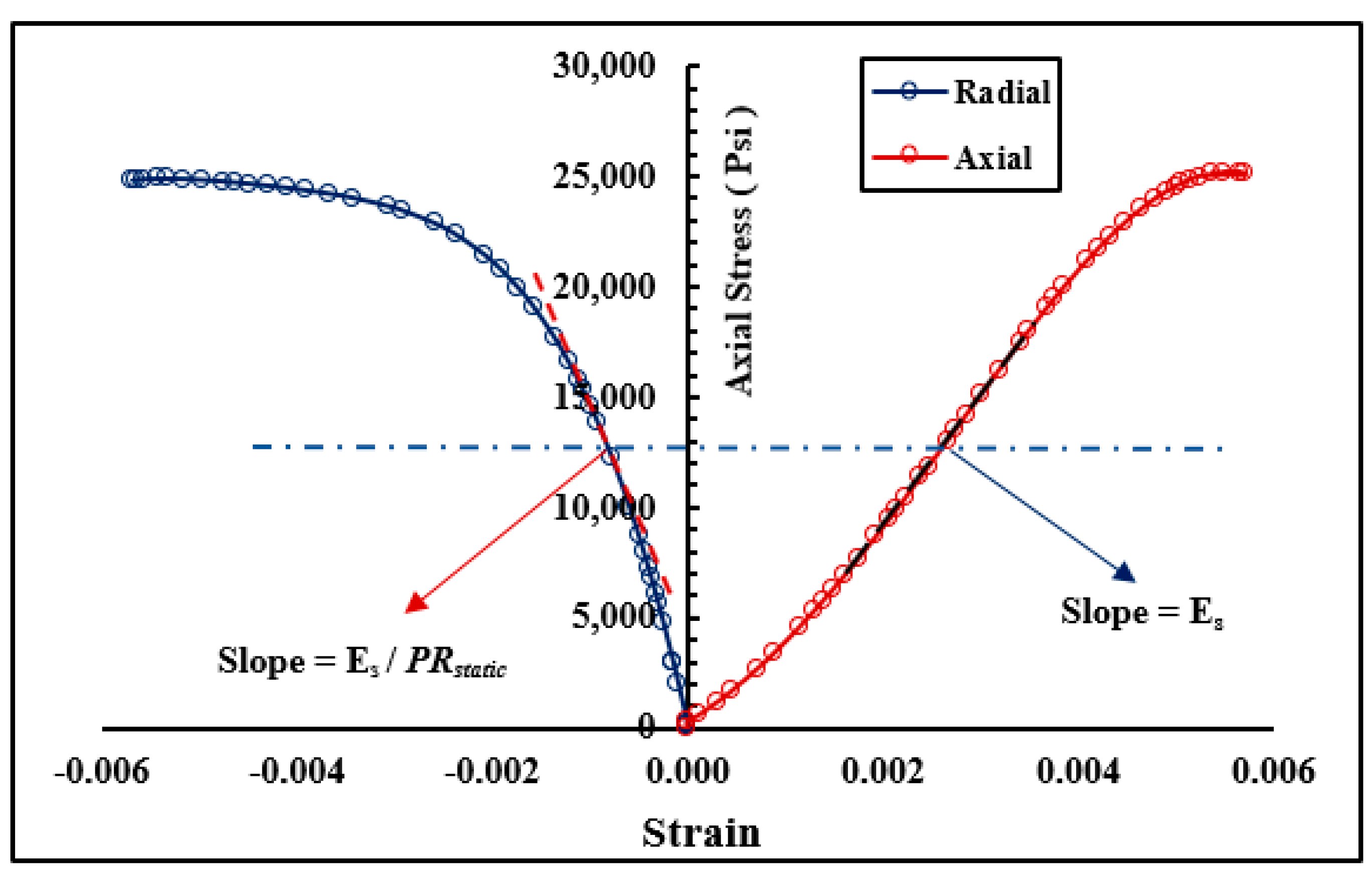
After retrieving core samples representing sandstone sections from the drilled wells, static mechanical properties of the core samples were experimentally determined. These properties (ES and PRstatic) were determined using triaxial compressional tests. Triaxial tests were performed under room temperature and an increasing applied confining pressure from 500 to 1500 psi. The triaxial compression test was conducted according to the recommended practice of the American Society of Testing and Materials (ASTM D 2664-86, ASTM D 3148-93) [31]. Figure 1 shows a stress–strain curve for a retrieved sandstone sample using the triaxial compression test. The values of ES and PRstatic were determined by drawing a tangent straight-line at 50% of the maximum stress value (y-axis) and calculating the slope of this straight line. The slope of the straight-line tangent of the axial stress-strain curve (on the right section) is used to determine ES and the slope of the straight-line tangent of the radial stress-strain curve (on the left section) is used to determine PRstatic.
2.2. Quality Check and Data Filtration
The higher the quality of the training data is, the better the accuracy of AI models [32]. This can be accomplished using technical and statistical approaches. First, any unrealistic values such as negative values and zero values were filtered from the data using MATLAB. Then the quality of the obtained data using the values of P-wave and S-wave velocities was checked by calculating PRdynaimc values using Equation (1). The values of P-wave and S-wave velocities are the reciprocals of and respectively. For typical rocks Poisson’s ratio has positive values; thereafter, any data points yielding negative values of PRdynaimc should be removed [30,32]. Subsequently, any outlier values which significantly deviated from the normal trend were removed. The outliers were removed using a box and whisker plot, in which top whisker represents the upper limit of the data and the bottom whisker represents the lower limit of the data. Any value beyond these limits was considered an outlier and removed [33]. These limits are determined by dividing the data into four equal divisions (quartiles) using the minimum, maximum, mean, and median parameters [34] obtained from the results of statistical analysis of the data listed in Table 1.
2.3. Correction for the Depth Shifting Between Wireline-Logged Depth and Core Depth
The depth of the wireline-logged data are usually measured depending on the length of the wireline used during the logging operation while the recorded depths of core data are based on the length of the drill string. Therefore, it is common to have some mismatch between core and log data. The main reasons for this discrepancy between the two depths are drill pipe stretch, cable stretch, tidal changes, incomplete core recovery, and core expansion [35]. Hence, this difference should be accounted while correlating log data with core measurements. To identify this shift, density-log data are plotted in the same plot with density-data obtained from the core obtained from the same interval [36]. Then, both data are correlated by taking the shift-correction value into account using Equation (3).
2.4. Inputs/Output Relative Importance
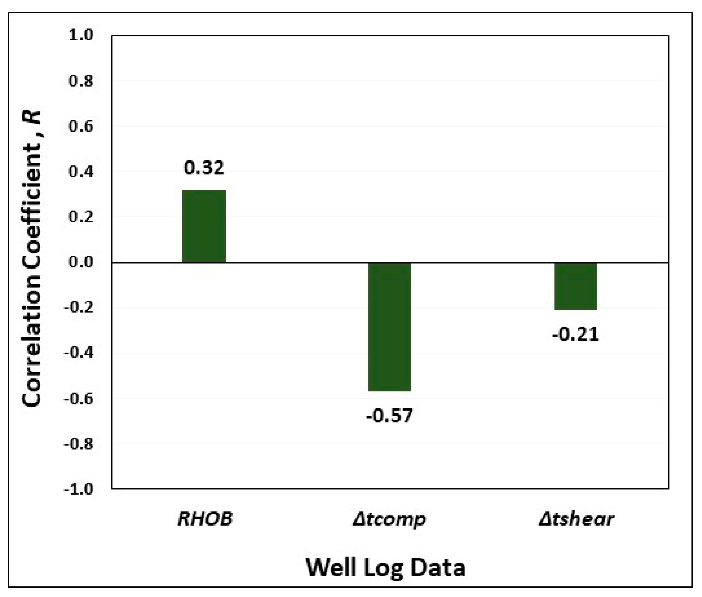
The accuracy of prediction using artificial intelligence (AI) techniques depends on the selected input parameters and their effect on the predicted output. The relative importance of these input parameters with respect to the output can be indicated in terms of the correlation coefficient (R) between them. The correlation coefficient (R) is bounded between −1 and 1. When R equals one, it indicates that the two selected variables are strongly and directly dependent on each other, while for R equals −1, it indicates that they are inversely dependent on each other. When R equals to zero, a linear relationship between these variables does not exist [37]. The mathematical formula used to calculate R is given in Appendix A. Studying the relative importance of the input parameters (RHOB, and ) with the output (PRstatic) resulted in reasonable R values of 0.32, −0.57, −0.21 between PRstatic and the inputs RHOB, , and respectively, as shown in Figure 2.
2.5. The Proposed Prediction Approach
Both artificial neural network (ANN) and self-adaptive differential evolution (SADE) algorithm are implemented in this study to predict PRstatic.
2.5.1. Artificial Neural Network (ANN)
Artificial intelligence (AI) and machine learning have become very effective tools for handling complex engineering problems with high accuracy. Many studies have been reported for utilizing AI tools in rock characterization [38,39,40,41,42,43,44]. Among these tools, ANN is considered one of the most effective and applicable AI techniques, especially in the petroleum industry [45]. Based on the literature, there are many applications of ANN in the field of formation evaluation, such as mechanical property prediction of carbonate rocks [5,21], and reservoir characterization [19,46]. ANN can characterize a system under analysis without the need for any physical phenomenon [47]. There is a significant similarity between the performance of biological neural networks and ANN in processing the input signals to get output responses [48]. The ANN elementary units are called neurons. The minimum number of layers composing the ANN architecture is three; namely input layer, hidden layer, and output layer. These layers are linked using transfer functions and trained using appropriate algorithms representing the nature of the problem [47]. The connections between the neurons are associated with weights and biases [49]. The output layer is commonly assigned to the activation function ‘‘pure linear”, while there are many available options for the transfer functions assigned to input/hidden layers, such as the log-sigmoidal and tan-sigmoidal types [50]. The backpropagation feedforward neural network is recommended as an effective tool in preference to multilayer perceptron (MLP) [15,51]. The number of neurons should be optimized as a large number of neurons may cause over-fitting and negatively affect the prediction process, while using few neurons may yield under-fitting [52].
2.5.2. The Self-Adaptive Differential Evolution (SADE) Algorithm
Differential evolution (DE) is a population-based search technique introduced by Storn and Price [53]. The technique is an outstanding tool used to handle stochastic global optimization problems, which requires tuning and varying a few parameters to get the optimized results. The governing parameters of DE depend significantly on the nature of the problem to be optimized. However, the optimization process, in which the controlling parameters are tuned using different strategies, is excessively time consuming, making the technique computationally expensive [54]. Qin and Suganthan [55] developed the self-adaptive differential evolution (SADE) technique to overcome this drawback. SADE is capable of self-adapting the controlling parameters in a much shorter time compared to DE. SADE is also superior to other optimization algorithms such as particle swarm optimization (PSO), especially for solving numerical problems with medium dimensions [56]. Detailed information on the workflow and the mathematical formulations used in this algorithm have been obtained by many researchers [54,55,57]. SADE has been successfully implemented in many application in the petroleum industry, such as oil production optimization [58] and prediction of spud mud rheology [59].
2.5.3. Building and Implementing of ANN to Predict PRstatic Values
In this study, a new ANN model is developed then optimized using SADE to get the best predictions with the highest possible accuracy. Using such hybrid system increases the performance of the developed network, as indicated in the reviewed studies. The developed approach with the learning algorithm is applied using MATLAB. At first, data are used to train the network and then the results are tested. The evaluation of the network performance in this study depends on the accuracy degree between the actual and the predicted results in terms of three main factors:
- Correlation coefficient (R)
- Mean absolute percentage error (MAPE)
- Coefficient of determination (R2)
The formulas used for R, MAPE, and R2 are listed in Appendix A. MAPE and R2 are considered the most commonly measures used for evaluating the prediction accuracy. More details on MAPE and R2 can be found in [60].
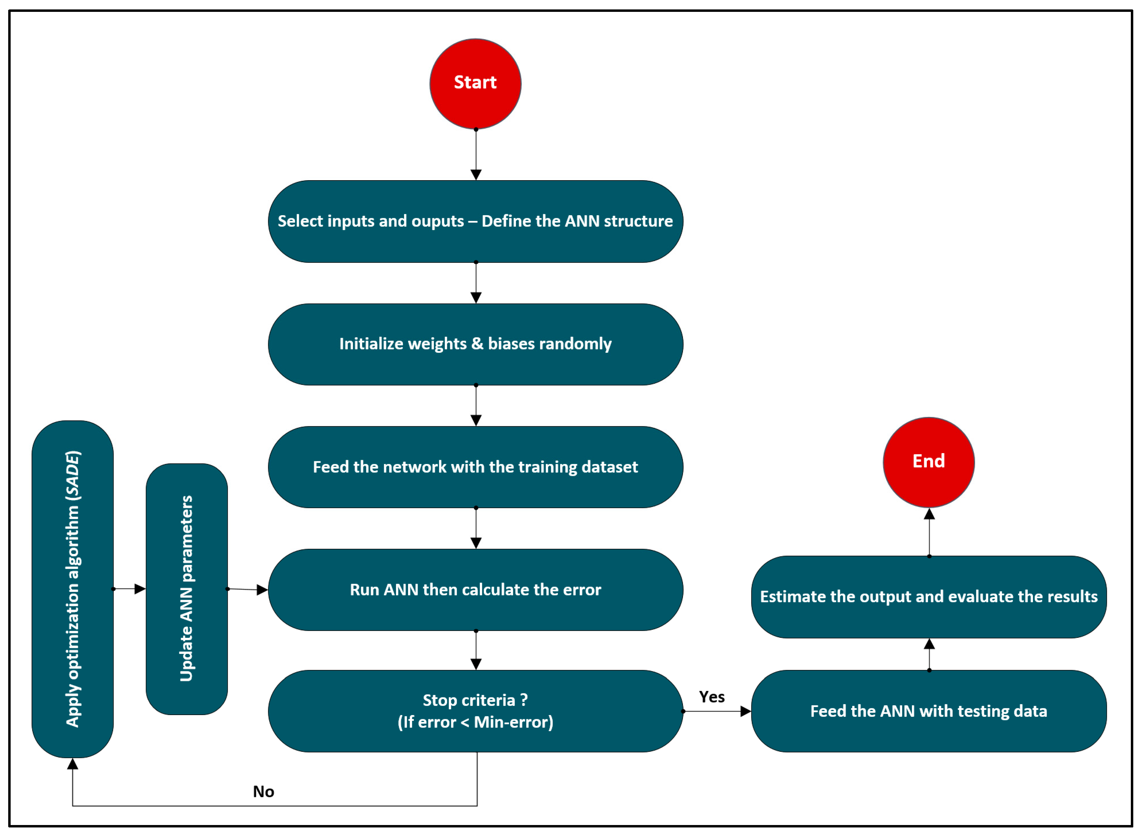
The dataset, including input and output parameters, is used to train the network. Then the network parameters are randomly selected to an optimum choice through iterations. Once the learning algorithm is converged, the determined weights and biases are used to estimate the results using feed forward network structure (FFN) with back propagation learning. This structure contains three layers (input, hidden, and output layers). The number of neurons in the hidden layer are usually estimated using a trial and error technique based on the nature of the problem. The input data are processed through the neurons and their assigned weights and biases; then, the selected transfer function between input/hidden layers is applied to get the response of the hidden layer. Thereafter, the transfer function between hidden/output layers is applied to get the desired output. The network performance is tested based on the results accuracy. Afterwards the error is estimated and propagated back (using back propagation learning) to the earlier layers and SADE is applied to optimize the network parameters based on the obtained results to get more precise results. A simplified flowchart for the developed hybrid approach is shown in Figure 3.
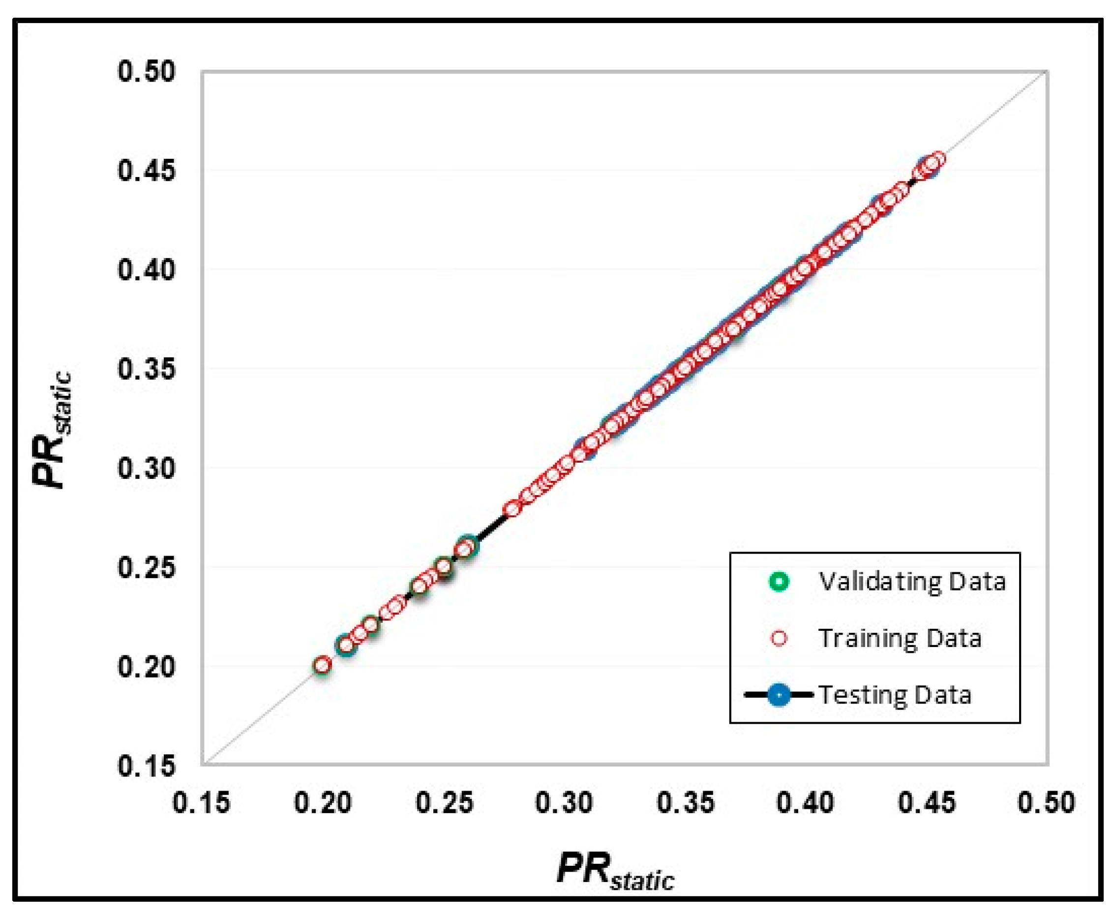
The dataset used for building the ANN model was obtained from drilled wells in the Middle East Region. This set comprises 692 data points representing core data and their corresponding wire-lined log data measurements was used to build the ANN model to estimate the static Poisson’s ratio for sandstone formations. In this study, The ANN model was trained using log data, namely RHOB, , and as input parameters to predict PRstatic. The collected data were randomly divided using MATLAB into two partitions. In total, 631 data points, representing 90% of the selected dataset, were used for training the proposed model and 10% of the dataset (61 data points) was used for testing the model. The dataset was divided in the way that testing data points are within the range of the training data as shown in Figure 4. The input parameters should be fed to the ANN model in the following order: RHOB, , and then . The varying ANN parameters in the optimization process are the number of neurons in the hidden layers, learning rate, training algorithms, number of hidden layers, and transfer functions. Several options of these parameters are used to optimize the model. The optimization process involves tracking the error in the predicted results during training, testing processes through runs of the model for different scenarios. For each scenario, different combinations of these varying parameters are selected and used to train the network. The developed ANN model was optimized using the SADE algorithm, which was described earlier to identify the optimized choices of these parameters which result in the most accurate results. Thereafter, the ANN parameters yielding the lowest possible error in the predicted results are selected as the optimized values. The tested options of ANN parameters are listed in Table 2.
3. Results and Discussion
3.1. Sensitivity Analysis
The SADE-based approach starts initially with a randomly selected population from the obtained dataset. Then, they are processed using an objective function moving through several trials and error by implementing different sets of the aforementioned ANN parameters till reaching the termination criterion of the minimum possible error. Thereafter, ANN is continued with the optimized choices obtained by SADE.
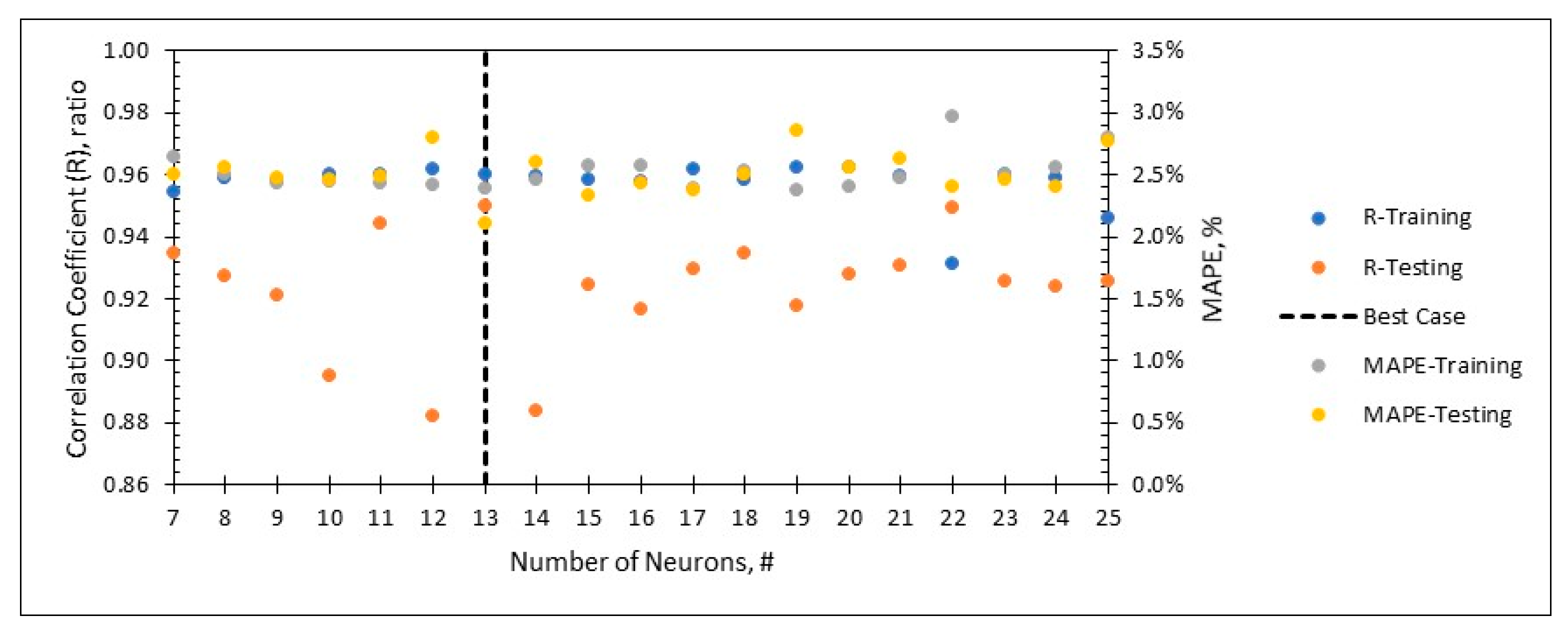
In this study, 20 independent runs are applied to develop the best ANN model in terms of highest R and lowest MAPE between the predicted and actual values. Figure 5 shows the sensitivity of ANN to the varying number of neurons in the hidden layer. The four performance indicators considered in this case are R and MAPE for both the training and testing datasets. The figure demonstrates that 13 neurons leads to the best fit as it could be shown from the highest values of R of 0.96 and 0.95 for training and testing, respectively, as well as the lowest values of MAPE of 2.4 and 2.1% for training and testing, respectively. The figure shows that although different configurations of ANN lead to almost similar fitness results on the training dataset, there is a significant variance on the testing dataset. This confirms the importance of validating ANN on unseen testing dataset to compare the different ANN models.
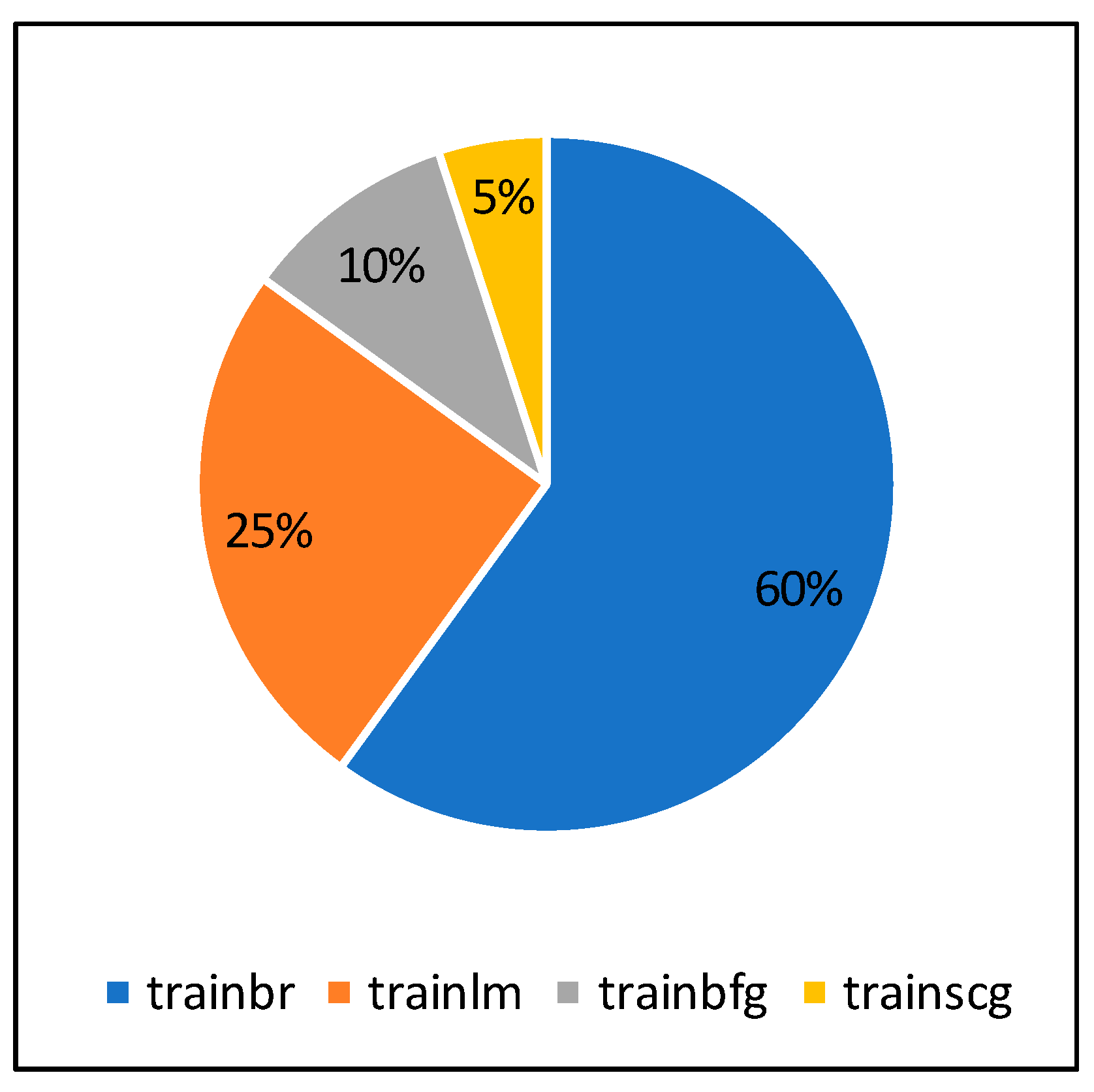
Another governing parameter is the learning algorithm. The Bayesian regularization backpropagation training algorithm (trainbr) shows the best performance as a training function for the developed ANN. Out of 20 independent runs, the performance of the trainbr was superior compared to other training functions in 60% of the runs as shown in Figure 6. This outperformance is due to the fact that that unlike other training functions, the trainbr minimizes a combination of squared errors and weights, and then it identifies the best combination in order to produce an ANN that is able to generalize better (prevent overfitting) than other algorithms. This also can be demonstrated by the high testing R achieved by trainbr, as shown in Figure 7.
3.2. Optimization Process Findings
Consequently, the optimized network would use certain parameters, summarized as follows:
- Only one hidden layer with 13 neurons
- A Bayesian regularization backpropagation (trainbr) training algorithm
- An optimized learning rate of 0.12
- An input/hidden layer transfer function that is Elliot symmetric sigmoid (elliotsig)
- A hidden/output layer transfer function that is pure-linear
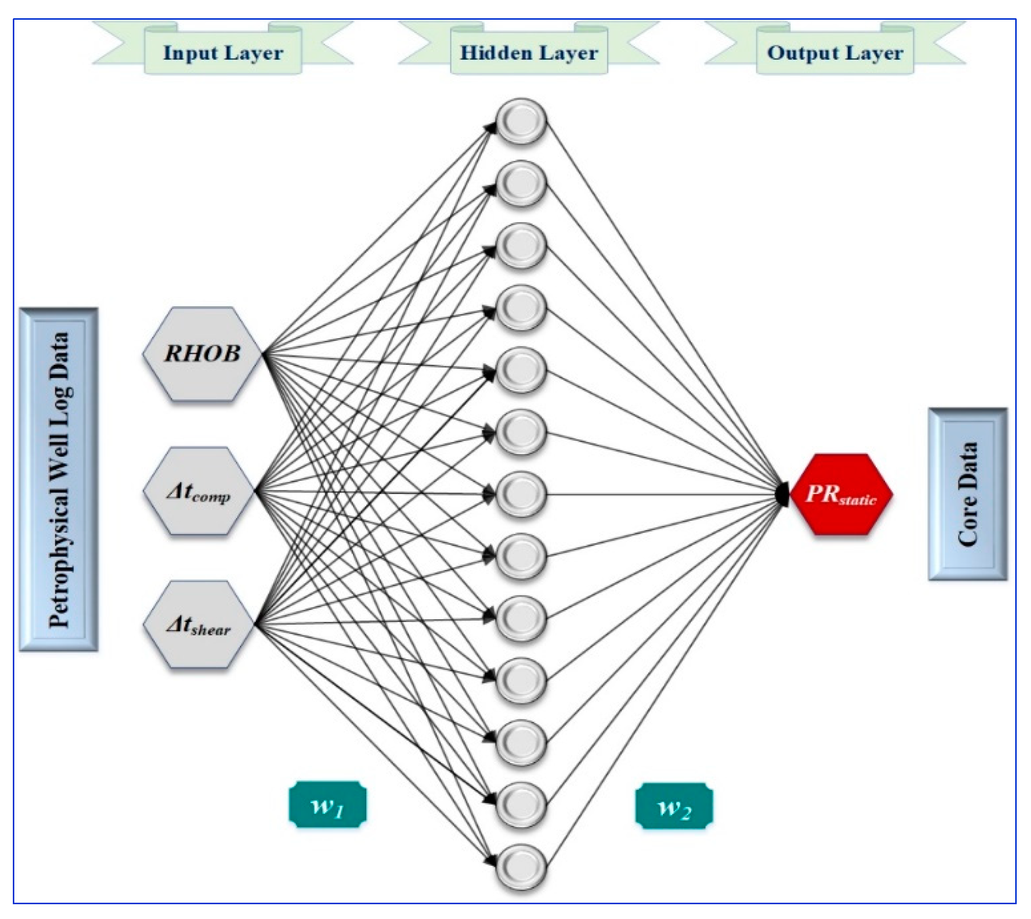
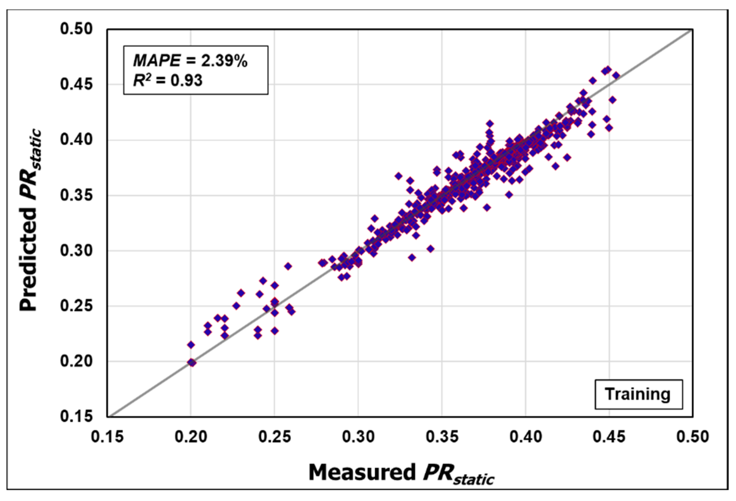
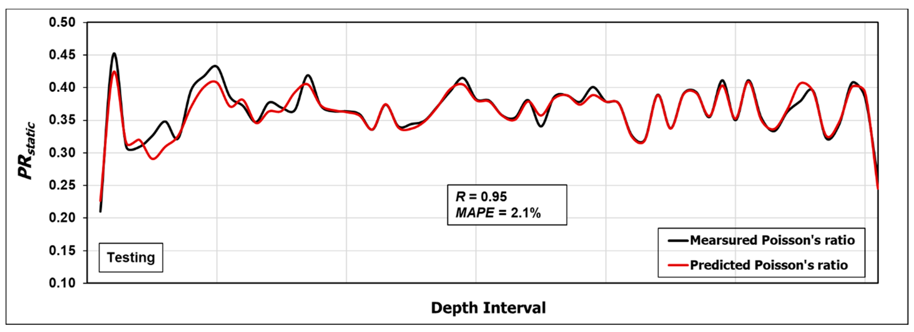
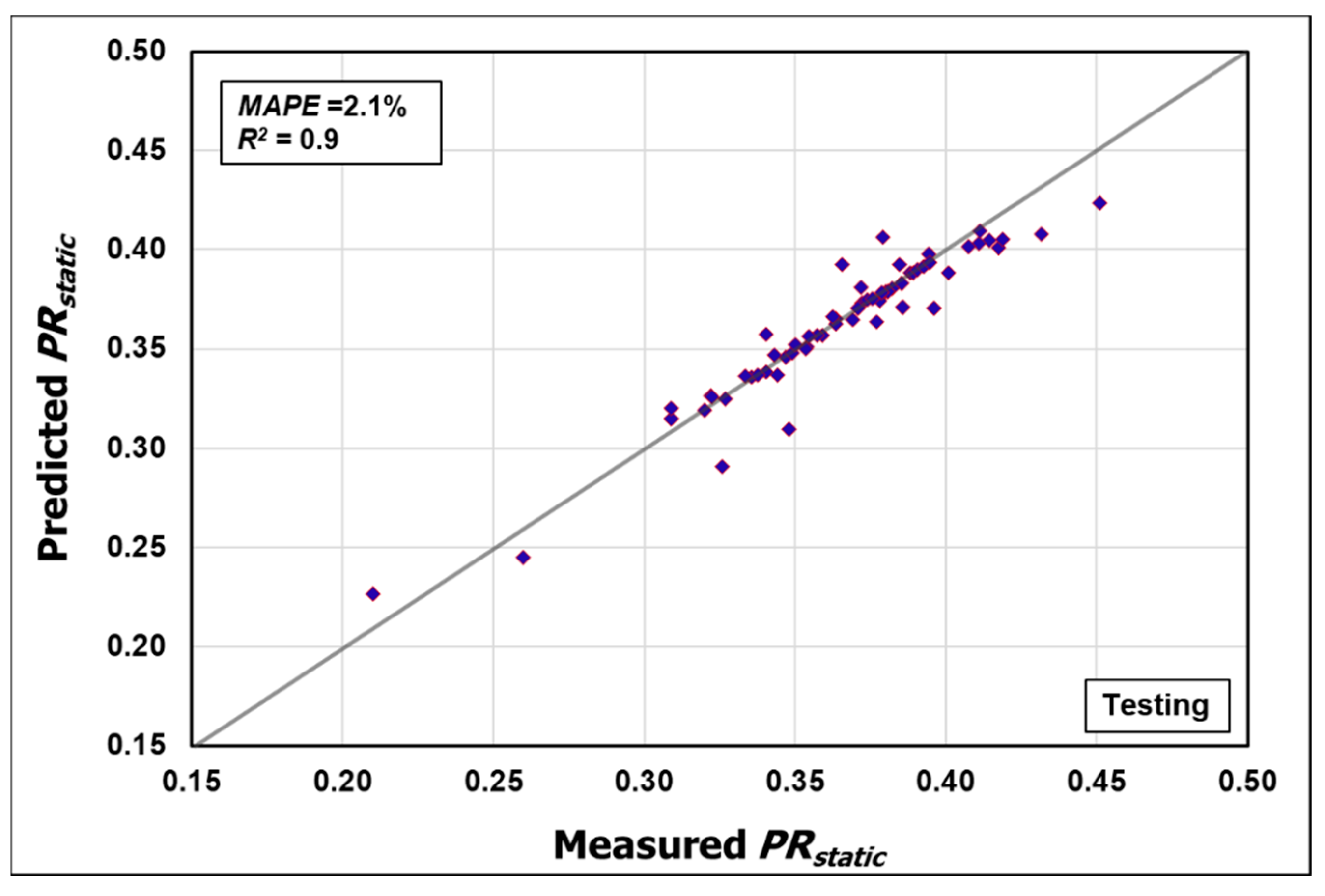
Figure 8 shows a schematic diagram of the architecture of the developed ANN model used to estimate the PRstatic values for sandstone formations. The results obtained from the developed ANN model show a significant match between the measured and predicted PRstatic values from the ANN model. This is indicated by high values of R of 0.96 and MAPE of 2.39% between the measured and predicted PRstatic values for the training process as shown in Figure 9 and Figure 10. Also, the results showed R of 0.95 and MAPE of 2.10% between the measured and predicted PRstatic values for the testing process as depicted in Figure 11 and Figure 12. These findings are only guaranteed if the new input data are within the same range of the dataset used to train the network in order to get accurate predictions of PRstatic, otherwise a large error may be encountered. If the new data are out of that range, the network should be re-trained from the beginning to be updated and to get the new optimized parameters for the new dataset.
3.3. Development of an ANN-Based Mathematical Model
The developed ANN model can be mathematically expressed by Equation (4), which includes the linking weights and biases of the aforementioned three layers of the ANN model (input layer, hidden layer, and output layer).
where PRstatic,n is the normalized value, N is the optimized number of neurons in the hidden layer (n = 13), i is the index of each neuron in the hidden layer, is a matrix of weights linking the input and hidden layers, is a vector of biases linking the input and hidden layers, is a matrix of the weight linking the hidden and output layers, is a bias (scalar) between the hidden and output layers (), represents the weight (associated with neuron of index () in the hidden layer) which will be multiplied by the normalized value of the first input (RHOBn), represents the weight (associated with neuron of index () in the hidden layer) which will be multiplied by the normalized value of the second input (), and represents the weight (associated with neuron of index () in the hidden layer) which will be multiplied by the normalized value of the third input ().
The development of this empirical equation converts the developed ANN model from a black-box mode into a white-box mode. This provides the ability to predict PRstatic values for sandstone formations using Equation (4) by only substituting the required input parameters (RHOB, , ) and the optimized weights and biases listed in Table 3, without the need to run the ANN model. Hence, the feasibility of practical implementation of the developed ANN model is high.
3.4. Procedure to Use the Developed Empirical Equation to Predict PRstatic Values
The developed empirical equation can be used to estimate PRstatic values for sandstone formations according to the steps described below.
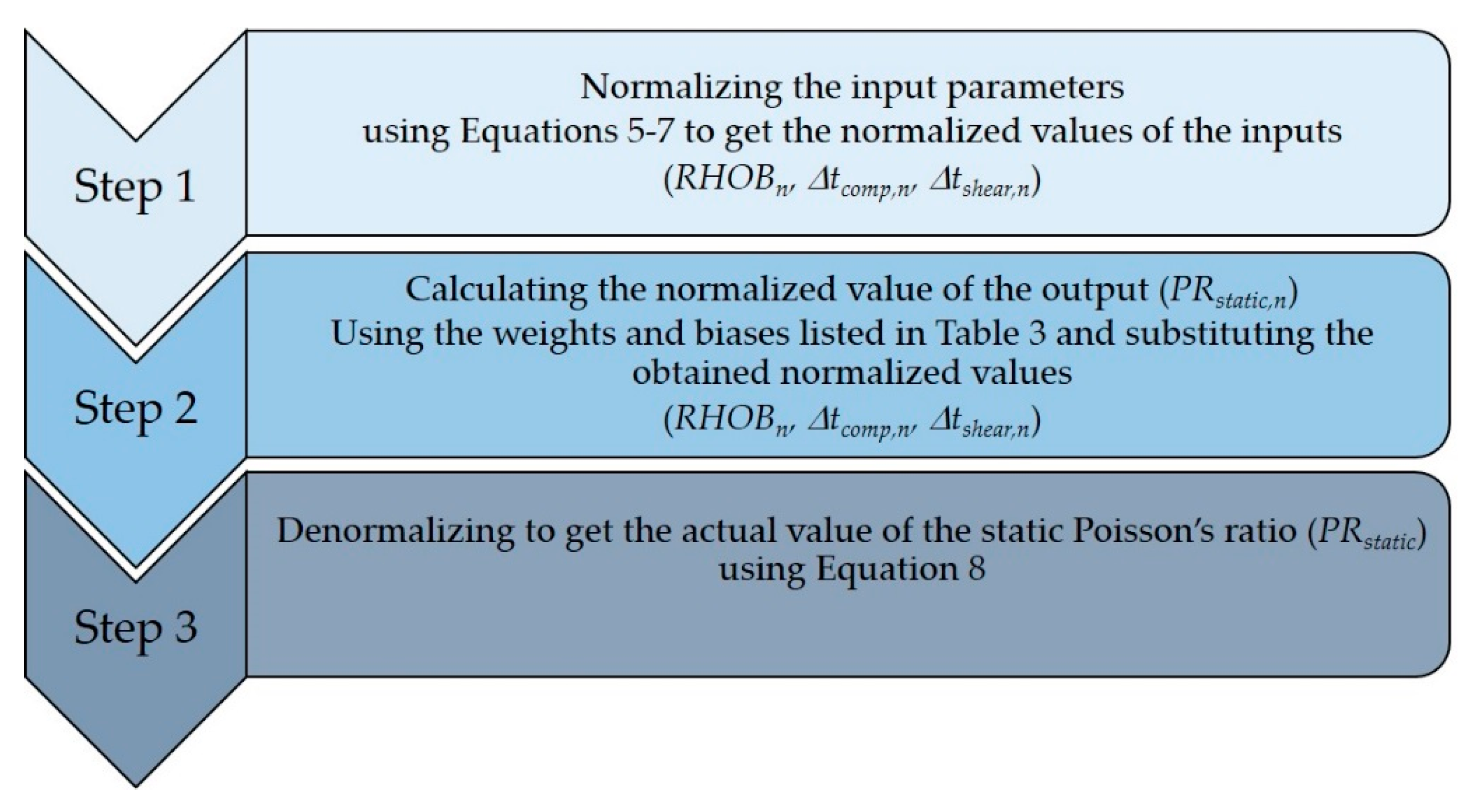
First, the input parameters (RHOB, and ) should be normalized using Equations (5)–(7). The normalized values (RHOBn, and ) are substituted in Equation (4) to calculate the normalized value of the static Poisson’s ratio (PRstatic,n) with the optimized weights and biases listed in Table 3.
Then, the actual value of the static Poisson’s ratio (PRstatic) can be obtained by denormalizing its normalized value (PRstatic,n) using Equation (8). Figure 13 shows a summary of the procedure needed for applying the developed correlation.
3.5. Validation of the Developed ANN Model and the Extracted Equation
The validation process of the developed ANN model is conducted in two main phases:
- Phase 1:
- includes using unseen data from other drilled wells within the same area to predict PRstatic and comparing the results with the actual values.
- Phase 2:
- validates the developed model vs. common previous approaches.
3.5.1. Phase: Validation Using Field Data
For validating the developed ANN model, actual field data from two other wells are used. These data are not included in building the ANN model (training and testing).
Case Number 1
The data collected from well number 1 comprise a continuous profile of petrophysical log data including RHOB, , and measurements of an interval of 550 ft of the sandstone formation, in addition to five core data points representing core samples of the formation within this interval. The log data of these three parameters were used as the inputs to estimate PRstatic using the ANN-based empirical equation expressed in Equation (4). Then, the results obtained from the ANN model are compared with the laboratory measured PRstatic core data. Figure 14 shows that the model estimates PRstatic values within this 550 ft-interval with good match, indicated by R of 0.93 and an MAPE of 4.2% between the predicted and the actual values.
Case Number 2
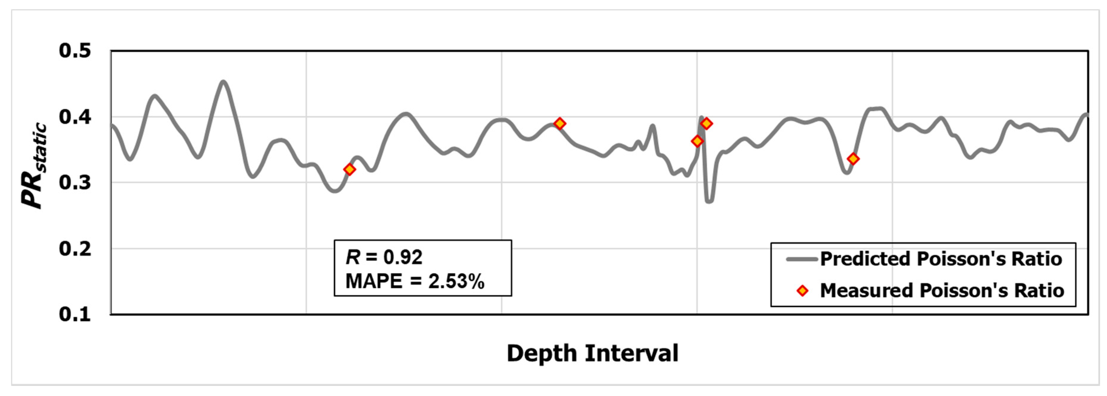
For this well, wire-lined log data (RHOB, , and ) for an interval of 300 ft of sandstone formation are used as inputs. In addition, five experimentally measured core data points of PRstatic are available from the same interval to compare with the results obtained from the ANN model. Figure 15 shows very good agreement between the values measured in the laboratory and predicted PRstatic values, with R of 0.92 and an MAPE of 2.53% between the predicted and the actual values.
3.5.2. Phase 2: Validation by Comparing the Predictions of the ANN Model with Common Previous Approaches
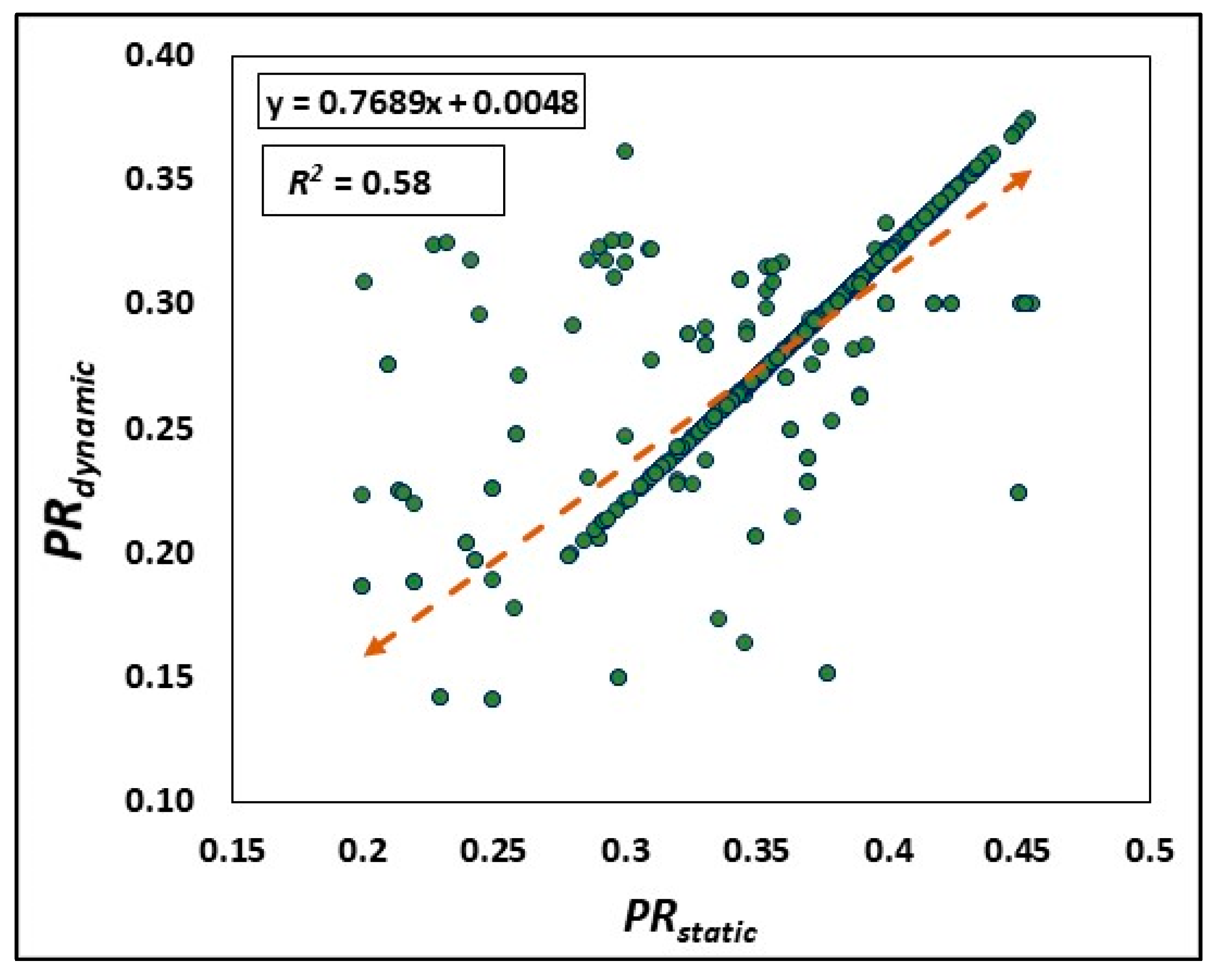
As mentioned before the most reliable measurements of PRstatic values are provided by the lab measurements of core samples representing the desired interval. However, due to the difficulty and complexity to get samples for the depth interval of interest, it is common in the oil and gas industry to use correlations to predict PRstatic values via a standard workflow. These correlations are normally obtained by relating the PRstatic values measured in the laboratory to the calculated PRdynamic from well logs. The dynamic Poisson’s ratio values can be estimated using Vp and Vs via Equation (1). Then PRstatic values can be related to PRdynamic values by plotting PRstatic vs. PRdynamic. In this study, the correlation between the actual PRstatic and the calculated PRdynamic is developed using the same dataset used for building the ANN model resulting in Equation (9) which relates PRstatic with PRdynamic. Thereafter this correlation can be then used to predict PRstatic for other datasets.
Equations (9) is determined by identifying the best fit equation when plotting PRstatic vs. PRdynamic, as shown in Figure 16. The extracted equation shows low coefficient of determination (R2) between PRstatic and PRdynamic of 0.58.
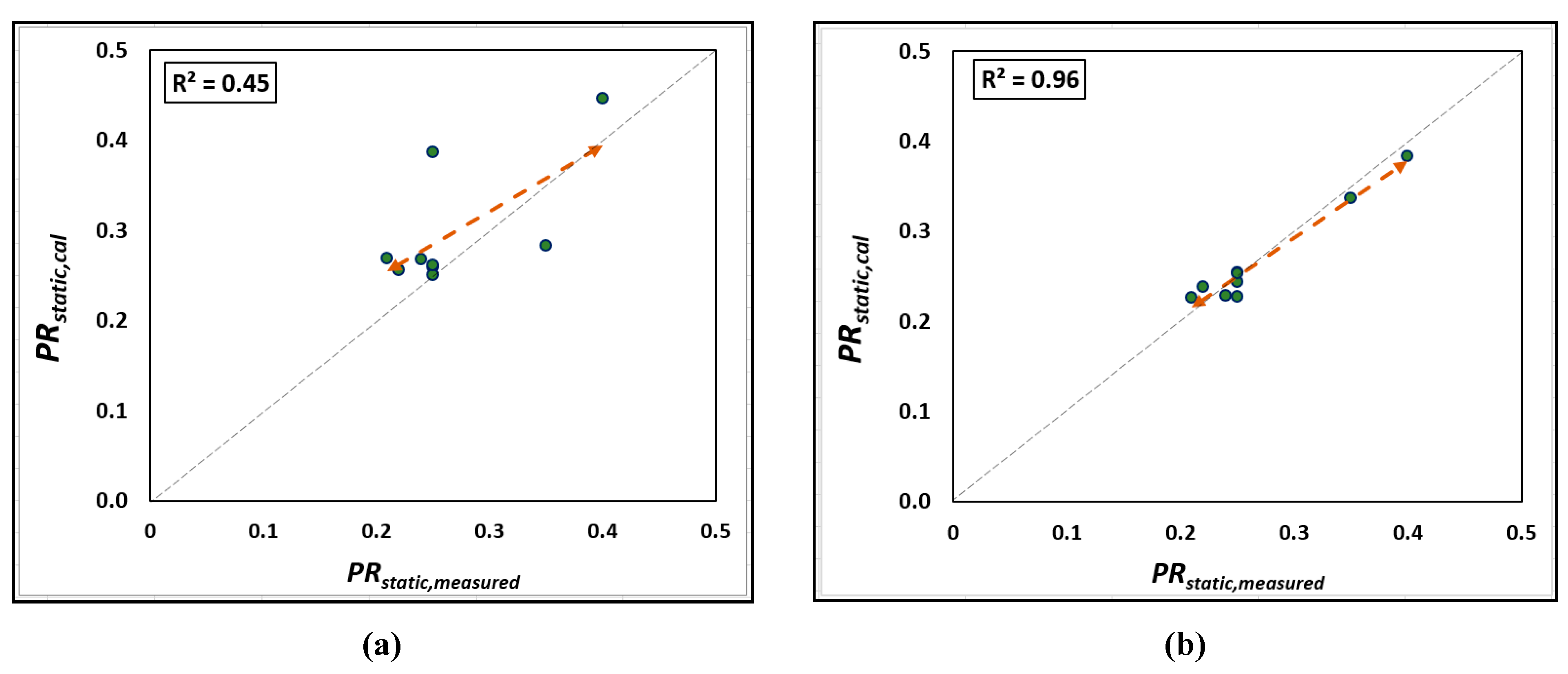
After that another (unseen) dataset representing sandstone sections within the same area is then used to estimate PRstatic using the developed ANN model and Equation (9) and compare the accuracy of the results relative to the actual PRstatic values. Figure 17a,b show comparison between the actual PRstatic and those estimated using the developed ANN model and Equation (9). The developed ANN is found to outperform with R2 of 0.96 compared to R2 of 0.5 using Equation (9). More details about this standard workflow to predict PRstatic can be found in [61,62,63].
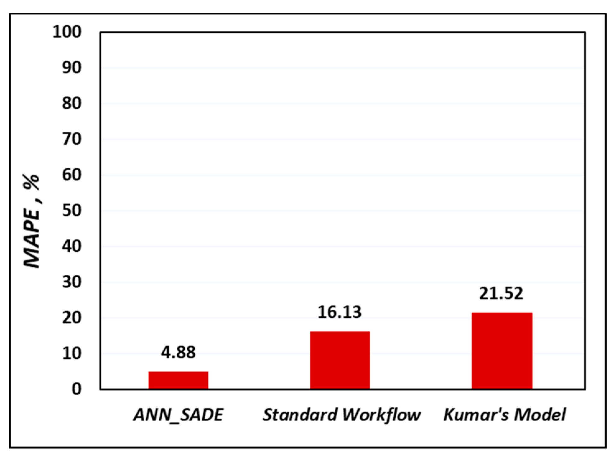
For further confirmation on the superiority of the developed ANN model to predict PRstatic, it is compared with the model developed by Kumar [25]. Kumar developed a correlation relating PRstatic with Vp and Vs stated in Equation (2). Then, PRstatic values are estimated using Kumar’s model (using the same dataset used for validating the ANN model vs. the aforementioned standard workflow) and the results are compared to actual PRstatic values. The performance of the developed ANN model, the standard workflow, and Kumar’s model is evaluated in terms of R, MAPE, and R2 between the estimated and measured PRstatic values, as listed in Table 4 and shown in Figure 18.
4. Conclusions
The self-adaptive differential evolution (SADE) algorithm was implemented to determine the best combination of ANN parameters to predict the static Poisson’s ratio with a high accuracy. Comparing the results obtained from the developed ANN model with the PRstatic values measured in the laboratory demonstrates the following:
- The developed ANN model has the leading predictive efficiency for the static Poisson’s ratio compared with other approaches.
- Petrophysical log data, namely RHOB, , and are used as input parameters for the developed model to produce a continuous profile of PRstatic values whenever these log data are available.
- The extracted ANN-based empirical equation makes the implementation of the developed ANN model easier and more practical, without the need to run the ANN model using any software.
- The developed ANN model allows the estimation of PRstatic values of retrieved sandstone samples without destroying them, which makes them available for more tests.
- The developed ANN-based equation is considered a timely and economically effective tool to estimate PRstatic values, especially when core data are not available.
Author Contributions
Conceptualization, S.E., A.A. and T.M.; methodology, T.M., A.G.; software, T.M.; validation, S.E., A.G. and A.A.; formal analysis, S.E. A.G.; investigation, A.A.; resources, S.E.; data curation, S.E., A.A.; writing—original draft preparation, A.G.; writing—review and editing, A.A., S.E.; visualization, T.M., A.A.; supervision, S.E.
Funding
This research received no external funding.
Acknowledgments
The authors wish to acknowledge King Fahd University of Petroleum and Minerals (KFUPM) for use of various facilities in carrying out this research. Many thanks are due to the anonymous referees for their detailed and helpful comments.
Conflicts of Interest
The author declares no conflict of interest.
Nomenclature
| AI | Artificial intelligence |
| MAPE | Mean absolute percentage error |
| UCS | Unconfined compressive strength |
| ANN | Artificial neural network |
| SADE | self-adaptive differential evolution |
| Tansig | Hyperbolic tangent sigmoid transfer function |
| Hardlim | Hard-limit transfer function |
| Logsig | Log-sigmoid transfer function |
| Pure-linear | Linear transfer function |
| Elliotsig | Elliot symmetric sigmoid transfer function |
| Tribas | Triangular basis transfer function |
| Satlin | Saturating linear transfer function |
| Radbas | Radial basis transfer function |
| Trainlm | Levenberg–Marquardt backpropagation |
| Trainbfg | BFGS quasi-Newton |
| Trainbr | Bayesian regularization backpropagation |
| Trainscg | Scaled conjugate gradient backpropagation |
| List of Symbols | |
| R2 | Coefficient of determination |
| PRstatic | Static Poisson’s ratio |
| PRdynamic | Dynamic Poisson’s ratio |
| RHOB | Formation bulk density |
| P-wave | Compressional wave |
| S-wave | Shear wave |
| P-wave transit time | |
| S-wave transit time | |
| T | Tensile strength |
| Overburden stress | |
| Horizontal stress | |
| Vp | P-wave velocity |
| Vs | S-wave velocity |
| Es | Static Young’s modulus |
| b1 | Input layer biases |
| b2 | Output layer bias |
| N | Number of neurons in the hidden layer |
| R | Correlation coefficient |
| w1 | Weights linking inputs and hidden layer |
| w2 | Weights linking output and hidden layer |
| Subscripts | |
| i | Index of each neuron in the hidden layer |
| n | Normalized value |
Appendix A
The formula of correlation coefficient (R) between any two variables (x, y) used in this study is expressed as:
where K is the number of dataset points.
Mean absolute percentage error (MAPE) is expressed as:
where m is the number of dataset points.
Coefficient of determination (R2)
References
- Anifowose, F.; Adeniye, S.; Abdulraheem, A.; Al-Shuhail, A. Integrating seismic and log data for improved petroleum reservoir properties estimation using non-linear feature-selection based hybrid computational intelligence models. J. Pet. Sci. Eng. 2016, 145, 230–237. [Google Scholar] [CrossRef]
- Anifowose, F.A.; Labadin, J.; Abdulraheem, A. Ensemble model of non-linear feature selection-based extreme learning machine for improved natural gas reservoir characterization. J. Nat. Gas Sci. Eng. 2015, 26, 1561–1572. [Google Scholar] [CrossRef]
- Helmy, T.; Hossain, M.I.; Adbulraheem, A.; Rahman, S.M.; Hassan, M.R.; Khoukhi, A.; Elshafei, M. Prediction of non-hydrocarbon gas components in separator by using hybrid computational intelligence models. Neural Comput. Appl. 2017, 28, 635–649. [Google Scholar] [CrossRef]
- Al-Bulushi, N.I.; King, P.R.; Blunt, M.J.; Kraaijveld, M. Artificial neural networks workflow and its application in the petroleum industry. Neural Comput. Appl. 2012, 21, 409–421. [Google Scholar] [CrossRef]
- Tariq, Z.; Elkatatny, S.; Mahmoud, M.; Ali, A.Z.; Abdulraheem, A. A new technique to develop rock strength correlation using artificial intelligence tools. In SPE Reservoir Characterisation and Simulation Conference and Exhibition; Society of Petroleum Engineers: Calgary, AB, Canada, 2017. [Google Scholar] [CrossRef]
- Nes, O.M.; Fjær, E.; Tronvoll, J.; Kristiansen, T.G.; Horsrud, P. Drilling time reduction through an integrated rock mechanics analysis. In Proceedings of the SPE/IADC Drilling Conference, Amsterdam, The Netherlands, 23–25 February 2005. [Google Scholar]
- Zhang, H.; Qiu, K.; Fuller, J.; Yin, G.; Yuan, F.; Chen, S. Geomechanical Evaluation Enabled Successful Stimulation of a HPHT Tight Gas Reservoir in Western China. In Proceedings of the International Petroleum Technology Conference, Kuala Lumpur, Malaysia, 19–22 January 2014. [Google Scholar]
- Tutuncu, A.N.; Sharma, M.M. Relating Static and Ultrasonic Laboratory Measurements to Acoustic Log Measurements in Tight Gas Sands. In Proceedings of the SPE Annual Technical Conference and Exhibition, Washington, DC, USA, 4–7 October 1992. [Google Scholar] [CrossRef]
- Gatens, J.M., III; Harrison, C.W., III; Lancaster, D.E.; Guidry, F.K. In-situ stress tests and acoustic logs determine mechanical propertries and stress profiles in the devonian shales. SPE Formation Eval. 1990, 5, 248–254. [Google Scholar] [CrossRef]
- Najibi, A.R.; Ghafoori, M.; Lashkaripour, G.R.; Asef, M.R. Empirical relations between strength and static and dynamic elastic properties of Asmari and Sarvak limestones, two main oil reservoirs in Iran. J. Pet. Sci. Eng. 2015, 126, 78–82. [Google Scholar] [CrossRef]
- Tariq, Z.; Mahmoud, M.; Abdulraheem, A. Core log integration: A hybrid intelligent data-driven solution to improve elastic parameter prediction. Neural. Comput. Appl. 2019, 1–21. [Google Scholar] [CrossRef]
- Nawrocki, P.A.; Dusseault, M.B. Modelling of Damaged Zones around Boreholes Using a Radius Dependent Young’s Modulus. J. Can. Pet. Technol. 1996, 35, 31–35. [Google Scholar] [CrossRef]
- Wang, C.; Wu, Y.S.; Xiong, Y.; Winterfeld, P.H.; Huang, Z. Geomechanics coupling simulation of fracture closure and its influence on gas production in shale gas reservoirs. In Proceedings of the SPE Reservoir Simulation Symposium, Houston, TA, USA, 23–25 February 2015. [Google Scholar]
- Ameen, M.S.; Smart, B.G.; Somerville, J.M.; Hammilton, S.; Naji, N.A. Predicting rock mechanical properties of carbonates from wireline logs (a case study: Arab-D reservoir, Ghawar field, Saudi Arabia). Mar. Pet. Geol. 2009, 26, 430–444. [Google Scholar] [CrossRef]
- Elkatatny, S.; Mahmoud, M.; Mohamed, I.; Abdulraheem, A. Development of a new correlation to determine the static Young’s modulus. J. Pet. Explor. Prod. Technol 2018, 8, 17–30. [Google Scholar] [CrossRef]
- Spain, D.R.; Gil, I.R.; Sebastian, H.M.; Smith, P.; Wampler, J.; Cadwallader, S.; Graff, M. Geo-engineered completion optimization: An integrated, multi-disciplinary approach to improve stimulation efficiency in unconventional shale reservoirs. In Proceedings of the SPE Middle East Unconventional Resources Conference and Exhibition, Muscat, Oman, 26–28 January 2015. [Google Scholar]
- Mahmoud, M.; Elkatatny, S.; Ramadan, E.; Abdulraheem, A. Development of lithology-based static Young’s modulus correlations from log data based on data clustering technique. J. Pet. Sci. Eng. 2016, 146, 10–20. [Google Scholar] [CrossRef]
- Tariq, Z.; Elkatatny, S.; Mahmoud, M.; Abdulraheem, A. A new artificial intelligence based empirical correlation to predict sonic travel time. In Proceedings of the International Petroleum Technology Conference, Bangkok, Thailand, 14–16 November 2016. [Google Scholar]
- Tariq, Z.; Elkatatny, S.; Mahmoud, M.; Ali, A.Z.; Abdulraheem, A. A new technique to develop rock strength correlation using artificial intelligence tools. In Proceedings of the SPE Reservoir Characterisation and Simulation Conference and Exhibition, Abu Dhabi, UAE, 8–10 May 2017. [Google Scholar]
- Tariq, Z.; Elkatatny, S.M.; Mahmoud, M.A.; Abdulraheem, A.; Abdelwahab, A.Z.; Woldeamanuel, M. Estimation of Rock Mechanical Parameters Using Artificial Intelligence Tools; American Rock Mechanics Association: San Francisco, CA, USA, 2017. [Google Scholar]
- Elkatatny, S.; Tariq, Z.; Mahmoud, M.; Abdulraheem, A.; Mohamed, I. An integrated approach for estimating static Young’s modulus using artificial intelligence tools. Neural Comput. Appl. 2018. [Google Scholar] [CrossRef]
- D’Andrea, D.V.; Fischer, R.L.; Fogelson, D.E. Prediction of Compressive Strength from Other Rock Properties; US Department of the Interior, Bureau of Mines: Washington, DC, USA, 1965; Volume 6702.
- Kumar, J. The effect of Poisson’s ratio on rock properties. In Proceedings of the SPE Annual Fall Technical Conference and Exhibition, New Orleans, LA, USA, 3–6 October 1976. [Google Scholar]
- Edimann, K.; Somerville, J.M.; Smart, B.G.D.; Hamilton, S.A.; Crawford, B.R. Predicting rock mechanical properties from wireline porosities. In Proceedings of the SPE/ISRM Rock Mechanics in Petroleum Engineering, Trondheim, Norway, 8–10 July 1998. [Google Scholar]
- Kumar, A.; Jayakumar, T.; Raj, B.; Ray, K.K. Correlation between ultrasonic shear wave velocity and Poisson’s ratio for isotropic solid materials. Acta Mater. 2003, 51, 2417–2426. [Google Scholar] [CrossRef]
- Al-Shayea, N.A. Effects of testing methods and conditions on the elastic properties of limestone rock. Eng. Geol. 2004, 74, 139–156. [Google Scholar] [CrossRef]
- Singh, V.; Singh, T.N. A Neuro-Fuzzy Approach for Prediction of Poisson’s Ratio and Young’s Modulus of Shale and Sandstone. In Proceedings of the 41st US Symposium on Rock Mechanics (USRMS), Golden, CO, USA, 17–21 June 2006. [Google Scholar]
- Shalabi, F.I.; Cording, E.J.; Al-Hattamleh, O.H. Estimation of rock engineering properties using hardness tests. Eng. Geol. 2007, 90, 138–147. [Google Scholar] [CrossRef]
- Al-Anazi, A.; Gates, I.D. A support vector machine algorithm to classify lithofacies and model permeability in heterogeneous reservoirs. Eng. Geol. 2010, 114, 267–277. [Google Scholar] [CrossRef]
- Abdulraheem, A. Prediction of Poisson’s Ratio for Carbonate Rocks Using ANN and Fuzzy Logic Type-2 Approaches. In Proceedings of the International Petroleum Technology Conference, Beijing, China, 26 March 2019. [Google Scholar]
- ASTM D2664-04. Standard Test Method for Triaxial Compressive Strength of Undrained Rock Core Specimens without Pore Pressure Measurements. 2005. Available online: https://www.astm.org/Standards/D2664.htm (accessed on 3 April 2019).
- Gercek, H. Poisson’s ratio values for rocks. Int. J. Rock Mech. Min. Sci. 2007, 44, 1–13. [Google Scholar] [CrossRef]
- Dawson, R. How Significant Is A Boxplot Outlier? J. Stat. Educ. 2011, 19. [Google Scholar] [CrossRef]
- Thirumalai, C.S.; Manickam, V.; Balaji, R. Data analysis using Box and Whisker Plot for Lung Cancer. In Proceedings of the 2017 Innovations in Power and Advanced Computing Technologies, Vellore, Tamil Nadu, India, 21–22 April 2017. [Google Scholar] [CrossRef]
- Fontana, E.; Iturrino, G.J.; Tartarotti, P. Depth-shifting and orientation of core data using a core–log integration approach: A case study from ODP–IODP Hole 1256D. Tectonophysics 2010, 494, 85–100. [Google Scholar] [CrossRef]
- Nadezhdin, O.; Zairullina, E.; Efimov, D.; Savichev, V. Algorithms of Automatic Core-Log Depth-Shifting In Problems of Petrophysical Model Construction, Proceedings of the SPE Russian Oil and Gas Exploration & Production Technical Conference and Exhibition; Society of Petroleum Engineers: Moscow, Russia, 16 October 2014. [Google Scholar]
- Benesty, J.; Chen, J.; Huang, Y.; Cohen, I. Pearson correlation coefficient. In Noise Reduction in Speech Processing; Springer: Berlin, Genmany, 2009; pp. 1–4. [Google Scholar]
- Sudakov, O.; Burnaev, E.; Koroteev, D. Driving Digital Rock towards Machine Learning:predicting permeability with Gradient Boosting and Deep Neural Networks. Comput. Geosci. 2018, 127, 91–98. [Google Scholar] [CrossRef]
- Chauhan, S.; Rühaak, W.; Anbergen, H.; Kabdenov, A.; Freise, M.; Wille, T.; Sass, I. Phase segmentation of X-ray computer tomography rock images using machine learning techniques: An accuracy and performance study. Solid Earth 2016, 7, 1125–1139. [Google Scholar] [CrossRef]
- Chauhan, S.; Rühaak, W.; Khan, F.; Enzmann, F.; Mielke, P.; Kersten, M.; Sass, I. Processing of rock core microtomography images: Using seven different machine learning algorithms. Comput. Geosci. 2016, 86, 120–128. [Google Scholar] [CrossRef]
- Tahmasebi, P.; Javadpour, F.; Sahimi, M. Data mining and machine learning for identifying sweet spots in shale reservoirs. Expert Syst. Appl. 2017, 88, 435–447. [Google Scholar] [CrossRef]
- Mousavi Nezhad, M.; Gironacci, E.; Rezania, M.; Khalili, N. Stochastic modelling of crack propagation in materials with random properties using isometric mapping for dimensionality reduction of nonlinear data sets. Int. J. Numer. Methods Eng. 2017, 113, 656–680. [Google Scholar] [CrossRef] [Green Version]
- Keller, L.M.; Schwiedrzik, J.J.; Gasser, P.; Michler, J. Understanding anisotropic mechanical properties of shales at different length scales: In situ micropillar compression combined with finite element calculations. J. Geophys. Res. Solid Earth 2017, 122. [Google Scholar] [CrossRef]
- Sone, H.; Zoback, M.D. Mechanical properties of shale-gas reservoir rocks—Part 1: Static and dynamic elastic properties and anisotropy. Geophysics 2013, 78, 381–392. [Google Scholar] [CrossRef]
- Rable, B. The Future is Here: 3 Ways AI Roots Itself in O&G in the Surge Magazine. 2017. Available online: http://thesurge.com/stories/future-artificial-intelligence-roots-oil-gas-industry (accessed on 3 April 2019).
- Anifowose, F.A.; Labadin, J.; Abdulraheem, A. Ensemble machine learning: An untapped modeling paradigm for petroleum reservoir characterization. J. Pet. Sci. Eng. 2017, 151, 480–487. [Google Scholar] [CrossRef]
- Lippman, R.P. An introduction to computing with neural nets. IEEE ASSP Mag. 1987, 4, 4–22. [Google Scholar] [CrossRef]
- Nakamoto, P. Neural Networks and Deep Learning: Deep Learning Explained to Your Granny a Visual Introduction for Beginners Who Want to Make Their Own Deep Learning Neural Network (Machine Learning); CreateSpace Independent Publishing Platform: Scotts Valley, CA, USA, 2017. [Google Scholar]
- Hinton, G.E.; Osindero, S.; Teh, Y.-W. A fast learning algorithm for deep belief nets. Neural Comput. 2006, 18, 1527–1554. [Google Scholar] [CrossRef]
- Niculescu, S. Artificial neural networks and genetic algorithms in Qsar. J. Mol. Struct. 2003, 622, 71–83. [Google Scholar] [CrossRef]
- Yılmaz, I.; Yuksek, A.G. An example of artificial neural network (ANN) application for indirect estimation of rock parameters. Rock Mech. Rock Eng. 2008, 41, 781–795. [Google Scholar] [CrossRef]
- Rao, S.; Ramamurti, V. A hybrid technique to enhance the performance of recurrent neural networks for time series prediction. In Proceedings of the IEEE international conference on neural networks, San Francisco, CA, USA, 28 March–1 April 1993; pp. 52–57. [Google Scholar]
- Storn, R.; Price, K. Differential Evolution: A Simple and Efficient Adaptive Scheme for Global Optimization Over Continuous Spaces. J. Glob. Optim. 1995, 23, 341–359. [Google Scholar]
- Goudos, S.K.; Baltzis, K.B.; Antoniadis, K.; Zaharis, Z.D.; Hilas, C.S. A comparative study of common and self-adaptive differential evolution strategies on numerical benchmark problems. Procedia Comput. Sci. 2011, 3, 83–88. [Google Scholar] [CrossRef] [Green Version]
- Qin, A.K.; Suganthan, P.N. Self-adaptive differential evolution algorithm for numerical optimization. In Proceedings of the IEEE Congress on Evolutionary Computation, Edinburgh, UK, 2–4 September 2005; Volume 2, pp. 178–1791. [Google Scholar]
- Vesterstrom, J.; Thomsen, R. A comparative study of differential evolution, particle swarm optimization, and evolutionary algorithms on numerical benchmark problems. In Proceedings of the 2004 Congress on Evolutionary Computation, Portland, OR, USA, 19–23 June 2004. [Google Scholar]
- Qin, A.K.; Huang, V.L.; Suganthan, P.N. Differential evolution algorithm with strategy adaptation for global numerical optimization. IEEE Trans. Evol. Comput. 2009, 13, 398–417. [Google Scholar] [CrossRef]
- Foroud, T.; Baradaran, A.; Seifi, A. A comparative evaluation of global search algorithms in black box optimization of oil production: A case study on Brugge field. J. Pet. Sci. Eng. 2018, 167, 131–151. [Google Scholar] [CrossRef]
- Abdelgawad, K.; Elkatatny, S.; Moussa, T.; Mahmoud, M.; Patil, S. Real-Time Determination of Rheological Properties of Spud Drilling Fluids Using a Hybrid Artificial Intelligence Technique. J. Energy Resour. Technol. 2019, 141, 032908. [Google Scholar] [CrossRef]
- Smith, G. Essential Statistics Regression and Econometrics; Academic Press: Cambridge, MA, USA, 2015. [Google Scholar]
- Kim, S.; Kim, H. A new metric of absolute percentage error for intermittent demand forecasts. Int. J. Forecast. 2016, 32, 669–679. [Google Scholar] [CrossRef]
- Yale, D.P. Static and Dynamic Rock Mechanical Properties in the Hugoton and Panoma Fields, Kansas. In Proceedings of the SPE Mid-Continent Gas Symposium, Amarillo, TX, USA, 22–24 May 1994. [Google Scholar]
- Montmayeur, H.; Graves, R.M. Prediction of static elastic/mechanical properties of consolidated and unconsolidated sands from acoustic measurements: Correlations. In Proceedings of the SPE Annual Technical Conference and Exhibition, Houston, TX, USA, 3–6 October 1993. [Google Scholar]
Figure 1.
A typical axial and radial stress–strain curve obtained from the triaxial test of a sandstone sample.
Figure 1.
A typical axial and radial stress–strain curve obtained from the triaxial test of a sandstone sample.

Figure 2.
Relative importance between the input parameters and the output, the static Poisson’s ratio (PRstatic).
Figure 2.
Relative importance between the input parameters and the output, the static Poisson’s ratio (PRstatic).

Figure 3.
Flowchart describing the workflow of the hybrid approach ANN-SADE. ANN: artificial neural network; SADE: self-adaptive differential evolution.
Figure 3.
Flowchart describing the workflow of the hybrid approach ANN-SADE. ANN: artificial neural network; SADE: self-adaptive differential evolution.

Figure 4.
Testing data ranges with respect to the training data used for developing the ANN model.

Figure 5.
Sensitivity analysis of the ANN performance for varying number of neurons.

Figure 6.
Success rate of each of the training functions out of the 20 independent runs.

Figure 7.
Comparison analysis between the tested training functions.

Figure 8.
Schematic diagram of the architecture of the developed ANN model showing the input and output parameters with the optimized number of neurons (13 neurons) and assigned weights and biases between the model layers.
Figure 8.
Schematic diagram of the architecture of the developed ANN model showing the input and output parameters with the optimized number of neurons (13 neurons) and assigned weights and biases between the model layers.

Figure 9.
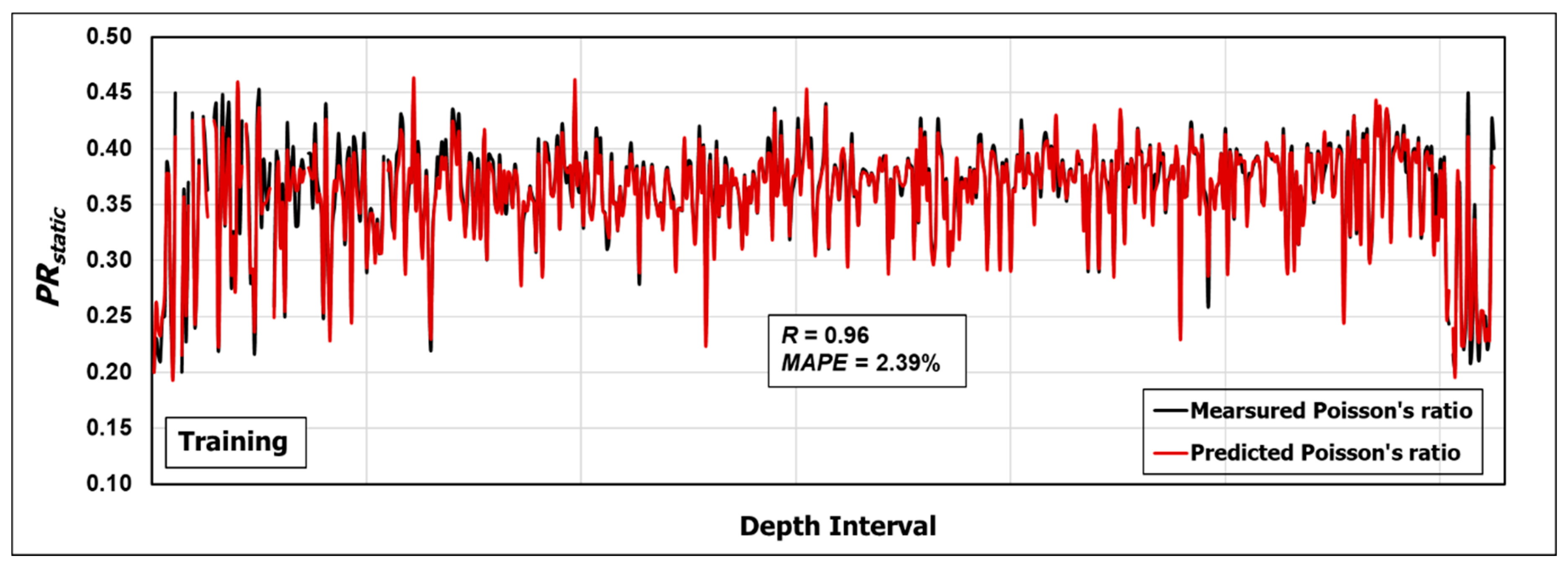
Comparison profile between predicted PRstatic vs. measured PRstatic during the training process showing a high match between the predicted and measured values with a correlation coefficient (R) of 0.96 and mean absolute percentage error (MAPE) of 2.39%.
Figure 9.
Comparison profile between predicted PRstatic vs. measured PRstatic during the training process showing a high match between the predicted and measured values with a correlation coefficient (R) of 0.96 and mean absolute percentage error (MAPE) of 2.39%.

Figure 10.
Cross plot between predicted PRstatic vs. measured PRstatic for the training process with an R2 of 0.9 between the predicted and measured values.
Figure 10.
Cross plot between predicted PRstatic vs. measured PRstatic for the training process with an R2 of 0.9 between the predicted and measured values.

Figure 11.
Comparison profile between predicted PRstatic vs. measured PRstatic during the testing process, showing a significant match between the predicted and measured values with R of 0.95 and MAPE of 2.10%.
Figure 11.
Comparison profile between predicted PRstatic vs. measured PRstatic during the testing process, showing a significant match between the predicted and measured values with R of 0.95 and MAPE of 2.10%.

Figure 12.
Cross plot between predicted PRstatic vs. measured PRstatic for the testing process with R2 of 0.90 between the predicted and measured values.
Figure 12.
Cross plot between predicted PRstatic vs. measured PRstatic for the testing process with R2 of 0.90 between the predicted and measured values.

Figure 13.
Procedure to apply the developed ANN-based correlation.

Figure 14.
Comparison of the predicted PRstatic values by the ANN model with the measured values for cores from well number 1 (R = 0.93, MAPE = 4.2%).
Figure 14.
Comparison of the predicted PRstatic values by the ANN model with the measured values for cores from well number 1 (R = 0.93, MAPE = 4.2%).

Figure 15.
Comparison of the PRstatic values predicted by the ANN model with the measured values for cores from well number 2 (R = 0.92, MAPE = 2.53%).
Figure 15.
Comparison of the PRstatic values predicted by the ANN model with the measured values for cores from well number 2 (R = 0.92, MAPE = 2.53%).

Figure 16.
Relationship between PRstatic vs. PRdynamic using well log data (Vp and Vs) for sandstone sections in the same area.
Figure 16.
Relationship between PRstatic vs. PRdynamic using well log data (Vp and Vs) for sandstone sections in the same area.

Figure 17.
Comparison between the measured values of PRstatic vs. the estimated values using (a) PRdynamic values via Equation (9) (b) the developed ANN model.
Figure 17.
Comparison between the measured values of PRstatic vs. the estimated values using (a) PRdynamic values via Equation (9) (b) the developed ANN model.

Figure 18.
Comparison between the prediction efficiency of PRstatic values using previous approaches vs. the developed ANN model in terms of MAPE.
Figure 18.
Comparison between the prediction efficiency of PRstatic values using previous approaches vs. the developed ANN model in terms of MAPE.


Table 1.
Statistical parameters of the obtained core data and well-log data. RHOB: formation bulk density; P-wave transit time; S-wave transit time.
Table 1.
Statistical parameters of the obtained core data and well-log data. RHOB: formation bulk density; P-wave transit time; S-wave transit time.
| Parameter | RHOB, g/cm3 | |||
|---|---|---|---|---|
| Minimum | 2.24 | 44.34 | 73.19 | 0.20 |
| Maximum | 2.98 | 80.49 | 145.60 | 0.46 |
| Range | 0.74 | 36.15 | 72.42 | 0.26 |
| Standard deviation | 0.13 | 7.59 | 11.80 | 0.05 |
| Variance | 0.02 | 57.63 | 139.35 | 0.00 |
Table 2.
Summary of the tested options of different ANN parameters during the optimization process. trainbr: Bayesian regularization backpropagation training algorithm; elliotsig: Elliot symmetric sigmoid; tansig: hyperbolic tangent sigmoid transfer function; tribas: triangular basis transfer function; pure-linear: linear transfer function; trainlm: Levenberg–Marquardt backpropagation; trainscg: scaled conjugate gradient backpropagation; trainbfg: BFGS quasi-Newton.
| Parameter | Ranges | |
|---|---|---|
| Number of Neurons | 5–25 | |
| Inputs Number | 3 | |
| Output Number | 1 | |
| Number of Hidden Layers | 1–3 | |
| Learning Rate | 0.01–0.9 | |
| Input Layer Transfer Function | tansig | |
| elliotsig | ||
| tribas | ||
| Output Layer Transfer Function | pure-linear | |
| Training Algorithm | trainlm | trainscg |
| trainbr | trainbfg | |
Table 3.
The optimized weights and biases for the developed ANN model.
| Neuron Index | Input Layer Weights | Hidden Layer Weights | Input Layer Biases | ||
|---|---|---|---|---|---|
| i | |||||
| 1 | −2.020 | −4.310 | 3.000 | 1.551 | −5.071 |
| 2 | 4.057 | 1.753 | 2.032 | −0.689 | 4.269 |
| 3 | −1.519 | −4.775 | 3.168 | 1.309 | 4.943 |
| 4 | −5.682 | −2.829 | −1.652 | 1.235 | 3.583 |
| 5 | −0.388 | −1.805 | 1.971 | 0.088 | 1.466 |
| 6 | 0.165 | −1.357 | 3.607 | −1.041 | −4.866 |
| 7 | 2.678 | −4.758 | 2.102 | 1.225 | −4.560 |
| 8 | 1.961 | −2.012 | −4.199 | 1.508 | −5.459 |
| 9 | −2.979 | 3.590 | −1.195 | −1.485 | −6.104 |
| 10 | −1.352 | 3.028 | 6.392 | −1.405 | −3.564 |
| 11 | 0.982 | 2.406 | −3.062 | 1.549 | −3.602 |
| 12 | 3.043 | −1.423 | 0.093 | 2.899 | −3.161 |
| 13 | −3.225 | −1.833 | 1.484 | −2.479 | −2.090 |
Table 4.
The optimized weight and biases for the developed ANN model.
| Model | R | MAPE, % | R2 |
|---|---|---|---|
| ANN_SADE | 0.97 | 4.88 | 0.96 |
| Standard Workflow | 0.67 | 53.5 | 0.45 |
| Kumar’s Model | 0.94 | 16.13 | 0.88 |
© 2019 by the authors. Licensee MDPI, Basel, Switzerland. This article is an open access article distributed under the terms and conditions of the Creative Commons Attribution (CC BY) license (http://creativecommons.org/licenses/by/4.0/).
Share and Cite
MDPI and ACS Style
Gowida, A.; Moussa, T.; Elkatatny, S.; Ali, A. A Hybrid Artificial Intelligence Model to Predict the Elastic Behavior of Sandstone Rocks. Sustainability 2019, 11, 5283. https://0-doi-org.brum.beds.ac.uk/10.3390/su11195283
AMA Style
Gowida A, Moussa T, Elkatatny S, Ali A. A Hybrid Artificial Intelligence Model to Predict the Elastic Behavior of Sandstone Rocks. Sustainability. 2019; 11(19):5283. https://0-doi-org.brum.beds.ac.uk/10.3390/su11195283
Chicago/Turabian StyleGowida, Ahmed, Tamer Moussa, Salaheldin Elkatatny, and Abdulwahab Ali. 2019. "A Hybrid Artificial Intelligence Model to Predict the Elastic Behavior of Sandstone Rocks" Sustainability 11, no. 19: 5283. https://0-doi-org.brum.beds.ac.uk/10.3390/su11195283
Note that from the first issue of 2016, this journal uses article numbers instead of page numbers. See further details here.