Developing A Semi-Markov Process Model for Bridge Deterioration Prediction in Shanghai

Abstract

The performance of urban bridges will deteriorate gradually throughout service life. Bridge deterioration prediction is essential for bridge management, especially for maintenance planning and decision-making. By considering the time-dependent reliability in the bridge deterioration process, a Weibull distribution based semi-Markov process model for urban bridge deterioration prediction was proposed in this paper. Historical inspection records stored in the Bridge Manage System (BMS) database in Shanghai since 2004 were investigated. The Weibull distribution was used to characterize the bridge deterioration behavior within each condition rating (CR), and the semi-Markov process was used to calculate the bridge transition probabilities between adjacent CRs. After that, the service life expectancy of urban bridges, the transition probabilities of the deck system and the substructure, and the future CR proportion change caused by deterioration was predicted. The prediction results indicate that the life expectancy of concrete beam bridges is about 77 years. The decay rate of the deck system is the fastest among three major parts, and the substructure has a much longer life expectancy. It suggests that the overall prediction accuracy of the semi-Markov model in network-level is better than the regression analysis method. Furthermore, the proportion of bridges in intact condition will gradually decrease in the next few decades, while the percentage of bridges in the qualified and bad state will increase rapidly. The prediction results show a good agreement with the actual deterioration trend of the urban bridges in Shanghai. In order to alleviate the pressure of bridge maintenance in the future, it is necessary to adopt a more targeted preventive maintenance strategy.

1. Introduction

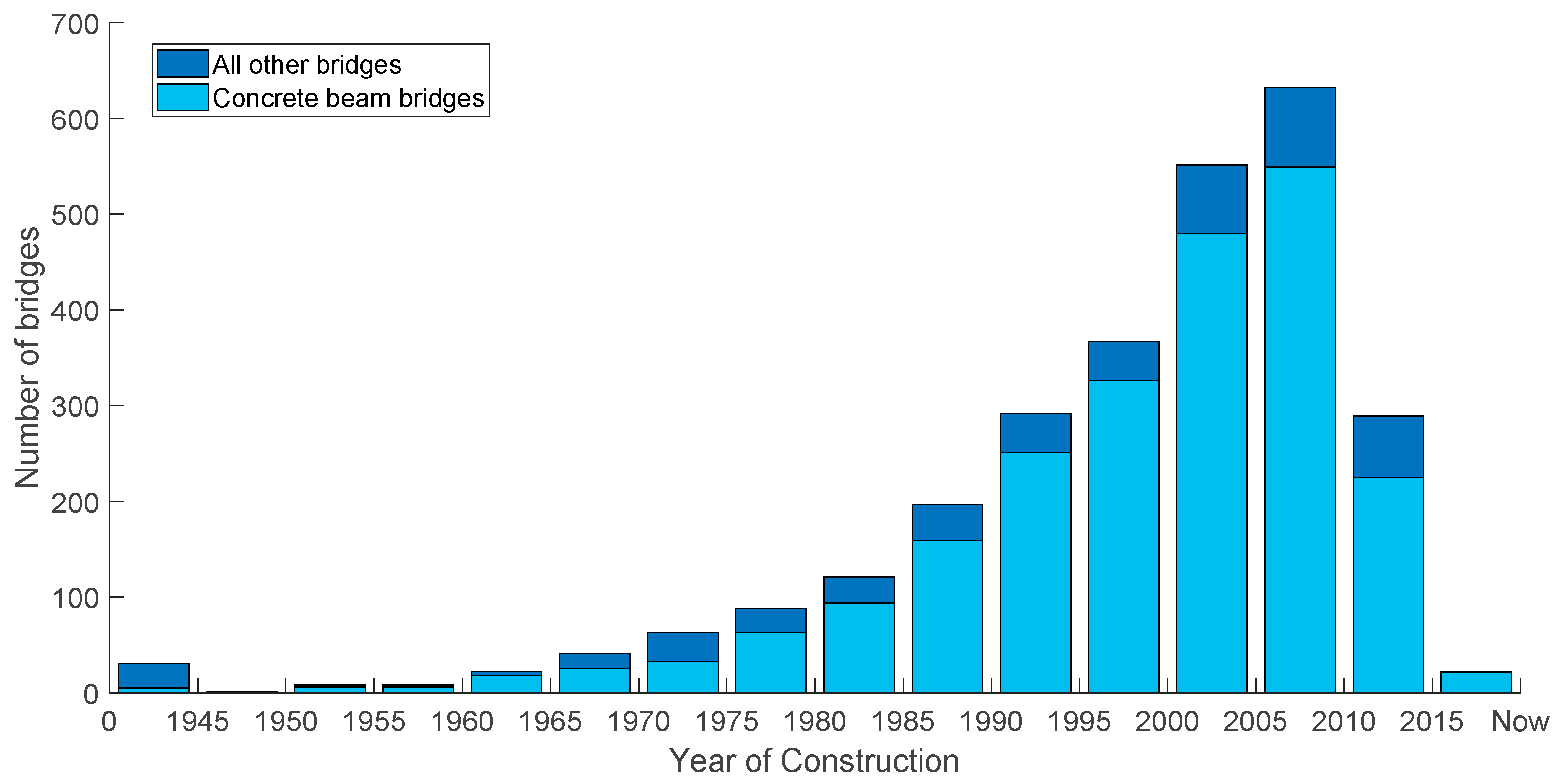
With environmental actions and traffic loads, the performance of urban bridges, especially reinforced concrete (RC) bridges, will deteriorate gradually throughout the bridge service life (i.e., concrete damage and reinforcement corrosion may occur, with cross-section reduction leading to a decrease in the geometric dimensions and materials properties, and thereby to a serviceability degradation or structure failure) [1,2]. Bridge management systems (BMS) have been developing since the early 1990s to assist the management of bridges, which can maximize the network-level bridge performance and minimize the failure probability [3]. Based on the current state evaluation and future bridge condition prediction for the bridge performance, the principal objective of BMS is to develop an effective bridge maintenance, repair, and rehabilitation (MRR) strategy under a limited financial budget [4]. In Shanghai city, the BMS has been applied to the management of small or moderately sized urban bridges since 2004. Therefore, there were 2377 urban bridges across the city included in the BMS database by the end of 2016, in which reinforced concrete beam bridges and prestressed concrete beam bridges account for nearly 85% of the total urban bridge numbers. The construction time of bridges in Shanghai is shown as the following. (Figure 1).

The current state assessment of urban bridges is the foundation of further bridge decay process forecasting and maintenance decision making. In China, the routine evaluation of urban bridges mainly depends on the annual visual inspection, and the bridge condition index (BCI) is used to assess the current state of categories II–V bridges (i.e., small or moderately sized bridges) [5]. Through a hierarchy-weight evaluation method based on bridge components, the whole bridge is comprised of the form “bridge-part-component.” Therefore, the BCI score can reflect the overall technical condition of the whole bridge by comprehensively weighted damage degrees and positions of three major bridge parts (i.e., the deck system, the superstructure, and the substructure) which are made up of other more detailed components [6]. According to the Chinese Technical Code of Maintenance for City Bridge (CJJ 99-2017) [7], BCI scores from 0 to 100 correspond to the bridge condition ratings (CR) from A to E as shown in

Table 1. Chinese bridge condition ratings (CJJ 99-2017).

Rating	BCI Score	Condition	MRR Strategy
A	[90,100]	Intact	Routine maintenance
B	[80,89]	Good	Routine maintenance
C	[66,79]	Qualified	Minor repair
D	[50,65]	Bad	Routine maintenance
E	[0,49]	Dangerous	Minor repair

[6]. It is generally believed that BCI scores evaluated through the annual inspection will affect the MRR strategy of urban bridges in the next year, as shown in Table 1. Where, merely routine maintenance, minor repair, or special inspection is needed for bridges with CR from A to C. As for bridges with CR D or E, medium repair, major repair, or rehabilitation are required in the next year.

The reliability of bridge serviceability behavior will gradually decrease over time due to material degradation, increasing traffic load, and the external environment. Some of the typical problems of RC bridges, namely, concrete carbonization, surface delamination and spalling, crack propagation, steel rebar corrosion, cross-section reduction, and delayed debonding of the external reinforcement may occur [8,9]. The prediction results of the bridge decay process can provide a reliable basis for the further choice of maintenance measures and allocation of finance funds. Accordingly, deterioration forecasting models are essential for the management of urban bridges, especially for network-level or long-term bridge maintenance planning and decision-making. Nevertheless, the existing prediction model for bridge deterioration forecasting in the BMS of Shanghai city still uses the deterministic regression method, which has difficulty reflecting the uncertainty and randomness of the bridge deterioration process. Consequently, this paper proposes a Weibull distribution based semi-Markov process model for the deterioration prediction of urban bridges by considering the time-dependent reliability in the process of bridge deterioration. Consequently, the Weibull distribution was used to characterize the service-life behavior of bridge deterioration within each condition rating (CR) and the semi-Markov process was used to evaluate the transition probabilities of bridge deterioration process between adjacent CRs.

2. Summary of Basic Theory

The bridge deterioration process has often been modeled as the decay of performance over time, which means that the remaining service-life and the future performance of bridges can be forecasted by estimating the rate and pattern of bridge decay. According to different model assumptions, bridge deterioration prediction models can be divided into deterministic models and probabilistic models [10]. Deterministic models assume that the bridge decay trend is specific [11], and mostly estimate the bridge deterioration rate through the regression analysis method. For example, the existing deterioration model in the BMS of Shanghai uses a deterministic regression equation, as shown in Equation (1). Deterministic models have the advantages of simple modeling and convenient correcting [12], but it is quite challenging to reflect the uncertainty and randomness of the deterioration process. Besides, the requirement of high-quality historical data is usually hard to be satisfied, and the preprocessing of original data may also cause a risk of subjective judgment [13].

$$BCI=BC{I}_0[1-\exp {(-\frac{\alpha }{y})}^{\beta }],$$

(1)

where $BCI$ is the bridge condition index, $BC{I}_0=100$ is the initial $BCI$, $y$ is the bridge age, $\alpha$ is the bridge life factor, and $\beta$ is the curve shape factor.

In probabilistic models, bridge deterioration is seen as the result of stochastic processes, and bridge performance can be predicted by describing the probability distribution of the bridge condition state in the future. These models can reflect the uncertainty of bridge deterioration caused by external factors such as traffic loads, materials, environment, and maintenance [14]. Based on the concept of probabilistic cumulative damage, these stochastic models can be further subdivided into state-based or time-based models [15]. The state-based models such as Markov chains are modeled through a discrete-time transition probability matrix from one condition state to another, and the distribution of the future condition is not dependent on the past. Bridge management systems in the U.S like Pontis [16] and BRIDGIT [17] have adopted the Markov chain theory to calculate the bridge deterioration rates [18]. The state-based models have advantages in reflecting the uncertainties of the bridge deterioration process and can be easily applied to network-level bridge management.

Meanwhile, the time-based models such as Weibull distribution assume the duration time of a bridge maintains a condition rating as a random variable which can be modeled through the Weibull probability density functions [19]. Probabilistic models have the advantages of versatility and simplicity, which can clearly describe the service-life behaviors of bridge deterioration (i.e., failure rates, reliability, mean durations, and quantile statistics) [20]. The limitations of probabilistic models lie in need of many accurate observational data and empirical model assumptions [18].

2.1. Defects of Markov Chains

The Markov process describes that a system can be in one of several states, and each state can be passed to another state at a fixed probability over each time step. The Markov chain is a particular case of the Markov process, for which time and state parameters are both discrete. For a stochastic process $\{X(t),t\in T\}$, if the conditional probability can be expressed as Equation (2), then $\{X(t),t\in T\}$ is a Markov chain with discrete parameters [5,21,22].

$$P(X_{t+1}=i_{t+1}|X_0=i_0,X_1=i_1,\cdots ,X_t=i_t)=P(X_{t+1}=i_{t+1}|X_t=i_t),$$

(2)

where $i_t$ is the process state at the time $t$, and $P$ is the conditional probability of a future event.

In Markov-chain based deterioration models, the performance of the bridge changes from one condition state (CR) to another according to a set of transition probabilities, as shown in Equation (3).

$$\begin{array}{cc}P=\left[\left(\begin{array}{ccc}{p}_{11}& \cdots & p_{1n}\\ ⋮& \ddots & ⋮\\ p_{n1}& \cdots & p_{nn}\end{array}\right)\right]& \{\begin{array}{c}\begin{array}{cc}{p}_{ij\ge 0}& i,j\in I\end{array}\\ \begin{array}{cc}{\displaystyle \sum _{j\in I}{p}_{ij=0}}& i\in I\end{array}\end{array}\end{array},$$

(3)

where $P$ is the transition probability matrix, $p_{ij}$ is the transition probability from the state $i$ to the state $j$, and $n$ is the number of bridge condition states.

Therefore, the deterioration process $\{C(t),t\in T\}$ of bridges can be recognized as a stochastic process represented by the initial bridge condition vector $C(0)$ and the transition probability matrix (TPM), as shown in Equation (4).

$$C(t)=C(0)\times P^t,$$

(4)

where $C$ is the condition rating vector, $P$ is the transition probability matrix, and $t$ is the time step.

However, the Markov chain based model has two underlying assumptions, namely, memoryless and homogeneous [9]. Memoryless means the future state of the deterioration process depends only on the current state and has nothing to do with the past, and homogeneous requires the probability of transition from one state to another remain constant throughout the time [23]. Therefore, this paper develops a semi-Markov process model for bridge deterioration prediction in Shanghai. In which, the time-dependent reliability theory was used to characterize the service-life behavior of bridge deterioration within each condition rating (CR) and the semi-Markov process was used to evaluate the transition probabilities of the bridge deterioration process between adjacent CRs. Thus, in the semi-Markov process model, the bridge future state is not only based on the current state but also associated with the history state, and the transition probability from one state to another also could change over time [24].

2.2. Time-Dependent Reliability

When the time-dependent reliability theory can be used to describe the bridge deterioration duration time within an individual CR, the underlying assumption is the existence of a probabilities relationship between the observed CR of discrete-state and the unobserved continuous deterioration process [4]. The CR of bridge performance is treated as a response variable subject to service time and other exponential variables. The bridge performance continues to decay with the increase of time [10]. Furthermore, once the unobserved continuous deterioration reaches or exceeds the threshold of boundaries between different CRs, the time $\left[0,t\right]$ will be recorded as the duration $T_i$ of a particular $CR=i$.

As shown in Equation (5), the cumulative distribution function $F_i(t)$ of the duration $T_i$ in $CR=i$ describes the probability that the bridge will transition out of $CR=i$ by the time $t$.

$$F_i(t)=prob(T_i\le t)={\displaystyle \underset{0}{\overset{t}{\int }}{f}_i(x)}dx,$$

(5)

where $T_i$ is the duration of $CR=i$, and $f_i(t)$ is the probability distribution function of $T_i$.

Moreover, the survivor function $S(T_i)$ is the complement of $F_i(t)$ which means the probability that the bridge element would still be in $CR=i$ by the time $t$, and is defined as Equation (6).

$$S_i(t)=prob(T_i>t)=1-F_i(t),$$

(6)

where $T_i$ is the duration of $CR=i$, and $F_i(t)$ is the cumulative distribution function of $T_i$.

Then the transition probability $p_{ij}(t,\mathsf{\Delta })$ out of $CR=i$ into a worse condition state $CR=j$ within the period $\mathsf{\Delta }$ after the time $t$ can be defined as Equation (7)

$$p_{ij}(t,\mathsf{\Delta })=prob(t<T_i<t+\mathsf{\Delta }|T_i>t)=\frac{F_i(t+\mathsf{\Delta })-F_i(t)}{S_i(t)}=1-\frac{S_i(t+\mathsf{\Delta })}{S_i(t)},$$

(7)

where $T_i$ is the duration of $CR=i$, $F_i(t)$ is the cumulative distribution function of $T_i$, and $S_i(t)$ is the survivor function of $T_i$.

As the complement of $p_{ij}(t,\mathsf{\Delta })$, the transition probability $p_{ii}(t,\mathsf{\Delta })$ of remaining in the same state $CR=i$ can also be given as Equation (8).

$$P_{ii}(t,\mathsf{\Delta })=1-P_{ij}(t,\mathsf{\Delta })=\frac{S_i(t+\mathsf{\Delta })}{S_i(t)},$$

(8)

where $S_i(t)$ is the survivor function of $T_i$.

Therefore, the hazard function $h_i(t)$ which describes the instantaneous rates of failure at the time $t$ given that individual survives up till the time $t$ can be calculated as Equation (9).

$$h_i(T)=\underset{\mathsf{\Delta }\to 0}{\lim }\frac{p_{ij}(t,\mathsf{\Delta })}{\mathsf{\Delta }}=\underset{\mathsf{\Delta }\to 0}{\lim }\frac{F_i(t+\mathsf{\Delta })-F_i(t)}{\mathsf{\Delta }{S}_i(t)}=\frac{f_i(t)}{S_i(t)}i,$$

(9)

where $p_{ij}(t,\mathsf{\Delta })$ is the transition probability from condition rating $i$ to $j$ within the period $\mathsf{\Delta }$, $f_i(t)$ is the probability distribution function of $T_i$, $F_i(t)$ is the cumulative distribution function of $T_i$, and $S_i(t)$ is the survivor function of $T_i$.

2.3. Semi-Markov Process

The transition process between different CRs of bridge deterioration can be described as a semi-Markov process $Y_n$ with $m$ feasible states. The associated random variables $(X_n ,T{S}_n)$ are the successive states and times of the $nth$ transition, and the length of a sojourn time interval $(T{S}_n ,T{S}_{n+1})$ is same as the random variable duration $T_i$ of a specific condition state $X_n=i$ described in the time-dependent reliability theory. The distribution of duration $T_i$ depends on both the state $X_n$ being visited and the state $X_{n+1}$ to be visited next [25].

For many states $i,j=1,2,\cdots ,m$ and the time $t\ge 0$, the associated matrix of the transition probabilities $Q_{ij}$, formally called the semi-Markov kernel can be defined as shown in Equation (10).

$$\begin{array}{ll}{Q}_{ij}(t)& =P(X_{n+1}=j,T{S}_{n+1}-T{S}_n\le t|(X_0,T{S}_0),(X_1,T{S}_1),\cdots (X_n,T{S}_n))\\ & =P(X_{n+1}=j,T{S}_{n+1}-T{S}_n\le t|X_n=i)\end{array}$$

(10)

where $X_n$ is the successive state visited of the $nth$ transition, and $T{S}_n$ is the successive time of the $nth$ transition.

Then the cumulative distribution function $F_i(T)$ is the same as described in Equation (5) which represents the duration $T_i$ in the state $i$ here, can be given as Equation (11).

$$F_i(T)=\mathrm{P}(T{S}_{n-1}-T{S}_n\le t|X_n=i)={\displaystyle \sum _{j=1}^m{Q}_{ij}(t)},$$

(11)

where $Q_{ij}(t)$ is the semi-Markov kernel, and $X_n$ is the successive state visited of the $nth$ transition.

As well known, the eventual transition probability $p_{ij}^e$ shown as Equation (12) represents the probability that the process can move from the state $i$ to the state $j$ neglecting the duration $T_i$ in the state $i$.

$$p_{ij}^e=\underset{t\to \infty }{\lim }{Q}_{ij}(t)=P(X_{n+1}=j|X_n=i),i,j\in E,$$

(12)

where $Q_{ij}(t)$ is the semi-Markov kernel, and $X_n$ is the successive state visited of the $nth$ transition.

Additionally, the matrix $P=[p_{ij}^e]$ is called the transition probability of the embedded Markov chain, and the following conditions must be satisfied:

$$\{\begin{array}{c}{p}_{ij}^e\ge 0\\ {\displaystyle \sum _{i,j=1}^m{p}_{ij}^e\ge 0}\end{array}.$$

(13)

Then the conditional distribution function $G_{ij}(t)$ given both the current state $i$ and next state $j$ can be defined as shown in Equation (14).

$$G_{ij}(t)=P(T{S}_{n+1}-T{S}_n\le t|X_n=i,X_{n+1}=j)=\{\begin{array}{cc}\frac{Q_{ij}(t)}{p_{ij}^e}& p_{ij}^e\ne 0\\ 1& p_{ij}^e=0\end{array},$$

(14)

where $Q_{ij}(t)$ is the semi-Markov kernel, $X_n$ is the successive state visited of the $nth$ transition, and $T{S}_n$ is the successive time of the $nth$ transition.

Therefore, the semi-Markov process kernel $Q_{ij}$ could be defined as:

$$Q_{ij}(t)=p_{ij}^e{G}_{ij}(t),if{p}_{ij}\ne 0,$$

(15)

where $p_{ij}^e$ is the eventual transition probability, and $G_{ij}(t)$ is the conditional distribution function.

Therefore, the transition probability of the semi-Markov process can be defined in the following:

$$p_{ij}(t)=P(X_{n+1}=j|X_n=i),$$

(16)

where is the successive states visited of the $nth$ transitions.

If we assume a semi-Markov process has spent initial time $t_0$ in the state $i$ before the time $t=0$ (i.e., the age of bridge when the observation starts), with a destination state $j$, and the system could go through an intermediate state $l$. Let $\tau$ be the time measured for the stay in the state $i$ from the time $t=0$ to the time of transition to the state $k$. Then the transition probabilities ${\varphi }_{ij}(t)$ of the semi-Markov process can be calculated as following [26]:

$$\begin{array}{ll}{p}_{ij}(t)& ={\delta }_{ij}(1-F_i(t))+{\displaystyle \sum _{l=1}^m{\displaystyle {\int }_0^t{p}_{lj}(t-\tau )}}d{Q}_{il}(\tau )\\ & ={\delta }_{ij}(1-F_i(t))+{\displaystyle \sum _{l=1}^m{\displaystyle {\int }_0^t{Q^{\prime }}_{il}(\tau )p_{lj}(t-\tau )}}d\tau \end{array}$$

(17)

where ${\delta }_{ij}$ is the Kronecker $\delta$ (i.e., if $i=j$, ${\delta }_{ij}=1$ or if $i\ne j$, ${\delta }_{ij}=0$), $F_i(t)$ is the cumulative distribution function, and $Q_{il}(\tau )$ is the semi-Markov process kernel.

Equation (17) is a complicated recursive equation, which can only be solved by Laplace transforms. However, let $h$ be the step measure (i.e., $t=kh$), and using a simplified discretization algorithm. The approximate numerical solution of the transition probability can be calculated as following [27].

$$p_{ij}(kh)={\delta }_{ij}(1-F_i(kh))+{\displaystyle \sum _{l=1}^m({\displaystyle \sum _{\tau =0}^k{w}_{k\tau }{p}_{ij}(kh-\tau h){Q^{\prime }}_{il}(\tau h)}}),$$

(18)

where $h$ is the step measure, ${\delta }_{ij}$ is the Kronecker delta (i.e., if $i=j$, ${\delta }_{ij}=1$ or if $i\ne j$, ${\delta }_{ij}=0$), $F_i(kh)$ is the cumulative distribution function, $w_{k\tau }$ is the weight related to the quadrature formula, and $Q_{il}$ is the semi-Markov process kernel.

3. Deterioration Prediction Model

The BMS has been applied to the management of urban bridges in Shanghai since 2004, and most urban bridges across the city are inspected annually. The original data used in this study is derived from a total of 3185 urban bridge records and 13 years of historical inspection records stored in the BMS database. Besides, the number of inspection data records in the BMS database is as following (

Table 2. Data records in the Bridge Manage System (BMS) database of Shanghai (2004–2016).

Year	All Bridges		Concrete Beam Bridges		Valid Data Records
	Bridge Numbers	Inspection Records	Bridge Numbers	Inspection Records
2004	1390	1091	1116	899	906
2005	1550	1357	1270	1152	830
2006	1601	1447	1335	1248	932
2007	1644	1486	1379	1283	1030
2008	1748	1608	1478	1391	1142
2009	1804	1590	1528	1373	1159
2010	1899	1686	1606	1463	1241
2011	1972	1727	1663	1495	1273
2012	1911	1756	1609	1500	1267
2013	1982	1801	1655	1547	1234
2014	2177	1992	1787	1668	1345
2015	2305	2027	1804	1673	1245
2016	2377	1799	1860	1545	1150
Total	3185	21,367	2468	18,237	14,754

). It should be noted that not every bridge in the database was examined annually, owing to some reasons that include the water level is too high; the bridge is under repair; or the structure form does not apply to the BCI evaluation method.

Although there are a variety of different structural forms of the urban bridges, the concrete beam bridge accounted for most of the total number. The necessary information about these concrete beam bridges is also more accurate than others. Thus, the deterioration process of concrete beam bridges is focused on in this paper.

3.1. Data Preparation Process

It is essential to avoid the interference of the inspector’s subjective deviation and the external intervention of MRR activities, which could guarantee that data is analyzed consistent with the deterioration phenomenon. Therefore, an active process of data preparation is crucial when developing a bridge deterioration prediction model. In this paper, the following main steps of data preparation were used before the development of the deterioration prediction model:

• Cleaning abnormal or null records among the inspection records and bridge ages;
• Filtering inspection records with CR non-monotonically decline or decline over two ratings in two adjacent years;
• Filling the missing records with the same CR value if the CR is the same for three adjacent consecutive years.
• Resetting the age of bridges with rating A which just upgraded from rating D–E to 0;
• Using the analysis-calibration method to set a reasonable data range threshold for bridge ages and CRs based on the bridge engineering experience. (For example, the design service life of urban bridges in China is generally 100 years. Bridges cannot decay from A to D within 20 years, thus determining the lower boundary. Furthermore, bridges cannot remain at A for more than 40 years, then the upper limit of the reasonable data range can be set.)

After the data processing process discussed above, the obtained number of valid data is as shown in the last column of Table 2. For example, in the year of 2016, there are 1150 accurate inspection records of concrete beam bridges meeting the requirement for subsequent analysis and modeling. Overall, the total number of valid data accumulated from 2004 to 2016 is 14,754. Additionally, each of the records contains five sub-records, including the bridge age and CRs of the whole bridge and three main components. For ease of calculation, the condition ratings stored in the BMS database are simplified from a qualitative rating [A, B, C, D, E] to an ordinal system [1, 2, 3, 4, 5].

3.2. Weibull-Distribution Parameter Estimation

Estimation of the reliability function by fitting the distribution parameters of service-life data is the main subject of survival analysis which has been widely used for machine reliability testing and life expectancy prediction. However, when using this method, the presence of censored observation should be taken into account [2,23]. Censored observations are incomplete, and the different influence of the complete, the right-censored, and the left-censored observation is considered as the following [21].

• Complete observation: if a bridge reaches a well-defined threshold value at a certain age, then we have a complete observation about the service lifetime of the bridge.
• Right-censored observation: if a bridge had not reached the threshold value at the time of bridge inspection, then we have a right-censored observation. The right-censored observation can tell us the service lifetime of the bridge goes beyond its present age.
• Left-censored observation: if a bridge had already surpassed the threshold value at the time of inspection, then we have a right-censored observation. The left-censored observation can tell us that the lifetime of the bridges is less than or equal to the present age.

In this paper, the data size of different kinds of observations is shown as in

Table 3. Data size of different observations.

CR	Component Type	Number of Different Observations
		Complete	Right-Censored	Left-Censored
1	Whole bridge	1041	1023	51
	Deck system	1049	912	45
	Superstructure	1016	1112	53
	Substructure	783	1362	54
2	Whole bridge	631	463	36
	Deck system	945	385	35
	Superstructure	555	308	27
	Substructure	691	240	28
3	Whole bridge	234	141	18
	Deck system	832	243	54
	Superstructure	427	158	14
	Substructure	228	28	11
4	Whole bridge	149	16	42
	Deck system	549	68	32
	Superstructure	174	47	15
	Substructure	45	6	8

. Compared with the left-censored observation, the sample number of right-censored observation is relatively large and can be more easily used to estimate parameters. Therefore, the records of left-censored observations were eliminated, and the right-censored observation records were used in the estimation of the Weibull-distribution parameters together with the complete observation records after the tag processing.

The Weibull distribution has been used in the analysis of time-dependent reliability and service life behavior due to its flexibility in fitting different types of service life data. More than that, with different values of the shape parameter $\beta$, the Weibull distribution can be related to a number of other probability distributions such as the normal distribution, the exponential distribution, and even the Rayleigh distribution. Once the Weibull parameters are obtained, the reliability function of Weibull distribution can be used to model a variety of bridge service-life behaviors within different CRs (including the survival function, the hazard function, the mean value, and the quantile statistics).

In this paper, the Weibull distribution method was used to model the observed duration $T_i$, which represents the time of the bridge staying at a particular $CR=i$. The Weibull distribution is mathematically defined by its pdf equation, and the two-parameter pdf expression of Weibull distribution is defined as follows.

$$f(T_i)=\frac{{\beta }_i}{{\eta }_i}{\left(\frac{T_i}{{\eta }_i}\right)}^{{\beta }_i-1}{e}^{-{\left(\frac{T_i}{{\eta }_i}\right)}^{{\beta }_i}},$$

(19)

where $T_i\ge 0$ is the duration, ${\beta }_i>0$ is the shape parameter, and ${\eta }_i>0$ is the scale parameter.

The shape parameter ${\beta }_i$ and scale parameter ${\eta }_i$ of Weibull distribution can be both obtained by fitting the observed durations of the whole bridge, the deck system, the superstructure, and the substructure at different CRs. The estimated results of the Weibull distribution parameters are as shown in

Table 4. Estimated parameters of the Weibull-distribution at different condition ratings (CRs).

CR	Component Type	Estimated Weibull Distribution Parameters
		Shape ${\mathit{\beta }}_{\mathit{i}}$	Scale ${\mathit{\eta }}_{\mathit{i}}$	Mean Value	Standard Deviation
1	Whole bridge	1.458	27.531	24.944	17.388
	Deck system	1.411	25.587	23.293	16.739
	Superstructure	1.421	29.027	26.395	18.838
	Substructure	1.429	37.049	33.663	23.907
2	Whole bridge	1.599	26.025	23.334	14.940
	Deck system	1.510	21.387	19.292	13.022
	Superstructure	1.633	23.881	21.373	13.423
	Substructure	1.484	21.868	19.768	13.555
3	Whole bridge	1.328	31.788	29.237	22.231
	Deck system	1.502	22.127	19.971	13.540
	Superstructure	1.402	22.571	20.567	14.865
	Substructure	1.616	20.832	18.661	11.833
4	Whole bridge	1.217	21.266	19.933	16.461
	Deck system	1.417	19.824	18.034	12.906
	Superstructure	1.315	29.686	27.356	20.996
	Substructure	1.597	23.985	21.508	13.784

.

Through the fitting results of Weibull parameters listed in the above table, we can find that all the shape parameters are never estimated as 1. In which, the Weibull distribution would be the same with exponential distribution as a special case. Therefore, the memoryless and homogeneous assumptions of the Markov chain theory seem invalid in the deterioration process of urban bridges. In fact, the Weibull distributions under the circumstance where ${\beta }_i>1$ are known as wear-out failures, which means the failure rates of concrete beam bridges in Shanghai are increasing with time.

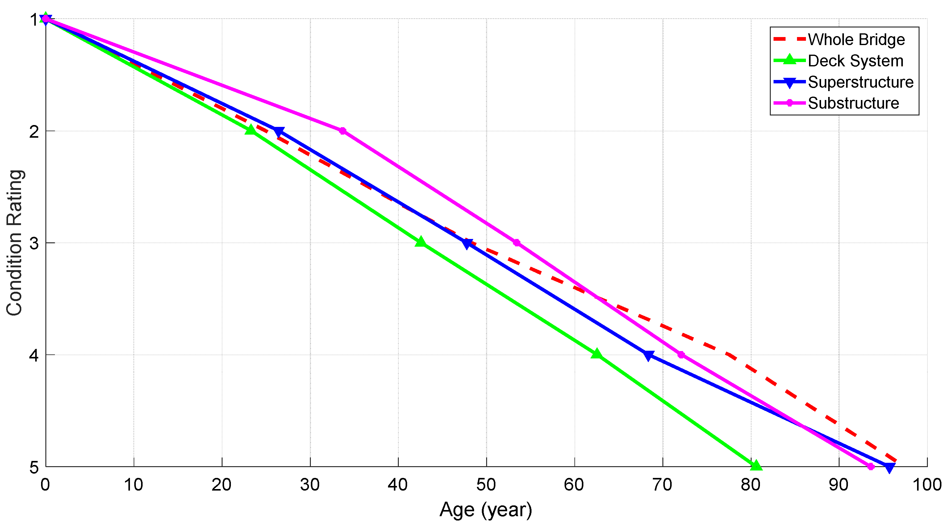
By using the mean value of durations at each CR, the service life expectancy of urban bridges can be predicted, as shown in Figure 2. The prediction result reveals the service life expectancy of concrete beam bridges in Shanghai is about 77 years, while the mean life of the deck system is only 62 years. The decay rate of the deck system is the fastest when compared with the other two parts. Meanwhile, the substructure has a much longer life expectancy, and that is also consistent with the actual bridge maintenance experience. As the bridge deck system directly bears the load effect, which makes components like the deck pavement, expansion joints, etc., more susceptible to damage. The substructure is generally less damaged, and the abutment foundation is relatively stable.

3.3. Semi-Markov Transition Probability Evaluation

As mentioned above, urban bridges in Shanghai are inspected once a year, so the step measure $h$ in Equation (18) could be set to 1. In addition, considering the simplest quadrature method (i.e., rectangle formula) [26], the transition probability $p_{ij}(t)$ can be obtained by the following equation after the necessary simplification [24].

$$\{\begin{array}{ll}{p}_{ij}(t)=S_i(t),& i=j\\ p_{ij}(t)={\displaystyle \sum _k{\displaystyle \sum _{x=1}^t{f}_{ik}(x)}}{p}_{kj}(t-x),& i\ne j\end{array},$$

(20)

where $S_i(t)$ is the cumulative distribution function, $k$ is the intermediate state between $i$ and $j$, and $f_{ik}(x)$ is the probability density function of duration $T_i$ from $CR=i$ to $CR=k$.

In this paper, it was assumed that bridges can degrade no more than two CRs in the interval of two adjacent years, and $t=0$ and $\mathsf{\Delta }=t-x$ were set in Equation (7) [24]. Then the calculation equation of the semi-Markov transition probability can be rewritten as Equation (21).

$$\begin{array}{ll}{p}_{ij}(t)& ={\displaystyle \sum _k{\displaystyle \sum _{x=1}^t{f}_{ik}(x)}}\left[\frac{F_{kj}(t-x)-F_{kj}(0)}{1-F_{kj}(0)}\right],i\ne j\\ & ={\displaystyle \sum _k{\displaystyle \sum _{x=1}^t{f}_{ik}(x)}}{F}_{kj}(t-x)\end{array}$$

(21)

where $f_{ik}(x)$ is the probability density function of duration $T_i$ from $CR=i$ to $CR=k$, and $F_{kj}(t-x)$ is the cumulative density function of duration $T_k$ from $CR=k$ to $CR=j$.

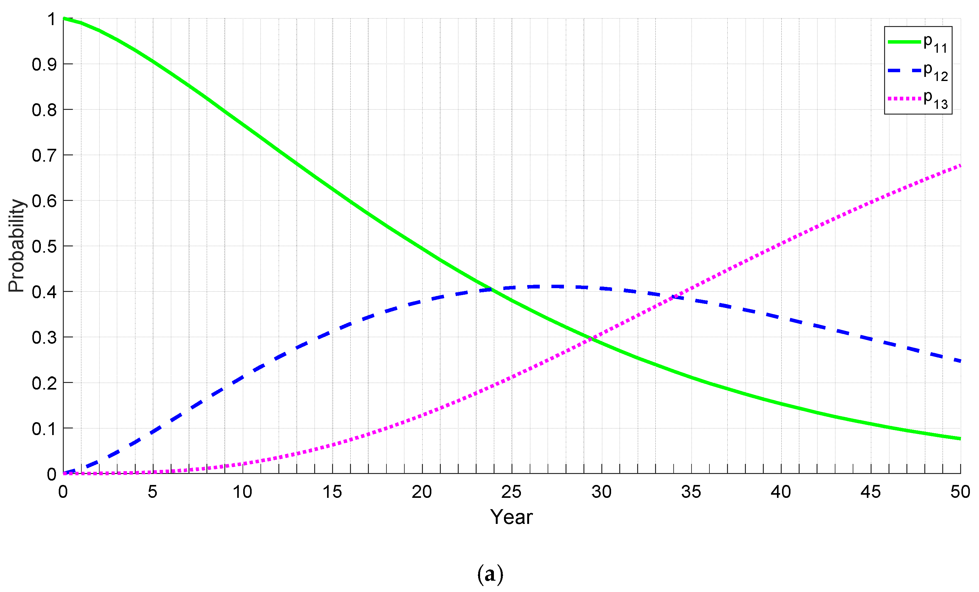
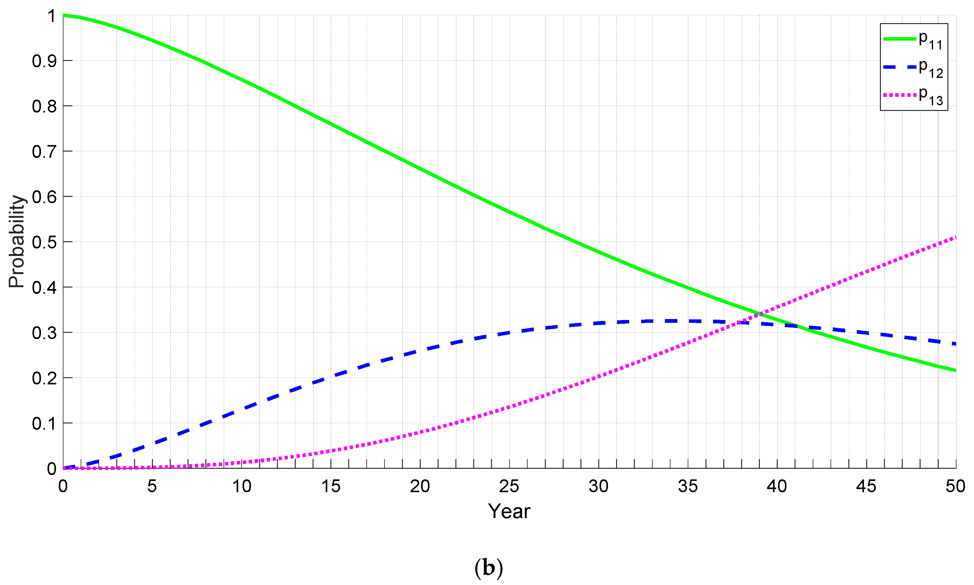
For example, the CR transition probabilities $p_{ij}$ in different years of the deck system and the substructure starting at $CR=1$ can be calculated through the semi-Markov method. As can be seen from Figure 3, transition probabilities of the deck system decay to a worse CR are much larger than the substructure at the same bridge age. The deck system has more than 50% probability that it may decay to $CR=2$ and $CR=3$ after the 19th year, while the substructure has more than half the chance to remain at $CR=1$ till the 28th year. Additionally, the prediction result shows that the deck system has a better chance of remaining at $CR=1$ in the first 24 years and then the deck system will have about 40% probability decay to $CR=2$ between 24 and 34 years. Finally, the deck system will have more than 40% probability transit to $CR=3$ after 34 years later. As for the substructure, transition probabilities of remaining at $CR=1$ are more likely than decaying to $CR=2$ or $CR=3$ in the first 39 years. Then the substructure is more likely to decay to $CR=3$.

4. Discussion

The initial condition $CR(0)$ at the time $t=0$ is needed in the form of a state vector, as shown in Equation (22).

$$CR(0)=\left[\begin{array}{ccccc}{p}_1& p_2& p_3& p_4& p_5\end{array}\right],$$

(22)

where $p_i$ is the proportion of the whole bridge inventory in $CR=i$ at the time $t=0$.

Then the predicted $CR(t)$ of the semi-Markov process would be a product of the initial condition vector and the transition probability matrix, as shown below.

$$CR(t)=CR(0)\times P_{ij}(t),$$

(23)

where $P_{ij}(t)=\left[\begin{array}{ccccc}{p}_{11}(t)& p_{12}(t)& p_{13}(t)& 0& 0\\ 0& p_{22}(t)& p_{23}(t)& p_{24}(t)& 0\\ 0& 0& p_{33}(t)& p_{34}(t)& p_{35}(t)\\ 0& 0& 0& p_{44}(t)& p_{45}(t)\\ 0& 0& 0& 0& 1\end{array}\right]$ is the transition probability matrix of the semi-Markov process at the time $t$.

If we assume the proportion of the whole bridge, the deck system, the superstructure, and the substructure with different CRs in 2016 as the initial proportion of the bridge inventory, then the future CR proportion change caused by performance deterioration can be predicted through the semi-Markov process model. The comparison between prediction results of the semi-Markov method and the regression analysis method currently used by Shanghai BMS in 2017 and 2018 are shown in

Table 5. Comparison of the regression analysis and semi-Markov model prediction results.

CR	Prediction Model	2017			2018
		Actual Value	Expected Value	Relative Error	Actual Value	Expected Value	Relative Error
1	Regression analysis	52.40%	46.34%	11.56%	52.24%	38.47%	26.36%
	Semi-Markov		49.36%	5.81%		48.67%	6.83%
2	Regression analysis	39.61%	13.73%	65.34%	41.27%	20.84%	49.51%
	Semi-Markov		41.72%	5.32%		41.94%	1.63%
3	Regression analysis	7.15%	28.22%	294.73%	5.82%	28.99%	398.25%
	Semi-Markov		7.59%	6.18%		7.93%	36.32%
4	Regression analysis	0.80%	9.62%	1103.57%	0.59%	9.62%	1541.58%
	Semi-Markov		1.22%	52.25%		1.29%	119.29%
5	Regression analysis	0.04%	2.09%	4606.68%	0.08%	2.09%	2396.51%
	Semi-Markov		0.12%	165.75%		0.16%	95.55%

. The predicted values of the semi-Markov method are closer to the actual values, while the traditional approach has a significant deviation. It suggests that the overall prediction accuracy of the semi-Markov model is better than the regression analysis method. The relative errors of the semi-Markov model for bridges at $CR=1$ are nearly 6% while the traditional ones are more than 10%. Furthermore, for bridges at $CR=2$, the relative errors are less than 6% of the proposed model; however, the traditional model has about 50% relative error. As for bridges at $CR=3$, when the relative errors of the conventional method are about 300%, the relative error of the new approach is 5% in 2017 and 35% in 2018. For bridges with more deteriorated CRs, smaller data size and external interference may have negative impacts on deterioration prediction. However, compared to the large deviations of the regression analysis, the prediction accuracy of the semi-Markov model for bridges at $CR=4$ and $CR=5$ is also acceptable.

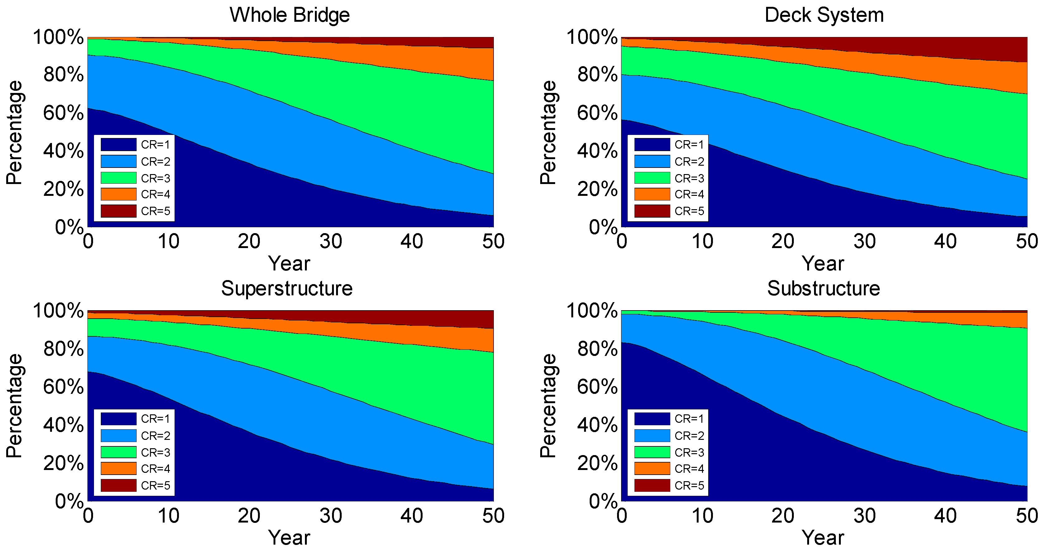
As shown in Figure 4, the Weibull distribution based semi-Markov process bridge deterioration model can be used to predict the overall deterioration trend of urban bridges at network-level. It is easy to find that the overall decay rate of the deck system is the fastest, the superstructure is the second, and the substructure is the slowest. As for the whole bridge, there will be about 51% of bridges remaining in $CR=1$, 34% remaining in $CR=2$, and 12% remaining in $CR=3$ in the next decade. It follows that the proportion of bridges with $CR=1$ will gradually decrease, while the proportion of bridges with $CR=3$ and $CR=4$ will increase rapidly within the next 50 years. The predicted results are in a good agreement with the actual degrade trend of the overall urban bridges in Shanghai. In order to reduce the bridge maintenance pressure in the future, it is necessary to adopt a targeted preventive maintenance strategy and to delay the decay rate of bridge performance.

5. Conclusions

The performance of urban bridges will gradually deteriorate with the increase of service time. The existing bridge deterioration prediction model of the BMS in Shanghai uses the regression analysis method. This paper proposed a Weibull distribution based semi-Markov process prediction model by using the bridge inspection data in BMS since 2004. The Weibull distribution was used to characterize the bridge service-life behavior of duration time within each CR, and the semi-Markov process was used to evaluate the transition probabilities of bridge deterioration between different CRs. The service life expectancy of urban bridges, the transition probabilities of the deck system and the substructure, and the future CR proportion change caused by deterioration was predicted.

The prediction result reveals that the estimated shape parameters of Weibull distribution are all larger than 1, which indicates the failure rates of urban bridges in Shanghai are not homogeneous but increase with time. The service life expectancy of concrete beam bridges in Shanghai is about 77 years. Among the three major parts of urban bridges, the decay rate of the deck system is the fastest, and the substructure has a much longer life expectancy. It may be because the bridge deck system directly bears the load effect, which makes it more susceptible to damage. By comparison, the overall prediction accuracy of the semi-Markov model is better than the regression analysis method. It follows that the proportion of bridges $CR=1$ with $CR=2$ will gradually decrease, while the proportion of bridges with $CR=3$ and $CR=4$ will increase rapidly within the next 50 years. The prediction results show it is necessary to strengthen the maintenance of the deck system and adopt a preventive maintenance strategy for bridges now with less deteriorated CRs to reduce the future bridge maintenance pressure.

Compared with the existing regression analysis method, the Weibull distribution based semi-Markov process bridge deterioration model can describe the performance decay behavior of the bridge in more detail, and the prediction accuracy is relatively higher. Therefore, when the data size of historical bridge inspection records is big enough, this model can be well applied to the deterioration prediction of urban bridges both at project-level and network-level. At the same time, the proposed model can provide some basis for bridge maintenance decision-making and financial allocation optimization.

References

- Foraboschi, P. Analytical model to predict the lifetime of concrete members externally reinforced with FRP. Theor. Appl. Fract. Mech. 2015, 75, 137–145. [Google Scholar] [CrossRef]
- Branco, F.A.; Brito, J.D. Handbook of Concrete Bridge Management; American Society of Civil Engineers: Reston, VA, USA, 2004. [Google Scholar]
- Morcous, G. Performance prediction of bridge deck systems using Markov chains. J. Perform. Constr. Fac. 2006, 20, 146–155. [Google Scholar] [CrossRef]
- Mishalani, R.G.; Madanat, S.M. Computation of infrastructure transition probabilities using stochastic duration models. J. Infrastruct. Syst. 2002, 8, 139–148. [Google Scholar] [CrossRef]
- Li, L.; Li, F.; Chen, Z.; Sun, L. Use of Markov Chain Model Based on Actual Repair Status to Predict Bridge Deterioration in Shanghai, China. Transp. Res. Record 2016, 2550, 106–114. [Google Scholar] [CrossRef]
- Fang, Y.; Li, L.; Chen, Z.; Sun, L. Prediction Model of Concrete Girder Bridge Deterioration in Shanghai Using Weibull-Distribution Method. 2017. Available online: https://trid.trb.org/view/1438643 (accessed on 8 December 2016).
- China, M.O.C.O. Technical Code of Maintenance for City Bridges. S. In CJJ 99-2003, China; 2017. Available online: http://www.mohurd.gov.cn/wjfb/201801/t20180104_234665.html (accessed on 31 July 2017).
- Foraboschi, P. Shear strength computation of reinforced concrete beams strengthened with composite materials. Compos.: Mech. Comput. Appl.: Int. J. 2012, 3, 227–252. [Google Scholar] [CrossRef]
- Foraboschi, P. Structural layout that takes full advantage of the capabilities and opportunities afforded by two-way RC floors, coupled with the selection of the best technique, to avoid serviceability failures. Eng. Fail. Anal. 2016, 70, 387–418. [Google Scholar] [CrossRef]
- Agrawal, A.K.; Kawaguchi, A.; Chen, Z. Deterioration rates of typical bridge elements in New York. J. Bridge. Eng. 2010, 15, 419–429. [Google Scholar] [CrossRef]
- Lu, P.; Pei, S.; Tolliver, D.; Jin, Z. Data-based Evaluation of Regression Models for Bridge Component Deterioration. 2015. Available online: https://trid.trb.org/view/1337198 (accessed on 30 December 2014).
- Chen, Z. Research on Technology Structure of Transportation Infrastructure Management System. Ph.D. Thesis, Tongji University, Shanghai, China, July 2005. [Google Scholar]
- Zambon, I.; Vidovic, A.; Strauss, A.; Matos, J.; Amado, J. Comparison of stochastic prediction models based on visual inspections of bridge decks. J. Civ. Eng. Manag. 2017, 23, 553–561. [Google Scholar] [CrossRef]
- Su, D.; Nassif, H.; Hwang, E. Probabilistic Approach for Forecasting Long Term Performance of Girder Bridges. 2015. Available online: https://trid.trb.org/view/1339284 (accessed on 30 December 2014).
- Madanat, S.; Mishalani, R.; Ibrahim, W.H.W. Estimation of infrastructure transition probabilities from condition rating data. J. Infrastruct. Syst. 1995, 1, 120–125. [Google Scholar] [CrossRef]
- Golabi, K.; Shepard, R. Pontis: A system for maintenance optimization and improvement of US bridge networks. Interfaces 1997, 27, 71–88. [Google Scholar] [CrossRef]
- Hawk, H.; Small, E.P. The BRIDGIT bridge management system. Struct. Eng. Int. 1998, 8, 309–314. [Google Scholar] [CrossRef]
- Reardon, M.F.; Chase, S.B. Migration of Element-Level Inspection Data for Bridge Management System. 2016. Available online: https://trid.trb.org/view/1392750 (accessed on 1 December 2016).
- Ng, S.K.; Moses, F. Prediction of bridge service life using time-dependent reliability analysis. Bridge Manag. 1996, 3, 26–32. [Google Scholar]
- Medjoudj, R.; Aissani, D.; Boubakeur, A.; Haim, K.D. Interruption modelling in electrical power distribution systems using the Weibull—Markov model. Proc. Inst. Mech. Eng. Part O: J. Risk Reliab. 2009, 223, 145–157. [Google Scholar] [CrossRef]
- Madanat, S.M.; Karlaftis, M.G.; McCarthy, P.S. Probabilistic infrastructure deterioration models with panel data. J. Infrastruct. Syst. 1997, 3, 4–9. [Google Scholar] [CrossRef]
- Micevski, T.; Kuczera, G.; Coombes, P. Markov model for storm water pipe deterioration. J. Infrastruct. Syst. 2002, 8, 49–56. [Google Scholar] [CrossRef]
- Wellalage, N.W.; Zhang, T.; Dwight, R.; El-Akruti, K. Bridge deterioration modeling by Markov Chain Monte Carlo (MCMC) simulation method. In Engineering Asset Management-Systems, Professional Practices and Certification; Springer: Cham, Switzerland, 2015; pp. 545–556. [Google Scholar]
- Sobanjo, J.O. State transition probabilities in bridge deterioration based on Weibull sojourn times. Struct. Infrastruct. E 2011, 7, 747–764. [Google Scholar] [CrossRef]
- Ng, S.; Moses, F. Bridge deterioration modeling using semi-Markov theory. A. A. Balkema Uitgevers B. V, Struct. Saf. Reliab. 1998, 1, 113–120. [Google Scholar]
- Corradi, G.; Janssen, J.; Manca, R. Numerical treatment of homogeneous semi-Markov processes in transient case—A straightforward approach. Methodol. Comput. Appl. 2004, 6, 233–246. [Google Scholar] [CrossRef]
- Kallen, M.J.; Van Noortwijk, J.M. Statistical Inference for Markov Deterioration Models of Bridge Conditions in the Netherlands. 2006. Available online: http://citeseerx.ist.psu.edu/viewdoc/download?doi=10.1.1.74.5105&rep=rep1&type=pdf (accessed on 2 March 2015).
Figure 1.
The distribution of bridge construction by year in Shanghai.
Figure 2.
Deterioration prediction of urban bridges at different CRs.
Figure 3.
Semi-Markov transition probabilities change with bridge service time: (a) transition probability of the deck system; (b) transition probability of the substructure.
Figure 4.
Prediction of the concrete beam bridge deterioration in Shanghai.