Customized Bus Network Design Based on Individual Reservation Demands

1
Beijing Key Laboratory of Traffic Engineering, Beijing University of Technology, Beijing 100124, China
2
School of Civil Engineering, Henan University of Technology, Zhengzhou Henan 450001, China
3
Beijing Jinghang Research Institute of Computing and Communication, Beijing 100074, China
4
Research Institute of Highway Ministry of Transport, Beijing 100088, China
*
Author to whom correspondence should be addressed.
Sustainability 2019, 11(19), 5535; https://0-doi-org.brum.beds.ac.uk/10.3390/su11195535
Submission received: 19 September 2019
/
Revised: 4 October 2019
/
Accepted: 6 October 2019
/
Published: 8 October 2019
Abstract
:With the advantages of congestion alleviation, environmental friendliness, as well as a better travel experience, the customized bus (CB) system to reduce individual motorized travel is highly popular in increasing numbers of cities in China. The line planning problem is a key aspect of the CB system. This paper presents a detailed flow chart of a CB network planning methodology, including individual reservation travel demand data processing, CB line origin–destination (OD) area division considering quantity constraints of demand in areas and distance constraints based on agglomerative hierarchical clustering (AHC), an initial set of CB lines generating quantity constraints of the demand on each line and line length constraints, and line selection model building, striking a balance between operator interests, social benefits, and passengers’ interests. Finally, the impacts of the CB vehicle type, the fixed operation cost of online car-hailing (OCH), and the weights of each itemized cost are discussed. Serval operating schemes for the Beijing CB network were created. The results show that the combination of CB vehicles with 49 seats and 18 seats is the most cost-effective and that CBs with low capacity are more cost-effective than those with larger capacity. People receive the best service when decision-makers pay more attention to environmental pollution and congestion issues. The CB network’s service acceptance rate and the spatial coverage increase with the fixed operating cost per OCH vehicle per day . The CB vehicle use decreases as increases. The results of this study can provide technical support for CB operators who design CB networks.
1. Introduction
The public transport service is facing problems with overcrowding, low punctuality, and the amount of time taken to travel in peak periods, which greatly affect the satisfaction of passengers with the public transport service and reduces the attraction of public transport. Thus, more people are forced to choose private cars, taxis, and online car-hailing (OCH). However, the increase in these individual motorized services has presented a number of challenges: the risk of increased vehicular travel and reduced public transit use, increased congestion, and shifts in mobility patterns, which are difficult to predict [1]. These individual motorized travel modes are characterized by low resource use and high travel costs. To sustainably meet these challenges, considering congestion, environmental impacts, and fuel consumption, new forms of transport must be explored [2].
Big traffic data have enabled the creation of innovative traffic services. The combinations of big data, mobile Internet, artificial intelligence, and cloud computing have led to many new forms of Mobility as a Service (MaaS). With the help of pedestrian–vehicle positioning, online reservation, and electronic payment technologies, MaaS can accurately and quickly respond to mass personalized travel demands and provide a variety of options for travelers. On the basis of meeting individual travel needs, individual motorized travel can be guided to customized bus (CB) travel based on big data. These technologies help with realizing the innovation of traffic service modes and the intensive transformation of traffic demand. CBs can provide direct and efficient transit services for groups of commuters with similar travel demands [3], which is conducive to improving dweller trip structure, alleviating traffic congestion, and reducing environmental pollution. A comparison of CB with OCH and conventional buses is provided in Table 1.
Demand-responsive transit (DRT) systems are a class of transit services in which a fleet of vehicles dynamically changes routes and schedules to accommodate demand within a service area and can flexibly provide service [4]. Amirgholy and Gonzales [4] employed an analytical model to approximate the agency’s operating cost for running a DRT system with dynamic demand and the total generalized cost that users experience as a result of the operating decisions. Flexible transit services combine the characteristics of fixed-route public transit and a demand-responsive service and are able to replace the conventional public transit service under many conditions. The demand-responsive connector is one of these flexible transit services and has already been operated as feeder transit in some cities [5]. Shen et al. [5] proposed a two-stage routing model to minimize the system cost, considering both the service provider and riders, to address the vehicle routing operation problem of the demand-responsive connector system with on-demand stations. Chen and Nie [6] analyzed a demand-adaptive service that connects passengers from their origin/destination to the fixed-route service to improve accessibility.
The CB is a new and innovative mode of DRT system that provides an advanced, attractive, and user-oriented service to specific clientele, especially commuters, by aggregating their similar travel-demand patterns using online information platforms, such as the Internet, telephones, and smartphones [7]. In terms of a customized service, route design plays a vital role in the CB operation system [8]. Li et al. [9] established a real-time scheduling model for single-line CB transit to optimize the system. The CB line that was studied was a fixed line with fixed stations and passenger reservation was known. Only one type of bus was considered in this study.
The CB service design problem involves the optimization of a set of vehicle routes, the layout of pick-up and drop-off stations, and timetables. Tong et al. [10] developed a joint optimization model to address several important practical issues: (1) how to formulate a holistic traveler mobility optimization approach to determine bus stops, passenger-to-vehicle assignment, and detailed bus route and schedule; and (2) how to integrate and solve capacitated trip-to-bus assignment and bus timetabling problems for large-scale networks. Ma et al. [11] proposed a methodological framework for CB network design using a questionnaire data collected on the Internet. Conducting online surveys is passive and limited, as well as inefficient and costly in investigating all the OD without a specific aim [12]. Ma et al. [13] studied the problems associated with the operation of CBs, such as stop selection, line planning, and timetables, and established a model for CB stop planning and timetables. Li et al. [14] established a mixed-load CB routing model with a time window which is a mixed integer programming model. Guo et al. [8] developed a mixed integer programming model to formulate a CB multivehicle routing problem, providing suggestions for bus stop locations and routes. The model can determine passenger-to-vehicle assignment based on a series of constraints, such as operation standards and the number of stations. Li et al. [12] proposed a methodological framework of extracting potential CB routes from bus smart card data, which consisted of three processes: trip reconstruction, OD area division, and CB route extraction. Lyu et al. [3] proposed a CB line planning framework called CB-Planner, which is applicable to multiple travel data sources. Issues including bus stop locations, bus routes, timetables, and passengers’ probabilities of choosing CB were simultaneously optimized by a mathematical programming formulation.
In the field of CB stop deployment, Lyu et al. [15] formulated the CB stop deployment problem as a facility location problem, which aims to find the minimum number of stops and their optimal locations, such that these stops can cover at least a given coverage percentage of passengers within the given coverage radius of a stop. They employed integer linear programming to find the best locations for CB stops. Lyu et al. [3] developed a heuristic solution framework that includes a grid-density-based clustering method for efficiently discovering potential travel demands, a CB stop deployment algorithm to minimize the number of stops and walking distance, and dynamic-programming-based routing and timetabling algorithms for maximizing estimated profit.
The determination of recommended taxi pick-ups can be used for reference in the determination of CB stops. Based on spatio-temporal clustering, Zhang et al., [16] proposed a method of recommending pick-ups for taxi drivers using taxi global positioning system (GPS) data. Zhu et al. [17] invented a method to select a recommended pick-up point by integrating various traffic influencing factors to ensure that the setting of the pick-up point is compatible with the actual traffic situation.
As an on-demand transport service, taxis play an important role in urban systems, and the pick-up and drop-off locations in taxi GPS trajectory data have been widely used to detect urban hotspots for various purposes [18]. Lyu et al. [15] proposed a bus line planning framework, called T2CBS, by taking full advantage of taxi trajectory data. Based on taxi GPS trajectory data from Shenzhen, China, Hu et al. [19] explored taxi drivers’ operation behavior and passengers’ demand. Ma et al. [20] modeled and analyzed the changes in the daily driving patterns of taxis in a disrupted market by mining large-scale taxi trajectory data sets, and distinct patterns were extracted using the k-means clustering method. Liu et al. [21] proposed a unified framework to design, optimize and analyze mobility-on-demand operations, and calibrated the proposed framework using the taxi demand data.
Online car-hailing apps/platforms have emerged as novel and popular means to provide an on-demand transportation service via mobile apps [22]. However, few studies have focused on mining the travel demand using OCH travel data. Wang et al. [22] presented a supply–demand prediction framework for online car-hailing services using deep neural networks that can automatically discover complicated supply–demand patterns from the car-hailing service data. Jiang et al. [23] proposed a short-term demand prediction method for an OCH service based on a least squares support vector machine using network car order data as the network car demand data to test the model.
Using latitude and longitude data, the main clustering methods used to determine specific function point are k-means clustering, the density-based spatial clustering of applications with noise (DBSCAN), and hierarchical clustering. The k-means algorithm is used to cluster commuting data, which are presented on longitude and latitude coordinates assuming that each centroid of the clusters would be reasonable locations of vertiports for personal air vehicles [24]. Lyu et al. [15] extended the traditional density-based clustering algorithm DBSCAN to an algorithm T-DBSCAN, to cluster trajectories with nearby pick-up and drop-off points and similar pick-up timestamps. Li et al. [12] use an improved DBSCAN algorithm to address the OD area division and CB route extraction to extract potential CB routes based on bus smart card data. Zhen et al. [25] used the improved hierarchical clustering algorithm based on density clustering to create the same OD clustering, which used the Integrated Circuit (IC) card data and the public transport GPS data to extract passengers’ travel OD data. Luo et al. [26] proposed an algorithm to extract the hotspot areas of urban residents with a hierarchical clustering method using the stop-point data obtained from a mobile phone travel survey. Pusadan et al. [27] used agglomerative hierarchical clustering (AHC) to determine the optimal waypoints of the flight route in several segments based on range area coordinates (latitude and longitude) of every waypoint. Euclidean distance was used to measure distances between waypoints with two centroids as a result of clustering AHC.
In the above studies, the data used in CB line planning were generally taxi trajectory data and an online questionnaire, and few studies used OCH data. The constraints of minimum demand and length limitation were not considered by Ma et al. [11] during the CB line of area division and line OD area pairing. Studies tended to only consider one type of bus. As such, our contributions are as follows: (1) based on hierarchical clustering, the CB network is planned using OCH data; (2) in the four steps of CB network planning, line length and minimum demand constraints are proposed to reduce computational redundancy; and (3) based on the line selection model proposed by Ma et al. [11], the cost factors are improved, and a model considering multiple CB vehicles types is constructed.
This paper is organized as follows. Section 2 presents the process and details of CB network planning, outlining the building of the line selection model. Section 3 describes the case analysis based on the CB network planning method. Sensitivity was analyzed to reveal the influence of CB vehicle types, cost factor weights, and the fixed operating cost in Section 4. Section 5 provides concluding remarks and future research work.
2. CB Network Design Methodology
2.1. CB Network Design Processing
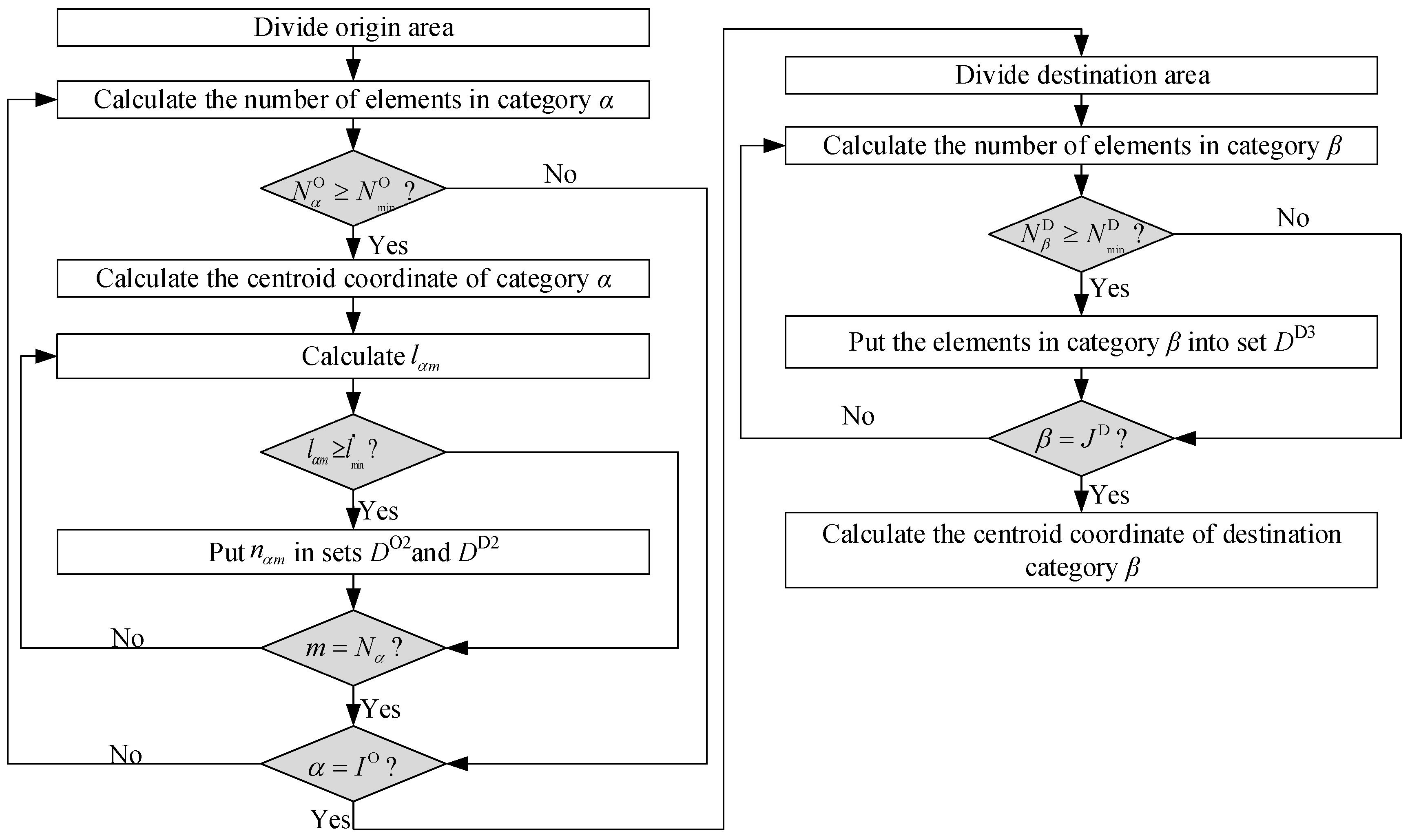
The CB line planning process mainly involves the following four steps, as shown in Figure 1:
(1) Processing the individual travel booking demand data: The individual travel booking demand data processing mainly involves screening and cleaning data, for which the OD linear distance constraint is used. Based on longitude and latitude data, ArcGIS 10.2 (Esri, USA) was used to convert them into plane coordinates to provide data support for network planning.
(2) Dividing CB line OD areas: Passengers board a CB at the origin area stops and alight at the destination stops, which are non-fixed stops. One stop at each point of demand makes the whole operation time too long and increases the operation cost. However, sharing the same station by passengers who are far away causes the CB to lose its door-to-door advantage. Therefore, a stop should serve areas in which the distance between passengers’ origins or destinations is within a reasonable range. Hierarchical-clustering-based origin–destination (OD) region division is used to find CB stop areas to be selected in CB network planning. The service area of a bus stop is determined by the radius of area division. The line length and minimum demands need to be met to reduce the calculation amount and rationally use resources. The element number constraints and distance constraints are taken into consideration in the OD region division in which the line OD areas and demands in each OD area are obtained.
(3) Generating an initial set of CB lines: Based on the results of CB line OD area division, a series of lines is gained by pairing the origin areas with the destination areas. The travel demands with the same order number in both origin areas and destination areas on this line are the demands on the line. Then, the travel demand OD table is created. The lines satisfying the line length and element number constraint settings are preserved, which form the initial set of lines. This can reduce the calculation amount in the next step.
(4) Establishing the CB line selection model: The CB is a kind of green and intensive public transportation. It can effectively reduce personalized motorized travel, thus reducing energy consumption, pollution emissions, and road congestion. Since not all lines in the initial set of CB lines are suitable for running CBs, a model is needed to determine whether each line is suitable for providing CB services. The operating lines and CB network scheme are determined by setting up a generalized cost objective function about the operating cost, social benefits, and the cost of passengers whose input is the standard of CB line operation.
We made the following assumptions in this study: (1) passengers travel by either CBs or OCH; (2) each bus only runs one route and starts from the origin area and ends in the destination area; (3) passengers can only board in the origin areas and alight in the destination areas; and (4) the CB line length is represented by the average travel distance of all the travel demands on this line.
The sets, indices, and parameters used in this study are listed in the Appendix A.
2.2. Individual Reservation Travel Demand Data Processing
The order data of OCH are the record of completing an OCH service. We selected a few fields that are useful for CB network planning, including the order number, the information about when and where the OCH passengers get on and off, passenger mileage, and passengers’ due expenses, which are shown in Table 2.
The specific data processing steps were as shown in Figure 2. We eliminate the data with a linear distance less than . According to Ma et al. [11], the area coverage radius is 2.5 km, and the minimum length of the line operation is determined to be . Hence, the demands with a line distance less than are not within the service range of the CB. Then, ArcGIS (Esri, USA) was used to convert longitude and latitude coordinates into plane coordinates.
2.3. CB Line OD Area Division
Cluster analysis is a main task in exploratory data mining and a common technique for statistical data analysis, which is an important field of unsupervised learning. Cluster analysis involves attempting to divide the samples in a data set into several disjoint subsets, and each subset is called a “cluster” [28]. Hierarchical clustering is suitable for the CB travel demand clustering, which is one of the typical cluster models [11].
Hierarchical clustering, also known as connectivity-based clustering, is based on the core idea of objects being more related to nearby objects than to objects farther away. These algorithms connect objects to form clusters based on their distance. Agglomerative hierarchical clustering (AHC) is a bottom-up approach: each observation starts in its own cluster, and pairs of clusters are merged when moving up the hierarchy [29]. The metric for hierarchical clustering used in this study was Euclidean distance. The maximum distance between elements of each cluster (also called complete-linkage clustering) is used as the linkage criteria between two sets of observations A and B used in this paper. The specific process is as follows, as shown in Figure 3:
Step 1. The origins of demands in Section 2.2 are classified using AHC. The number of elements (observed objects) in each category is obtained.
Step 2. The centroid coordinate of each category is calculated. A centroid is the means of the observations in one cluster, whose method of calculation is given by Ma et al. [11]. If , the category is retained; otherwise, it is deleted. The line distance between the centroid and destination of the arbitrary element m in each origin category and is calculated; that is, we calculate the distances from the destinations of all observed objects to the centroid in each category. If , the element m is retained; otherwise, it is deleted from the category . In this paper, and .
Step 3. Repeat Step 2 until all elements (observed objects) and categories (origin areas) are verified.
Step 4. The destinations of the demands are classified using AHC. The number of elements in each category is determined.
Step 5. If , the category is retained; otherwise, it is deleted.
Step 6. Repeat Step 5 until all elements (observed objects) and categories (destination areas) are verified.
Step 7. Calculate the centroid coordinate of each destination category. is set to avoid situations in which the origin and destination of the same demand is in the same class.
2.4. Initial Set of CB Lines Generating
A line set containing lines is obtained by paring the O and D areas. According to Ma et al. [11], the minimum length of the line operation is determined to be . If the demands on one CB line are too low—for instance, less than (because of this, CB occupancy must be guaranteed to be at least 50%, and the maximum load capacity per CB vehicle is 18 people/bus, meaning that is determined to be 9)—there is no need to operate CB vehicles on the line. To improve the efficiency of the CB network planning process, the lines which do not satisfy the demand constraints do not need to be considered in the following line selection model, as shown in Figure 4.
2.5. Line Selection Model Building
A CB transport system involves stakeholders, including both suppliers and demanders, as well as the overall interests of society. CB operation increases the operating costs of CB suppliers, and the CB passengers should pay bus fares. However, this will reduce vehicle pollution emissions and ease traffic congestion, which are overall benefits to society. The problem with line selection is creating a multi-faceted comprehensive balance. Therefore, the generalized costs of the CB system in this study mainly include the company’s operating cost, environmental cost, traffic congestion cost, and tge passenger cost.
The company’s operating cost is determined using the following function:
where the first part of Equation (1) is the fuel costs of CBs related to mileage, and the second part is the fixed operating costs of CBs related to vehicle purchase expense, taxes and dues, vehicle repair and maintenance costs, the depreciation of vehicles, and the driver’s salary. The third and fourth parts of Equation (1) are the fuel cost and fixed cost of OCH, respectively, which were not considered by Ma et al. [11].
The environmental cost is calculated as
The traffic congestion cost is determined using the following function:
The cost of fares paid by passengers is calculated as follows:
where the first part of Equation (4) is the fare paid by all CB passengers on line i, the second part is the fare paid by all OCH passengers on line i, and represents the interest of passengers, which was not considered by Ma et al. [11].
Based the model built by Ma et al. [11], the objective function of the line operating standard model can be determined using the linear weighted sum of the four parts as
where the weights , , and could be determined based on Ma et al. [11].
The number of passengers taking CB and the number of passengers taking OCH are the decision variables. As can be seen from Formulas 1–5, varies with the fixed operating costs, the type of CB vehicles or weights , , and . In addition, the number of CBs required, the CB line length and the service level are also different.
One constraint is that CB occupancy must be guaranteed to be at least 50%:
According to the existing travel experience, the length of a CB line is set as the average travel distance corresponding to the travel demand of the routes:
To ensure no excessive waste of resources, the length of CB lines and the travel demand on the lines must meet certain requirements; that is, the length of the CB lines must be greater than the minimum length, and the travel demand must be greater than the minimum demand:
The principle of demands is that the number of passengers taking CB vehicles of type j plus the number of passengers taking OCH should be equal to the amount of total travel demand on the line i, which is known.
is the number of OCH vehicles on each line, formulated as
Solving the CB line selection model is an integer programming problem and a discrete optimization problem [11]. The branch-and-bound method was used to solve the model in MATLAB (MathWorks, USA). The number of passengers served by the CB and OCH on each line can be calculated. The lines selected for running CBs are those on which the number of CB passengers is greater than zero; otherwise, the lines are operated by OCH. The number of CB vehicles on each CB line is thus obtained.
2.6. Service Level Evaluation
Based on the research of Ma et al. [11], the following evaluation indexes are established to evaluate the service level of the CB network.
The service rate is the proportion of the total number of people served by CBs to the number of reservation demands, which can be presented as
The average load factor is the proportion of the total number of people served by CBs to the maximum number of seats provided by CBs, which is formulated as
The site coverage rate is the proportion of the CB site areal coverage to the total demand areal coverage, which is as follows:
where is the area covered by the demands served by CBs, is the area covered by all the demands, is the number of origin categories used on the optimized lines, and is the number of destination categories used on the optimized lines.
3. Case Study
3.1. Data Processing
Passengers/consumers send requests through OCH software, and operators obtain the requests and send instructions to drivers. One driver responds to one request, and OCH software informs passengers of their successful access to the service through OCH software. Then, the driver picks up passengers at the prescribed place and takes passengers to their destination. When a trip is finished, the OCH platform records the order number, order generation time, time and place of boarding and disembarking, passenger mileage, receivables and other information of the trip. The data of this paper were obtained from eight OCH platforms including DiDi, Shouqi Limousine & Chauffeur, CAOCAO, Ucar, etc.
On 27 July 2017 (Monday), there were 1,066,983 OCH trips in Beijing, which are shown in Figure 5: the 70,537 trips between 08:00 and 09:00 were selected for planning CB lines, which is the morning rush hour. A total of 44,043 pieces of data were left after removing the trips with a Euclidean metric less than .
3.2. CB Line OD Areas
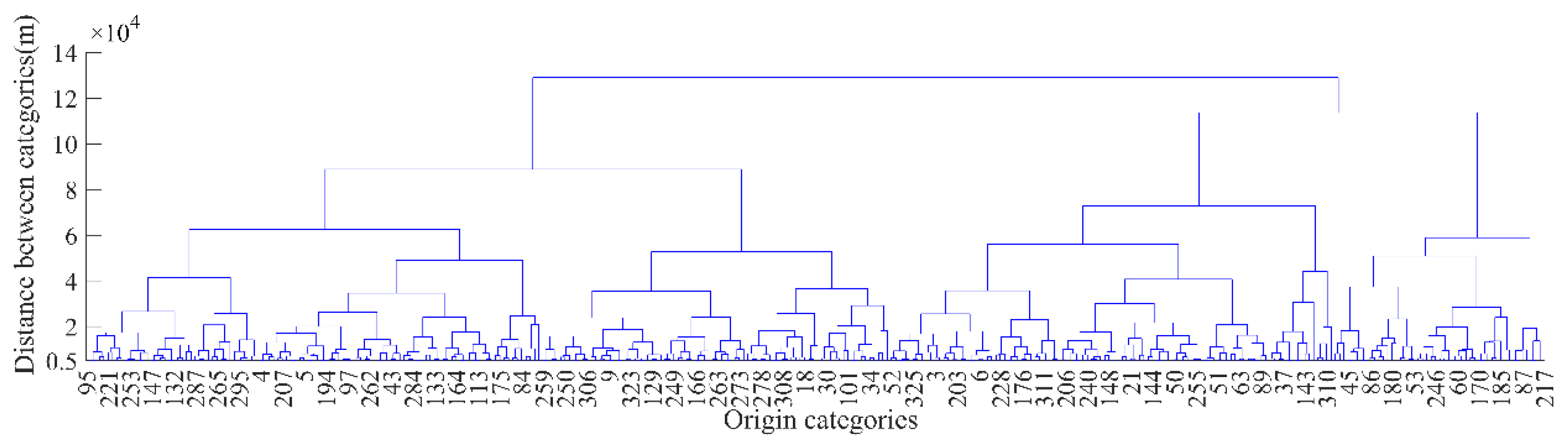
The origin areas were divided into 334 categories. The origin hierarchical clustering tree is shown in Figure 6, which illustrates the arrangement of the clusters produced by AHC. In the figure, the y-axis marks the distance at which the clusters merge, whereas the objects are placed along the x-axis so that the clusters do not mix. The nodes on the bottom of this tree represent 44,043 individual observations all plotted at zero distance (which are not shown in Figure 6), and the remaining nodes represent the clusters to which the data belong, with the vertical bar representing the distance. The distance between merged clusters is monotonous, increasing with the level of the merger. Figure 6 shows distances greater than or equal to 5000 m. The 334 origin categories’ numbers are marked in the horizontal axis. To clearly display category numbers, only the numbers of some categories are shown here.
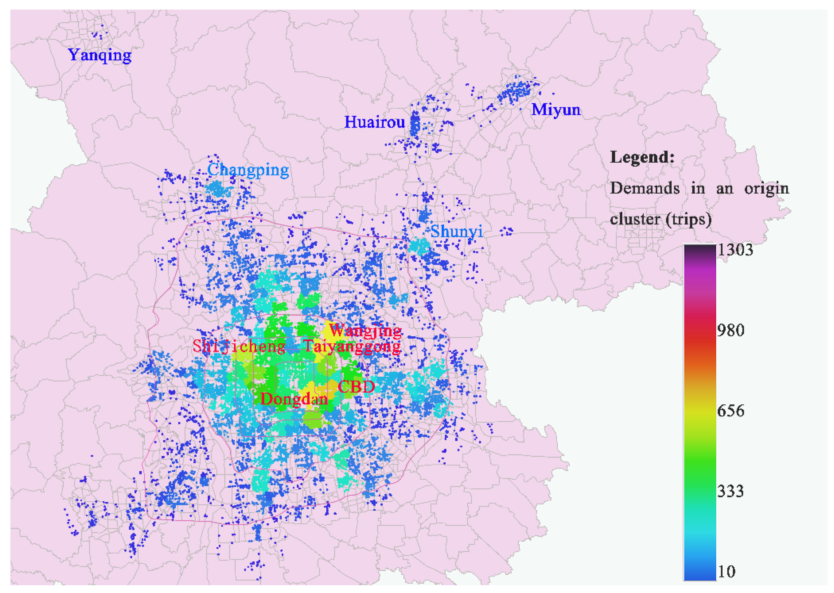
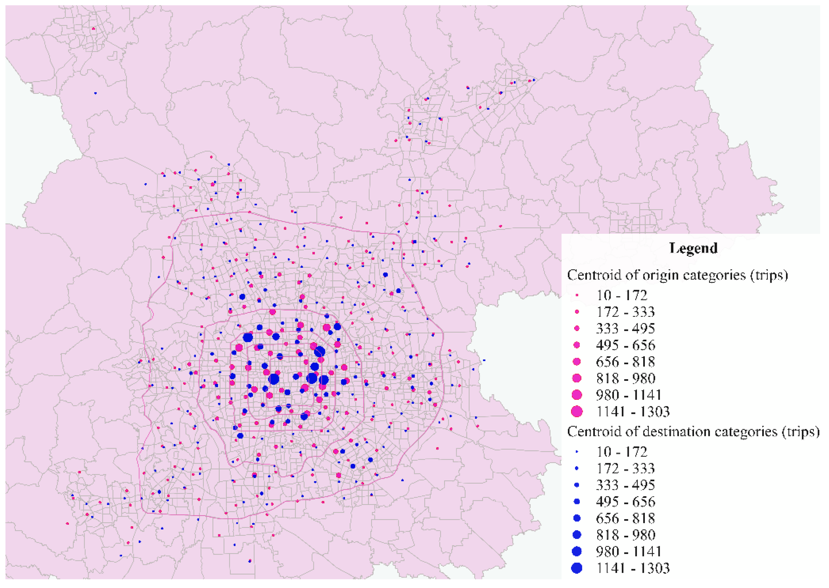
We removed the elements for which the number of elements in a cluster is less than and in which the distance from the destination to the origin centroid is less than . After screening, 267 categories were left, involving 42,563 trips, as shown in Figure 7. Among them, the five origin areas with the highest demand density are the Central Business District (CBD) (with 812 trips), Dongdan (with 779 trips), Wangjing (with 771 trips), Taiyanggong (with 744 trips), and Shijicheng (with 684 trips).
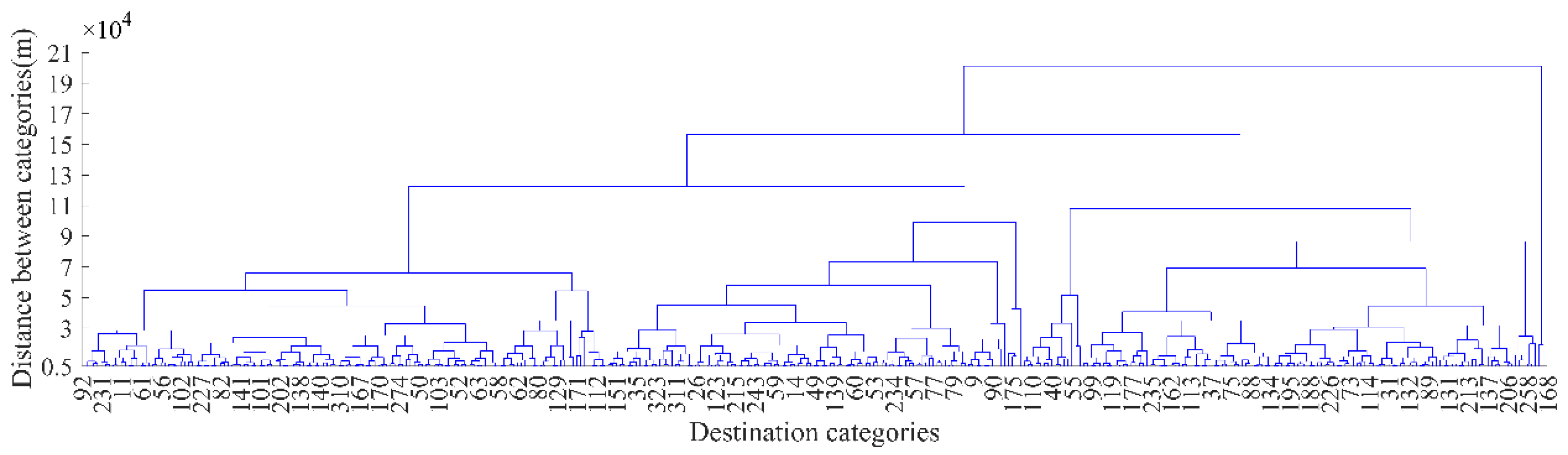
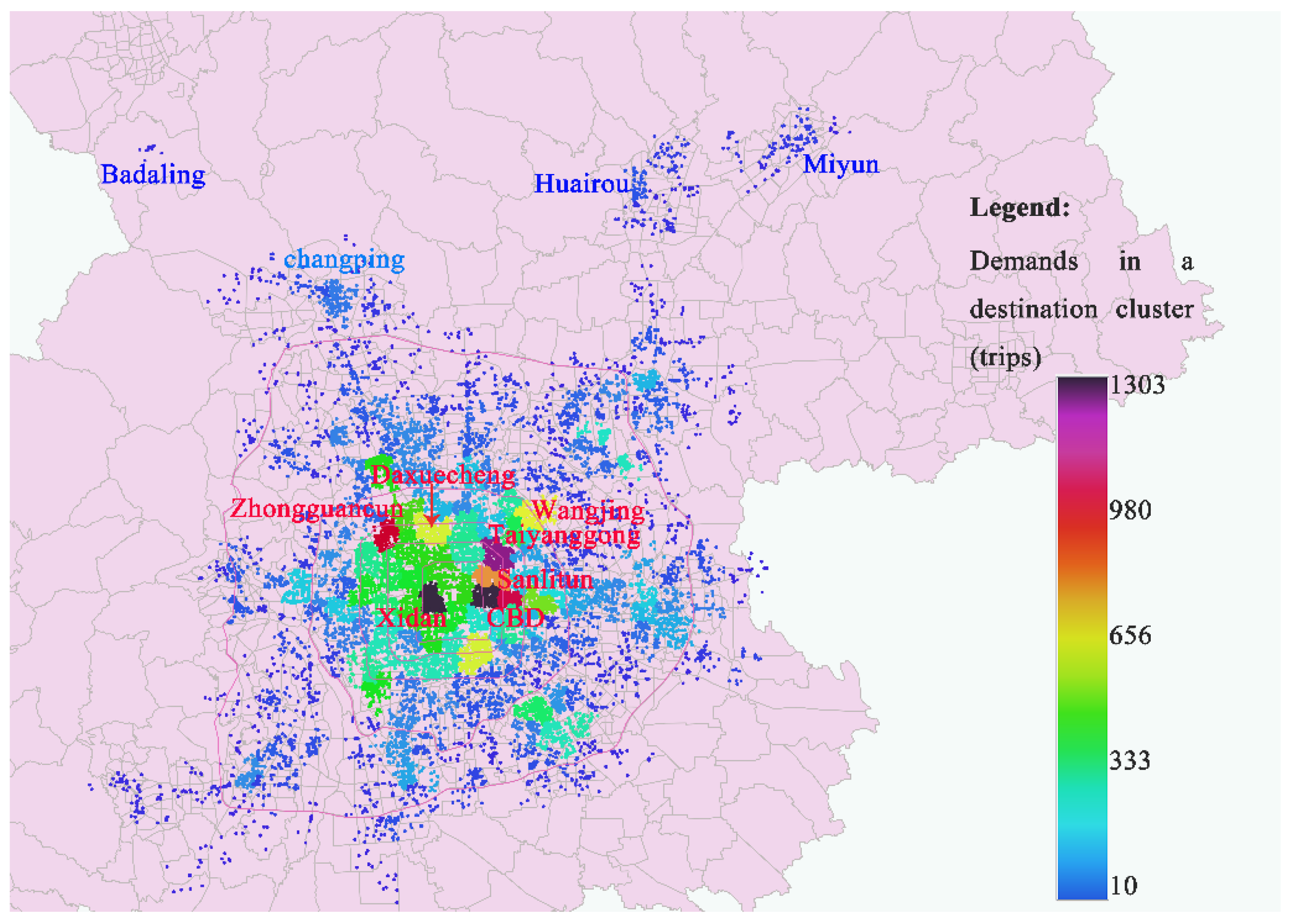
The destination areas were divided into 369 categories. The destination hierarchical cluster tree is shown in Figure 8. We removed the elements for which the number of elements in a cluster was less than . After screening, 265 categories remained, involving 42,189 trips, as shown in Figure 9. Among them, the top five destination areas in terms of demand density were Xidan (1303 trips), CBD (1300 trips), Wangjing (1213 trips), Zhongguancun (1079 trips), and Sanlitun (917 trips).
Figure 10 shows the centroid of the origin and destination categories.
3.3. Initial Line Set
Based on the results of the OD area division in Section 3.2, 70,755 lines were obtained by pairing the OD areas, which formed a set of lines to be selected. A travel OD demand table was obtained by processing the travel demand data corresponding to the 70,755 lines. To compound the actual situation, the length of a CB line was set to the average travel distance of all the demands on the line. We obtained 489 lines that would satisfy the line length constraints and the demands constraints outlined in Section 2.4.
3.4. Optimized CB Lines
The final operating scheme for the Beijing CB network was settled using MATLAB (MathWorks, USA) according to the line selection model in Section 2.5. The related parameters were as follows: the average load capacity per OCH , the fuel cost per kilometer per OCH vehicle , the fixed operating cost per OCH vehicle per day , the environmental pollution cost per unit of pollution , the pollutant emissions per OCH per kilometer , the value per unit of time , the average running speed of the bus in the case of exclusive bus lanes and traffic congestion , the average running speed of buses during normal running , the average running speed of cars during traffic congestion , the average running speed of cars during normal running , the CB fare per person per kilometer , CB fixed fare , OCH distance fare , the time fare based on time interval , the long distance fare charging , average speed of an OCH , the weight of operating cost , the weight of environmental cost , the weight of traffic congestion cost , the weight of passengers’ cost , , , and . Table 3 lists the fuel cost per kilometer per bus for CB type j, the fixed operating cost per bus per day for CB type j, and the pollutant emissions per bus per kilometer for the CB type j.
In Figure 11, Figure 12, Figure 13, Figure 14, Figure 15 and Figure 16 and Table 4, Table 5, Table 6 and Table 7, I–IV show that only one type of CB vehicle is used on each CB line, with 49, 30, 28, and 18 seats, respectively. I & IV indicate that two types of CB vehicles, with 49 and 18 seats, are used on one CB line. Similarly, I & III indicate that CB vehicles with 49 and 28 seats are operating on one CB line.
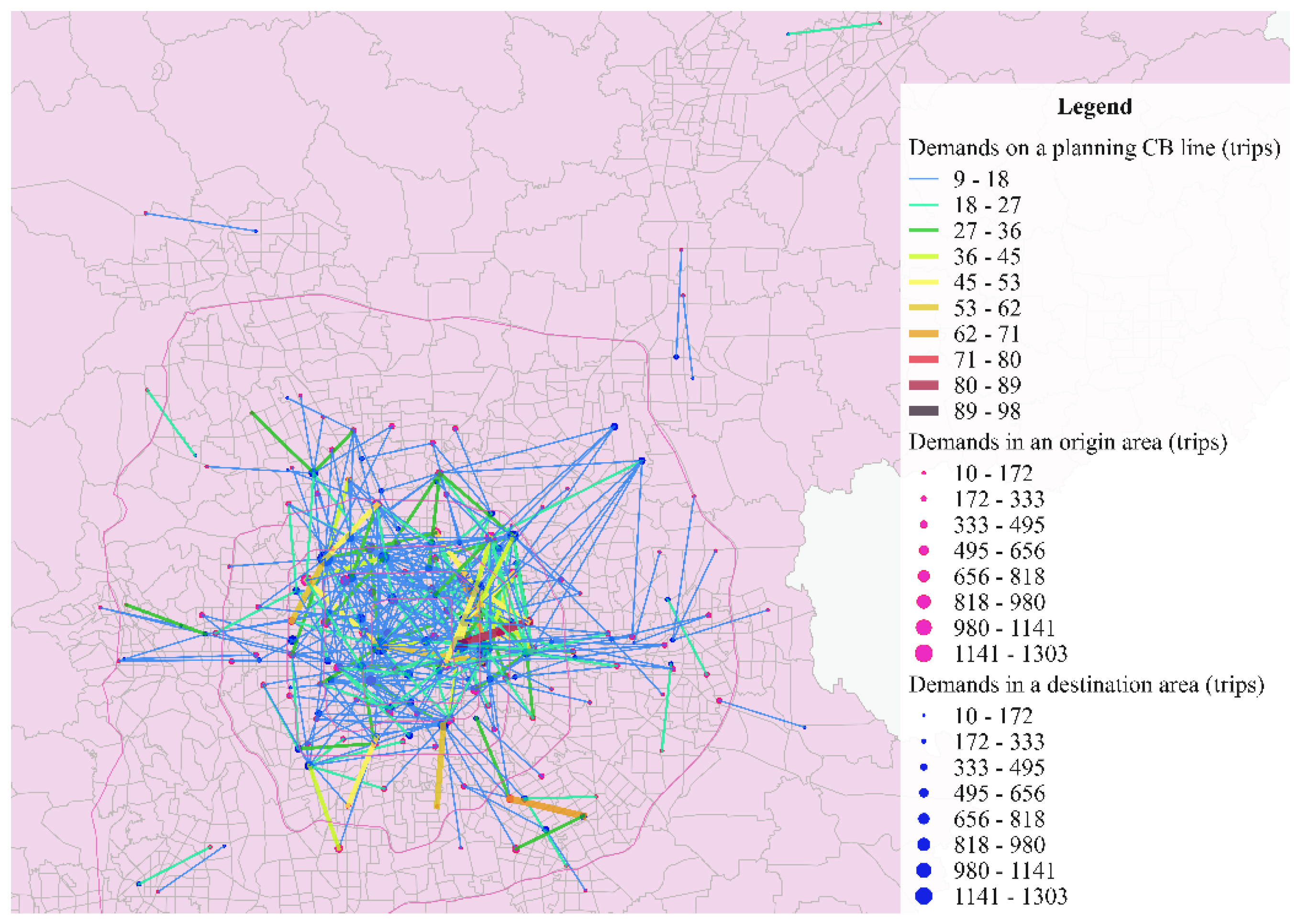
We planned 423 optimized CB lines for which a combination of two types of CB vehicles with 49 seats and 18 seats were used, as shown in Figure 11. , , , , and were set. Among them, the top six lines in terms of demands served by CB are as follows:
- From ShiQiao GuoMao Serviced Apartment to Beijing Gateway Plaza (with a total travel demand of 100 trips and CB demand for 98 trips);
- From Shifoying Dongli to Capital Institute of Pediatrics (with a total travel demand of 84 trips and CB demand of 84 trips);
- From Xibahedongli to CBD Core Area (with a total travel demand for 67 trips and CB demand for 67 trips);
- From Xinkangjiayuan to Jingdong Dasha (with a total travel demand for 64 trips and CB demand for 64 trips);
- From Linglongtiandi to Haixing Dasha (with a total travel demand for 62 trips and CB demand for 62 trips); and
- From Juyuan Beili to Shunsitiao (with total travel demands for 62 trips and CB demands for 62 trips).
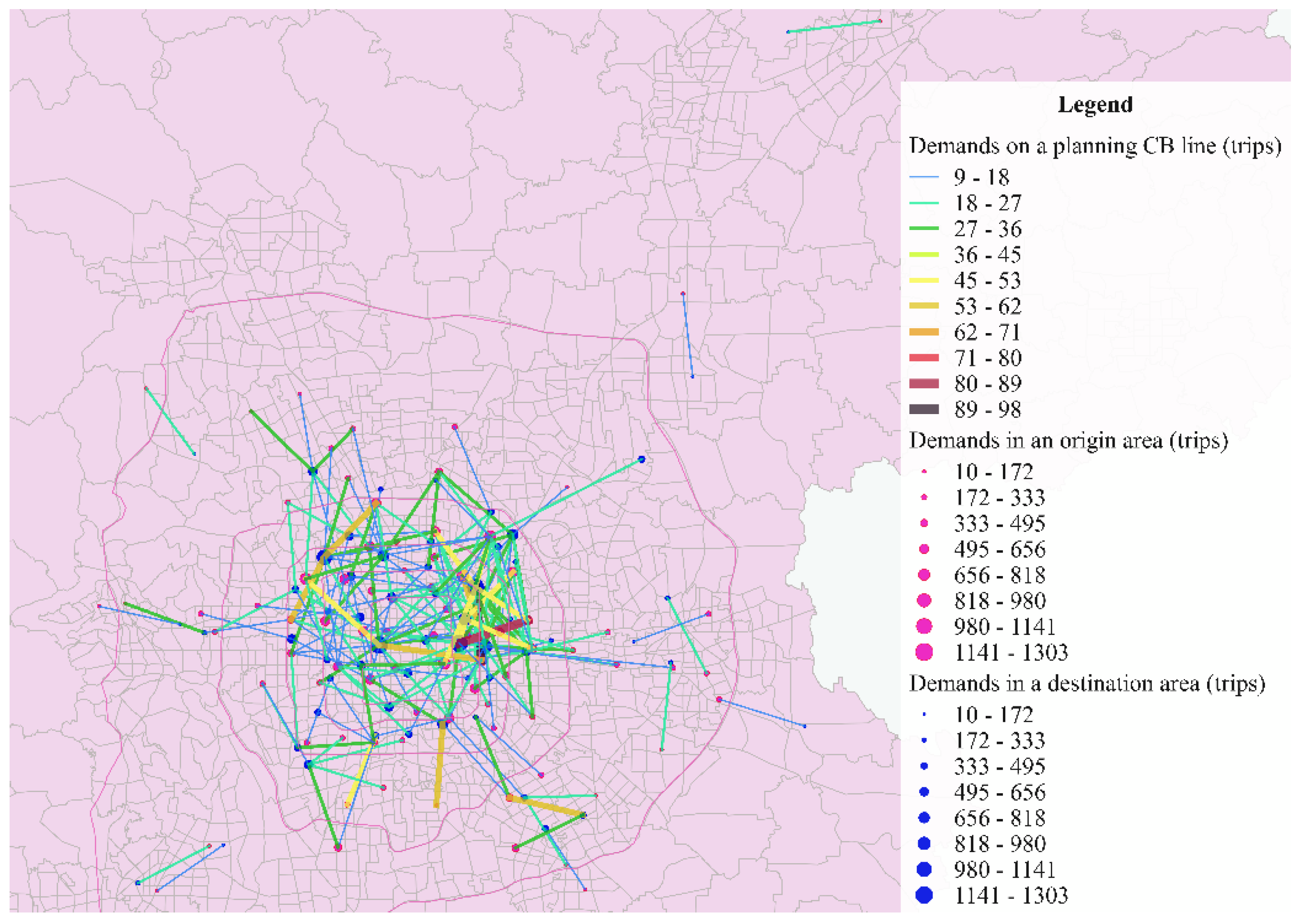
Similarly, 204 CB lines are planned when only one type of CB vehicle with 30 seats runs on each CB line, which is shown in Figure 12. Among them, the top six CB lines in terms of demands served by CB are as follows:
- From ShiQiao GuoMao Serviced Apartment to Beijing Gateway Plaza (with a travel demand for 100 trips and CB demand for 90 trips);
- From Shifoying dong li to Capital Institute of Pediatrics (with a total travel demand of 84 trips and CB demand for 84 trips);
- From Xibahedongli to CBD Core Area (with a total travel demand for 67 trips and CB demand for 60 trips);
- From Xinkangjiayuan to Jingdong Dasha (with a total travel demand for 64 trips and CB demand for 60 trips);
- From Linglongtiandi to Haixing Dasha (with a total travel demand for 62 trips and CB demand for 60 trips); and
- From Juyuan Beili to Shunsitiao (with a total travel demand for 62 trips and CB demand for 60 trips).
4. Sensitivity Analysis
4.1. Problem Statement
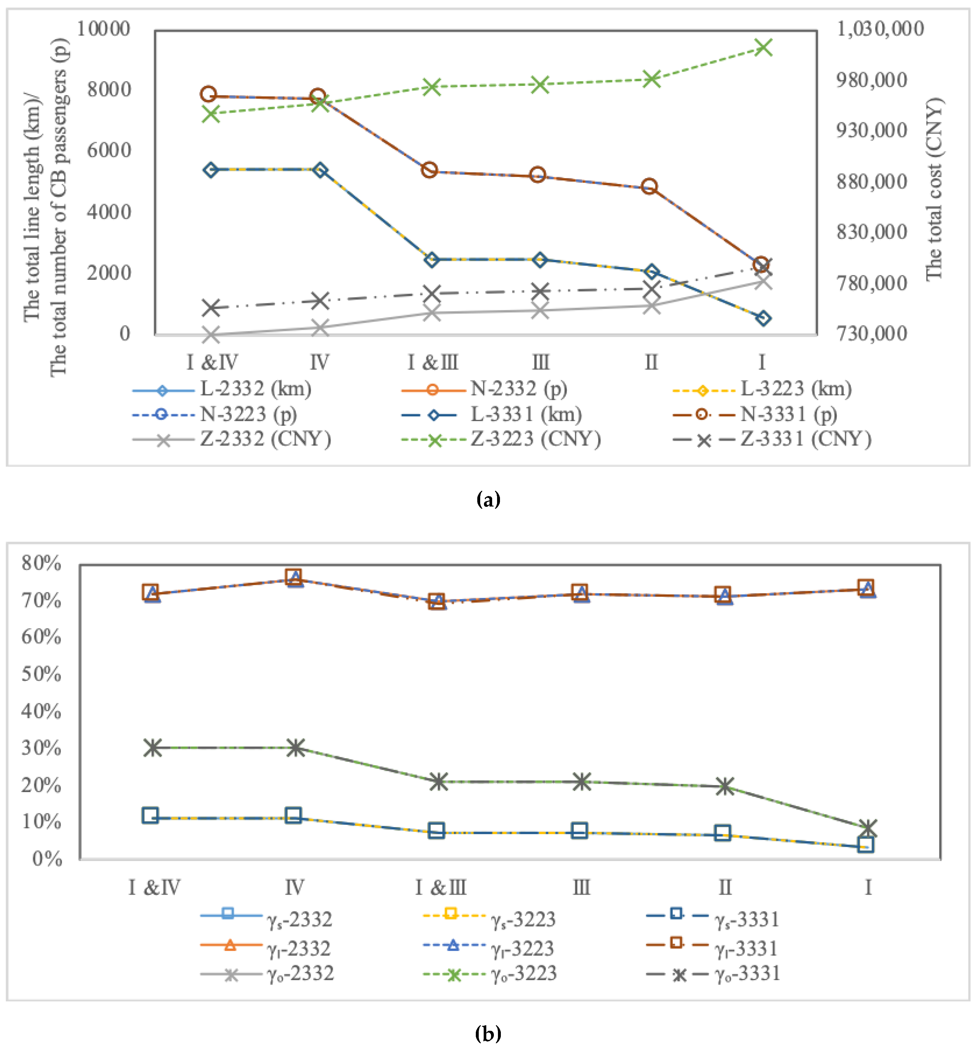
To reveal the influences of the different maximum load capacities per CB vehicle , the fixed operating cost of OCH , the weight of the operating cost , the weight of the environmental cost , the weight of the traffic congestion cost , and the weight of the cost of passengers , we analyzed the sensitivity of these parameters. represents the main investment in OCH, including the car purchase cost, insurance (full) fee, car maintenance fee, annual check-up fees, salary of the driver, etc., in different forms. For example, means that OCH vehicles are personally owned vehicles, for which the fixed operating costs are not considered in this paper. , , and denote different acquisition costs of taxi vehicles. , , and represent the proportion of the attention paid by decision-makers to each factor when CB lines are planned. For example, , , , and (abbreviated as 2332 in Table 4, Table 5, Table 6 and Table 7) mean that decision-makers pay more attention to the environmental pollution and congestion issues. Similarly, , , , and (abbreviated as 3223 in Table 4, Table 5, Table 6 and Table 7) mean that decision-makers regard operating costs and the cost of passengers as more important. , , , and (abbreviated as 3331 in Table 4, Table 5, Table 6 and Table 7) indicate that decision-makers pay more attention to operating costs, environmental pollution, and congestion issues.
4.2. The Influence of
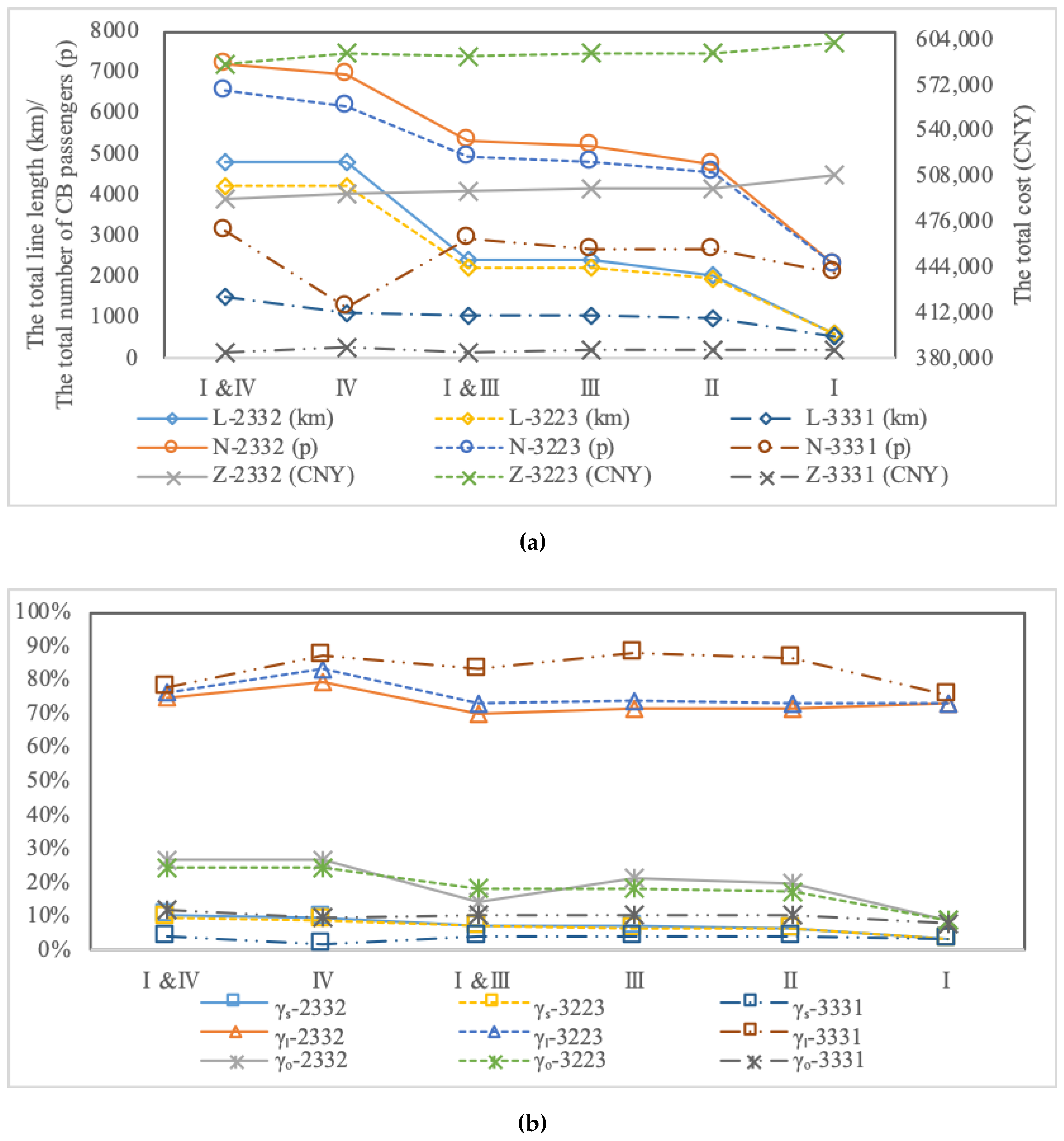
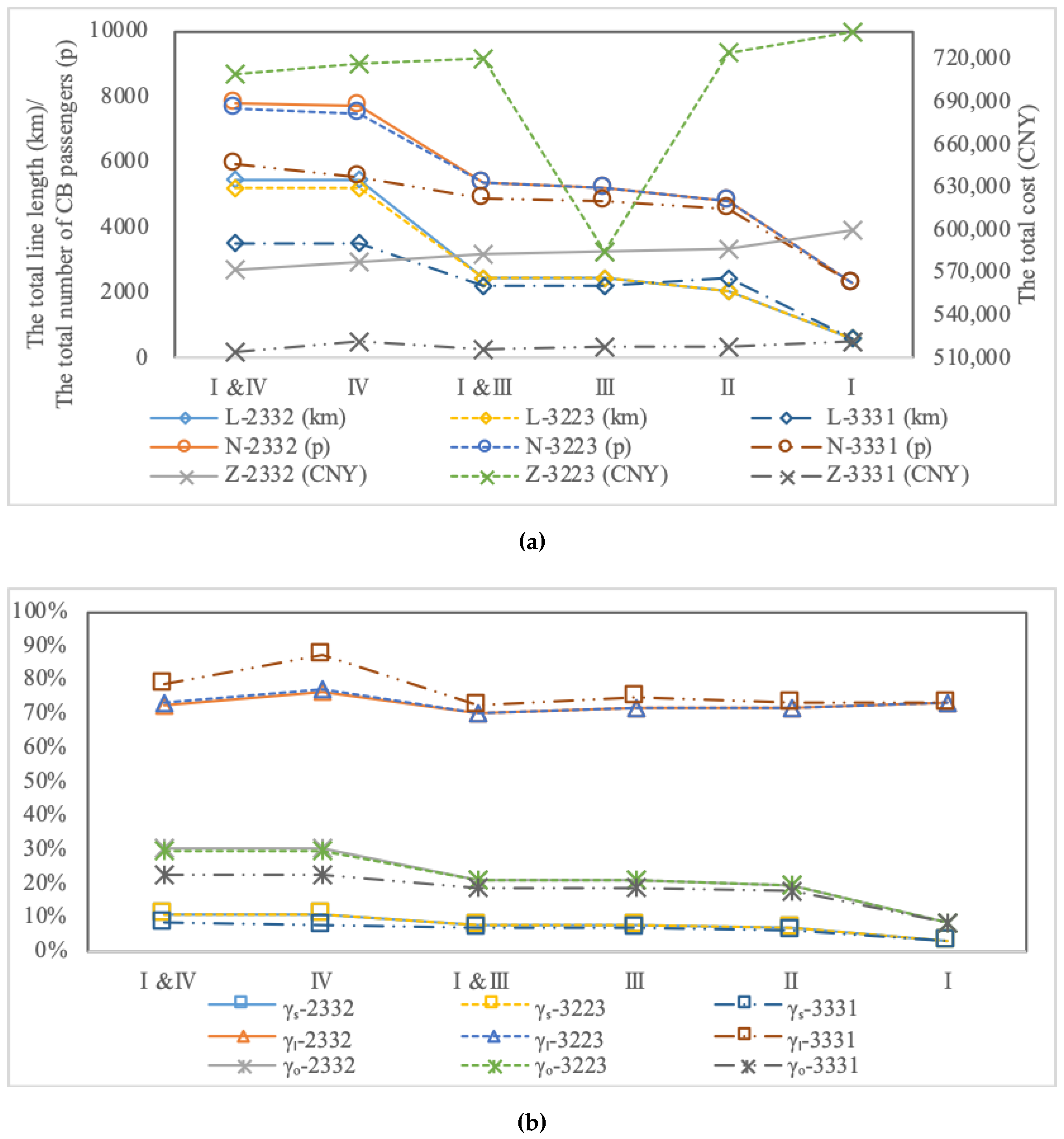
In Figure 13a, the abscissa is the operating condition related to CB vehicle type usage. The left ordinate indicates the total number of CB passengers and the total line length, and the right ordinate indicates the total cost. The abscissa in Figure 13b is consistent with that in Figure 13a. The ordinate indicates , , and .
The comparative results of the number of optimized lines, the total line length, the average line length, the number of type 1 CB vehicles, the number of type 2 CB vehicles, the total number of CB vehicles, the number of passengers served by type 1 CB vehicles, the number of passengers served by type 2 CB vehicles, and the total number of CB passengers in different scenarios when are presented in Table 4.
Combining Table 4 with Figure 13, the most cost-effective choice is to use a combination of CB vehicles with 49 seats and 18 seats (I & IV) to provide services on one CB line because they serve the most passengers at the lowest cost, and create the longest CB lines with the highest service rate, the highest site coverage rate, and the second highest average load factor. Although this combination provides the same CB line length to serve slightly fewer passengers, gaining relatively higher average load factor, equal site coverage rate, and relatively lower service rate, the cost is much higher compared with I & IV when only one type of CB vehicle with 18 seats (IV) is used. The more seats, the less cost-effective the system is when only one type of vehicle is running. Using only one type of CB vehicle with 49 seats (I) is the least cost-effective. For instance, the total CB line length, the total number of CB passengers, the total cost, the service rate, the site coverage rate, and the average load factor of I&IV are 8.32, 3.18, 0.97, 3.18, 3.15, and 1.01 times of that IV, respectively, when and decision-makers pay more attention to the environmental pollution and congestion issues.
4.3. The Influence of , , and
The CB bus lines with the longest total CB line length that serve the most CB passengers can be planned when , , , and . The highest and occur with the highest service acceptance rate and the maximum spatial coverage. The lowest occurs with the lowest vehicle use. Conversely, the CB bus lines with the shortest total CB bus line length are planned when , , , and , which serves the fewest CB passengers. The lowest and occur simultaneously, indicating the lowest service acceptance rate. This results in the highest , indicating the highest vehicle use. For instance, when , , , and , is 2.33 times that of the factor weights with , , , and , in which a combination of CB vehicles with 49 and 18 seats is used. The multiple is 5.61 when only one type of CB vehicle with 18 seats are used. When , , , and are used, is 2.28 times than when , , , and in which I & IV are used. The multiple is 2.82 when type IV is used. When , , , and , is 0.96 times and 0.91 times that of the factor weights with , , , and in which I & IV, and IV are used, respectively.
The evaluation indexes when are shown in Figure 14 and Table 5. , , and , when, , , , and are 1.32, 1.35, and 0.92 times that of when , , , and , respectively, in which I & IV are used. Similarly, these multiples are 1.40, 1.35, and 0.87 times when IV is used.
4.4. The Influence of
Figure 13, Figure 14, Figure 15 and Figure 16 show that the service rate and the site coverage rate increase with the fixed operating cost per OCH vehicle per day . The average load factor decreases as increases. For example, and increase by 11.37% and 13.76%, respectively, when increases from 0 to 30.
5. Conclusions
CB is a type of green, intensive, and innovative public transport. On the basis of meeting individual travel needs, individual motorized travel can be guided toward CB travel based on large data. Based on the features of OCH data, CB line planning methods were proposed in this paper. OCH data are active access data and provide more detail. In comparison, questionnaire data provided on the Internet [11] are passively acquired data and have fewer details.
This paper presented a detailed flow chart of CB line planning, which could effectively reduce the problem of redundant computation in the intermediate process. Then, a line selection model was established striking a balance between operator interests, social benefits, and passengers’ interests. Finally, we discussed the impacts of the CB vehicle type, the fixed operating cost of OCH and the weights of each itemized cost. Several operating schemes for the Beijing CB network were created. The results of this paper can provide technical support for CB operators who design a CB network.
Based on the results of the sensitivity analysis, the combination of CB vehicles with 49 seats and 18 seats is the most cost-effective regardless of factor values. Using the CB vehicles with 18 seats on one CB line is sensible when only one type of CB vehicle can be used. The least cost-effective arrangement is when only the CBs with 49 seats are used.
The CB network has the longest total CB line length and serves the most CB passengers with the highest service acceptance rate and the maximum spatial coverage when decision-makers pay more attention to environmental pollution and congestion issues. It also has the lowest vehicle use. Conversely, the CB network has the shortest total CB line length and serves the least CB passengers with the lowest service acceptance rate and the minimum spatial coverage when decision-makers pay more attention to operating cost, environmental pollution, and congestion issues. This scheme also has the highest vehicle use.
The CB network’s service acceptance rate and the spatial coverage increase with the fixed operating cost per OCH vehicle per day . CB vehicle use decreases as increases.
CB network planning has undergone rapid development over the last decade; much work is still to be done in this field. Many of these achievements remain to be applied in transport practice. Here, we assumed that passengers travel by either bus or car. A further refinement of the models is needed to incorporate other modes of transport. A travel mode selection model should be built in the future that can precisely mine all potential passengers of CBs. The influences of different fares on CB line planning should be discussed.
Author Contributions
Conceptualization, Z.H. and Y.C.; methodology, Z.H. and Y.C.; software, Z.H. and K.Z.; validation, Y.C.; formal analysis, Z.H.; resources, Y.C.; data curation, Y.C.; writing—original draft preparation, Z.H.; writing—review and editing, Z.H.; visualization, Z.H., H.L. and J.S.; supervision, Y.C.; project administration, Y.C.; funding acquisition, Y.C.
Funding
This study was supported by Beijing Major Science and Technology Project: Z181100003918010.
Acknowledgments
The authors thank the Beijing Transportation Information Center for providing data support in this research. We thank Yadan Yan and Dongwei Wang for their assistance with manuscript presentation. Special thanks to MDPI professional language editing services to ensure that English grammar is free of mistakes for this manuscript. Polly Wang supervised this project.
Conflicts of Interest
The authors declare that they have no conflicts of interest.
Appendix A. Sets, Indices, and Parameters
| Symbol | Definition |
| Set of origins in raw data depicted in Table 2 | |
| Set of destinations in raw data depicted in Table 2 | |
| Set of origins deleting the data whose line distance is less than | |
| Set of destinations corresponding to data set | |
| Set of origins eliminating elements that do not conform to the regulations | |
| Set of destinations eliminating elements that do not conform to the regulations | |
| Set of destinations that conform to the regulations of line length and elements | |
| U | Set of initial lines |
| Number of reservation demands | |
| Number of origin categories | |
| Number of elements in origin category , | |
| Number of elements in category | |
| Number of destination categories | |
| Number of elements in destination category , | |
| Number of demands for line i | |
| L | Number of lines that are connected by paring OD areas |
| Low limit demands in one origin area considered to be served by CB | |
| Low limit demands in one destination area considered to be served by CB | |
| Line distance of demand n between its’ origin and destination, | |
| Low limit line length considered to be served by CB | |
| Line distance between the centroid and destination of the element m in origin category , | |
| Low limit line distance between the centroid of origin category and the corresponding destinations | |
| Line length of line i | |
| Minimum line length | |
| Total operating cost on line i, | |
| Fuel cost per kilometer per bus for the CB type j, | |
| Ω | Number of CB vehicle types which have different maximum load capacities |
| Number of vehicles for the CB type j on line i | |
| Mileage on the line i | |
| Fixed operating cost per bus per day for the CB type j | |
| Fuel cost per kilometer per car for OCH | |
| Number of vehicles for OCH on line i | |
| Fixed operating cost per OCH vehicle per day | |
| Total environmental pollution cost on line i | |
| Environmental pollution cost per unit of pollution | |
| Pollutant emissions per bus per kilometer for the CB type j | |
| Pollutant emissions per OCH per kilometer | |
| The total congestion cost on line i | |
| Value per unit of time | |
| Average running speed of the bus in the case of exclusive bus lanes and traffic congestion | |
| Average running speed of buses during normal running | |
| Number of people travelling by CBs on line i | |
| Average running speed of cars in the case of traffic congestion | |
| Average running speed of cars during normal running | |
| Number of people travelling by OCH on line i | |
| v | Average speed of OCH |
| Total cost of tickets on line i | |
| CB fare per person per kilometer charging for distances above | |
| CB fixed fare charging for the distance within (including ) | |
| Mileage boundary of CB for changes in fare rates | |
| Mileage boundary of OCH for changes in fare rates | |
| Minimum fare | |
| OCH distance fare | |
| Time fare based on time interval | |
| Long distance fare charging for the distance above 20 km | |
| Total cost of line i | |
| Operating cost weight | |
| Environmental cost weight | |
| Traffic congestion cost weight | |
| Cost weight of fares paid by passengers | |
| Number of people traveling by CB vehicle of type j on each line | |
| Maximum load capacities per CB vehicle of type j | |
| Travel distance of passengers on each line | |
| Total travel demand on each line | |
| Average load capacity per OCH | |
| Total line length when , , , and | |
| Total number of CB passengers when , , , and | |
| The total cost when , , , and | |
| . | Total line length when , , , and |
| Total number of CB passengers when , , , and | |
| Total cost when , , , and | |
| Total line length when , , , and | |
| The total number of CB passengers when , , , and | |
| . | Total cost when , . , , and |
| The service rate when , , , and | |
| Average load factor when , , , and | |
| The site coverage rate when , , , and | |
| Service rate when , , , and | |
| Average load factor when , , , and | |
| Site coverage rate when , , , and | |
| Service rate when , , , and | |
| Average load factor when , , , and | |
| Site coverage rate when , , , and |
References
- Dias, F.F.; Lavieri, P.S.; Kim, T.; Bhat, C.R.; Pendyala, R.M. Fusing Multiple Sources of Data to Understand Ride-Hailing Use. Transp. Res. Rec. 2019, 2673, 214–224. [Google Scholar] [CrossRef]
- Jain, S.; Ronald, N.; Thompson, R.; Winter, S. Predicting susceptibility to use demand responsive transport using demographic and trip characteristics of the population. Travel Behav. Soc. 2017, 6, 44–56. [Google Scholar] [CrossRef]
- Lyu, Y.; Chow, C.Y.; Lee, V.; Ng, J.; Li, Y.H.; Zeng, J. CB-Planner: A bus line planning framework for customized bus systems. Transp. Res. C-Emer. 2019, 101, 233–253. [Google Scholar] [CrossRef]
- Amirgholy, M.; Gonzales, E.J. Demand responsive transit systems with time-dependent demand: User equilibrium, system optimum, and management strategy. Transp. Res. B-Meth. 2016, 92, 234–252. [Google Scholar] [CrossRef]
- Shen, J.; Yang, S.; Gao, X.; Qiu, F. Vehicle routing and scheduling of demand-responsive connector with on-demand stations. Adv. Mech. Eng. 2017, 9. [Google Scholar] [CrossRef]
- Chen, P.W.; Nie, Y.M. Analysis of an idealized system of demand adaptive paired-line hybrid transit. Transp. Res. B-Meth. 2017, 102, 38–54. [Google Scholar] [CrossRef]
- Liu, T.; Ceder, A.A. Analysis of a new public-transport-service concept: Customized bus in China. Transp. Policy 2015, 39, 63–76. [Google Scholar] [CrossRef]
- Guo, R.G.; Guan, W.; Zhang, W.Y. Route Design Problem of Customized Buses: Mixed Integer Programming Model and Case Study. J. Transp. Eng. A-Syst. 2018, 144. [Google Scholar] [CrossRef]
- Li, Y.; Yan, X.; Shao, W. Scheduling Optimization Method of Single-line Customized Bus. In Proceedings of the 2nd International Conference on Mechanical, Electronic, Control and Automation Engineering, Qingdao, China, 30–31 March 2018. [Google Scholar]
- Tong, L.; Zhou, L.S.; Liu, J.T.; Zhou, X.S. Customized bus service design for jointly optimizing passenger-to-vehicle assignment and vehicle routing. Transp. Res. C-Emer. 2017, 85, 451–475. [Google Scholar] [CrossRef]
- Ma, J.; Yang, Y.; Guan, W.; Wang, F.; Liu, T.; Tu, W.; Song, C. Large-Scale Demand Driven Design of a Customized Bus Network: A Methodological Framework and Beijing Case Study. J. Adv. Transp. 2017, 2017. [Google Scholar] [CrossRef]
- Li, J.; Lv, Y.; Ma, J.; Ouyang, Q. Methodology for Extracting Potential Customized Bus Routes Based on Bus Smart Card Data. Energies 2018, 11, 2224. [Google Scholar] [CrossRef]
- Ma, J.H.; Zhao, Y.Q.; Yang, Y.; Liu, T.; Guan, W.; Wang, J.; Song, C.Y. A Model for the Stop Planning and Timetables of Customized Buses. Plos ONE 2017, 12. [Google Scholar] [CrossRef] [PubMed]
- Li, Z.; Song, R.; He, S.; Bi, M. Methodology of mixed load customized bus lines and adjustment based on time windows. Plos ONE 2018, 13. [Google Scholar] [CrossRef] [PubMed]
- Lyu, Y.; Chow, C.; Lee, V.C.S.; Li, Y.; Zeng, J. T2CBS: Mining Taxi Trajectories for Customized Bus Systems. Comput. Commun. Workshops IEEE 2016, 441–446. [Google Scholar] [CrossRef]
- Zhang, M.; Liu, J.; Liu, Y.; Hu, Z.; Yi, L. Recommending Pick-up Points for Taxi-drivers based on Spatio-temporal Clustering. In Proceedings of the 2nd International Conference on Cloud and Green Computing/2nd International Conference on Social Computing and its Applications (CGC/SCA), Xiangtan, China, 1–3 November 2012. [Google Scholar]
- Zhu, W.; Lu, J.; Li, Y.; Yang, Y. A Pick-Up Points Recommendation System for Ridesourcing Service. Sustainability 2019, 11, 1097. [Google Scholar] [CrossRef]
- Zhao, P.; Liu, X.; Shen, J.; Chen, M. A network distance and graph-partitioning-based clustering method for improving the accuracy of urban hotspot detection. Geocarto Int. 2019, 34, 293–315. [Google Scholar] [CrossRef]
- Hu, X.; An, S.; Wang, J. Taxi Driver’s Operation Behavior and Passengers’ Demand Analysis Based on GPS Data. J. Adv. Transp. 2018, 2018. [Google Scholar] [CrossRef]
- Ma, Q.; Yang, H.; Zhang, H.; Xie, K.; Wang, Z. Modeling and Analysis of Daily Driving Patterns of Taxis in Reshuffled Ride-Hailing Service Market. J. Transp. Eng. A-Syst. 2019, 145. [Google Scholar] [CrossRef]
- Liu, Y.; Bansal, P.; Daziano, R.; Samaranayake, S. A framework to integrate mode choice in the design of mobility-on-demand systems. Transp. Res. C-Emer. 2019, 105, 648–665. [Google Scholar] [CrossRef]
- Wang, D.; Cao, W.; Li, J.; Ye, J. DeepSD: Supply-Demand Prediction for Online Car-hailing Services Using Deep Neural Networks. In Proceedings of the 2017 IEEE 33rd International Conference on Data Engineering (ICDE), San Diego, CA, USA, 19–22 April 2017. [Google Scholar]
- Jiang, S.; Chen, W.; Li, Z.; Yu, H. Short-Term Demand Prediction Method for Online Car-Hailing Services Based on a Least Squares Support Vector Machine. IEEE Access 2019, 7, 11882–11891. [Google Scholar] [CrossRef]
- Lim, E.; Hwang, H. The Selection of Vertiport Location for On-Demand Mobility and Its Application to Seoul Metro Area. Int. J. Aeronaut. Space 2019, 20, 260–272. [Google Scholar] [CrossRef]
- Zhen, H.; Liu, J.; Bing, H. Analysis of Passenger Travel Behavior Based on Public Transportation OD Data. In Proceedings of the 2018 6th International Conference On Information and Education Technology (ICIET 2018), Osaka, Japan, 6–8 January 2018. [Google Scholar]
- Luo, H.; Chen, D.; Xiong, Z.; Wang, K. Research on Trip Hotspot Discovery Algorithm Based on Hierarchical Clustering. In Proceedings of the 6th International Conference on Energy and Environmental Protection (ICEEP), Zhuhai, China, 29–30 June 2017. [Google Scholar]
- Pusadan, M.Y.; Buliali, J.L.; Ginardi, R.V.H. Anomaly Detection of Flight Routes Through Optimal Waypoint. In Proceedings of the 1st International Conference on Computing and Applied Informatics (ICCAI) - Applied Informatics Toward Smart Environment, People, and Society, Medan, Indonesia, 14–15 December 2016. [Google Scholar]
- Cluster Analysis. Available online: http://wikipedia.moesalih.com/Cluster_analysis#Definition (accessed on 23 August 2019).
- Hierarchical Clustering. Available online: http://wikipedia.moesalih.com/Hierarchical_clustering (accessed on 23 August 2019).
Figure 1.
Framework of CB network planning. Note: origin–destination (OD).
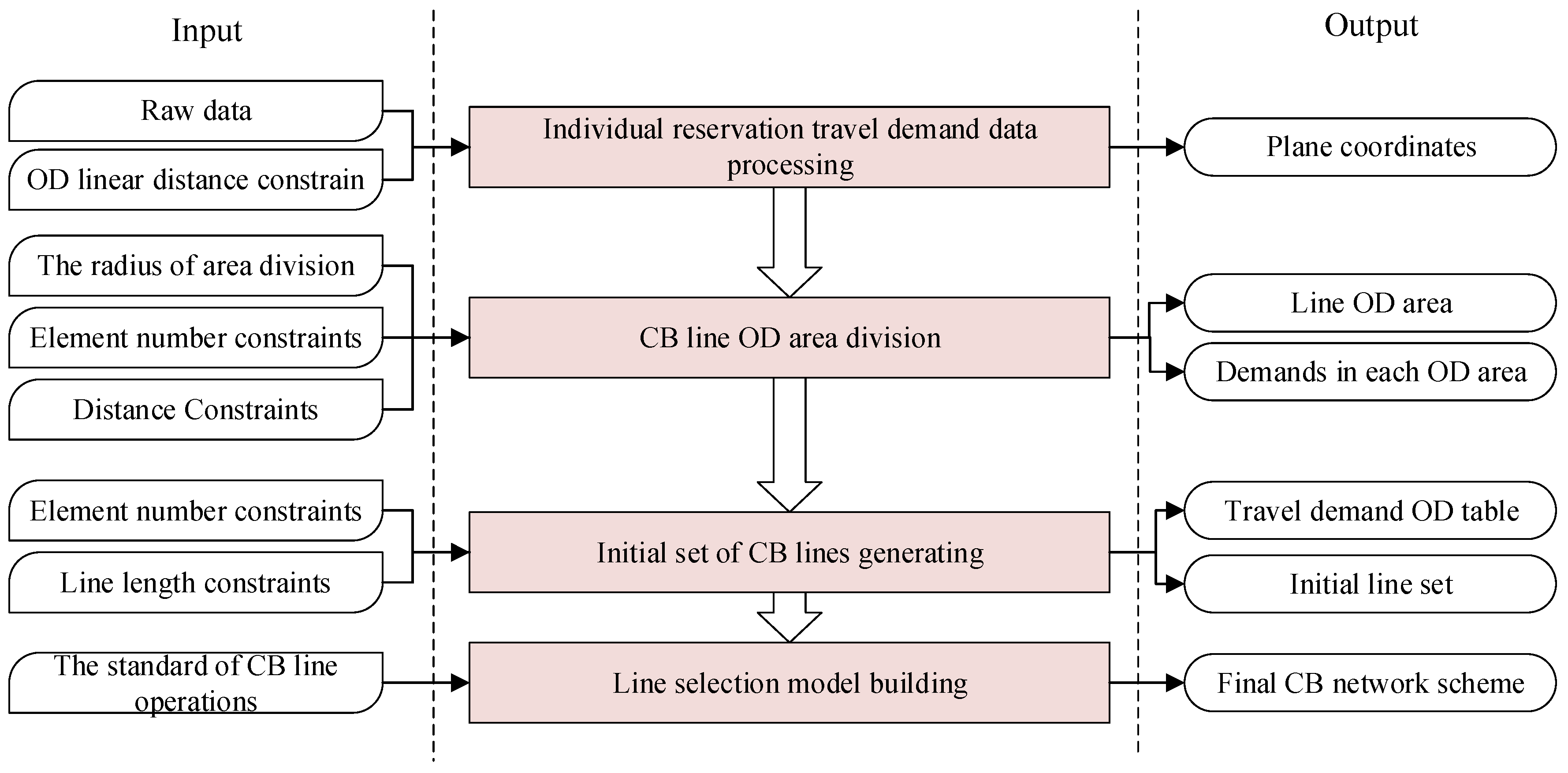
Figure 2.
Process for individual reservation travel demand data processing.
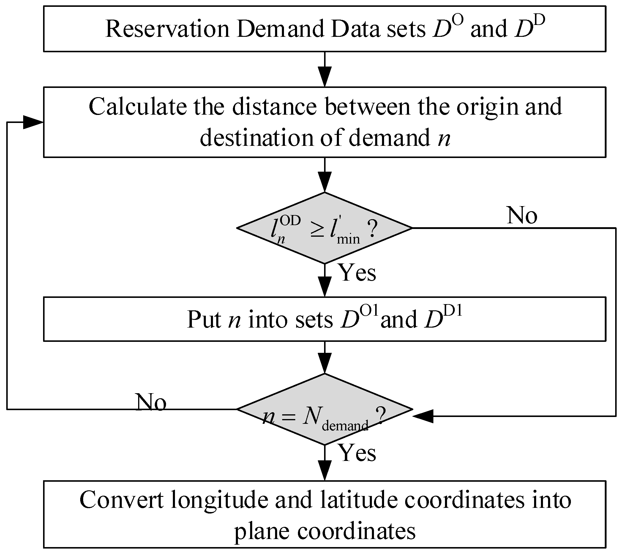
Figure 3.
Process for CB line OD area division.

Figure 4.
Process for generating the initial set of CB lines.
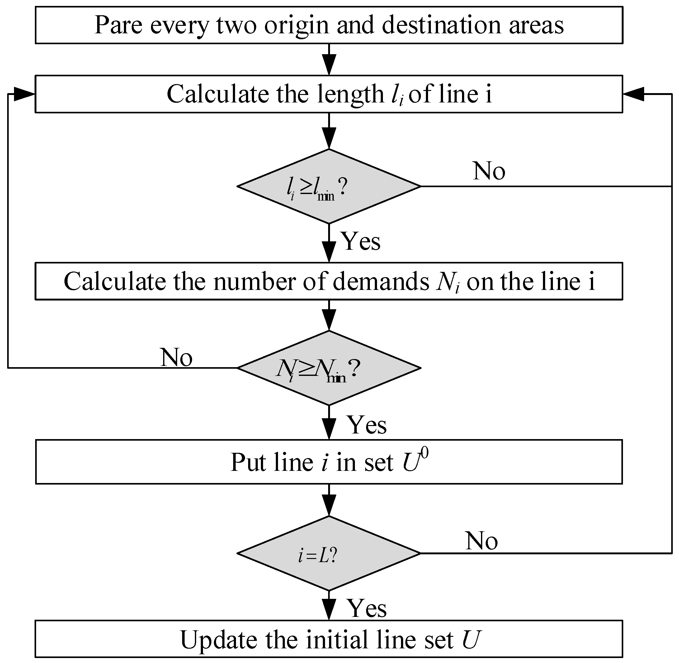
Figure 5.
Reservation demands’ time variation throughout 24 July 2017 (Monday).
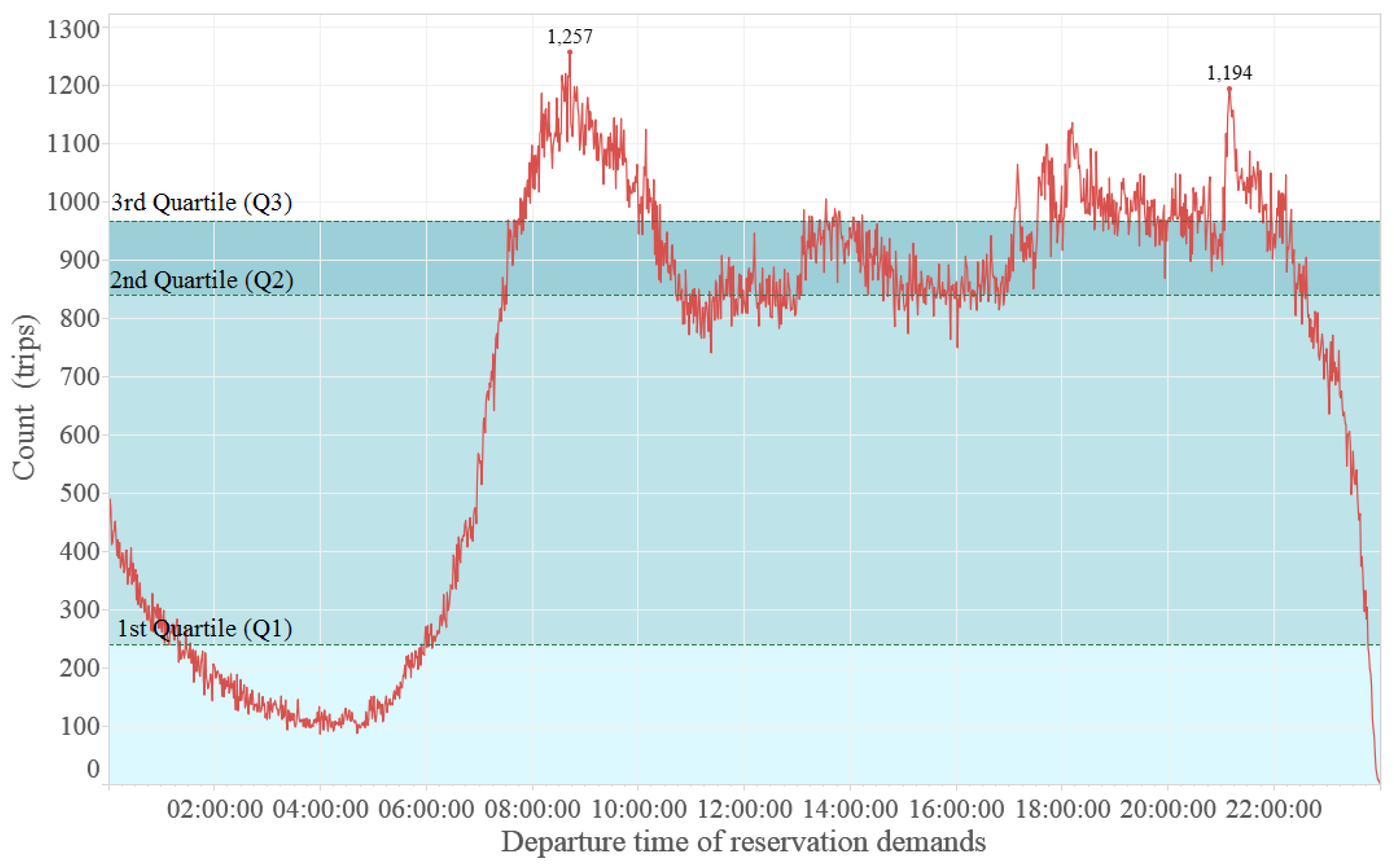
Figure 6.
Origin hierarchical clustering tree.

Figure 7.
Origin hierarchical clustering diagram.

Figure 8.
Destination hierarchical clustering tree.

Figure 9.
Destination hierarchical clustering.

Figure 10.
Cluster center distribution of origins and destinations.

Figure 11.
CB lines using I & IV when , , , , and .

Figure 12.
CB lines using II when , , , , and .

Figure 13.
Evaluation indexes when . (a) The total line length, the total number of CB passengers, and the total cost. Note: p is short for people. (b) The service rate, average load factor, and site coverage rate.
Figure 13.
Evaluation indexes when . (a) The total line length, the total number of CB passengers, and the total cost. Note: p is short for people. (b) The service rate, average load factor, and site coverage rate.

Figure 14.
Evaluation indexes when . (a) The total line length, the total number of CB passengers, and the total cost. Note: p is short for people. (b) The service rate, average load factor, and site coverage rate.
Figure 14.
Evaluation indexes when . (a) The total line length, the total number of CB passengers, and the total cost. Note: p is short for people. (b) The service rate, average load factor, and site coverage rate.

Figure 15.
Evaluation indexes when . (a) The total line length, the total number of CB passengers, and the total cost. Note: p is short for people. (b) The service rate, average load factor, and site coverage rate.
Figure 15.
Evaluation indexes when . (a) The total line length, the total number of CB passengers, and the total cost. Note: p is short for people. (b) The service rate, average load factor, and site coverage rate.
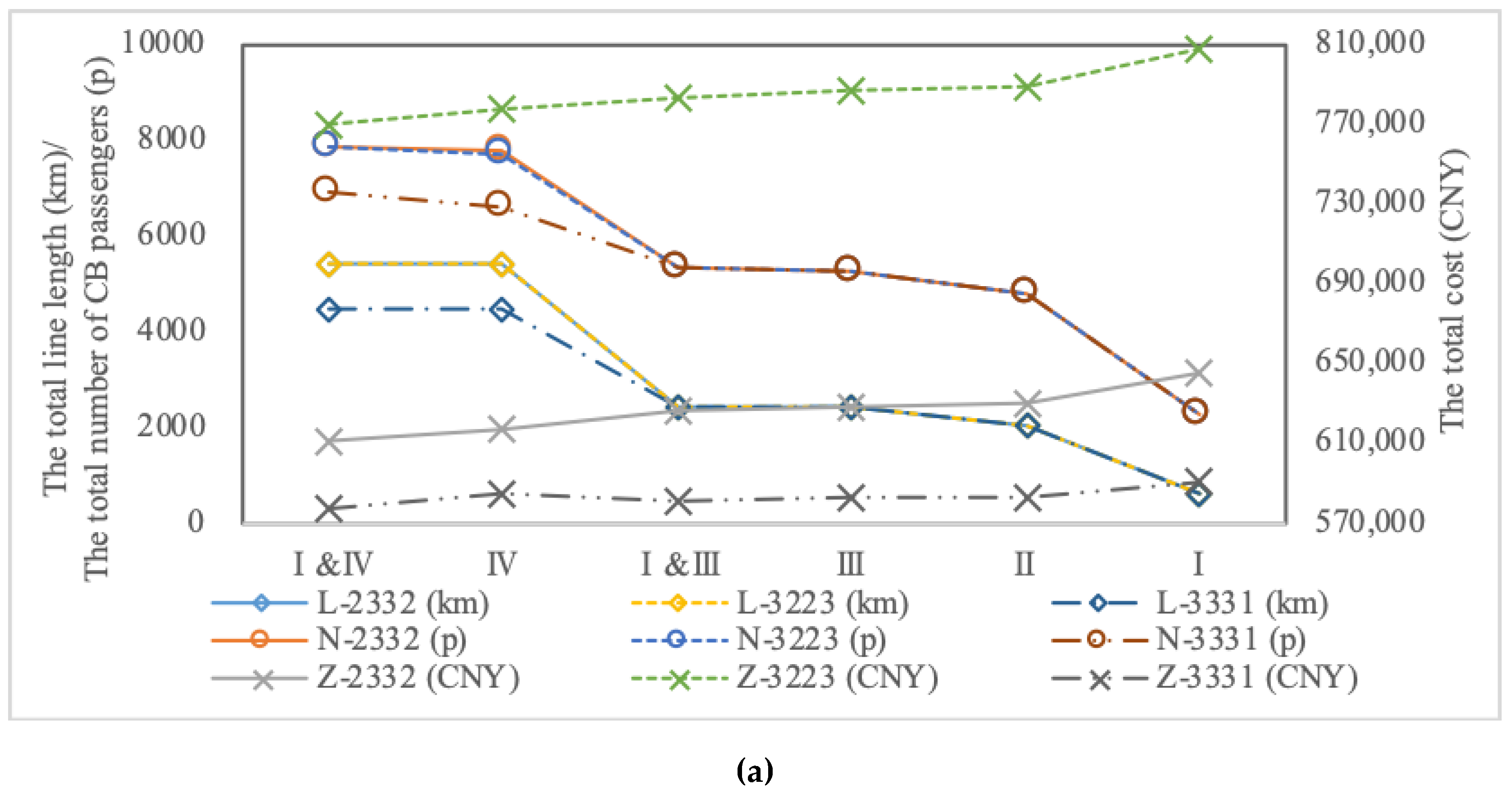
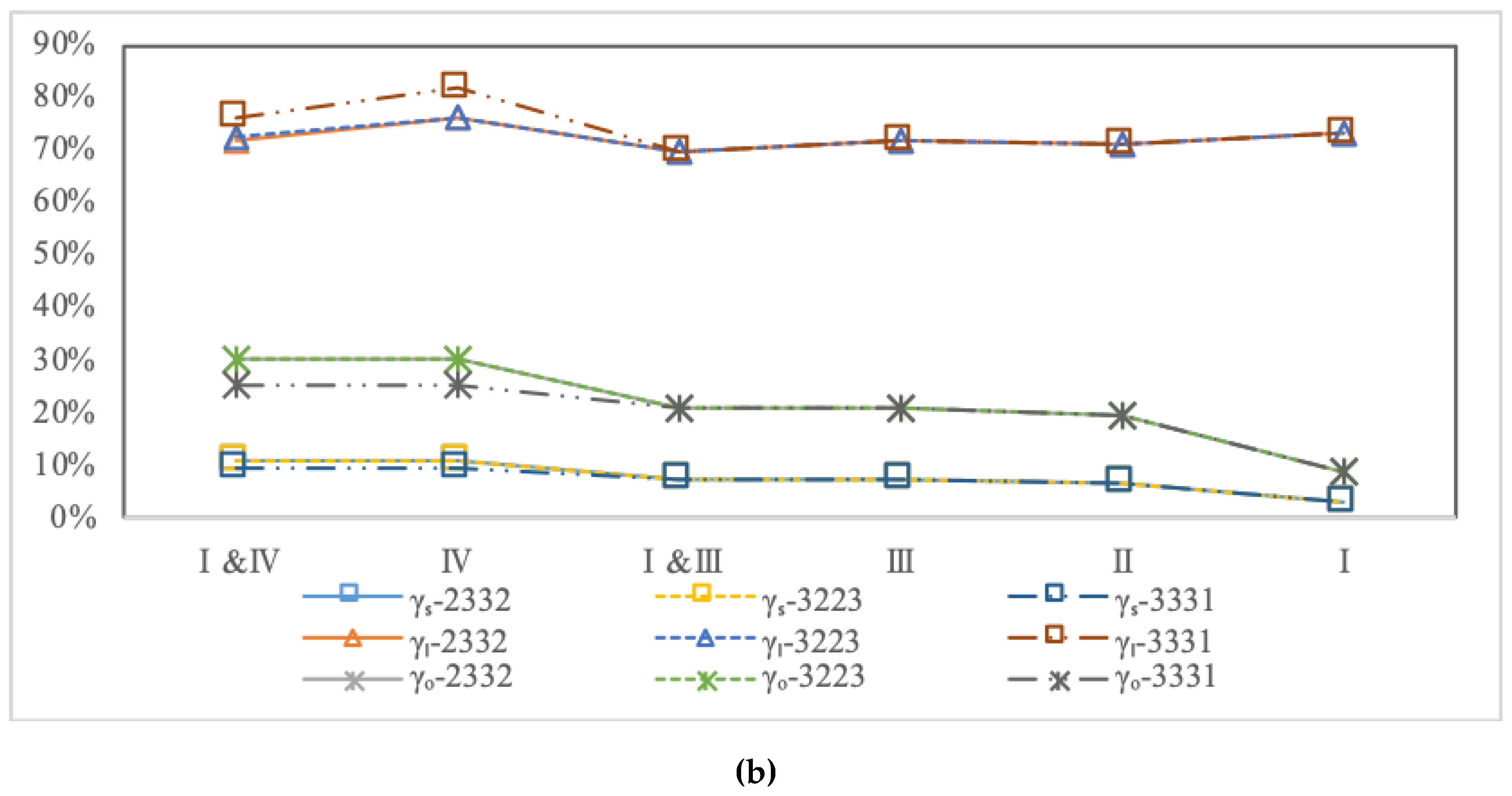
Figure 16.
Evaluation indexes when . (a) The total line length, the total number of CB passengers and the total cost. Note: p is short for people. (b) The service rate, average load factor, and site coverage rate.
Figure 16.
Evaluation indexes when . (a) The total line length, the total number of CB passengers and the total cost. Note: p is short for people. (b) The service rate, average load factor, and site coverage rate.

Table 1.
Comparison of a customized bus (CB) with online car-hailing (OCH) and conventional buses.
| CB VS. OCH | CB VS. Conventional Bus | ||
|---|---|---|---|
| Common Points | Advantages of CB | Common Points | Advantages of CB |
|
|
|
|
Table 2.
Description of data used in this study.
| Fieldname | Definition | Data Type |
|---|---|---|
| ORDER_NO | Order number | Varchar |
| DEST_VEH_LON | Longitude of real vehicle arrival site | Number |
| DEST_VEH_LAT | Latitude of real vehicle arrival site | Number |
| ON_TIME | Actual boarding time | Date |
| OFF_TIME | Actual disembarkation time | Date |
| PASSENGER_MIL | Passenger miles | Number |
| RECEIVABLE | Receivable amount | Number |
| REAL_VEHICLE_LON | Longitude of the actual departure point of the vehicle | Number |
| REAL_VEHICLE_LAT | Latitude of the actual departure point of the vehicle | Number |
Table 3.
Parameters for CB buses with different maximum load capacities per CB vehicle.
| Parameters | ||||
|---|---|---|---|---|
| 1.64 | 0.97 | 0.97 | 0.88 | |
| 449 | 396 | 396 | 360 | |
| 1.3 | 1.2 | 1.2 | 1.0 |
Table 4.
Evaluation indexes of CB lines, vehicles, and passengers when .
| Weights | CB Vehicle Types | Number of Optimized Lines | Average Line Length (km) | Number of Type 1 CB Vehicles (Bus) | Number of Type 2 CB Vehicles (Bus) | Total Number of CB Vehicles (Bus) | Number of Passengers Served by Type 1 CB Vehicles | Number of Passengers Served by Type 2 CB Vehicles |
|---|---|---|---|---|---|---|---|---|
| 2332 | I & IV | 423 | 11.41 | 63 | 367 | 430 | 2262 | 4940 |
| IV | 423 | 11.41 | - | - | 485 | - | - | |
| I & III | 237 | 10.27 | 37 | 205 | 242 | 1526 | 3785 | |
| III | 237 | 10.27 | - | - | 259 | - | - | |
| II | 204 | 10.05 | - | - | 222 | - | - | |
| I | 61 | 9.51 | - | - | 63 | - | - | |
| 3223 | I & IV | 362 | 11.64 | 63 | 306 | 369 | 2262 | 4278 |
| I & III | 211 | 10.48 | 33 | 183 | 216 | 1400 | 3517 | |
| IV | 362 | 11.64 | - | - | 411 | - | - | |
| III | 211 | 10.48 | - | - | 232 | - | - | |
| II | 190 | 10.18 | - | - | 207 | - | - | |
| I | 61 | 9.51 | - | - | 63 | - | - | |
| 3311 | I & III | 97 | 10.90 | 34 | 67 | 101 | 1449 | 1509 |
| I & IV | 116 | 12.79 | 57 | 66 | 123 | 2105 | 986 | |
| I | 55 | 9.62 | - | - | 57 | - | - | |
| II | 93 | 10.62 | - | - | 103 | - | - | |
| III | 97 | 10.90 | - | - | 108 | - | - | |
| IV | 76 | 14.82 | - | - | 79 | - | - |
Table 5.
Evaluation indexes for CB lines, vehicles, and passengers when .
| Weights | CB Vehicle Types | Number of Optimized Lines | Average Line Length (km) | Number of Type 1 CB Vehicles (Bus) | Number of Type 2 CB Vehicles (Bus) | Total Number of CB Vehicles (Bus) | Number of Passengers Served by Type 1 CB Vehicles (People) | Number of Passengers Served by Type 2 CB Vehicles (People) |
|---|---|---|---|---|---|---|---|---|
| 2332 | I & IV | 486 | 11.12 | 63 | 430 | 493 | 2262 | 5551 |
| IV | 486 | 11.12 | - | - | 562 | - | - | |
| I & III | 238 | 10.26 | 37 | 208 | 245 | 1490 | 3855 | |
| III | 238 | 10.26 | - | - | 260 | - | - | |
| II | 204 | 10.05 | - | - | 222 | - | - | |
| I | 61 | 9.51 | - | - | 63 | - | - | |
| 3223 | III | 238 | 10.26 | - | - | 260 | - | - |
| I & IV | 466 | 11.23 | 63 | 410 | 473 | 2262 | 5364 | |
| IV | 466 | 11.23 | - | - | 534 | - | - | |
| I & III | 238 | 10.26 | 36 | 209 | 245 | 1459 | 3883 | |
| II | 204 | 10.05 | - | - | 222 | - | - | |
| I | 61 | 9.51 | - | - | 63 | - | - | |
| 3331 | I & IV | 302 | 11.53 | 63 | 246 | 309 | 2262 | 3651 |
| I & III | 208 | 10.49 | 40 | 172 | 212 | 1637 | 3251 | |
| II | 190 | 10.26 | - | - | 207 | - | - | |
| III | 208 | 10.49 | - | - | 229 | - | - | |
| IV | 302 | 11.53 | - | - | 349 | - | - | |
| I | 61 | 9.51 | - | - | 63 | - | - |
Table 6.
Evaluation indexes for CB lines, vehicles, and passengers when .
| Weights | CB Vehicle Types | Number of Optimized Lines | Average Line Length (km) | Number of Type 1 CB Vehicles (Bus) | Number of Type 2 CB Vehicles (Bus) | Total Number of CB Vehicles (Bus) | Number of Passengers Served by Type 1 CB Vehicles (People) | Number of Passengers Served by Type 2 CB Vehicles (People) |
|---|---|---|---|---|---|---|---|---|
| 2332 | I & IV | 489 | 11.10 | 63 | 433 | 496 | 2262 | 5578 |
| IV | 489 | 11.10 | - | - | 566 | - | - | |
| I & III | 238 | 10.26 | 37 | 208 | 245 | 1490 | 3855 | |
| III | 238 | 10.26 | - | - | 260 | - | - | |
| II | 204 | 10.05 | - | - | 222 | - | - | |
| I | 61 | 9.51 | - | - | 63 | - | - | |
| 3223 | I & IV | 486 | 11.12 | 63 | 430 | 493 | 2262 | 5551 |
| IV | 486 | 11.12 | - | - | 563 | - | - | |
| I & III | 238 | 10.26 | 37 | 208 | 245 | 1490 | 3855 | |
| III | 238 | 10.26 | - | - | 260 | - | - | |
| II | 204 | 10.05 | - | - | 222 | - | - | |
| I | 61 | 9.51 | - | - | 63 | - | - | |
| 3331 | I & IV | 388 | 11.42 | 63 | 332 | 395 | 2262 | 4606 |
| I & III | 238 | 10.26 | 40 | 202 | 242 | 1637 | 3687 | |
| III | 238 | 10.26 | - | - | 260 | - | - | |
| II | 204 | 10.05 | - | - | 222 | - | - | |
| IV | 388 | 11.42 | - | - | 444 | - | - | |
| I | 61 | 9.51 | - | - | 63 | - | - |
Table 7.
Evaluation indexes of CB lines, vehicles, and passengers when .
| Weights | CB Vehicle Types | Number of Optimized Lines | Average Line Length (km) | Number of Type 1 CB Vehicles (Bus) | Number of Type 2 CB Vehicles (Bus) | Total Number of CB Vehicles (Bus) | Number of Passengers Served by Type 1 CB Vehicles (People) | Number of Passengers Served by Type 2 CB Vehicles (People) |
|---|---|---|---|---|---|---|---|---|
| 2332 | I&IV | 489 | 11.10 | 63 | 433 | 496 | 2262 | 5578 |
| IV | 489 | 11.10 | - | - | 566 | - | - | |
| I&III | 238 | 10.26 | 38 | 207 | 245 | 1520 | 3827 | |
| III | 238 | 10.26 | - | - | 260 | - | - | |
| II | 204 | 10.05 | - | - | 222 | - | - | |
| I | 61 | 9.51 | - | - | 63 | - | - | |
| 3223 | I&IV | 489 | 11.10 | 63 | 433 | 496 | 2262 | 5578 |
| IV | 489 | 11.10 | - | - | 566 | - | - | |
| I&III | 238 | 10.26 | 37 | 208 | 245 | 1490 | 3855 | |
| III | 238 | 10.26 | - | - | 260 | - | - | |
| II | 204 | 10.05 | - | - | 222 | - | - | |
| I | 61 | 9.51 | - | - | 63 | - | - | |
| 3331 | I&IV | 489 | 11.10 | 63 | 433 | 496 | 2262 | 5578 |
| IV | 489 | 11.10 | - | - | 566 | - | - | |
| I&III | 238 | 10.26 | 42 | 202 | 244 | 1657 | 3687 | |
| III | 238 | 10.26 | - | - | 260 | - | - | |
| II | 204 | 10.05 | - | - | 222 | - | - | |
| I | 61 | 9.51 | - | - | 63 | - | - |
© 2019 by the authors. Licensee MDPI, Basel, Switzerland. This article is an open access article distributed under the terms and conditions of the Creative Commons Attribution (CC BY) license (http://creativecommons.org/licenses/by/4.0/).
Share and Cite
MDPI and ACS Style
Han, Z.; Chen, Y.; Li, H.; Zhang, K.; Sun, J. Customized Bus Network Design Based on Individual Reservation Demands. Sustainability 2019, 11, 5535. https://0-doi-org.brum.beds.ac.uk/10.3390/su11195535
AMA Style
Han Z, Chen Y, Li H, Zhang K, Sun J. Customized Bus Network Design Based on Individual Reservation Demands. Sustainability. 2019; 11(19):5535. https://0-doi-org.brum.beds.ac.uk/10.3390/su11195535
Chicago/Turabian StyleHan, Zhiling, Yanyan Chen, Hui Li, Kuanshuang Zhang, and Jiyang Sun. 2019. "Customized Bus Network Design Based on Individual Reservation Demands" Sustainability 11, no. 19: 5535. https://0-doi-org.brum.beds.ac.uk/10.3390/su11195535
Note that from the first issue of 2016, this journal uses article numbers instead of page numbers. See further details here.