Evaluation of the Total Organic Carbon (TOC) Using Different Artificial Intelligence Techniques

Abstract

Total organic carbon (TOC) is an essential parameter used in unconventional shale resources evaluation. Current methods that are used for TOC estimation are based, either on conducting time-consuming laboratory experiments, or on using empirical correlations developed for specific formations. In this study, four artificial intelligence (AI) models were developed to estimate the TOC using conventional well logs of deep resistivity, gamma-ray, sonic transit time, and bulk density. These models were developed based on the Takagi-Sugeno-Kang fuzzy interference system (TSK-FIS), Mamdani fuzzy interference system (M-FIS), functional neural network (FNN), and support vector machine (SVM). Over 800 data points of the conventional well logs and core data collected from Barnett shale were used to train and test the AI models. The optimized AI models were validated using unseen data from Devonian shale. The developed AI models showed accurate predictability of TOC in both Barnett and Devonian shale. FNN model overperformed others in estimating TOC for the validation data with average absolute percentage error (AAPE) and correlation coefficient (R) of 12.02%, and 0.879, respectively, followed by M-FIS and SVM, while TSK-FIS model showed the lowest predictability of TOC, with AAPE of 15.62% and R of 0.832. All AI models overperformed Wang models, which have recently developed to evaluate the TOC for Devonian formation.

1. Introduction

Recently, due to the advances in horizontal drilling and multi-stage fracturing, the possibility of producing hydrocarbon from unconventional hydrocarbon resources, such as shale oil and shale gas is significantly increased. The total organic carbon (TOC) is an essential parameter for unconventional shale resource characterization and evaluation. It expresses the amount of organic carbon present in the formation, thus, indicates the hydrocarbon reserve in these unconventional resources [1,2].

TOC is dependent on many factors, such as gas adsorption, maturity, and carbon content because these factors affect the reservoir organic porosity [2,3,4]. TOC is also significantly affected by the pore structure and wettability of the shale [2,5,6]. Thus, reserve prediction of unconventional reservoirs needs an accurate method to predict the TOC [5,6].

Currently, several empirical correlations, which were developed based on different assumptions, are used to evaluate the TOC for specific formation types, based on the available well logs. Schmoker [7] developed the first correlation for TOC prediction based on the formation bulk density (RHOB). His correlation in Equation (1) is developed initially for Devonian shale, this correlation estimates the TOC as volume percentage, which could then be converted to weight percentage as explained in Schmoker [7],

$$TOC\left(vol.\%\right)=\frac{\left({\rho }_B-\rho \right)}{1.378}$$

(1)

where ${\rho }_B$ and $\rho$ denote the organic matter free rock density and the rock bulk density both in g/cm³.

Schmoker [8] revised his first model to be applicable for Bakken shale formation and he came up with the revised model in Equation (2),

$$TOC\left(wt.\%\right)=\frac{\left[\left(100{\rho }_o\right)-\left(\rho -0.9922{\rho }_{mi}-0.039\right)\right]}{\left[\left(R\rho \right)\left({\rho }_o-1.135{\rho }_{mi}-0.675\right)\right]}$$

(2)

where ${\rho }_o$ denotes the density of the organic matter in g/cm³, R is the ratio of the organic matter to organic carbon as the weight percentage, ${\rho }_{mi}$ denotes the grain and pore fluid average density in g/cm³.

Passey et al. [9] developed a simple model for TOC prediction, based on the deep resistivity (DR) and sonic transit time (DT) logs, this model is named ΔlogR model, which is summarized in Equations (3) and (4). ΔlogR model is currently widely used for evaluating the unconventional resources reserve,

$$\Delta logR = lo{g}_{10}\left(\raisebox{1ex}{$R$}\!\left/ \!\raisebox{-1ex}{$R_{baseline}$}\right.\right)+0.02\times \left(\Delta t-\Delta t_{baseline}\right)$$

(3)

$$\Delta logR = lo{g}_{10}\left(\raisebox{1ex}{$R$}\!\left/ \!\raisebox{-1ex}{$R_{baseline}$}\right.\right)+0.02\times \left(\Delta t-\Delta t_{baseline}\right)$$

(4)

where ΔlogR is the logs separation, R and R_baseline denote the evaluated formation and the base formation resistivity in ohm.m, Δt and Δt_baseline represent the evaluated formation and base formation sonic transit times both in µs/ft, and LOM is the level of maturity.

The Schmoker and ∆logR models were evaluated by Charsky and Herron [10] into various formations in four different wells. The authors found that these models are not accurate, where TOC is predicted with an average absolute difference (ADD) of 1.6 wt%, forming the core derived TOC for Schmoker model and 1.7 wt% for ∆logR method.

The most recent and current studies focus on estimating the TOC by improving the accuracy of ΔlogR model [11,12,13] or by applying machine learning techniques [14,15,16].

Wang et al. [12] revised the ΔlogR models and developed new empirical correlations for TOC estimation in Devonian shale formation as a function of the DR, DT, RHOB, and gamma-ray (GR). In their models, Wang et al. [12] suggested to include GR log to enhance TOC estimation, and they used more common thermal indicators such as vitrinite reflectance (R_o) or T_max instead of LOM, which simplify the use of Wang et al. [12] models, since the conversion between (T_max or R_o) and LOM is not required. Therefore, it reduces the practical problems [17]. Equations (5) and (6) are the revised ΔlogR models based on sonic and density logs, respectively. Equation (7) could be used to estimate the TOC using ΔlogR and gamma-ray log:

$$\Delta logR = lo{g}_{10}\left(\frac{R}{R_{baseline}}\right)+\frac{1}{ln10}\frac{m}{\left(\Delta t-\Delta t_m\right)}\times \left(\Delta t-\Delta t_{baseline}\right)$$

(5)

$$\Delta logR = lo{g}_{10}\left(\frac{R}{R_{baseline}}\right)+\frac{1}{ln10}\frac{m}{\left({\rho }_m-\rho \right)}\times \left(\rho -{\rho }_{baseline}\right)$$

(6)

$$TOC = \left[\alpha \Delta logR+\beta \left(GR-G{R}_{baseline}\right)\right] \times {10}^{\left(\delta -\eta T_{max}\right)}.$$

(7)

where Δt_m denotes the matrix sonic transit time (μs/ft), m represents the cementation exponent, ${\rho }_m$ and ${\rho }_{baseline}$ are the matrix and baseline densities (g/cm³), where the baseline density corresponds to R_baseline value, α, β, δ and η are the matrix constants, which are different for different formations and must be determined, T_max is the maturity indicator (°C), GR_baseline is the baseline value of shale (API).

Applying the revised ΔlogR models into the Devonian shale formation showed an improvement in TOC evaluation with a coefficient of determination (R²) of more than 0.92 compared with R² of 0.82 when the original ΔlogR model is used.

Applying any of the previously discussed correlations to evaluate TOC in formations different than the one developed leads to inaccurate predictions. Recently, Mahmoud et al. [18,19] suggested an artificial neural network (ANN)-based correlation for TOC estimation in Barnett formation using conventional well logs. Later on, Elkatatny [20] applied the self-adaptive differential evolution algorithm to optimize Mahmoud et al.’s [18,19] ANN model and he was able to improve the model predictability.

In this study, four artificial intelligence (AI) models were developed to estimate TOC based on the application of the Takagi-Sugeno-Kang fuzzy interference system (TSK-FIS), Mamdani fuzzy interference system (M-FIS), functional neural network (FNN), and support vector machine (SVM). These models use conventional well logs of DR, GR, DT, and RHOB, collected from the Barnett shale formation.

Different Applications of Artificial Intelligence Techniques

Since the early 1990s, AI techniques had been extensively applied in many scientific and engineering fields, including in the petroleum industry. Nowadays, AI has been used by petroleum engineers and geologists to solve problems related to unconventional hydrocarbon resources evaluation [18,19,20], reservoir characterization [21,22], bubble point pressure evaluation [23], prediction of real-time change in the rheological parameters of the drilling fluids [24,25], optimization of rate of penetration [26], estimation of rock mechanical parameters [27,28], prediction of pore pressure and fracture pressure [29,30], evaluation of the wellbore casing integrity [31,32], hydrocarbon recovery factor estimation [33,34] optimization of the drilling hydraulics [35], and others. AI techniques have also been applied successfully in other fields like social media [36,37].

2. Methodology

2.1. Experimental Testing Using Rock-Eval 6

The core samples collected from Barnett shale (Fort Worth Basin (FWB), North Texas, USA) and Devonian Duvernay shale (Western Canada Sedimentary Basin (WCSB)) were analyzed for TOC estimation. The collected samples were crushed to less than 63 μm, the weight percentage of the pyrolyzable carbon and pyrolyzable mineral-carbon in every sample were first determined by thermally decomposing the sample using the pyrolysis oven. During pyrolysis, the temperature was kept constant at 300°C for three minutes then increased by 25 °C/min to reach 650 °C, the flame ionization detector and infrared cells are used to simultaneously detect the hydrocarbons, CO₂, and CO. After that, the weight percentages of the residual carbon and oxidized mineral-carbon in every sample were determined by burning them in the oxidation oven at 300 °C for 30 seconds, then increasing the temperature up to 850 °C at a rate of 25 °C/min, and finally keeping the temperature at 850 °C for five minutes. More details about sample preparation procedures and considerations for TOC measurement by Rock-Eval 6 were reported by different authors [38,39,40].

2.2. Proposed Methodology

In this study, conventional well logs of DR, GR, DT, and RHOB, collected from Barnett shale, are used to train TSK-FIS, M-FIS, FNN, and SVM models to predict the corresponding laboratory-measured TOC. These AI models were used in this study to estimate the TOC because of their already proven high accuracy in evaluating petroleum- and geology-related parameters. A total of 838 data points of core and log data were collected from Barnett shale. Figure 1 shows the log data collected from Barnett shale which is used to develop the models. Different combinations of the design parameters of the AI models were optimized using inserted for loops built-in Matlab. The optimization process of the AI models was continued until the minimum average absolute percentage error (AAPE), and the highest coefficient of determination (R²) and correlation coefficient (R) between the predicted and the core measured TOC are obtained. The trained and optimized AI models were then tested using another set of data from the same well, and validated using data points collected from the Devonian shale formation. TOC predictability of the developed AI models for the validation data collected from Devonian formation was then compared with that of Wang et al. [12] sonic- and density-based models summarized in Equations (5)–(7).

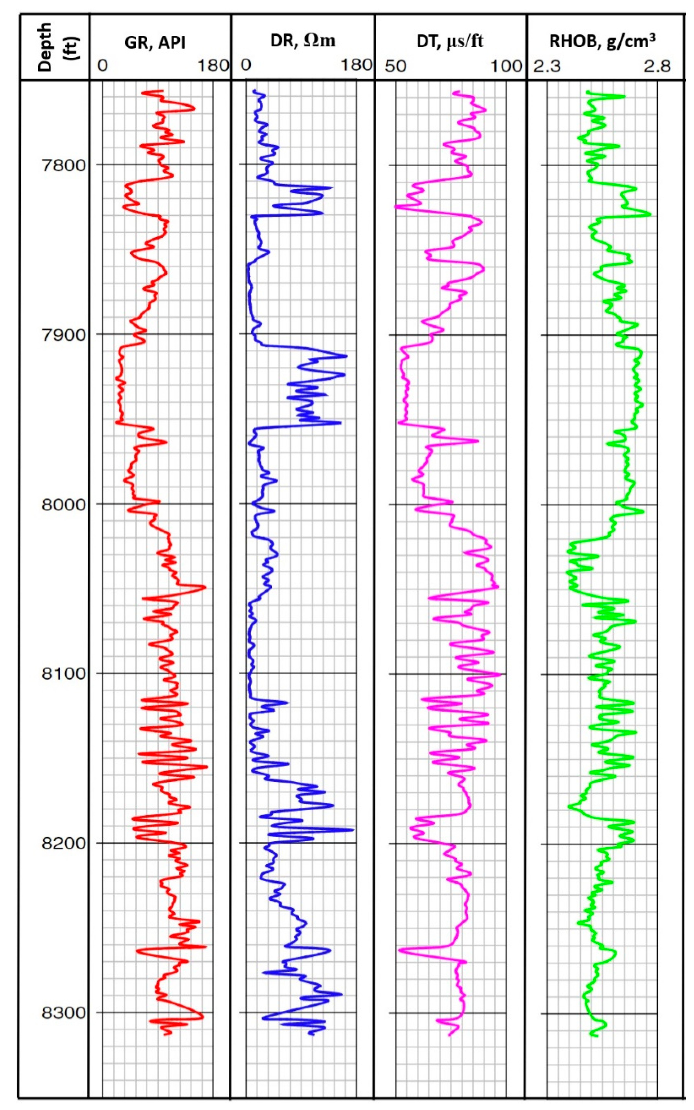
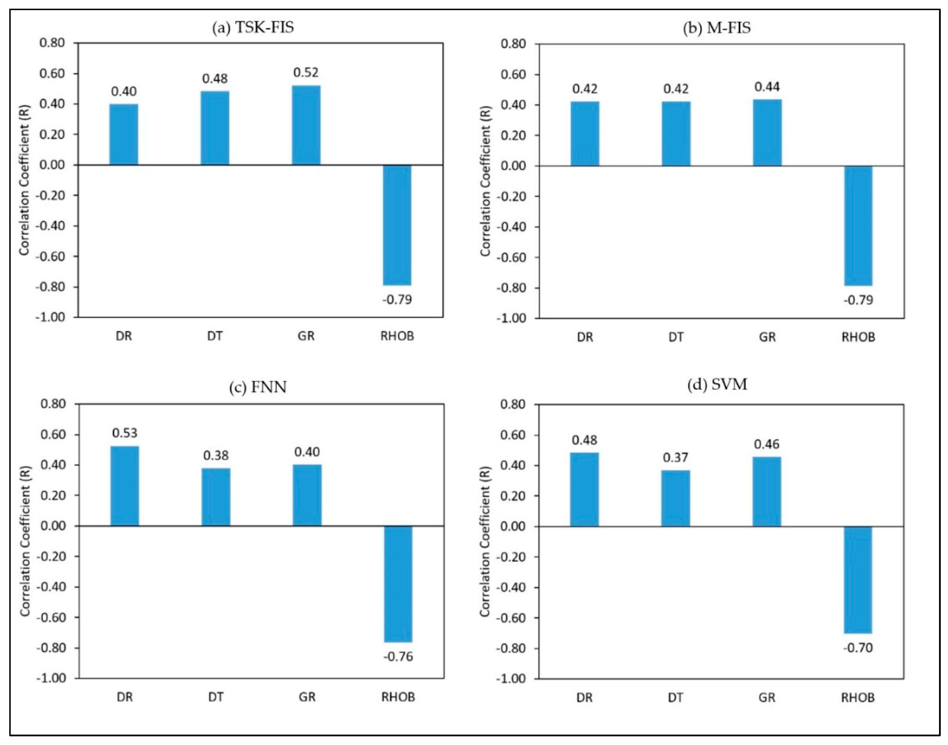
2.3. Data Description and Preprocessing

Conventional log data of DR, GR, DT, and RHOB and the corresponding actual (laboratory-measured) TOC values collected from Barnett shale formation were used to train the four AI models considered in this study. Before training, all the data was pre-processed to remove unrealistic values and outliers. After data pre-processing, 838 data points of the different well logs and their corresponding actual TOC values were found to be valid for model buildup. The use of 545, 545, 587, and 671 of the data to train TSK-FIS, M-FIS, FNN, and SVM models, respectively, were found to optimize the performance of the AI models in predicting the TOC. The number of training data was selected based on the optimization process, as discussed later in this paper.

Table 1. Statistical features of the data used to train the Takagi-Sugeno-Kang fuzzy interference system (TSK-FIS), Mamdani fuzzy interference system (M-FIS), functional neural network (FNN), and support vector machine (SVM) models.

Takagi-Sugeno-Kang Fuzzy Inference System
Data points = 545	DR, Ωm	DT, μs/ft	GR, API	RHOB, g/cm3	TOC, wt%
Minimum	4.97	50.95	23.73	2.39	0.75
Maximum	163.3	97.1	146.9	2.7	5.1
Range	158.3	46.1	123.2	0.3	4.4
Standard Deviation	40.86	9.27	24.91	0.07	1.03
Sample Variance	1670	86	621	0.0055	1.061
Mamdani Fuzzy Inference System
Data points = 545	DR, Ωm	DT, μs/ft	GR, API	RHOB, g/cm3	TOC, wt%
Minimum	4.97	53.78	28.07	2.39	0.76
Maximum	163.3	95.0	146.9	2.7	5.0
Range	158.3	41.2	118.9	0.3	4.2
Standard Deviation	38.95	8.24	22.31	0.07	0.98
Sample Variance	1517	68	498	0.0053	0.953
Functional Neural Network
Data points = 587	DR, Ωm	DT, μs/ft	GR, API	RHOB, g/cm3	TOC, wt%
Minimum	4.97	52.00	26.16	2.40	0.84
Maximum	163.6	97.1	146.9	2.7	5.1
Range	158.6	45.1	120.8	0.3	4.3
Standard Deviation	42.12	7.52	20.73	0.06	0.85
Sample Variance	1774	57	430	0.0040	0.731
Support Vector Machine
Data points = 671	DR, Ωm	DT, μs/ft	GR, API	RHOB, g/cm3	TOC, wt%
Minimum	4.97	50.95	27.37	2.39	0.76
Maximum	163.6	97.1	146.9	2.7	5.1
Range	158.6	46.1	119.6	0.3	4.4
Standard Deviation	39.81	8.20	21.63	0.07	0.96
Sample Variance	1585	67	468	0.0044	0.916

compares the different statistical features of the training data that are used to learn the four AI models developed in this study. These statistical parameters are very important for consideration when the AI models are applied to estimate the TOC using new data. In this study, before testing and validating the developed AI models, the statistical parameters of the testing and validation data were determined to ensure that these data (i.e., testing and validation data) are within the range of the training data used to develop the AI models which are summarized in Table 1.

The relative importance of the selected training well log data on the predictability of the TOC values was then studied. Figure 2 compares the relative importance between the different conventional well logs used to train the four AI models and the laboratory-measured TOC values. As indicated in Figure 2 and for the data used to train all AI models, TOC is strongly dependent on the RHOB, while it is moderately related to DR, DT, and GR.

2.4. AI Model’s Development

Four AI models namely: TSK-FIS, M-FIS, FNN, and SVM models were developed in this study to estimate the TOC using conventional well logs of DR, DT, GR, and RHOB. The four conventional well logs, used to train the AI models, were selected based on their relative importance to the core measured TOC, as discussed earlier and shown in Figure 2. However, the selection conforms to their published reported relationship with TOC. For example, DR is believed to be affected by the presence of kerogen in the source rock [41]; DT decreases with the increase in the TOC [42]; several studies have confirmed that GR could significantly enhance TOC prediction [41,43], but the relationship is controversial to others [44,45]; and RHOB decreases with the increase in the kerogen content, and hence, organic matter in the formation increases [7]. Because of the above-listed reasons, the four conventional well logs of DR, DT, GR, and RHOB are considered to develop the TOC models in this study.

All AI models were optimized for their design parameters and the training-to-testing data ratio.

Table 2. The optimum design parameters for TSK-FIS, M-FIS, FNN, and SVM models to estimate the TOC.

Takagi-Sugeno-Kang Fuzzy Inference System
Training/Testing Data Ratio	65/35
Number of Membership Functions	2
Input Membership Function	Gaussian Membership Function
Output Membership Function	Linear Function
Mamdani Fuzzy Inference System
Training/Testing Data Ratio	65/35
Cluster Radius	0.35
Number of Iterations	300
Functional Neural Network
Training/Testing Data Ratio	70/30
Training Method	Backward-Forward Selection Method
Function Type	Non-linear Function with Iteration Terms
Support Vector Machine
Training/Testing Data Ratio	80/20
Kernel	gaussian
Kerneloption	9
Lambda	1 × 10−7
Epsilon	0.5
Verbose	0.7
C	3000

summarizes the optimized design parameters of the AI models.

2.5. Evaluation Criterion

The predictability of the developed AI models, used to estimate the TOC for the training, testing, and validation data sets, was evaluated based on the absolute average percentage error “Equation (8)”, correlation coefficient “Equation (9)”, coefficient of determination “Equation (10)”, and the visual check of the actual and predicted TOC.

$$AAPE=\frac{1}{N}{\displaystyle \sum }_{i=1}^N\left(\left|\frac{{\left(R{F}_a\right)}_i-{\left(R{F}_m\right)}_i}{{\left(R{F}_a\right)}_i}\right|\times 100\right)$$

(8)

$$R=\frac{{{\displaystyle \sum }}_{i=1}^N\left[\left({\left(R{F}_a\right)}_i-\overline{R{F}_a}\right)\times \left({\left(R{F}_m\right)}_i-\overline{R{F}_m}\right)\right]}{\sqrt{{{\displaystyle \sum }}_{i=1}^N{\left[{\left(R{F}_a\right)}_i-\overline{R{F}_a}\right]}^2{{\displaystyle \sum }}_{i=1}^N{\left[{\left(R{F}_m\right)}_i-\overline{R{F}_m}\right]}^2}}$$

(9)

$$R^2={\left[\frac{{{\displaystyle \sum }}_{i=1}^N\left[\left({\left(R{F}_a\right)}_i-\overline{R{F}_a}\right) \times \left({\left(R{F}_m\right)}_i-\overline{R{F}_m}\right)\right]}{\sqrt{{{\displaystyle \sum }}_{i=1}^N{\left[{\left(R{F}_a\right)}_i-\overline{R{F}_a}\right]}^2{{\displaystyle \sum }}_{i=1}^N{\left[{\left(R{F}_m\right)}_i-\overline{R{F}_m}\right]}^2}}\right]}^2$$

(10)

where in all previous equations a and m denote the actual and estimated RF, respectively.

2.6. Application Examples to Barnett and Devonian Shale

The predictability of the four AI models considered in this study was evaluated using data of two different depositional environments. The first formation is the Mississippian Barnett shale, which was considered earlier by the United States Energy Information Administration as the main source rock of hydrocarbon in FWB [3,46]. In 2011, the proven reserve of this formation was more than 31 trillion cubic feet (TCF) with a cumulative gas production rate of 8.0 TCF. Several studies, such as Pollastro et al. [46], Romero-Sarmiento et al. [47], and Thomas [48] reported the general geologic information about Barnett shale. The second formation is the Devonian shale in WCSB, which is an organic-rich source rock in the Devonian conventional hydrocarbon system [49]. The oil and gas in place in this formation are 61.7 Billion barrels, and 443 Tcf, respectively. According to recent production data, this shale is rich in liquid [50].

3. Results and Discussion

3.1. Training the AI Models

The AI models considered in this work (TSK-FIS, M-FIS, FNN, and SVM) were trained to optimize their design parameters, the optimum design parameters of the AI models are summarized earlier in Table 2. Figure 3 compares the predictability of the four optimized AI models for the training data sets, as shown in Figure 3. The number of data used to train every AI model are different. As explained earlier, the training to testing data ratio is considered during the models optimization process, and based on this optimization, the number of training data that maximize predictability of every model is selected.

Figure 3 shows that the TSK-FIS model predicted the TOC for the training data set with the highest accuracy compared to other models, with AAPE of 7.12% and R of 0.968. M-FIS comes second with AAPE and R of 7.48% and 0.962, followed by the FNN model with AAPE of 8.05% and R of 0.936, and finally the SVM model with AAPE and R of 9.75%, and 0.933, respectively. The visual check of the plots confirms a high accuracy of the four AI models in estimating the TOC for the training data set.

Cross-plot of Figure 4 compares the measured and estimated TOC for the training data set. The narrow scattering of the points indicates the predictability of the models; TSK-FIS model is the highest with R² = 0.937, then M-FIS model with R² = 0.926, followed by FNN model with R² = 0.876, and finally SVM with the lowest R² of 0.871.

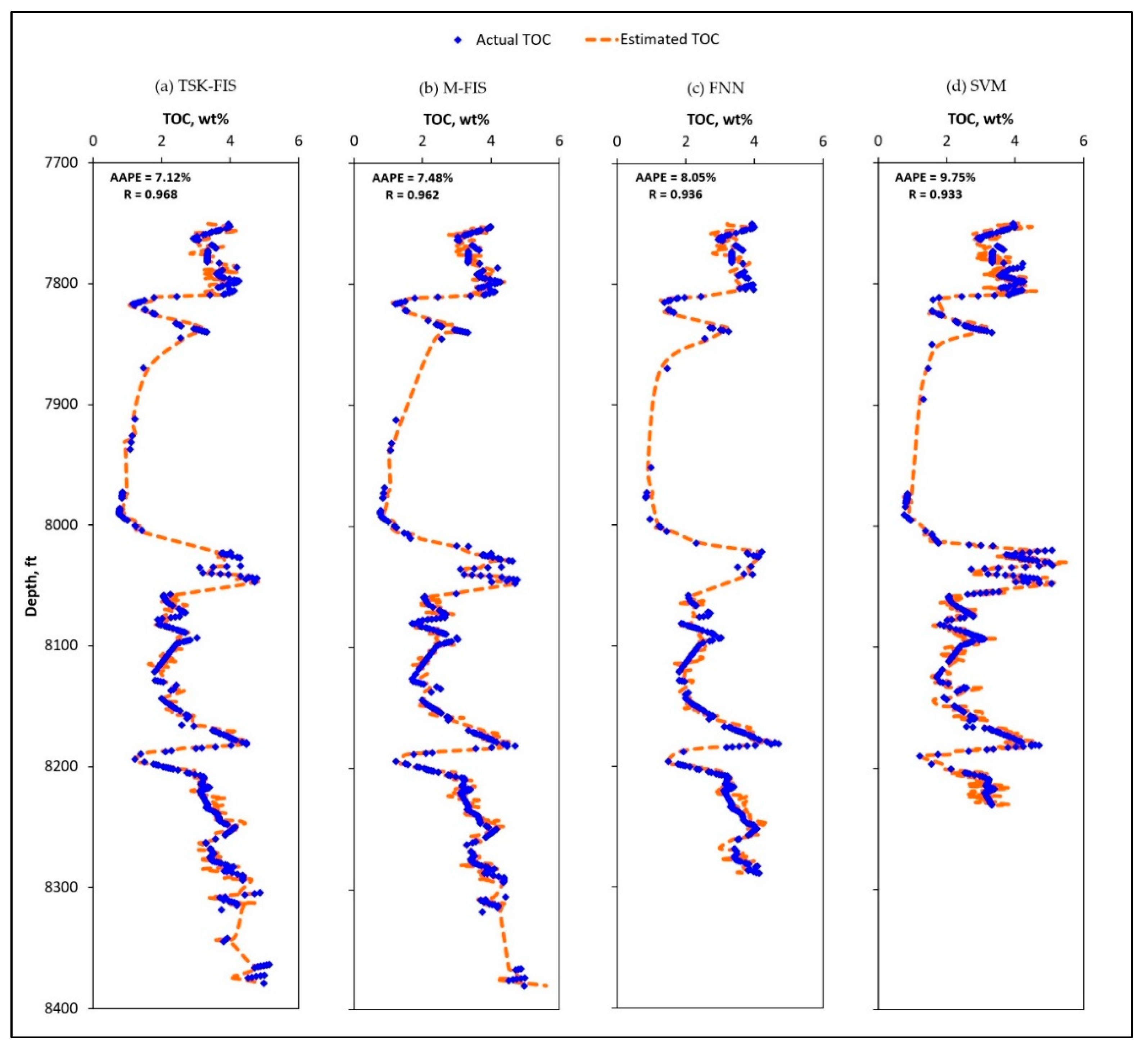
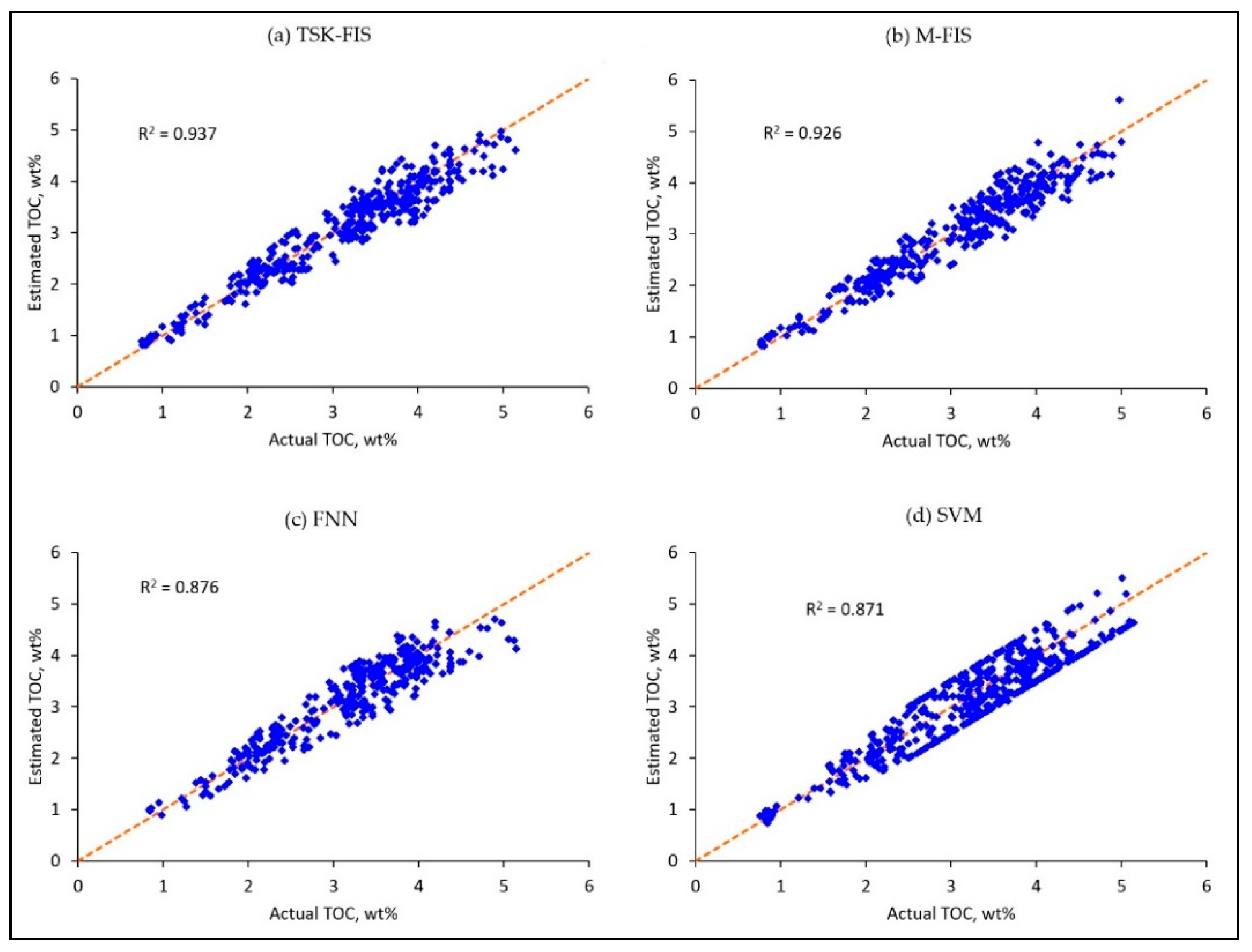
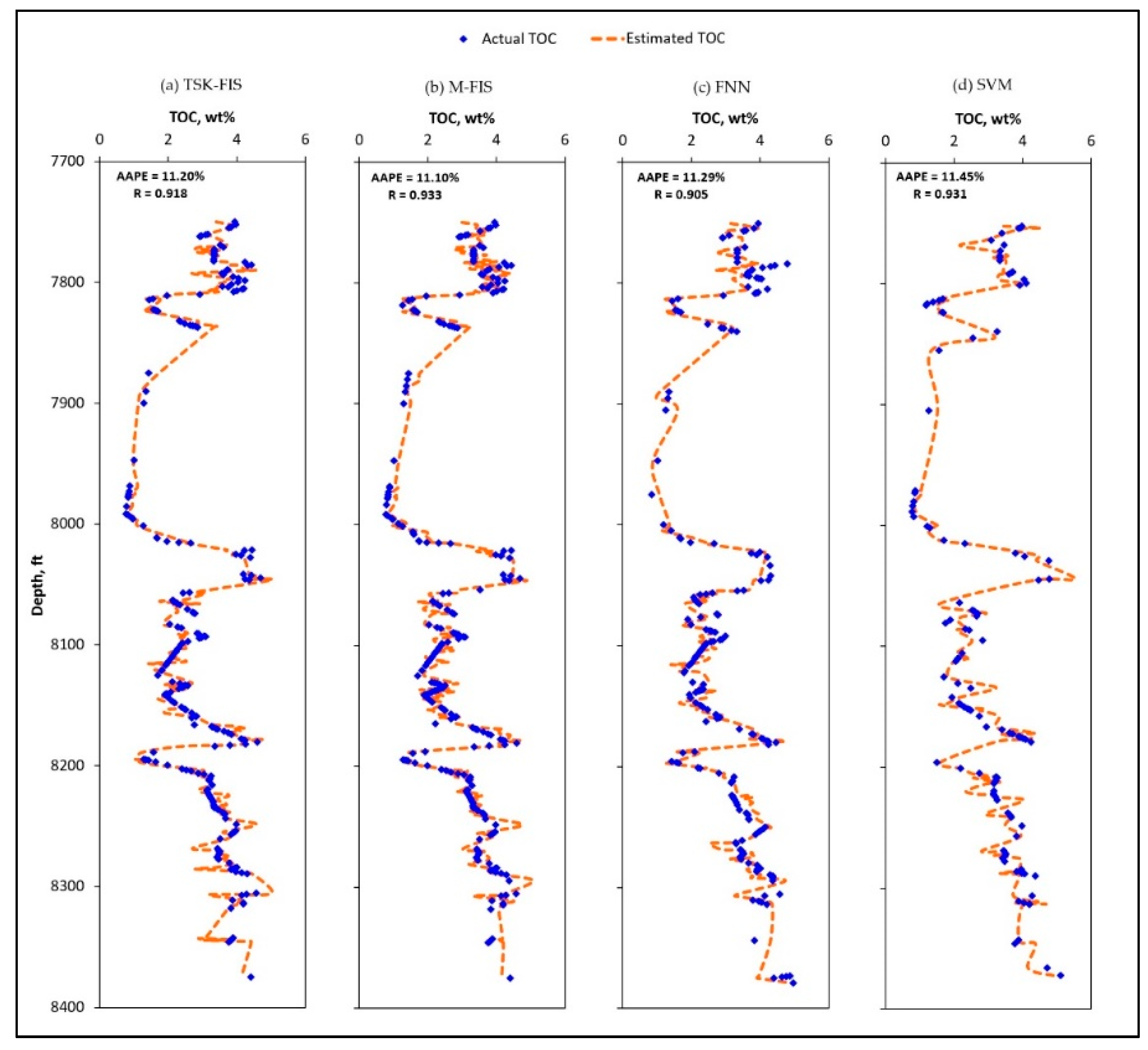
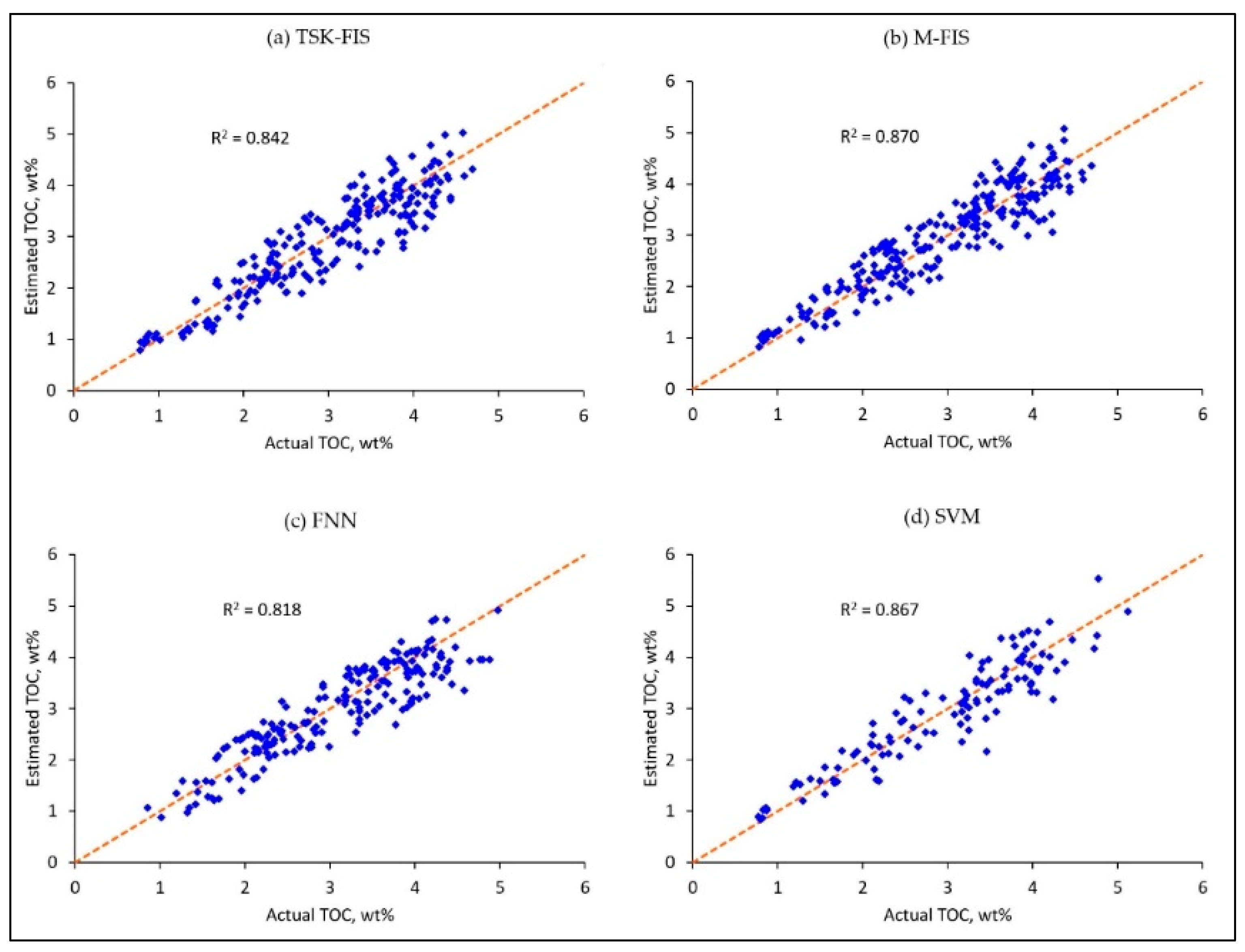
3.2. Testing the AI Models

The predictability of the four AI models, developed in this study, is then tested using data collected from the Barnett shale formation. The number of the testing data points is selected based on the optimization process as mentioned earlier.

Figure 5 compares the predictability of the AI models to evaluate the TOC for the testing data sets. Visually, the four plots indicate similar predictability for the four models, with minor differences. Considering the AAPE and R M-FIS model is the highest with 11.10% and 0.933, followed by TSK-FIS model with 11.20% and 0.918, then FNN model with 11.29% and 0.905, and finally SVM model with 11.45%, and 0.931 respectively.

The cross-plot in Figure 6 presents the correlation between measured and estimated TOC for the testing data set. The plots indicate high correlation with R² equal 0.870, 0.867, 0.842, and 0.818 for M-FIS, SVM, TSK-FIS, and FNN models, respectively.

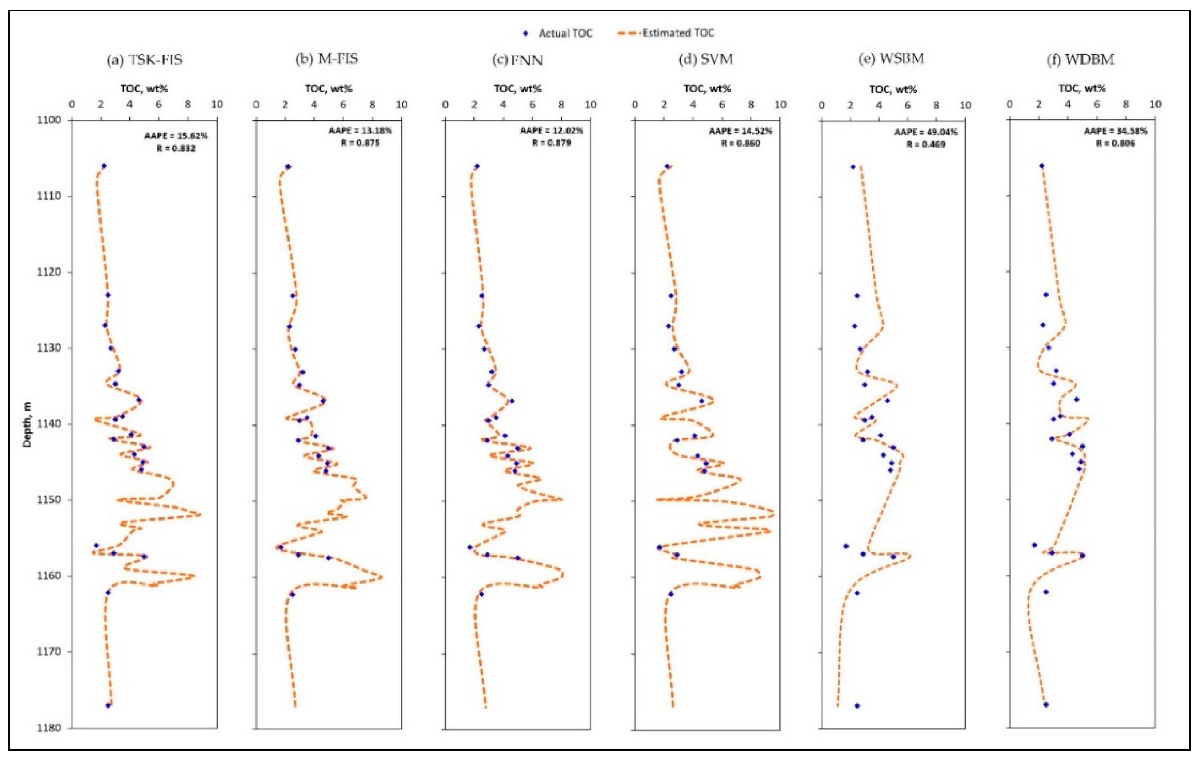
3.3. Validating the AI Models

The AI model’s validation was completed using unseen data collected from the Devonian shale formation. The total number of core derived TOC data collected from Devonian shale are 22 data points, out of these data, only 20, 19, 19, and 15 were found to fit within the range of the training data that is used to develop TSK-FIS, M-FIS, FNN, and SVM models, respectively. The range for the training data are summarized in Table 1. Based on the AAPE and R results as indicated in Figure 7, FNN model was the best model with AAPE of 12.02% and R of 0.879, followed by M-FIS model with AAPE and R of 13.18 and 0.875, then SVM with AAPE and R of 14.52% and 0.860, and finally TSK-FIS model with AAPE of 15.62% and R of 0.832 respectively. As shown in Figure 7, all AI models are highly accurate compared to Wang et al. [12] sonic- and density-based models, Wang sonic-based model (WSBM) predicted the TOC with AAPE of 34.58% and R of 0.806, while Wang density-based model (WDBM) predicted TOC with AAPE, and R of 49.04% and 0.469, respectively.

From the the results of training, testing, and validation data, considering the similarity of the results of the evaluation parameters (AAPE and R), and taking into consideration that adding or omitting a few points may change the highest-to-lowest order of the parameters, we conclude that the four models are equally adequate to estimate the TOC using only the conventional well log used in this study. Nevertheless, we recommend using the FNN model as it is the best-performed model on the validation data.

4. Conclusions

In this study, four artificial intelligence (AI) models based on Takagi-Sugeno-Kang fuzzy interference system, Mamdani fuzzy interference system, functional neural network, and support vector machine are developed to estimate the total organic carbon (TOC) using conventional well logs of deep resistivity, gamma-ray, sonic transit time, and bulk density. The models are developed and tested using data collected from Barnett shale and then validated using unseen data from Devonian shale. The optimized AI models showed a high predictability of TOC for both formations evaluated in this study. The four models are equally adequate to estimate the TOC using the well log used in this study. Nevertheless, for the validation (unseen) data considered in this study, the FNN model overperformed other models in predicting the TOC, with the lowest AAPE and the highest R, compared with other techniques. All AI models over-performed Wang models, which are recently developed to evaluate the TOC for Devonian formation.

References

1. Passey, Q.R.; Bohacs, K.; Esch, W.L.; Klimentidis, R.; Sinha, S. From oil-prone source rock to gas-producing shale reservoir-geologic and petrophysical characterization of unconventional shale gas reservoirs. In Proceedings of the International Oil and Gas Conference and Exhibition in China, Beijing, China, 8–10 June 2010. [Google Scholar]
2. Sondergeld, C.H.; Ambrose, R.J.; Rai, C.S.; Moncrieff, J. Micro-structural studies of gas shales. In Proceedings of the SPE Unconventional Gas Conference, Pittsburgh, PA, USA, 23–25 February 2010. [Google Scholar]
3. Montgomery, S.L.; Jarvie, D.M.; Bowker, K.A.; Pollastro, R.M. Mississippian Barnett Shale, Fort Worth basin, North-Central Texas: Gas-shale Play with Multi-trillion Cubic Foot Potential. Am. Assoc. Pet. Geol. Bull. 2005, 89, 155–175. [Google Scholar] [CrossRef]
4. Ross, D.J.; Bustin, R.M. Impact of mass balance calculations on adsorption capacities in microporous shale gas reservoirs. Fuel 2007, 86, 2696–2706. [Google Scholar] [CrossRef]
5. Ding, J.; Xiaozhi, C.; Xiudi, J.; Bin, W.; Jinmiao, Z. Application of AVF Inversion on Shale Gas Reservoir TOC Prediction. In Proceedings of the SEG Annual Meeting: Society of Exploration Geophysicists, New Orleans, LA, USA, 18–23 October 2015. [Google Scholar]
6. Zhang, T.; Ellis, G.S.; Ruppel, S.C.; Milliken, K.; Yang, R. Effect of organic-matter type and thermal maturity on methane adsorption in shale-gas systems. Org. Geochem. 2012, 47, 120–131. [Google Scholar] [CrossRef]
7. Schmoker, J.W. Determination of Organic Content of Appalachian Devonian Shales from Formation-Density Logs. Am. Assoc. Pet. Geol. Bull. 1979, 63, 1504–1509. [Google Scholar] [CrossRef]
8. Schmoker, J.W. Organic content of Devonian shale in Western Appalachian Basin. Am. Assoc. Pet. Geol. Bull. 1980, 64, 2156–2165. [Google Scholar]
9. Passey, Q.R.; Creaney, S.; Kulla, J.B.; Moretti, F.J.; Stroud, J.D. A practical model for organic richness from porosity and resistivity logs. Am. Assoc. Pet. Geol. Bull. 1990, 74, 1777–1794. [Google Scholar]
10. Charsky, A.; Herron, S. Accurate, direct Total Organic Carbon (TOC) log from a new advanced geochemical spectroscopy tool: Comparison with conventional approaches for TOC estimation. In Proceedings of the AAPG Annual Convention and Exhibition, Pittsburg, PA, USA, 19–22 May 2013. [Google Scholar]
11. Wang, J.; Gu, D.; Guo, W.; Zhang, H.; Yang, D. Determination of Total Organic Carbon Content in Shale Formations With Regression Analysis. J. Energy Resour. Technol. 2019, 141, 012907. [Google Scholar] [CrossRef]
12. Wang, P.; Chen, Z.; Pang, X.; Hu, K.; Sun, M.; Chen, X. Revised models for determining TOC in shale play: Example from Devonian Duvernay Shale, Western Canada Sedimentary Basin. Mar. Pet. Geol. 2016, 70, 304–319. [Google Scholar] [CrossRef]
13. Zhu, L.; Zhang, C.; Zhang, Z.; Zhou, X.; Liu, W. An improved method for evaluating the TOC content of a shale formation using the dual-difference ΔlogR method. Mar. Pet. Geol. 2019, 102, 800–816. [Google Scholar] [CrossRef]
14. Wang, H.; Wu, W.; Chen, T.; Dong, X.; Wang, G. An improved neural network for TOC, S1 and S2 estimation based on conventional well logs. J. Pet. Sci. Eng. 2019, 176, 664–678. [Google Scholar] [CrossRef]
15. Zhu, L.; Zhang, C.; Zhang, C.; Zhang, Z.; Nie, X.; Zhou, X.; Liu, W.; Wang, X. Forming a new small sample deep learning model to predict total organic carbon content by combining unsupervised learning with semisupervised learning. Appl. Soft Comput. 2019, 83, 105596. [Google Scholar] [CrossRef]
16. Zhu, L.; Zhang, C.; Zhang, C.; Zhou, X.; Wang, J.; Wang, X. Application of Multiboost-KELM algorithm to alleviate the collinearity of log curves for evaluating the abundance of organic matter in marine mud shale reservoirs: A case study in Sichuan Basin, China. Acta Geophys. 2018, 66, 983. [Google Scholar] [CrossRef]
17. Crain, E.R. Petrophysical Handbook. 2000. Available online: https://spec2000.net/11-vshtoc.htm (accessed on 20 July 2019).
18. Mahmoud, A.A.A.; Elkatatny, S.; Mahmoud, M.; Abouelresh, M.; Abdulraheem, A.; Ali, A. Determination of the total organic carbon (TOC) based on conventional well logs using artificial neural network. Int. J. Coal Geol. 2017, 179, 72–80. [Google Scholar] [CrossRef]
19. Mahmoud, A.A.; Elkatatny, S.; Abdulraheem, A.; Mahmoud, M.; Ibrahim, M.O.; Ali, A. New Technique to Determine the Total Organic Carbon Based on Well Logs Using Artificial Neural Network (White Box). In Proceedings of the SPE Kingdom Saudi Arabia Annual Technical Symposium and Exhibition, Dammam, Saudi Arab, 24–27 April 2017. [Google Scholar]
20. Elkatatny, S. A Self-Adaptive Artificial Neural Network Technique to Predict Total Organic Carbon (TOC) Based on Well Logs. Arab. J. Sci. Eng. 2018, 44, 6127–6137. [Google Scholar] [CrossRef]
21. Mohaghegh, S.; Arefi, R.; Ameri, S.; Hefner, M.H. A Methodological Approach for Reservoir Heterogeneity Characterization Using Artificial Neural Networks. In Proceedings of the SPE Annual Technical Conference and Exhibition, New Orleans, LA, USA, 25–28 September 1994. [Google Scholar]
22. Barman, I.; Ouenes, A.; Wang, M. Fractured Reservoir Characterization Using Streamline-Based Inverse Modeling and Artificial Intelligence Tools. In Proceedings of the SPE Annual Technical Conference and Exhibition, Dallas, TX, USA, 1–4 October 2000. [Google Scholar]
23. Elkatatny, S.A.; Mahmoud, M.A. Development of a New Correlation for Bubble Point Pressure in Oil Reservoirs Using Artificial Intelligent Technique. Arab. J. Sci. Eng. 2018, 43, 2491–2500. [Google Scholar] [CrossRef]
24. Elkatatny, S.M. Real Time Prediction of Rheological Parameters of KCl Water-Based Drilling Fluid Using Artificial Neural Networks. Arab. J. Sci. Eng. 2017, 42, 1655–1665. [Google Scholar] [CrossRef]
25. Abdelgawad, K.; Elkatatny, S.; Moussa, T.; Mahmoud, M.; Patil, S. Real Time Determination of Rheological Properties of Spud Drilling Fluids Using a Hybrid Artificial Intelligence Technique. J. Energy Resour. Technol. 2018. [Google Scholar] [CrossRef]
26. Al-AbdulJabbar, A.; Elkatatny, S.M.; Mahmoud, M.; Abdelgawad, K.; Abdulaziz, A. A Robust Rate of Penetration Model for Carbonate Formation. J. Energy Resour. Technol. 2019, 141, 042903. [Google Scholar] [CrossRef]
27. Elkatatny, S. Application of Artificial Intelligence Techniques to Estimate the Static Poisson’s Ratio Based on Wireline Log Data. J. Energy Resour. Technol. 2018, 140, 072905. [Google Scholar] [CrossRef]
28. Mahmoud, A.A.; Elkatatny, S.; Ali, A.; Moussa, T. Estimation of Static Young’s Modulus for Sandstone Formation Using Artificial Neural Networks. Energies 2019, 12, 2125. [Google Scholar] [CrossRef]
29. Ahmed, A.S.; Mahmoud, A.A.; Elkatatny, S. Fracture Pressure Prediction Using Radial Basis Function. In Proceedings of the AADE National Technical Conference and Exhibition, Denver, CO, USA, 9–10 April 2019. [Google Scholar]
30. Ahmed, A.S.; Mahmoud, A.A.; Elkatatny, S.; Mahmoud, M.; Abdulraheem, A. Prediction of Pore and Fracture Pressures Using Support Vector Machine. In Proceedings of the 2019 International Petroleum Technology Conference, Beijing, China, 26–28 March 2019. [Google Scholar]
31. Al-Shehri, D.A. Oil and Gas Wells: Enhanced Wellbore Casing Integrity Management through Corrosion Rate Prediction Using an Augmented Intelligent Approach. Sustainability 2019, 11, 818. [Google Scholar] [CrossRef]
32. Salehi, S.; Hareland, G.; Dehkordi, K.K.; Ganji, M.; Abdollahi, M. Casing collapse risk assessment and depth prediction with a neural network system approach. J. Pet. Sci. Eng. 2009, 69, 156–162. [Google Scholar] [CrossRef]
33. Mahmoud, A.A.; Elkatatny, S.; Abdulraheem, A.; Mahmoud, M. Application of Artificial Intelligence Techniques in Estimating Oil Recovery Factor for Water Drive Sandy Reservoirs. In Proceedings of the SPE Kuwait Oil & Gas Show and Conference, Kuwait City, Kuwait, 15–18 October 2017. [Google Scholar]
34. Mahmoud, A.A.; Elkatatny, S.; Chen, W.; Abdulraheem, A. Estimation of Oil Recovery Factor for Water Drive Sandy Reservoirs through Applications of Artificial Intelligence. Energies 2019, 12, 3671. [Google Scholar] [CrossRef]
35. Wang, Y.; Salehi, S. Application of real-time field data to optimize drilling hydraulics using neural network approach. J. Energy Resour. Technol. 2015, 137. [Google Scholar] [CrossRef]
36. Amato, F.; Moscato, V.; Picariello, A.; Sperl, G. Recommendation in Social Media Networks. In Proceedings of the 2017 IEEE Third International Conference on Multimedia Big Data (BigMM), Laguna Hills, CA, USA, 19–21 April 2017. [Google Scholar]
37. Su, X.; Sperli, G.; Moscato, V.; Picariello, A.; Esposito, C.; Choi, C. An Edge Intelligence Empowered Recommender System Enabling Cultural Heritage Applications. IEEE Trans. Ind. Inform. 2019, 15, 4266–4275. [Google Scholar] [CrossRef]
38. Carvajal-Ortiz, H.; Gentzis, T. Critical considerations when assessing hydrocarbon plays using Rock-Eval pyrolysis and organic petrology data: Data quality revisited. Int. J. Coal Geol. 2015, 152, 113–122. [Google Scholar] [CrossRef]
39. Chen, Z.; Jiang, C.; Lavoie, D.; Reyes, J. Model-assisted Rock-Eval data interpretation for source rock evaluation: Examples from producing and potential shale gas resource plays. Int. J. Coal Geol. 2016, 165, 290–302. [Google Scholar] [CrossRef]
40. Hazra, B.; Dutta, S.; Kumar, S. TOC calculation of organic matter rich sediments using Rock-Eval pyrolysis: Critical consideration and insights. Int. J. Coal Geol. 2016, 169, 106–115. [Google Scholar] [CrossRef]
41. Heslop, K.A. Generalized Method for the Estimation of TOC from GR and Rt. In Proceedings of the AAPG Annual Convention and Exhibition, New Orleans, LA, USA, 11–14 April 2010. [Google Scholar]
42. Liu, Y.; Chen, Z.; Hu, K.; Liu, C. Quantifying Total Organic Carbon (TOC) from Well Logs Using Support Vector Regression. GeoConvention 2013, Calgary, Canada. Available online: https://www.geoconvention.com/archives/2013/281_GC2013_Quantifying_Total_Organic_Carbon.pdf (accessed on 15 July 2019).
43. Zhao, T.; Verma, S.; Devegowda, D. TOC estimation in the Barnett Shale from Triple Combo logs Using Support Vector Machine. In Proceedings of the 85th Annual International Meeting of the SEG, New Orleans, LA, USA, 18–23 October 2015; pp. 791–795. [Google Scholar]
44. Gonzalez, J.; Lewis, R.; Hemingway, J.; Grau, J.; Rylander, E.; Pirie, I. Determination of Formation Organic Carbon Content Using a New Neutron-Induced Gamma Ray Spectroscopy Service that Directly Measures Carbon. In Proceedings of the SPWLA 54th Annual Logging Symposium, New Orleans, LA, USA, 22–26 June 2013. [Google Scholar]
45. Luning, S.; Kolonic, S. Uranium Spectral Gamma-Ray Response as a Proxy for Organic Richness in Black Shales: Applicability and Limitations. J. Pet. Geol. 2003, 26, 153–174. [Google Scholar] [CrossRef]
46. Pollastro, R.M.; Jarvie, D.M.; Hill, R.J.; Adams, C. Geologic Framework of the Mississippian Barnett Shale, Barnett-Paleozoic Total Petroleum System, Bend Arch-Fort Worth Basin, Texas. Am. Assoc. Pet. Geol. Bull. 2007, 91, 405–436. [Google Scholar] [CrossRef]
47. Romero-Sarmiento, M.F.; Ducros, M.; Carpentier, B.; Lorant, F.; Cacas, M.C.; Pegaz-Fiornet, S.; Wolf, S.; Rohais, S.; Moretti, I. Quantitative Evaluation of TOC, Organic Porosity and Gas Retention Distribution in a Gas Shale Play Using Petroleum System Modeling: Application to the Mississippian Barnett Shale. Mar. Pet. Geol. 2013, 45, 315–330. [Google Scholar] [CrossRef]
48. Thomas, J.D. Integrating Synsedimentary Tectonics with Sequence Stratigraphy to Understand the Development of the Fort Worth Basin. In Proceedings of the AAPG Southwest Section Meeting, Ruidoso, NM, USA, 6–8 June 2002. [Google Scholar]
49. Creaney, S.; Allan, J.; Cole, K.S.; Fowler, M.G.; Brooks, P.W.; Osadetz, K.G.; Riediger, C.L. Petroleum Generation and Migration in the Western Canada Sedimentary Basin. In Geological Atlas of the Western Canada Sedimentary Basin; Canadian Society of Petroleum Geologists: Calgary, AB, Canada, 1994; pp. 455–468. [Google Scholar]
50. Rokosh, C.D.; Lyster, S.; Anderson, S.D.A.; Beaton, A.P.; Berhane, H.; Brazzoni, T.; Chen, D.; Cheng, Y.; Mack, T.; Pana, C.; et al. Summary of Alberta’s Shale-and Siltstone-Hosted Hydrocarbon Resource Potential; Energy Resources Conservation Board: Edmonton, AB, Canada, 2012. [Google Scholar]
Figure 1. Well log data collected from Barnett shale formation to develop the AI models.
Sustainability 11 05643 g001
Figure 2. The relative importance of the data used to train (a) Takagi-Sugeno-Kang fuzzy interference system (TSK-FIS), (b) Mamdani fuzzy interference system (M-FIS), (c) functional neural network (FNN), and (d) support vector machine (SVM) models.
Sustainability 11 05643 g002
Figure 3. Comparison of measured and estimated TOC using (a) TSK-FIS, (b) M-FIS, (c) FNN, and (d) SVM for the training data sets.
Sustainability 11 05643 g003
Figure 4. Cross-plot of the measured and estimated TOC using (a) TSK-FIS, (b) M-FIS, (c) FNN, and (d) SVM for the training data set.
Sustainability 11 05643 g004
Figure 5. Comparison of measured and estimated TOC using (a) TSK-FIS, (b) M-FIS, (c) FNN, and (d) SVM for the testing data sets.
Sustainability 11 05643 g005
Figure 6. Cross-plot of the measured and estimated TOC using (a) TSK-FIS, (b) M-FIS, (c) FNN, and (d) SVM for the testing data sets.
Sustainability 11 05643 g006
Figure 7. Comparison of measured and estimated TOC using (a) TSK-FIS, (b) M-FIS, (c) FNN, (d) SVM, (e) WSBM, and (f) WDBM for the validation data sets.
Sustainability 11 05643 g007