Article

The Extent of Infrastructure Causing Fragmentation in the Hydrocarbon Basin in the Arid and Semi-Arid Zones of Patagonia (Argentina)

1
Departamento de Biología y Ambiente, Universidad Nacional de la Patagonia San Juan Bosco, Chubut 9000, Argentina
2
INIBIOMA, CONICET, Universidad Nacional del Comahue, Río Negro 8400, Argentina
3
CNR-IMAA C, da S. Loya Tito zona Industriale, 85050 Potenza, Italy
*
Author to whom correspondence should be addressed.
Sustainability 2019, 11(21), 5956; https://0-doi-org.brum.beds.ac.uk/10.3390/su11215956
Submission received: 20 June 2019 / Revised: 20 August 2019 / Accepted: 6 September 2019 / Published: 25 October 2019
(This article belongs to the Special Issue Remote Sensing for Archaeology and Cultural Landscapes)

Abstract

:
Fragmentation is a disruption in the connectivity of landscapes. The aims of this paper are (i) to quantitatively assess the fragmentation rates in three landscape units located in a hydrocarbon basin, and (ii) to model their behavior between 2001 and 2013 using landscape metrics at different scales of resolution. The following metrics were selected using principal component analysis (PCA): The Clumpiness Index (CLUMPY), patch density (PD), perimeter-area fractal dimension (PAFRAC) and effective mesh size (MESH). Results from our investigations pointed out that hydrocarbon activity increased the fragmentation at the sites. In particular, the CLUMPY index increased in all three landscape units, the average of PD decreased from 60 to 14 patches per 100 hectares, whereas the mean of MESH was quite constant, however, due to oil production, it decreased mainly in the coastal valleys. Finally, the PAFRAC also decreased at sites with oil production, being more evident in the plateau and coastal canyons. As a whole, outputs from our analyses clearly pointed out that the monitoring of landscape fragmentation trends in arid and semi-arid zones can be successfully achieved using metrics derived from satellite spectral information.

1. Introduction

Oil resources are geographically unevenly distributed throughout the world. The concentration of reserves does not coincide with the main consumption areas, being that, in general, the concentration of reserves is in developing countries, whereas, most of the industrialized countries are importers of oil. The main oil consumers are as follows: The United States of America, Japan and Germany, while the main producers are Saudi Arabia, the United States of America and the countries of the North Sea (such as Norway and the United Kingdom). In terms of the ranking of producing countries, Argentina is positioned in 25th place [1]. In Argentina, the oil exploitation started in 1907 in the San Jorge Gulf basin (Chubut and Santa Cruz provinces). This basin has a total area estimated at around 200,000 km2 and currently produces around 37,000 m3 of oil per day, obtained from more than 6000 oil wells (9000 are inactive) [2].
The oil industry has significant economic importance in both producing and consumer countries, being that it is a crucial element of national and international economic policies. According to the cycles that characterize this economic activity, the oil industry had a production crisis that declined during the years of 2009 to 2014. Future exploration projects will focus on obtaining oil through non-conventional techniques in mature fields where the application of assisted recovery techniques is mandatory [3]. These techniques are carried out by injecting water or natural gas or steam, polymers and bacteria into injection wells, in order to extract oil [4].
This paper focuses on the estimation of the impact of the oil industry in the landscape of San Jorge Gulf. Therein, the oil industry is one of the main anthropic disturbances that alters landscape patterns and generates new patches and corridors extensively used as sheep farming. In the proposed approach, the first step (prospecting) is to identify oil reserves using remote sensing with seismic and geological information. Companies build extraction facilities, roads, and pipelines as logistic infrastructures necessary for exploitation activities. The techniques of oil extraction require the use of explosives to rupt the rock [5] and extract hydrocarbon, that is later transported to the refineries and, finally, to the places where it is sold. Potential environmental impacts can occur along the diverse steps of exploration, exploitation and transportation, including the following, for example; (i) potential soil contamination due to losses caused by ruptures of pipelines, (ii) soil salinization produced by purge waters, (iii) loss of top-soil, (iv) soil compaction, (v) modification of topography, (vi) alteration of water dynamics in prairies (known locally as “mallines”) and coastal valleys for the construction of roads and extraction facilities [6].
Landscape ecology provides tools for the analysis of the landscape pattern, i.e., discrete characteristics, composition and spatial layout. For example, in North Dakota, Christie et al. [7] focused on the inverse relationship between the index of pronghorn (Antilocapra americana) abundance and oil well density; in Texas (USA) Pierre et al. [8] quantified direct landscape alteration and fragmentation, along with the effects on biodiversity resulting from oil/gas infrastructure and wind energy development. Birdsall et al. [9] focused on the propagation of exotic species and the oil industry, and Milt et al. [10] investigated multiple environmental impacts associated with shale gas infrastructure development.
This paper is focused on the study of causes and consequences of land use changes that generate processes of landscape fragmentation, loss of connectivity and interruptions in ecological flows [11]. Fragmentation is defined as a disruption in landscape connectivity [12], that facilitates (to a greater or lesser extent) the ecological flows of matter and energy across the territory [13]. To quantify functional connectivity, it is necessary to consider the impacts and constraints imposed by the increasing rate of changes in the landscape and the environment. These changes are mainly driven by socio-economic factors that in turn put pressure on natural landscapes [14]. Structural connectivity is a measure of the size, shape and configuration of the habitats in a landscape’s mosaic [15] and it is one of the best responses for mitigating the negative effects of habitat fragmentation [16]. The consequences of habitat fragmentation and the associated loss of connectivity have been studied in the light of the theory of island biogeography [17] and the patch-matrix-corridor model [11]. The latter has been used in habitats modified by agriculture [18,19,20,21], in wooded [22,23], arid [24] and semi-arid areas [25]. Nevertheless, studies of landscape fragmentation produced by oil activity in arid and semi-arid zones are still today quite scarce, especially in vulnerable arid and semi-arid zones as in the case of the Chubut and Santa Cruz provinces of Argentina, where a severe desertification process is currently ongoing.
One of the most important factors in conservation and restoration plans is the knowledge and quantification of how human activities impact on landscape structure and dynamics, which may be highly variable in time and space [26]. Numerous landscape metrics have been developed from thematic maps generated from satellite information to improve the understanding of the spatial arrangement between different classes of land use land cover, especially for assessing fragmentation rates [27]. These metrics provide valuable information for monitoring ecological processes and their evolutions mainly because they simultaneously measure landscape structure and configuration. However, inadequate selections of metrics can lead to conceptual errors [28], since there are several alternatives for representing landscapes; for example, mean size and patch density provide redundant information. To overcome this drawback, statistical analyses, such as clusters, and multivariate principal component analysis (PCA) are commonly used to effectively select representative metrics, reducing the number of indicators and avoiding redundancy [28,29,30]. In particular, PCA is a technique that reduces variable redundancy and extracts uncorrelated information represented by a new set of orthogonal (uncorrelated) variables [29,30,31,32].
In the hydrocarbon basin under investigation in this paper, the main anthropogenic disturbances that alter landscape patterns and generate new patches and corridors are mainly sheep farming and the petroleum industry. In particular, the latter generates roads, extraction facilities, machinery service areas, and pipelines built during the different stages of exploration, exploitation and transportation, thus producing specific disturbances such as the removal of vegetation cover and soil compaction [33]. In extra-Andean Patagonia, sheep were introduced at the beginning of the 20th century through a system of farms with sizes ranging from 10,000 to 50,000 ha [34,35]. Sheep grazing is considered one of the largest consumers of natural vegetation at a global level [36,37] since it generates changes in vegetation communities [38] and affects soil structure and resources.
In 2003, Latin America entered the Commodities Consensus [39], that underlines the consolidation of a new economic, political and ideological order, sustained by the boom in international prices of raw materials and consumer goods demanded by wealthier nations and emerging powers, which generates undoubted comparative advantages in economic growth, but at the same time, produces new asymmetries and deep inequalities in Latin American societies. Oil exploitation has been characterized by cyclical behaviors with ups and downs, as for example, in the boom of the last decade and the crisis currently ongoing today. In 2015, the price of an oil barrel fell by 41% in relation to the previous year, and according to the International Energy Agency, the price remained low throughout the whole 2016 year.
The aim of this study is to quantitatively evaluate landscape fragmentation in the hydrocarbon basin located in the arid and semi-arid zones of Patagonia (Argentina) over a period of 12 years. To this aim, the smallest package of metrics that best explain the fragmentation process in the study area has been herein selected, analyzed and discussed. In particular, we sought to quantify the fragmentation rates in three landscape units and to explain their behavior between 2001 and 2013, using landscape metrics at different scales of resolution. This enabled us to quantify the effects of fragmentation and support a mitigation strategy to reduce the environmental impacts produced by the oil industry.

2. Materials and Methods

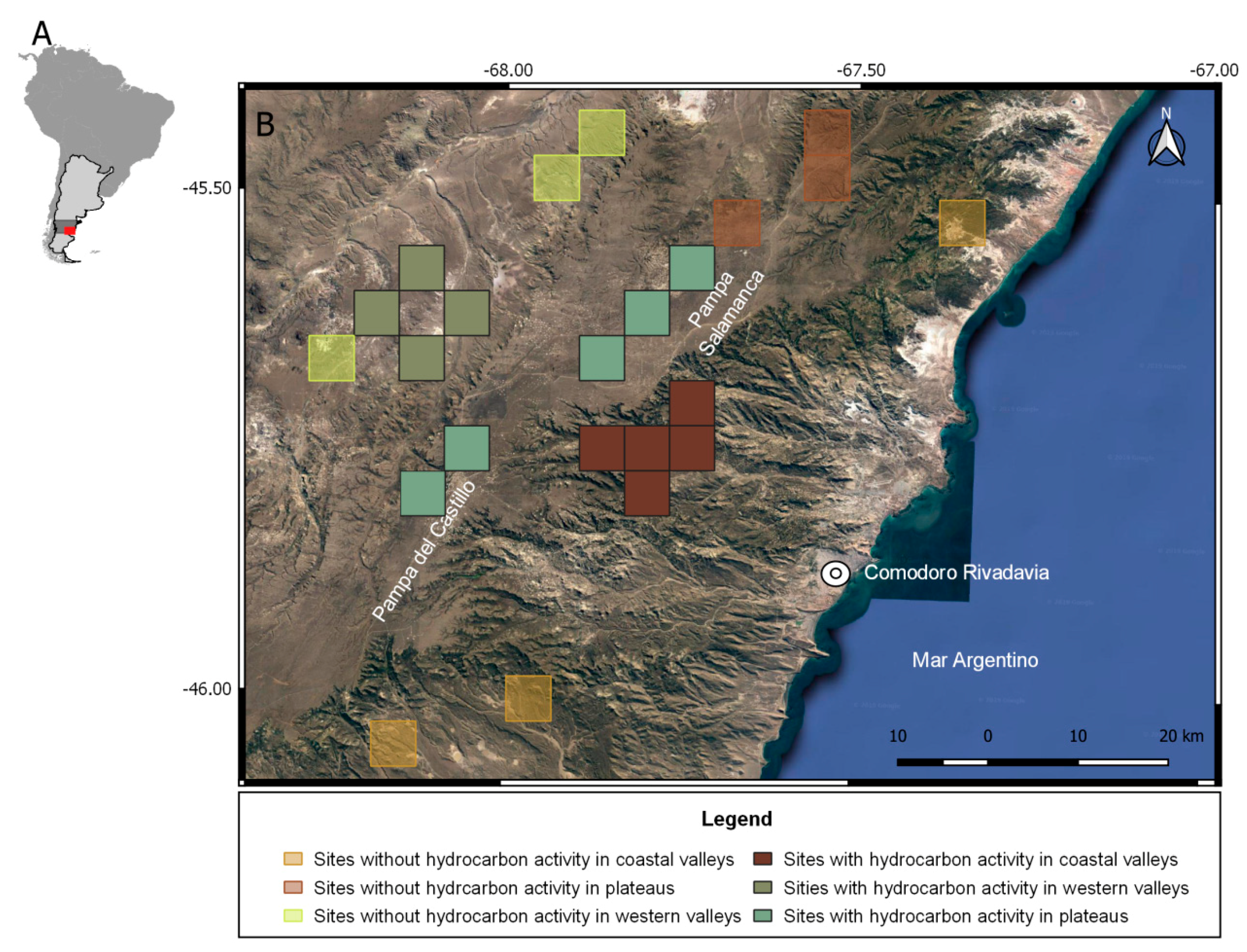
2.1. The Study Was Performed in the Hydrocarbon Basin Located in the Chubut and Santa Cruz Provinces
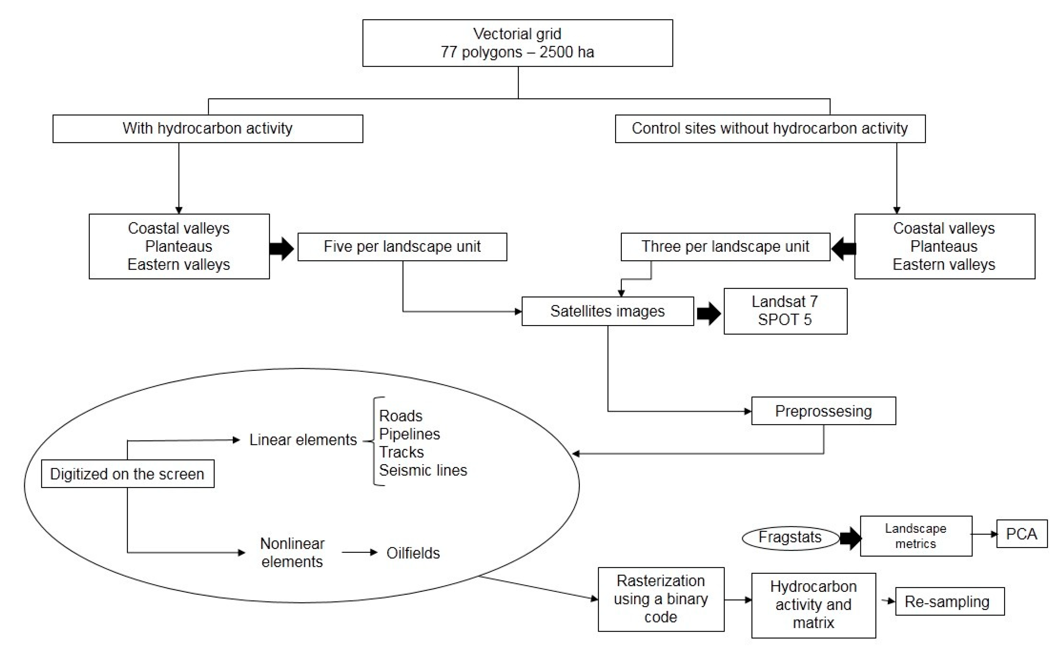
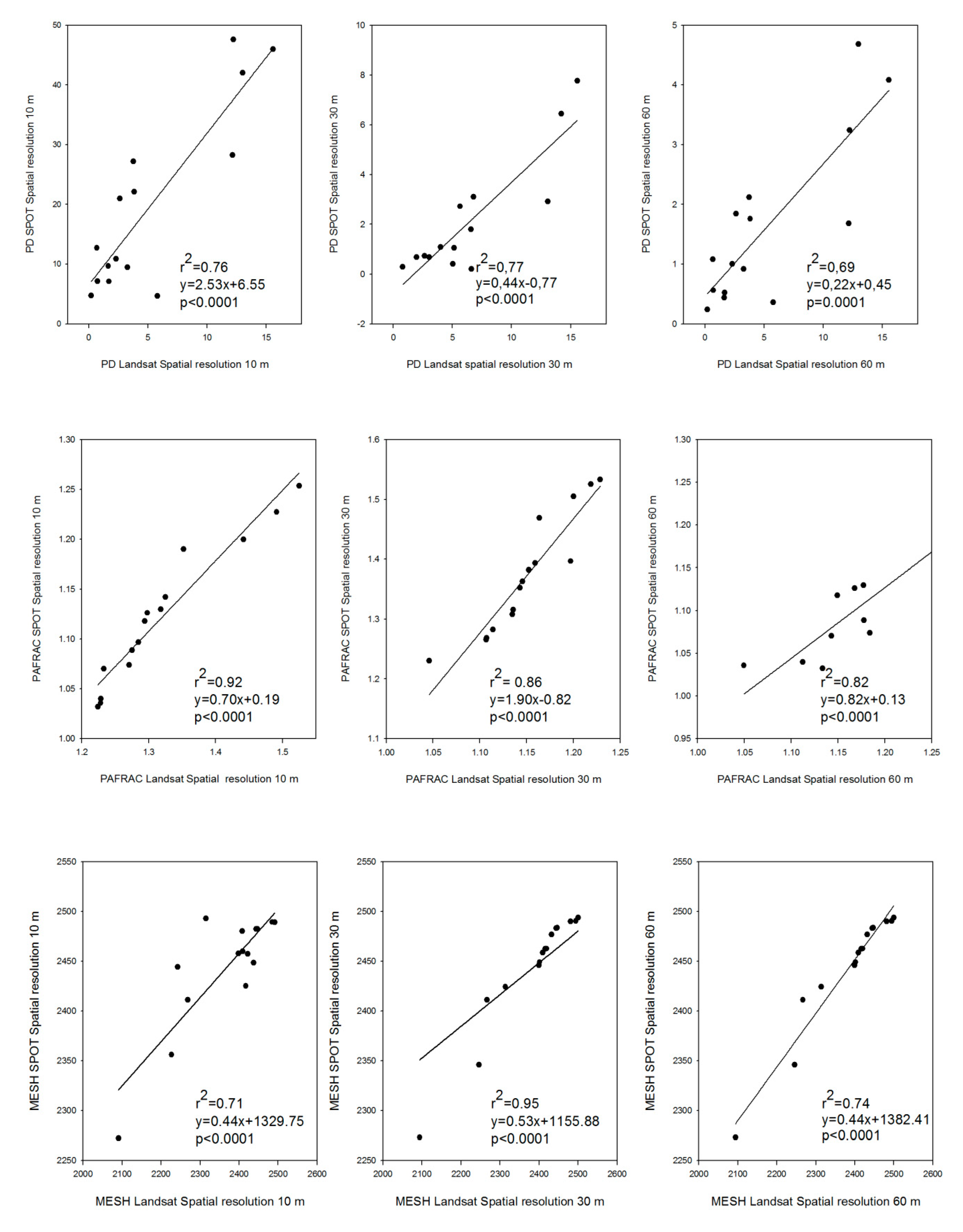
The hydrocarbon basin of San Jorge Gulf covers an area of approximately 170,000 km2, and is located in Patagonia, Argentina (Figure 1). The most important city in the region is Comodoro Rivadavia with a total of 186,583 habitants [40]. This region is divided into three landscape units that from east to west are as follows: The western valleys, the plateaus and the coastal valleys. The western valleys have an area of 532 km2 and are located in the phytogeographic region of the Central District, Subdistrito Chubutense [41], which is the most widespread unit in Central Patagonia. The plateaus have an area of 628 km2, among them, the main ones are as follows: Pampa del Castillo and Pampa Salamanca, with an average height of approximately 750 m, constituting one of the most important topographic features of the zone. It has a southwest–northeast orientation, from where many canyons originate, sloping towards the Atlantic. The coastal valleys have a surface area of approximately 300 km2, the boundary is the supra-tidal line on San Jorge Gulf (Mar Argentino), the northern and western boundaries are at the maximum level of the plateaus of Castillo and Salamanca; the southern limit is at latitude 45°48′ S. In this region the climate is semi-arid and cold. The mean annual temperature is 13 °C and precipitation is concentrated during the coldest months of the year (June and July). The average precipitation is 247.50 mm (1981–2010) [42].

2.2. Methods

The analysis herein performed was based on the following steps: (i) Selection of sampling sites with and without hydrocarbon activity in the landscape units (Figure 2), (ii) digitization of landscape elements, (iii) calculation of metrics, (iv) running PCA and selection of the most representative landscape metrics; (v) re-sampling of the satellite images; and (vi) analysis of the obtained results. A summary of these methods is shown in Figure 3.
A grid was drawn in vector format to randomly select five sampling sites for each landscape unit with hydrocarbon activity and (three) control sites without hydrocarbon activity.
High resolution multispectral SPOT 5 satellite images (19 February 2013) were used along with Landsat 7 Enhanced Thematic Mapper Plus (ETM +) of medium spatial resolution (19 December 2001). The data pre-processing consisted in rectification, co-registration and resampling of the different spatial resolutions (10, 30, 60 m) made using the closest neighbor (with an error less than 0.5) [43]. Both of the two images were rectified to the plane coordinate system POSGAR 1994.
A mesh of 77 polygons were placed on the satellite images in a vector format with a resolution of 2500 ha. Five random sites were selected in each of the landscape units where both the linear (roads, tracks, pipelines and seismic lines) and nonlinear elements (oilfields) were digitized. Then the transformation of the vector files to raster images was carried out. The rasterization of the initial maps was generated using a binary code: Anthropogenic activity (linear + nonlinear elements) and the matrix (natural vegetation) (Figure 4). The process was carried out using QGIS v. 2.14 [44].
Some studies suggest that the most suitable and representative metrics may differ at class and landscape levels [28], therefore, in this study, a large number of metrics were obtained and calculated at patch, class and landscape levels. This set gave measurements of the landscape spatial structure in terms of form, complexity, connectivity and fragmentation. The landscape metrics were calculated using the FRAGSTATS 4.2 program. It is a computer software program designed to compute a wide variety of landscape metrics for categorical map patterns [32], which is the program most used to calculate landscape metrics [45]. The cartography used as input for the calculation of the metrics was a rasterized image reclassified into a binary code. The landscape metrics were computed using the four-cell rule with nearest neighbor and those used for PCA. The list of landscape metrics used in the study is shown in Appendix A.
A correlation analysis was performed to assess whether there are any differences between the metrics calculated at the class and landscape levels. Nine metrics were selected at the landscape level and eleven at the class level. The selection was based on some previous studies [27,29]. In order to obtain the minimum set of metrics that most adequately describe the landscape pattern, PCA was performed. Following this, a correlation analysis of each metric was undertaken at both class and landscape levels to evaluate if the spatial scale affects the metric.
To evaluate the fragmentation, 20 landscape metrics were analyzed and after a redundancy analysis, only four were selected: Patch density (PD), effective mesh size (MESH), the Clumpiness Index (CLUMPY) and the fractal dimension of the perimeter-area (PAFRAC).
The minimum package of metrics obtained in this study includes those that express form, like PAFRAC, aggregation such as CLUMPY and PD, and contagion and interspersion such as MESH. Form metrics measure the geometric complexity of a landscape, as well as the influence of the interaction between the shape and size of the patch on ecological processes. In more detail, the PD measures the number of patches present in 100 hectares [32], and it is characterized, as all of the selected indicators, by the fact that it is not affected by the scale of the analysis [28]. The MESH is based on the probability that two points randomly selected in a region are connected within a unit without encountering a physical barrier [46,47]. The MESH is a measure of fragmentation, it may be influenced by the value of the metric at the patch level [48] but it has a high capacity for determining temporal changes [49] and is one of the most frequently used [38,49,50]. The PAFRAC is a metric that informs us about the complexity of the form (it is binary and provides one for shapes with simple perimeters and two for complex perimeters). It is a sound metric that is not influenced by the scale of the analysis [51]. Finally, CLUMPY isolates the configuration and area components, giving an effective index of fragmentation calculated using an adjacency matrix, which shows the frequency at which different types of patch pairs appear side by side on the map [52].
To evaluate the effect of the pixel size of the Landsat and SPOT satellite images, spatial resampling was performed using the nearest neighbor method. This data processing was carried out using QGIS v. 2.14 and GRASS software (resampled tool). The spatial resolution was 10, 30 and 60 m for both of the images used. Following this, these classified images were incorporated into the FRAGSTATS program to calculate landscape metrics.

3. Results

The results are presented in two sections: (i) Analysis of landscape metrics, and (ii) analysis of the temporal change in fragmentation.

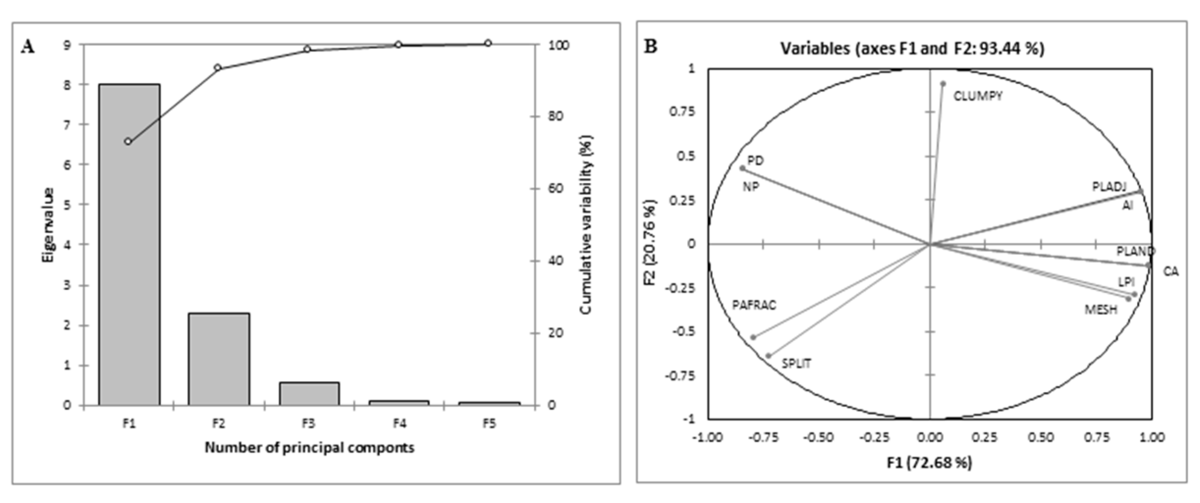
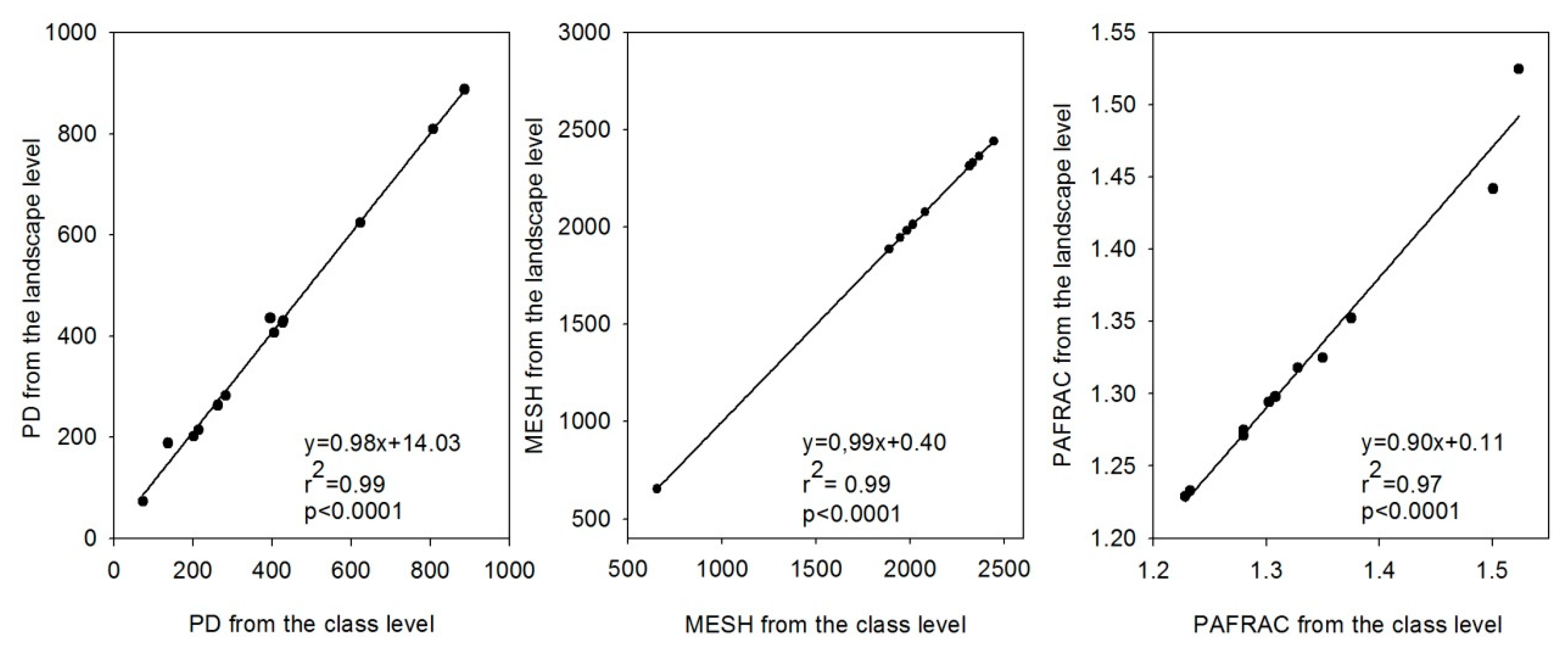
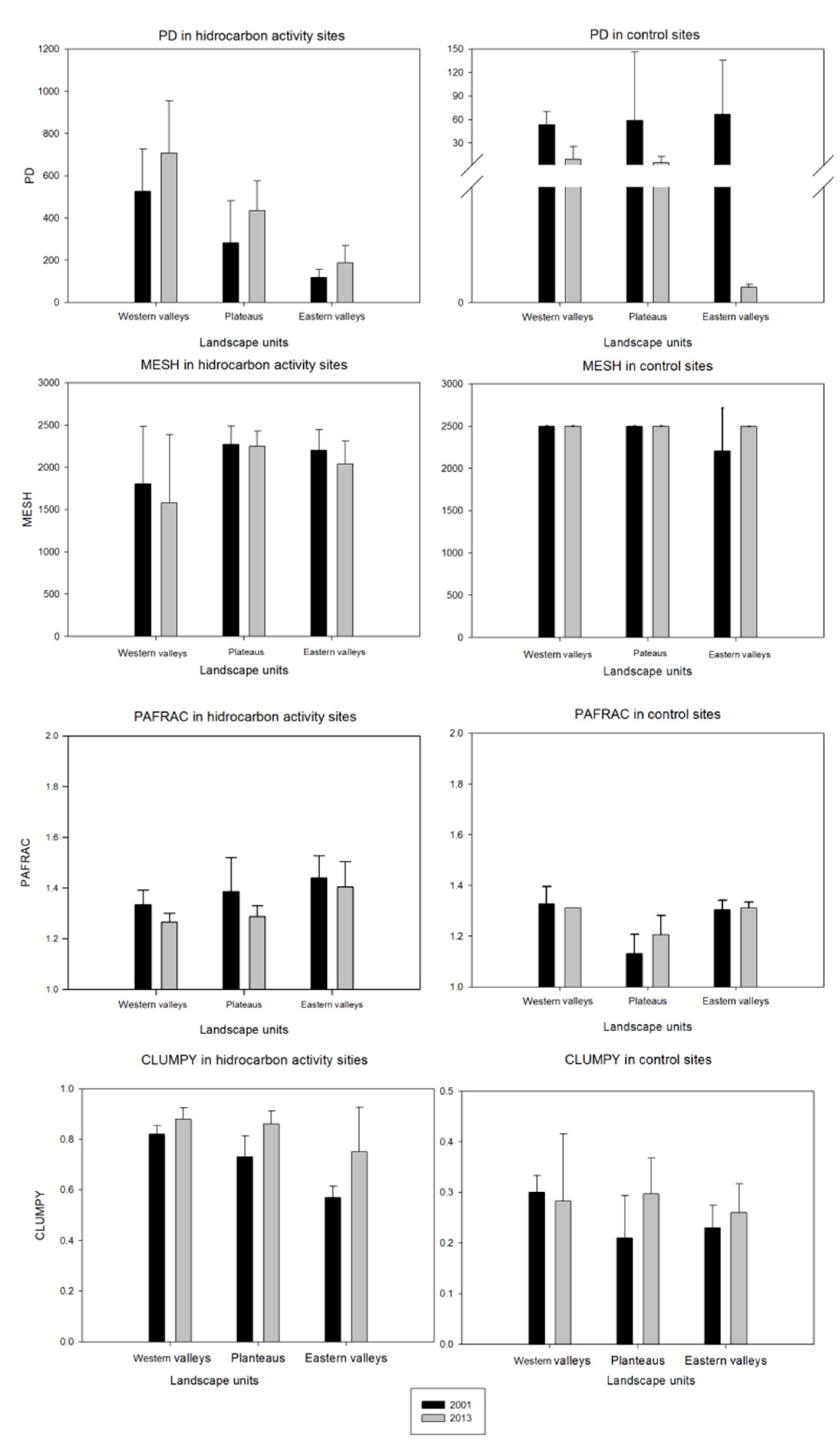
3.1. Analysis of Landscape Metrics at the Class Level

Figure 5 shows an example about elements on the landscape. This is a representative example about the impact of hydrocarbon activity on plateaus in the years 2001 and 2013.
Based on the obtained results, the CLUMPY metric was selected at the class level which explains 93.44% of the total variance (Figure 6, Table 1).
At the landscape level, PCA showed that factors 1 and 2 explain more than 95% of the total variance of the metrics analyzed (Figure 7, Table 2). From this analysis, the metrics selected were as follows: PD, MESH and PAFRAC, which are the ones that best explain the total variability in this case.
The correlation between the levels of analysis (class vs. landscape) was high and significant in all the analyzed metrics (Figure 8).
When resampling the satellite images, the ratio of the PD calculated with Landsat and SPOT images was significant and higher than 69% for the spatial resolutions of 10, 30 and 60 m. The PAFRAC showed a significant relationship higher than 82% for all the scales analyzed, and eventually, the MESH showed a relationship of 71% with a spatial resolution of 10 m, while when the resolution was 30 and 60 m the ratio was 95% and 74%, respectively (Figure 9).

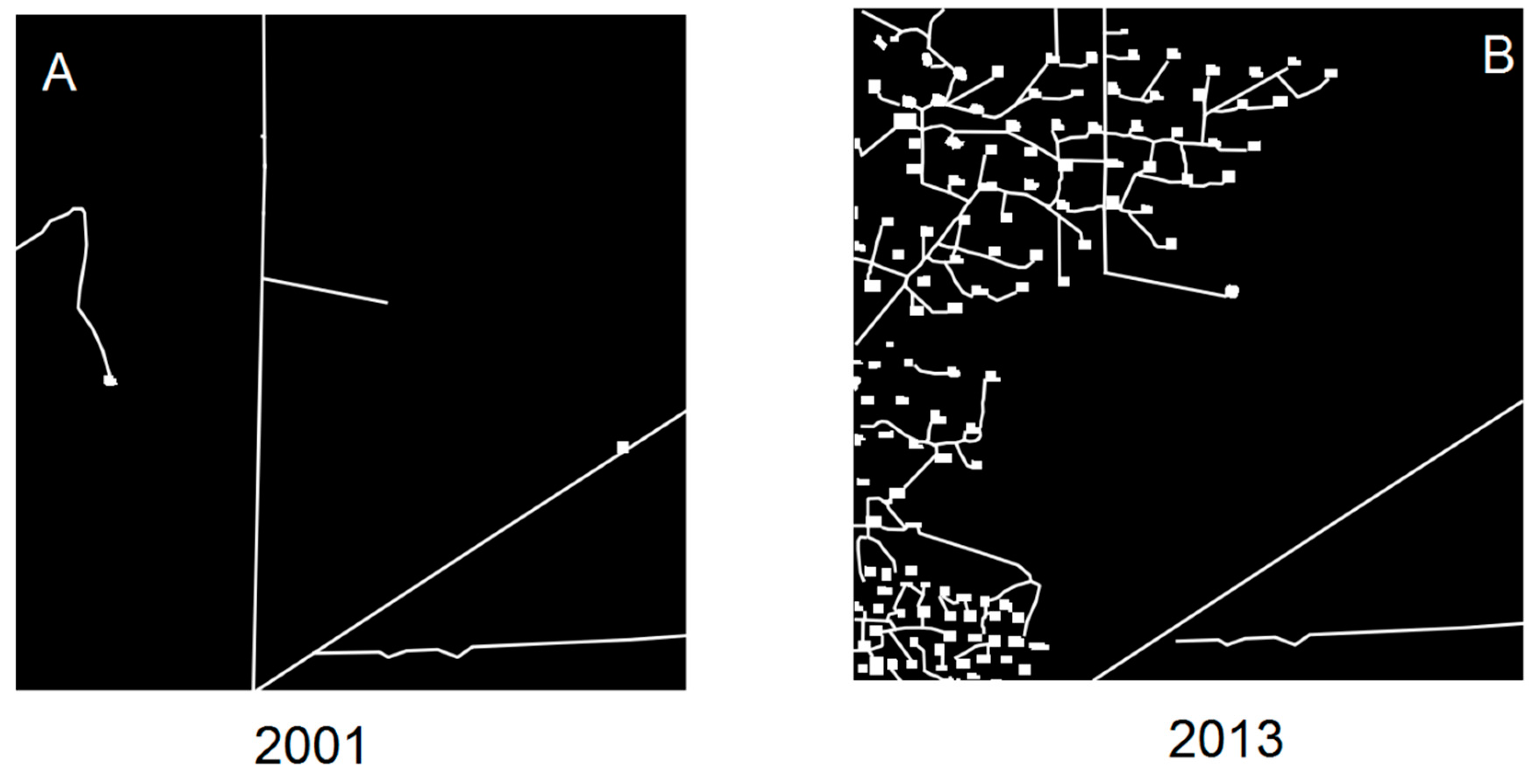
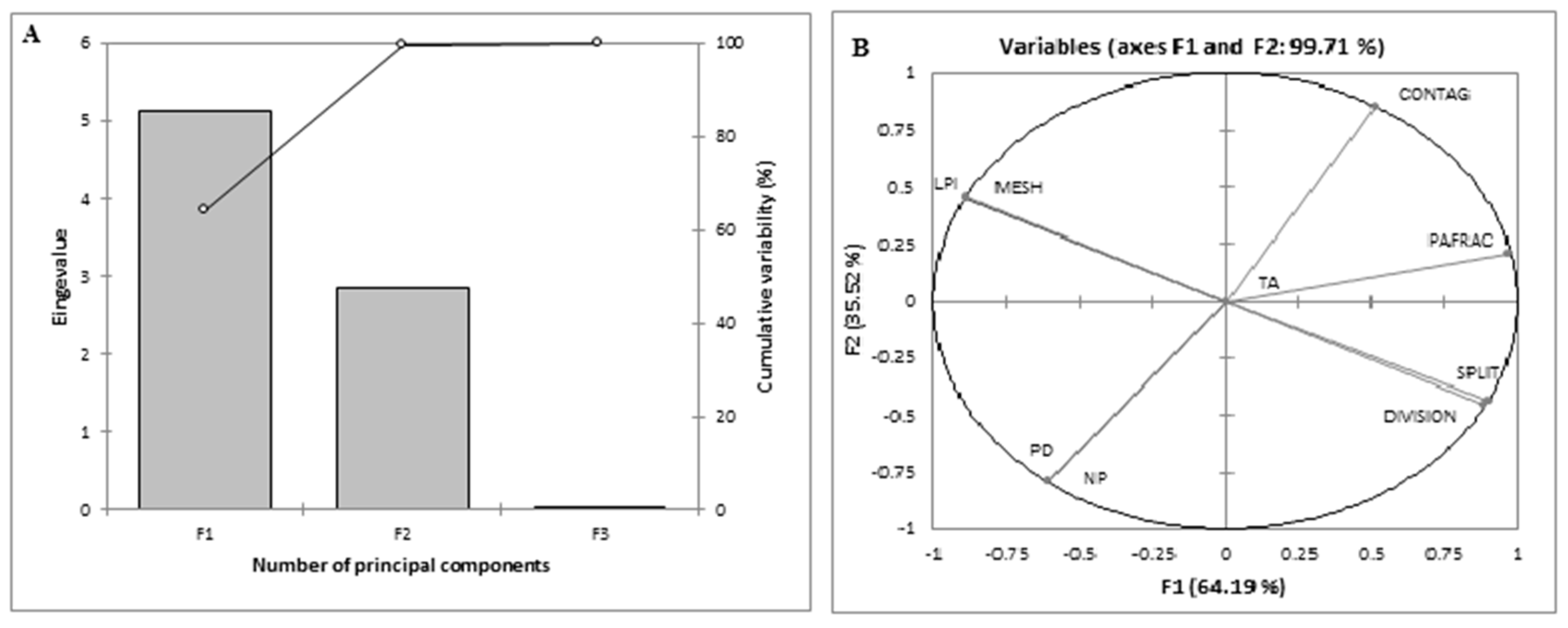
3.2. Analysis of the Temporal Change in Fragmentation

Between 2001 and 2013, fragmentation was greater at the sites with hydrocarbon activity than without (Figure 10). The average density of the patches in the landscape units went down from 60 to 14 patches per 100 hectares at the sites without any hydrocarbon activity between the years 2001 and 2013, whereas the mean density of patches increased from 309 to 444 patches at the sites with activity. The mean mesh size (MESH) remained constant between years in all three landscape units, whereas at the sites with oil production they decreased, mainly in the coastal valleys. The PAFRAC decreased in all three landscape units with hydrocarbon activity in the period analyzed, this decrease being more evident in the plateaus and the coastal valleys. On the other hand, this metric did not show a common pattern in the landscape units at the sites without any activity. CLUMPY showed an increase in all three landscape units between 2001 and 2013 at the sites with hydrocarbon activity. This increase was more evident in the coastal valleys. This metric did not show a common pattern of behavior in the landscape units at the control sites over time.

4. Discussion

Understanding and assessing trends in landscape fragmentation in arid and semi-arid zones can be achieved using metrics derived from spectral information. However, selecting and interpreting the minimum set of metrics that represent change most effectively is a challenge, since all metrics have limitations that restrict their use and application [52]. Multivariate analysis enables a reduction in the number of metrics by showing the redundancy between them. In this study, the metrics that best expressed the pattern of change in a Patagonian hydrocarbon basin were reduced to four from fourteen; several papers have focused on explaining the reduction of metrics for avoiding redundancy between them (e.g., [28,29,30,31]). The minimum package of metrics obtained in this study includes those that express form, like PAFRAC, aggregation such as CLUMPY and PD, and contagion and interspersion such as MESH. Form metrics measure the geometric complexity of a landscape, as well as the influence of the interaction between the shape and size of the patch on ecological processes. Aggregation metrics measure the tendency of patch types to be spatially aggregated which refers to the texture of the landscape. The contagion and interspersion metrics are based on adjacent patch types, considering information about border segments [46]. Numerous studies in the last two decades have reported on the behavior of landscape metrics; however, few have focused on changes in resolution [28]. Li and Wu [53] have shown that changes in the level of analysis could affect the behavior of the metrics. In this study, we show a high relationship between the metrics analyzed at both class and landscape levels (r2 > 0.97) and the scales (r2 > 0.69). This could be due to the fact that a binary classification was analyzed between an anthropogenic activity and a matrix without any disturbance, the latter being dominant in the landscapes irrespective of the scale.
Our results showed that the landscape units in the Patagonian hydrocarbon basin have undergone an important fragmentation process between 2001 and 2013. This loss of connectivity was more evident in the coastal valleys than in the rest of the landscape units. The first oil deposits in the region were located near to the coast at the beginning of the 20th century, in the costal valleys that descend to the sea from the upper terraced levels. The loss of connectivity was a consequence of hydrocarbon activity, since the applied metrics showed a tendency to fragmentation when compared with the control sites without any activity. This loss of connectivity, intensified in the analyzed period, facilitated the serious desertification process, caused by the mismanaging of the sheep grazing that occurred in the last century. The advance of desertification in the arid and semi-arid zones of Patagonia is one of the main socioecological and environmental problems present. The fragmentation of the plant cover matrix in the hydrocarbon basin under study can affect ecosystem functional and structural attributes such as increased runoff, diminished above-ground net primary productivity (and, consequently, secondary production), and increased physiognomic changes (e.g., replacement of grasslands by shrub-lands). This last aspect was already observed and measured in arid and semi-arid Patagonia were plant communities showed changes in land cover; in the western valleys the shrub-lands increased their coverage demonstrating the process of expansion of thickets of shrub plants in environments dominated by grasses or other herbaceous plants.
The probability that two animals located at two different points within the study area can be found without having to cross a barrier, such as a road or an urban area [49], decreased as a result of the oil activity; the MESH had a value close to 2500 ha in the control sites and of 1957 ha in the disturbed sites. The PD increased from 37 to 376 patches per 100 hectares at sites with hydrocarbon activity and it was observed that over time the forms had been simplified, as shown by PAFRAC, which decreased from a value of 1.38 to 1.31, possibly due to the increase in infrastructure and roads required by the petroleum industry. In the control sites, the temporal difference of the shape was not so marked, showing that there have been no modifications in the landscape configuration by the petroleum industry. CLUMPY showed that the patches are more aggregated in sites with hydrocarbon activity, which increased during the period analyzed. In the control sites, the aggregation between patches presented a random pattern. It should be noted that CLUMPY isolates the configuration component from the area component, thus giving an effective index of fragmentation that is not confused with changes in the area [21]. Between 2003 and 2004 there was an increase in the international price of a barrel of crude oil, and a consequent increase in oil exploitation, which is reflected in the opening of new locations, roads and tracks. This is due to the oil boom that has occurred since 2003 in the hydrocarbon basin in the Chubut province, as part of neo-extractivism and an era of well-being and prosperity that has had repercussions on the configuration of the regional landscape [54].

5. Conclusions

As a whole, this study showed that landscape is a complex system, with dynamics, spatial configuration, structure and functionality that are the result of the interaction between natural, economic and socio-cultural factors. In particular, in this paper, landscape fragmentation rates were quantitatively assessed in the hydrocarbon basin, located in the Chubut and Santa Cruz provinces of the arid and semi-arid zones of Patagonia (Argentina). It is important to measure and document fragmentation in the landscape, to support mitigation strategies, sustainable planning and policy development for hydrocarbon activity.
The fragmentation rates were herein evaluated over a period of twelve years, in three landscape units, using PCA to select the smallest package of metrics that best explain the fragmentation process. The minimum package of metrics obtained in this study includes those that express form, like PAFRAC, aggregation such as CLUMPY and PD, and contagion and interspersion such as MESH. The advantages of the methodology herein adopted is the use of a supervised classification to evaluate and categorize the impacts produced by the oil industry. The disadvantage is mainly linked with the binary approach which does not allow the inclusion of different land use and land cover types. As a future project, it would be interesting to include information on the combination of different land uses and land covers and, moreover, further research should be extended to consider the fragmentation of the landscape from an interdisciplinary perspective including the relationship between cultural and natural landscapes.

Author Contributions

Conceptualization, M.B and B.R.; methodology, M.B. and B.R.; software, M.B.; validation, M.B., B.L. and L.G.; formal analysis, M.B.; investigation, M.B.; resources, M.B.; data curation, M.B.; writing—original draft preparation, B.R., L.G. and R.L.; writing—review and editing, B.R.; visualization, R.L.; supervision, B.R.; project administration, M.B. and B.R.; funding acquisition, M.B. and B.R.

Funding

This research was supported on a National Scientific and Technical Research Council of Argentina (CONICET) doctoral fellowship (M. Buzzi) and was partially funded by the Argentinian Spatial Agency (CONAE, acronym in Spanish), which provided the satellite images of the SPOT 5.

Acknowledgments

We would like to thank the anonymous reviewers for their valuable comments of a previous draft.

Conflicts of Interest

The authors declare no conflicts of interest.

Appendix A

Table A1. Definition and description of FRAGSTATS metrics [29].
Landscape MetricDescriptionRangeUnitsFormula
Total Area (TA)TA equals the sum of the areas (m2) of all patches of the corresponding patch type, divided by 10,000 (to convert to hectares); that is, total class area.TA ≥ 0Ha. TA = j = l n aij
Clumpiness Index (CLUMPY)Equals the proportional deviation of the proportion of like adjacencies involving the corresponding class from that expected under a spatially random distribution. −1 ≥ CLUMPY ≤ 1None. G i = ( G ii k = l m g ik )
C L U M P Y = [ G i P i 1 P i si   G i   P i G i P i 1 P i   si   G i   < P i ; P i 0 , 5 P i G i P i si   G i   < P i ; P i < 0 , 5 ]
Gii = Number of like adjacencies (joins) between pixels of patch type (class) i based on the double-count method.
gik = Number of adjacencies (joins) between pixels of patch types (classes) i and k based on the double-count method.
Pi = Proportion of the landscape occupied by patch type (class) i.
Aggregation Index (AI)Aggregation index is calculated from an adjacency matrix, which shows the frequency with which different pairs of patch types (including like adjacencies between the same patch type) appear side-by-side on the map.0 ≦ AI ≦ 100Percent. AI = [ g ii max g ii ] ( 100 )
gii = Number of like adjacencies (joins) between pixels of patch type (class) i based on the single-count method.
max-gii = Maximum number of like adjacencies (joins) between pixels of patch type (class) i based on the single-count method.
Percentage of Landscape (PLAND)PLAND equals the sum of the areas (m2) of all patches of the corresponding patch type, divided by total landscape area (m2), multiplied by 100 (to convert to a percentage).0 ≥ PLAND ≤ 100Percent. PLAND = P i = j = i n a ij A ( 100 )
Pi = Proportion of the landscape occupied by patch type (class) i.
aij = Area (m2) of patch ij.
A = Total landscape area (m2).
Total class area (CA)Equals the sum of the areas (m2) of all patches of the corresponding patch type, divided by 10,000 (to convert to hectares).CA > 0Ha CA = j = l n a ij   ( 1 10000 )
aij = Area (m2) of patch ij.
Largest Patch Index (LPI)LPI equals the percentage of the landscape comprised by the largest patch.0 < LPI ≤ 100Percent LPI = max j = l ( a ij ) A (100)
aij = Area (m2) of patch ij.
A = Total landscape area (m2).
Effective Mesh Size (MESH)Equals the sum of patch area squared, summed across all patches of the corresponding patch type, divided by the total landscape area (m2), divided by 10,000 (to convert to hectares).Ratio of cell size to landscape area ≤ MESH ≤ total landscape area.Ha MESH = i = l m j = l m a   ij 2 A
aij = Area (m2) of patch ij.
A = Total landscape area (m2).
Perimeter-Area Fractal Dimension (PAFRAC)PAFRAC approaches one for shapes with very simple perimeters such as squares, and approaches 2 for shapes with highly convoluted, plane-filling perimeters.1 ≤ PAFRAC ≤ 2None P A F R A C =
2 [ N i = l m j = l m ( lnp ij   × lna ij   ) ] [ ( i = l m j = l m ( lnp ij   ) ( i = l m j = l m ( lna ij   ) ) ) ] ( N i = l m j = l m lnp ij 2 ) ( N i = l m j = l m lnp ij ) 2
aij = Area (m2) of patch ij.
pij = Perimeter (m) of patch ij.
N = Total number of patches in the landscape.
Splitting Index (SPLIT)SPLIT equals the total landscape area (m2) squared divided by the sum of patch area (m2) squared, summed across all patches in the landscape.1 ≤ SPLIT ≤ number of cells in the landscape squaredNone. SPLIT = A 2 j = 1 n a ij 2
Landscape Division Index (DIVISION)DIVISION equals one minus the sum of patch area (m2) divided by total landscape area (m2), quantity squared, summed across all patches of the corresponding patch type.0 ≤ DIVISION < 1Proportion. DIVISION = [ 1 j = l n ( a ij A ) 2 ]
aij = Area (m2) of patch ij.
A = Total landscape area (m2).aij = Area (m2) of patch ij.
A = Total landscape area (m2).
Number of Patches (NP)NP is the total number of patches in the landscape.NP ≥ 1None. NP = n i
ni = Number of patches in the landscape of patch type (class) i.
Patch Density (PD)PD equals the number of patches in the landscape, divided by total landscape area (m2), multiplied by 10,000 and 100 (to convert to 100 hectares).PD > 0Number per 100 hectares. PD = n i A ( 100 )
N = Total number of patches in the landscape.
A = Total landscape area (m2).
Percentage of Like Adjacencies (PLADJ)PLADJ equals the number of like adjacencies involving the focal class, divided by the total number of cell adjacencies involving the focal class; multiplied by 100 (to convert to a percentage). 0 ≤ PLADJ ≥ 100Percent. PLADJ = ( g ii k = l m g ik ) ( 100 )
gii = Number of like adjacencies (joins) between pixels of patch type (class) i based on the double-count method.
gik = Number of adjacencies (joins) between pixels of patch types (classes) i and k based on the double-count method.
Contagion Index (CONTAG)The observed contagion over the maximum possible contagion for the given number of patch types. Note, CONTAG considers all patch types present on an image, including any present in the landscape border, if present, and considers like adjacencies (i.e., cells of a patch type adjacent to cells of the same type). CONTAG considers all patch types present on an image, including any present in the landscape border, if present, and considers like adjacencies (i.e., cells of a patch type adjacent to cells of the same type).0 < CONTAG ≥ 100Percent. CONTAG = [ 1 + i = l m k = l m [ P i g ik k = l m g ik ] [ ln ( P i g ik k = l m g ik ) ] 2 ln ( m ) ] ( 100 )
Pi = Proportion of the landscape occupied by patch type (class) i.
gik = Number of adjacencies (joins) between pixels of patch types (classes) i and k based on the double-count method.
m = Number of patch types (classes) present in the landscape, including the landscape border if present.

References

  1. Sánchez, B.; Baena, C.; Esqueda, P. El entorno económico del sector y su importancia en Venezuela y el mundo. In La Competitividad de la Industria Petrolera Venezolana; CEPAL: Santiago de Chile, Chile, 2000; p. 76. [Google Scholar]
  2. Instituto Argentino de Petróleo y Gas IAPG. Suplemento Estadístico Petrotecnia; Instituto Argentino de Petróleo y Gas IAPG: Chubut, Argentina, 2018; p. 114. [Google Scholar]
  3. Instituto Argentino de Petróleo y Gas IAPG. La Industria Argentina de los Hidrocarburos; Informe Técnico; Instituto Argentino de Petróleo y Gas IAPG: Chubut, Argentina, 2015; p. 16. [Google Scholar]
  4. Paris de Ferrere, M. Inyección de agua y gas en yacimientos petrolíferos; Ediciones Astro Dala SA: Maracaibo, Venezuela, 2001; p. 390. [Google Scholar]
  5. Epstein, P.R.; Selber, J.; Borasin, S.; Foster, S.; Jobarteh, K.; Link, N. A life cycle analysis of its health and environmental impacts. In The Center for Health and the Global Environment; Harvard Medial School: Boston, MA, USA, 2002; p. 7. [Google Scholar]
  6. Ciano, N. Rehabilitación de áreas degradadas por la actividad petrolera. In Restauración Ecológica en la Diagonal Árida de la Argentina; Pérez, D.R., Rovere, A.E., Rodriguez Araujo, M.E., Eds.; Vazquez Massini: Buenos Aires, Argentina, 2013; pp. 261–267. [Google Scholar]
  7. Christie, K.S.; Jensen, W.F.; Schmidt, J.H.; Boyce, M.S. Long-term changes in pronghorn abundance index linked to climate and oil development in North Dakota. Biol. Conserv. 2015, 192, 445–453. [Google Scholar] [CrossRef]
  8. Pierre, J.P.; Wolaver, B.D.; Labay, B.J.; LaDuc, T.J.; Duran, C.M.; Ryberg, W.A.; Andrews, J.R. Comparison of recent oil and gas, wind energy, and other anthropogenic landscape alteration factors in Texas through 2014. Environ. Manag. 2018, 61, 805–818. [Google Scholar] [CrossRef] [PubMed]
  9. Birdsall, J.L.; McCaughey, W.; Runyon, J.B. Roads impact the distribution of noxious weeds more than restoration treatments in a lodgepole pine forest in Montana, USA. Restor. Ecol. 2012, 20, 517–523. [Google Scholar] [CrossRef]
  10. Milt, A.W.; Gagnolet, T.D.; Armsworth, P.R. The costs of avoiding environmental impacts from shale-gas surface infrastructure. Conserv. Biol. 2016, 30, 1151–1158. [Google Scholar] [CrossRef]
  11. Forman, R.T.T. Land Mosaics: The Ecology of Landscapes and Regions; Island Press: Cambridge, UK, 1995. [Google Scholar]
  12. With, K.A.; Gardner, R.H.; Turner, M.G. Landscape connectivity and population distributions in heterogeneous environments. Oikos 1997, 78, 151–169. [Google Scholar] [CrossRef]
  13. Taylor, P.D.; Fahrig, L.; Henein, K.; Merriam, G. Connectivity is a vital element of landscape structure. Oikos 1993, 68, 571–573. [Google Scholar] [CrossRef]
  14. Luque, S.; Saura, S.; Fortin, M.J. Landscape connectivity analysis for conservation: Insights from combining new methods with ecological and genetic data. Landsc. Ecol. 2012, 27, 153–157. [Google Scholar] [CrossRef]
  15. Ziółkowska, E.; Ostapowicz, K.; Radeloff, V.C. Effects of different matrix representations and connectivity measures on habitat network assessments. Landsc. Ecol. 2014, 29, 1551–1570. [Google Scholar] [CrossRef] [Green Version]
  16. Zimbres, B.; Furtado, M.M.; Jácomo, A.T.; Silveira, L.; Sollmann, R.; Tôrres, N.M.; Machado, R.B.; Marinho-Filho, J. The impact of habitat fragmentation on the ecology of xenarthrans (Mammalia) in the Brazilian Cerrado. Landsc. Ecol. 2013, 28, 259–269. [Google Scholar] [CrossRef]
  17. MacArthur, R.H.; Wilson, E.O. The Theory of Island Biogeography; Princeton University: Princeton, NJ, USA, 1967. [Google Scholar]
  18. Fahrig, L.; Baudry, J.; Brotons, L.; Burel, F.G.; Crist, T.O.; Fuller, R.J.; Sirami, C.; Siriwardena, G.M.; Martin, J.L. Functional landscape heterogeneity and animal biodiversity in agricultural landscapes. Ecolo. Lett. 2011, 14, 101–112. [Google Scholar] [CrossRef]
  19. Herrera, L.; Laterra, P. Relaciones entre la riqueza y composición florística con el tamaño de fragmentos de pastizales en la Pampa Austral, Argentina. In Panorama de la Ecología de Paisajes en Argentina y en Países Sudamericanos; Matteucci, S., Ed.; Ediciones INTA: Buenos Aires, Argentina, 2007; pp. 383–396. [Google Scholar]
  20. Herrera, L.; Laterra, P. Relative influence of size, connectivity and disturbance history on plant species richness and assemblages in fragmented grasslands. Appl. Veg. Sci. 2011, 14, 181–188. [Google Scholar] [CrossRef]
  21. Olsoy, P.J.; Zeller, K.A.; Hicke, J.A.; Quigley, H.B.; Rabinowitz, A.R.; Thornton, D.H. Quantifying the effects of deforestation and fragmentation on a range-wide conservation plan for jaguars. Biol. Conserv. 2016, 203, 8–16. [Google Scholar] [CrossRef]
  22. Pincheira-Ulbrich, J.; Rau, J.R.; Peña Cortés, F. Patch size and shape and their relationship with tree and shrub species richness. Phyton 2009, 78, 121–128. [Google Scholar]
  23. Li, S.; Yang, B. Introducing a new method for assessing spatially explicit processes of landscape fragmentation. Ecol. Indic. 2015, 56, 116–124. [Google Scholar] [CrossRef]
  24. Peng, Y.; Mi, K.; Qing, F.; Xue, D. Identification of the main factors determining landscape metrics in semi-arid agro-pastoral ecotone. J. Arid Environ. 2016, 124, 249–256. [Google Scholar] [CrossRef]
  25. Heller, N.E.; Zabaleta, E.S. Biodiversity management in the face of climate change: A review of 22 years of recommendations. Biol. Conserv. 2009, 142, 14–32. [Google Scholar] [CrossRef]
  26. Read, J.; Lam, N.S. Spatial methods for characterizing land cover and detecting land cover changes for the tropics. Int. J. Remote Sens. 2002, 23, 2457–2474. [Google Scholar] [CrossRef]
  27. Sinha, P.; Kumar, L.; Reid, N. Rank-based methods for selection of landscape metrics for land cover pattern change detection. Remote Sens. 2016, 8, 107. [Google Scholar] [CrossRef]
  28. Cushman, S.A.; McGarigal, K.; Neel, M.C. Parsimony in landscape metrics: Strength, universality, and consistency. Ecol. Indic. 2008, 8, 691–703. [Google Scholar] [CrossRef]
  29. Plexida, S.G.; Sfougaris, A.I.; Ispikoudis, I.P.; Papanastasis, V.P. Selecting landscape metrics as indicators of spatial heterogeneity—A comparison among Greek landscapes. Int. J. Appl. Earth Observ. Goinform. 2014, 26, 26–35. [Google Scholar] [CrossRef]
  30. Stanfield, B.J.; Bliss, J.C.; Spies, T.A. Land ownership and landscape structure: A spatial analysis of sixty-six Oregon (USA) Coast Range watersheds. Landsc. Ecol. 2002, 17, 685–697. [Google Scholar] [CrossRef]
  31. Abdi, H.; Williams, L.J. Principal component analysis. Wiley Interdiscip. Rev Comput. Stat. 2010, 2, 433–459. [Google Scholar] [CrossRef]
  32. McGarigal, K.; Cushman, S.A.; Neel, M.C.; Ene, E. FRAGSTATS: Spatial Pattern Analysis Program for Categorical Maps. Computer Software Program Produced by the Authors at the University of Massachusetts Amherst. 2002. Available online: https://www.umass.edu/landeco/research/fragstats/fragstats.html (accessed on 25 January 2018).
  33. Paruelo, J.M.; Aguiar, M.R. Impacto humano sobre los ecosistemas. El caso de la desertificación. Cienc. Hoy 2003, 13, 48–59. [Google Scholar]
  34. Ares, J.; Bertiller, M.; Bisigato, A. Modeling and measurement of structural changes at a landscape scale in dryland areas. Environ Model Assess. 2003, 8, 1–13. [Google Scholar] [CrossRef]
  35. Bond, W.J. Large parts of the world are brown or black: A different view on the ‘Green World’ hypothesis. J. Veg. Sci. 2005, 16, 261–266. [Google Scholar] [CrossRef]
  36. Merino, M.L.; Carpinetti, B.N.; Abba, A.M. Invasive mammals in the National Parks system of Argentina. Nat. Areas J. 2009, 29, 42–49. [Google Scholar] [CrossRef]
  37. Raffaele, E.; Veblen, T.T.; Blackhall, M.; Tercero-Bucardo, N. Synergistic influences of introduced herbivores and fire on vegetation change in northern Patagonia, Argentina. J. Veg. Sci. 2011, 22, 59–71. [Google Scholar] [CrossRef]
  38. Cheli, G.H.; Pazos, G.E.; Flores, G.E.; Corley, J.C. Efecto de los gradientes de pastoreo ovino sobre la vegetación y el suelo en Península Valdés, Patagonia Argentina. Ecol. Austral 2016, 26, 200–211. [Google Scholar]
  39. Svampa, M.; Viale, E. Maldesarrollo: La Argentina del Extractivismo y el Despojo; Katz Editores: Buenos Aires, Argentina, 2015; pp. 15–36. [Google Scholar]
  40. Instituto Nacional de Estadísticas y Censos INDEC, Censo. Resultados Previsionales. IOP Publishing PhysicsWeb. 2010. Available online: http://www.indec.gov.ar/ (accessed on 26 June 2016).
  41. León, R.J.C.; Bran, D.; Collantes, M.; Paruelo, J.M.; Soriano, A. Grandes unidades de vegetación de la Patagonia extra andina. Ecol. Austral 1998, 8, 125–144. [Google Scholar]
  42. Servicio Meteorológico Nacional SMN. Available online: http://www3.smn.gov.ar/serviciosclimaticos/?mod=elclima&id=3 (accessed on 19 June 2019).
  43. Fan, C.; Myint, S. A comparison of spatial autocorrelation indices and landscape metrics in measuring urban landscape fragmentation. Landsc. Urban Plan. 2014, 121, 117–128. [Google Scholar] [CrossRef]
  44. Quantum GIS Development Team. Quantum GIS Geographic Information System. Open Source Geospatial Foundation Project. 2016. Available online: http://qgis.osgeo.org (accessed on 19 January 2018).
  45. Wang, X.; Blanchet, F.G.; Koper, N. Measuring habitat fragmentation: An evaluation of landscape pattern metrics. Methods Ecol. Evol. 2014, 5, 634–646. [Google Scholar] [CrossRef]
  46. Feng, Y.; Liu, Y. Fractal dimension as an indicator for quantifying the effects of changing spatial scales on landscape metrics. Ecol. Indic. 2015, 53, 18–27. [Google Scholar] [CrossRef]
  47. Moser, B.; Jaeger, J.A.; Tappeiner, U.; Tasser, E.; Eiselt, B. Modification of the effective mesh size for measuring landscape fragmentation to solve the boundary problem. Landsc. Ecol. 2007, 22, 447–459. [Google Scholar] [CrossRef]
  48. Jaeger, J. Landscape division, splitting index, and effective mesh size: New measures of landscape fragmentation. Landsc. Ecol. 2000, 15, 115–130. [Google Scholar] [CrossRef]
  49. Schmiedel, I.; Culmsee, H. The influence of landscape fragmentation, expressed by the “Effective Mesh Size Index”, on regional patterns of vascular plant species richness in Lower Saxony, Germany. Landsc. Urban Plan. 2016, 153, 209–220. [Google Scholar] [CrossRef]
  50. Liu, Y.; Wei, X.; Li, P.; Li, Q. Sensitivity of correlation structure of class- and landscape-level metrics in three diverse regions. Ecol. Indic. 2016, 64, 9–19. [Google Scholar] [CrossRef]
  51. Lausch, A.; Herzog, F. Applicability of landscape metrics for the monitoring of landscape change: Issues of scale, resolution and interpreatability. Ecol. Indic. 2002, 2, 3–15. [Google Scholar] [CrossRef]
  52. European Environment Agency EEA. What is landscape fragmentation? In Landscape Fragmentation in Europe; European Environment Agency: Luxembourg; Copenhagen, Denmark, 2011; pp. 9–19. [Google Scholar] [CrossRef]
  53. Li, H.; Wu, J. Use and misuse of landscape indices. Lands. Ecol. 2004, 9, 389–399. [Google Scholar] [CrossRef]
  54. Peters, S. Poscrecimiento y Buen Vivir: ¿Discursos políticos alternativos o alternativas políticas? In Post-Crecimiento y BuenVivir. Propuestas Globales Para la Construcción de Sociedades Equitativas y Sustentables; Gustavo, E., Ed.; Friedrich-Ebert-Stiftung (FES): Quito, Ecuador, 2016; pp. 123–161. [Google Scholar]
Figure 1. (A): Location of Argentina (in red study area). (B): Location of the study area and the selected sampling sites with and without hydrocarbon activity.
Sustainability 11 05956 g001
Figure 2. Oilfields (rectangular clearings) with hydrocarbon activity on coastal valleys (courtesy of Alejandro Tula).
Sustainability 11 05956 g002
Figure 3. Diagram of the methodology used.
Sustainability 11 05956 g003
Figure 4. (A) Natural vegetation in coastal valleys (Colliguaja intergerrima and Retanilla patagonica). (B) Natural vegetation in plateaus (Pappostipa speciosa, Pappostipa humilis and Poa spiciformis). (C) Natural vegetation in eastern valleys (Nassauvia glomerulosa and Chuquiraga avellanedae).
Sustainability 11 05956 g004
Figure 5. In white, the linear and no-linear elements in the plateaus are shown.
Sustainability 11 05956 g005
Figure 6. Scree plot (A) shows the eigenvalue and cumulative variability (%). The correlation circle (B) shows a projection of the initial variables in the factors space. Panels A and B show the results of principal component analysis (PCA) at the class level.
Sustainability 11 05956 g006
Figure 7. Scree plot (A) shows the eigenvalue and the cumulative variability (%). The correlation circle (B) shows a projection of the initial variables in the factors space. The panels A and B show the results of PCA at the landscape level.
Sustainability 11 05956 g007
Figure 8. Correlation analysis between the levels of analysis (class vs. landscape).
Sustainability 11 05956 g008
Figure 9. Regression analysis between Landsat and SPOT images corresponding to patch density (PD), perimeter-area fractal dimension (PAFRAC), and effective mesh size (MESH) metrics with different spatial resolution. PD (number of patches/100 ha), PAFRAC (proportion), MESH (ha).
Sustainability 11 05956 g009
Figure 10. Graphs showing the results of the metrics at the landscape level, including the standard deviation.
Sustainability 11 05956 g010
Table 1. Total variance explained analysis at the class level.
F1F2F3F4F5
Eigenvalue7.992.280.560.100.05
Variability (%)72.6720.765.150.940.46
F: Factor analysis.
Table 2. Total variance explained analysis at the landscape level.
F1F2F3
Eigenvalue5.132.840.02
Variability (%)64.1935.510.29
F: Factor analysis.

