Application of Artificial Intelligence Techniques to Predict the Well Productivity of Fishbone Wells

Abstract

Fishbone multilateral wells are applied to enhance well productivity by increasing the contact area between the bottomhole and reservoir region. Fishbone wells are characterized by reduced operational time and a competitive cost in comparison to hydraulic fracturing operations. However, limited models are reported to determine the productivity of fishbone wells. In this paper, several artificial intelligence methods were applied to estimate the performance of fishbone wells producing from a heterogeneous and anisotropic gas reservoir. The well productivity was determined using an artificial neural network, a fuzzy logic system and a radial basis network. The models were developed and validated utilizing 250 data sets, with the inputs being the permeability ratio (K_h/K_v), flowing bottomhole pressure and lateral length. The results showed that the artificial intelligence models were able to predict the fishbone well productivity with an acceptable absolute error of 7.23%. Moreover, a mathematical equation was extracted from the artificial neural network, which is able to provide a simple and direct estimation of fishbone well productivity. Actual flow tests were used to evaluate the reliability of the developed model, and a very acceptable match was obtained between the predicted and actual flow rates, wherein an absolute error of 6.92% was achieved. This paper presents effective models for determining the well performance of complex multilateral wells producing from heterogeneous reservoirs. The developed models will help to reduce the uncertainty associated with numerical methods, and the extracted equation can be inserted into commercial software, thereby significantly reducing deviation between the actual data and simulated results.

1. Introduction

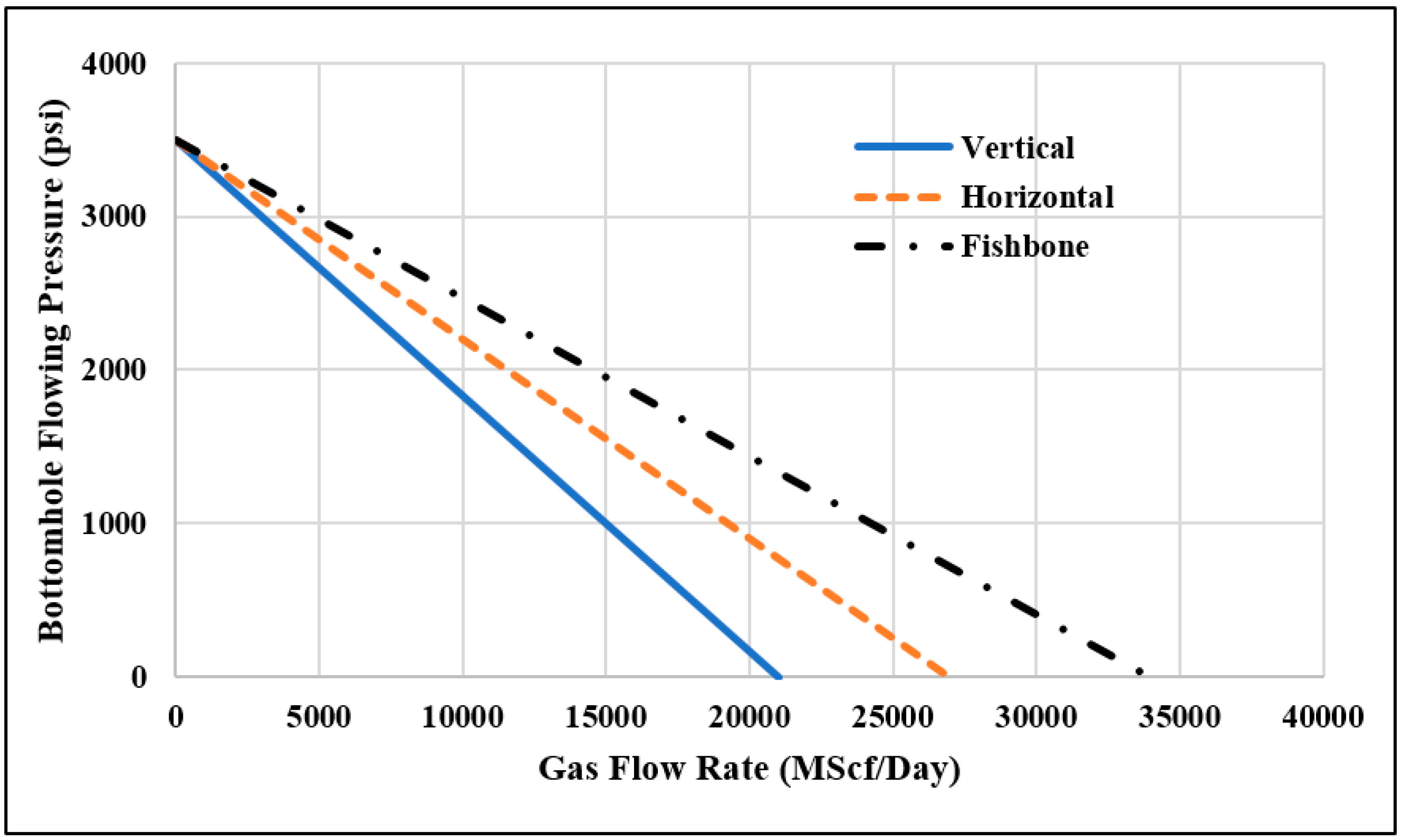
A multilateral well is defined as a well with multiple branches in the lower bore-hole targeting the pay zone in the same layer or different layers. Depending on the main well bore, a multilateral well can be classified as a root well or a fishbone well. For a root well, the main well bore is vertical, while for a fishbone well the laterals are drilled out from a horizontal well bore [1]. Fishbone wells are applied to enhance well productivity by increasing the contact area between the bottomhole and reservoir region. The productivities of vertical, horizontal and fishbone wells are depicted in Figure 1. Fishbone wells are characterized by larger drainage area; consequently, higher production rates can be achieved compared to vertical and horizontal wells [2]. In comparison to hydraulic fracturing operations, fishbones require less operational time and incur less expense [3]. Furthermore, fishbone wells have shown better performance than fractured horizontal wells in producing from tight reservoirs [2].

Predicting the well productivity is an essential factor in designing and completing a production well, as well as selecting the artificial lift and stimulation processes [4]. Several techniques have been reported to estimate the well performance for multilateral wells. Different correlations and analytical models have been developed to determine the inflow performance relationship (IPR), with the most popular equations being Fetkovitch’s and Vogel’s correlations [5,6]. Recently, numerical simulators have been utilized to estimate well productivity, which resulted in a significant reduction in estimation errors.

Fishbone wells can be considered a combination of different types of wells, such as horizontal, directional and multilateral. They have a complicated geometry and require complex models to predict their inflow performance. Therefore, several assumptions are generally applied to predict the performance of a fishbone well, such as neglecting the number of laterals or assuming constant pressure in all laterals. This leads to considerable estimation errors and significant deviations between the actual production data and predicted results.

This paper presents a new approach to determine the productivity of fishbone wells. Artificial intelligence techniques were utilized to develop predictive models and avoid the uncertainty of numerical methods. The developed models require the permeability ratio (K_h/K_v), flowing bottomhole pressure and lateral length to determine well productivity. The reliability of the developed models was verified using actual field data, wherein an absolute error of 6.92% was achieved for an ANN-based equation.

1.1. Inflow Performance Relationship

Borisov [7] proposed an analytical model to estimate the inflow performance relationship (IPR) for single phase multilateral wells. This model assumes steady state conditions, leading to impractical predictions. Therefore, Economides et al. [8] modified Borisov’s model by including pseudo steady state conditions. Furthermore, Salas et al. [9] investigated the impact of nearby damage (skin factor) on well productivity using different multilateral configurations. Furui et al. [5] developed an analytical model for fishbone multilateral wells. They concluded that the productivity can be expressed as a function of skin factor, drainage distance, permeability ratio and reservoir dimensions.

Yildiz [10] upgraded Salas and colleagues’ equation to model multilateral wells producing from extremely heterogeneous reservoirs. Guo et al. [4] reported that multilateral wells are involved with several flow regimes, including linear horizontal flow, radial flow, and vertical radial flow. Also, they mentioned that two different regions exist in the reservoir, the outer undrilled region and inner drilled region, with each region having a certain flow regime.

Yu et al. [11] used the net present value (NPV) concept to compare the performance of fishbone wells with that of fractured horizontal wells. They found that fishbone wells performed better than fractured horizontal wells, especially in tight reservoirs. The first attempt to couple the inflow performance with out-flow performance was reported by Lian et al. [12]. They developed a model by assuming uniform flow rate distribution, which is applicable in pseudo steady or unsteady flow state conditions.

In addition, different numerical models have been developed to simulate well productivity by treating each branch as a fracture with dimensions similar to the lateral dimensions. Several reservoir models have been evaluated to simulate dual porosity systems, triple porosity systems, and isotropic and anisotropic permeability conditions [13]. Moreover, computational fluid dynamics (CFD) analysis has been utilized to model the performance of fishbone wells in depleted reservoirs under water flooding operations. Fishbone multilateral wells have shown a productivity improvement of 25% in comparison with conventional horizontal wells during water flooding treatments [14].

Abdulazeem and Alnuaim [15] developed a new empirical model to determine the performance of a fishbone well in a homogeneous oil reservoir. Their model investigated the effects of reservoir permeability, porosity and fluid properties on the well’s productivity. They used Vogel’s model to validate the developed IPR fishbone model, and found that the developed model had a lower estimation error compared to Vogel’s model. Moreover, Ahmed et al. [6] extended the model proposed by Abdulazeem and Alnuaim in order to predict the performance of fishbone wells producing from gas reservoirs. They reported that their extended model was able to determine the gas production rate for a wide range of reservoir and well parameters. Also, they used real field data to verify their model’s reliability, with an acceptable match obtained between the actual data and predicted gas flow rates.

Al-Mashhad et al. [16] evaluated the performance of multilateral wells using an artificial neural network (ANN). Their ANN model was able to determine the oil production rate for multilateral wells based on reservoir and well parameters. They compared the developed model with several analytical models and empirical correlations. They found that the developed ANN model was capable of outperforming the other models, with strong matching between the actual and predicted flow rates achieved. Specifically, the model had an average absolute percentage error of 7.9%.

In this work, three artificial intelligence methods were utilized to predict the performance of fishbone wells. An artificial neural network, fuzzy logic system and radial basis function were used. The inputs to the models included the permeability ratio, flowing bottomhole pressure and lateral length. The developed models showed a strong predictive performance, with an acceptable absolute error of 7.23%. Also, a mathematical equation was extracted using the optimized ANN model. This extracted correlation provides a simple and direct estimation of the fishbone productivity. The ANN-based equation was verified using actual field data, wherein an absolute error of 6.92% was achieved.

1.2. Artificial Intelligence Techniques

The concept of artificial networks was introduced into engineering research in the 1940s [17,18]. In the early stages, artificial intelligence was used to solve complex equations and mimic the nervous system [19,20]. Artificial intelligence (AI) techniques include artificial neural networks, fuzzy logic systems, support vector machines and radial basis networks. Artificial neural networks (ANNs) are considered effective AI tools; therefore, they have been widely applied in several fields, such as in classification and optimization tasks [21,22]. An ANN model is a system of neurons and hidden layers [23]. Usually the whole data is grouped into two sets, namely the training and testing data sets. The training set is used to train the network and capture the relationship between the input and output parameters, while the testing data are used to measure the reliability of the developed ANN system. During the training stage, the testing data remain unseen by the model, which increases confidence in the model’s reliability [24,25,26]. A fuzzy logic model is an integrated network that combines a neural network with fuzzy logic. The most common model of fuzzy logic is an adaptive neuro-fuzzy inference system (ANFIS), which has the ability to extract the benefits of AI techniques in (a) single or multi-framework(s) [27]. Another kind of AI method is the radial basis function (RBF), which consists of linear and nonlinear functions [28].

Recently, artificial intelligence techniques have been extensively applied in the petroleum industry, especially in predicting well or field performance. Alajmi et al. [29] made predictions about choke performance using an ANN. Alarifi et al. [30] estimated the productivity index for horizontal oil wells using an ANN, a functional network and fuzzy logic. Chen et al. [31] applied a neural network and fuzzy logic to evaluate the performance of an inflow control device (ICD) in a horizontal well. Their model investigated the influence of reservoir parameters, such as reservoir size, thickness, heterogeneity and permeability ratio, on ICD completion performance.

Elkatatny et al. [32,33] comprehensively applied artificial neural networks (ANNs) to determine the permeability of a heterogeneous reservoir, and to estimate the rheological properties of drilling fluids based on real-time measurements. They developed robust models that can be used by petroleum engineers to obtain highly accurate predictions in less time. Van and Chon [34,35] evaluated the performance of CO₂ flooding using artificial neural network techniques. Specifically, they developed ANN models to determine the oil production rate, CO₂ production and gas oil ratio (GOR).

2. Data Acquisition and Analysis

In this work, the used data were generated by a commercial well performance software, with more than 250 runs performed. Real reservoir and well data were utilized as inputs for the commercial software. The minimum and maximum limits for each parameter were accurately selected. Then, the software outputs were carefully reviewed by a production consultant with over 30 years’ experience in the petroleum industry. Thereafter, the most practical results were used to develop the proposed models. The reservoir model was constructed in a 3D Cartesian grid system (62 × 21 × 11) with a fishbone well placed at the center. The dimensions of the reservoir were set to 20,000 ft (length) by 10,000 ft (width), with a depth of 750 ft. The reservoir was single layer, dry gas and anisotropic, and had produced for 20 years. The generated data, which comprised of more than 250 data sets, were sufficient to train and validate the artificial intelligence models. The data sets included simulation results for flowing bottomhole pressure (P_wf), well production rate, distances between laterals, length of each lateral, number of laterals, and permeability ratio (K_h/K_v).

A randomization function was utilized to divide the whole data into two sets: training and testing groups. The training data, which was 70% of the total data, was used to train the networks to capture the relationship between the inputs and flow rate. The testing data, which was data that was unseen during the training stage, was utilized to evaluate the reliability of the models. Before running the AI models, statistical analyses were conducted to determine their minimum, maximum, mean, mode and other statistical parameters, the results of which are summarized in

Table 1. A statistical analysis of the input/output data.

Parameter	Kh/Kv	No. of Laterals	Length (ft)	Distance (ft)	Pwf (psia)	Flow Rate (scf/D)
Minimum	1	2	700	1300	14.7	0
Maximum	1000	14	3100	5200	4800	197,903.226
Mean	61	6.667	2759.523	2723.809	2359.558	81,860.474
Mode	10	6	3100	2600	14.7	0
Range	999	12	2400	3900	4785.3	197,903.226
Standard Deviation	211.275	2.499	693.099	685.121	1551.738	48,712.516
Skewness	4.192	1.412	−1.9159	2.0689	0.09535	−0.118
Kurtosis	18.73	5.358	5.3081	9.503	1.7184	2.216
Coefficient of variation	346.352	37.491	25.116	25.153	65.763	59.507

. As shown in the table, the permeability ratio (K_h/K_v) ranged from 1 to 1000, while the flowing bottomhole pressure (P_wf) varied between 14.7 and 4800 psia. The statistical dispersion for flow rate results was measured by calculating the skewness and kurtosis, with the data showing huge spread over a wide range of values.

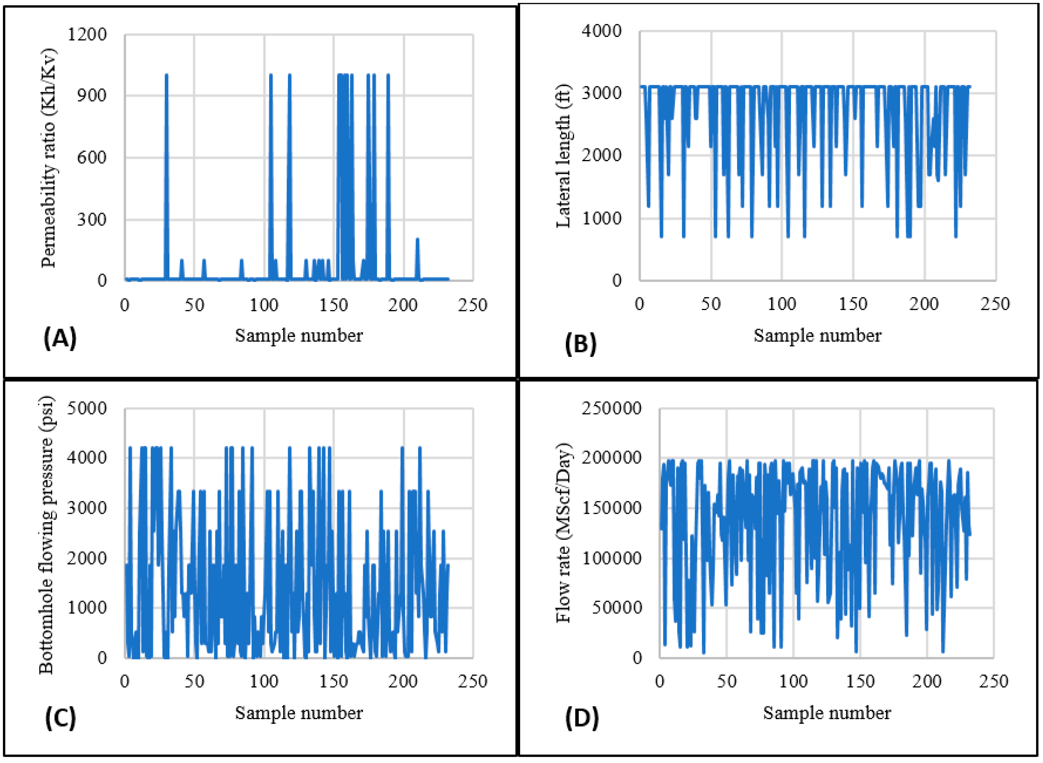
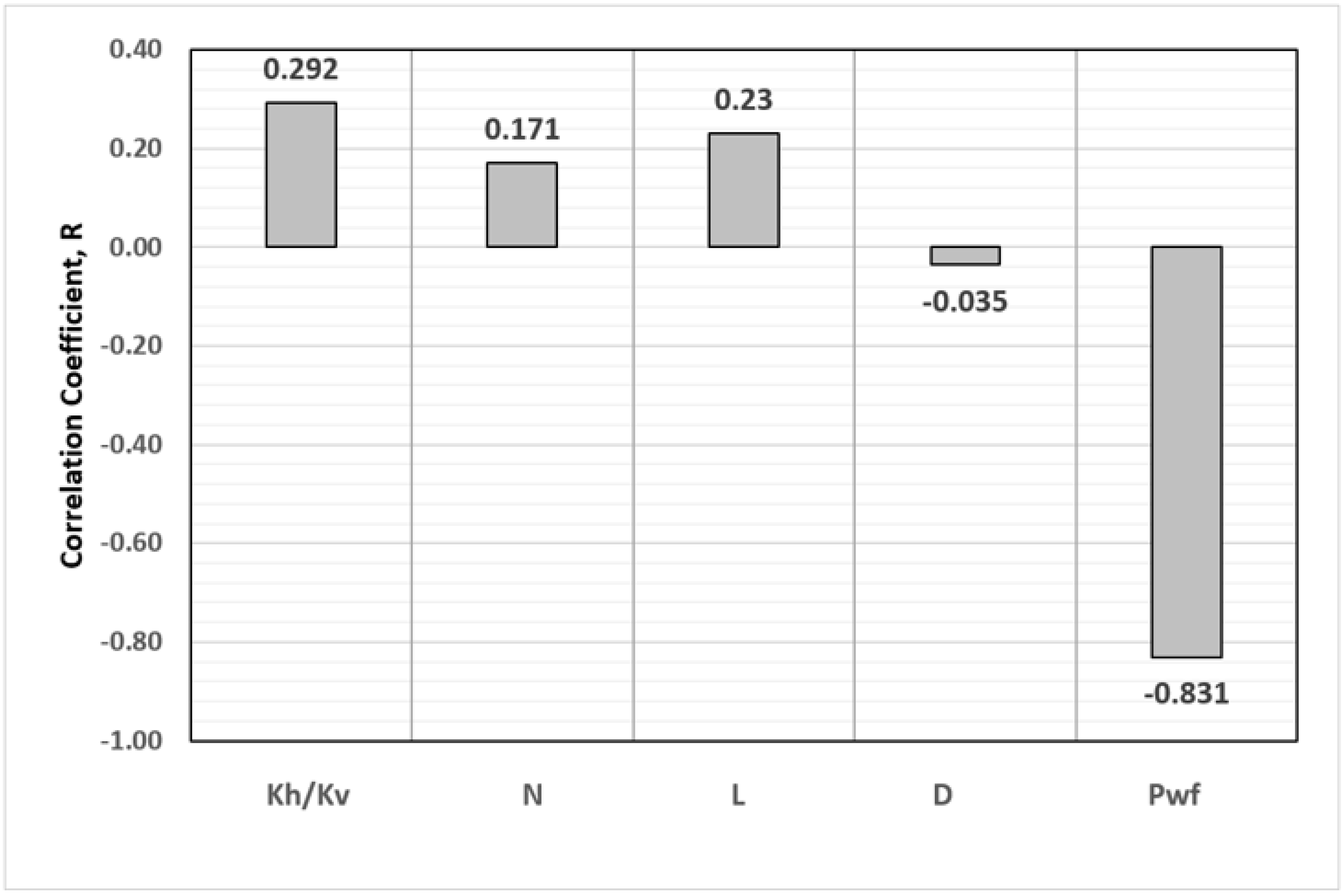
In addition, statistical distributions were obtained for all of the data to get a rough sense of the density of the underlying distributions, wherein the data set was found to represent a multimodal pattern. Figure 2 shows the distributions for input and output parameters against the number of samples. In general, the data showed typical trends for reservoir properties. For example, a hydrocarbon reservoir usually has one average permeability value, but it can produce using several bottomhole pressures. Therefore, one value can be used to represent the reservoir’s permeability, while a wide range of flowing pressures can be applied. Finally, correlation coefficients were determined to measure the impact of the input parameters on the well flow rate, as shown in Figure 3. Strong relationships were observed between the production rate and the flowing bottomhole pressure (P_wf), permeability ratio (K_h/K_v) and lateral length (L), with correlation coefficient values of −0.831, 0.292 and 0.230, respectively. The results of the correlation coefficient analysis indicate that the flow rate can be increased by reducing the flowing pressure or by increasing the lateral length. Also, increased hydrocarbon production can be obtained from a hydrocarbon reservoir with a higher permeability ratio. However, the number of laterals (N) and distance between laterals (D) showed very small correlation coefficient values (0.171 and −0.035, respectively). The same observation was reported by Ahmed et al. [6], who found that increasing the number of laterals or the distance between the laterals only had a minor effect on improving the fishbone productivity. Therefore, the number of laterals and the distance between laterals were excluded from further research as input parameters.

In summary, the statistical distribution plots indicated that most of the data set was represented by a multimodal pattern, while the correlation coefficient analysis revealed that the production rate was in a moderate positive linear relationship with the permeability ratio, in a weak positive linear relationship with the lateral length, and in a strong negative linear relationship with the flowing bottomhole pressure.

3. Results and Discussion

Several artificial intelligence models were investigated to obtain the model with the lowest average absolute percentage error (AAPE) and maximum correlation coefficient (CC) value. A sensitivity analysis was performed for each AI technique in order to optimize the model parameters. Evaluating the fishbone performance using the original data showed significant deviations between the predicted results and the target values, with an error of 28.12% and correlation coefficient of 0.290 obtained for the ANN model. To reduce these deviations, data processing techniques were implemented, and the number of inputs was reduced from five to three. The model inputs considered were the flowing bottomhole pressure, permeability ratio and lateral length. As a result, the prediction performance was improved significantly, with the error decreasing from 28.12% to around 12.65% and the correlation coefficient increasing from 0.290 to 0.982 for the ANN model. In the following sections, the results from several AI techniques in determining fishbone productivity are discussed.

3.1. Artificial Neural Network

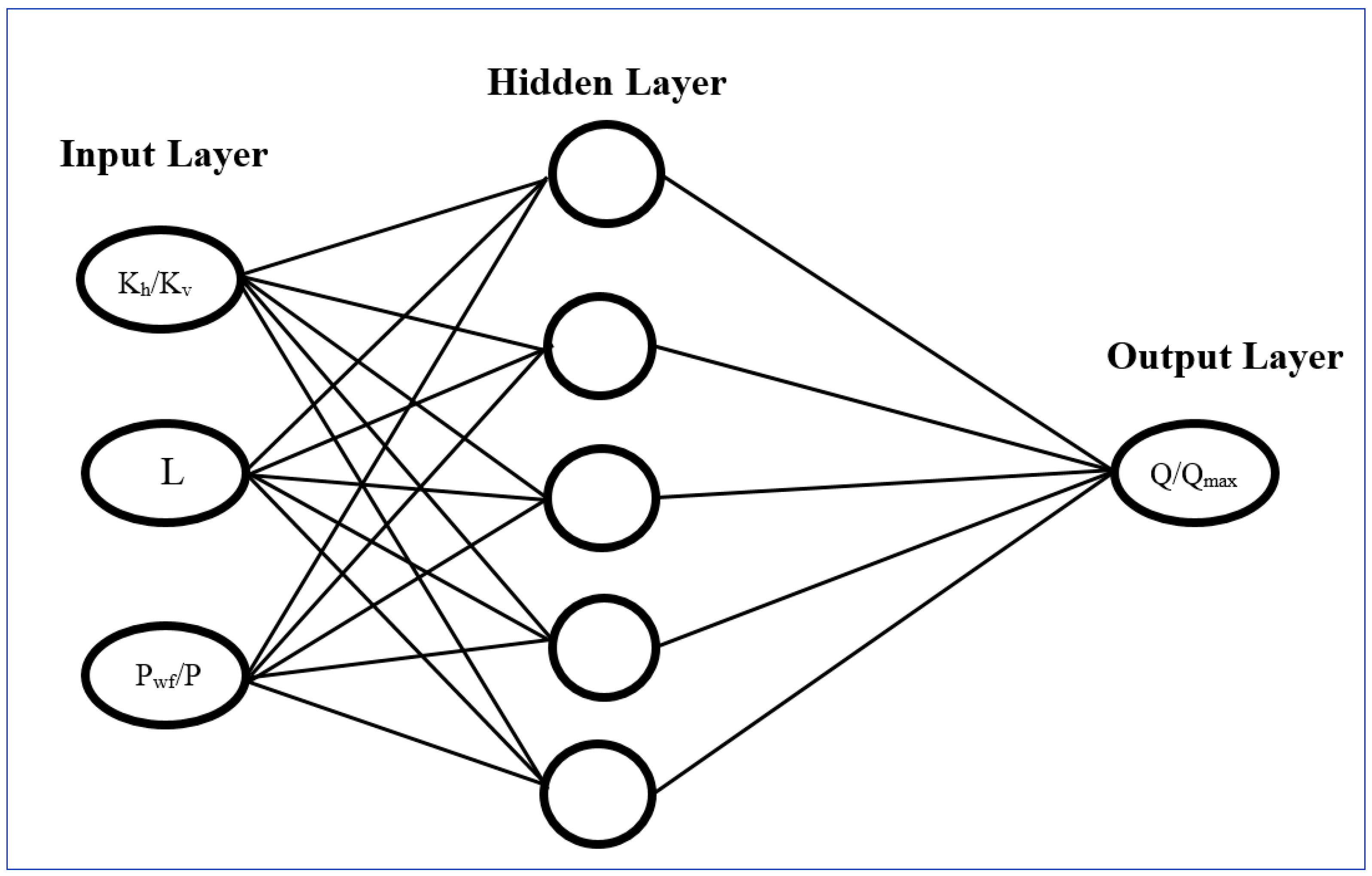
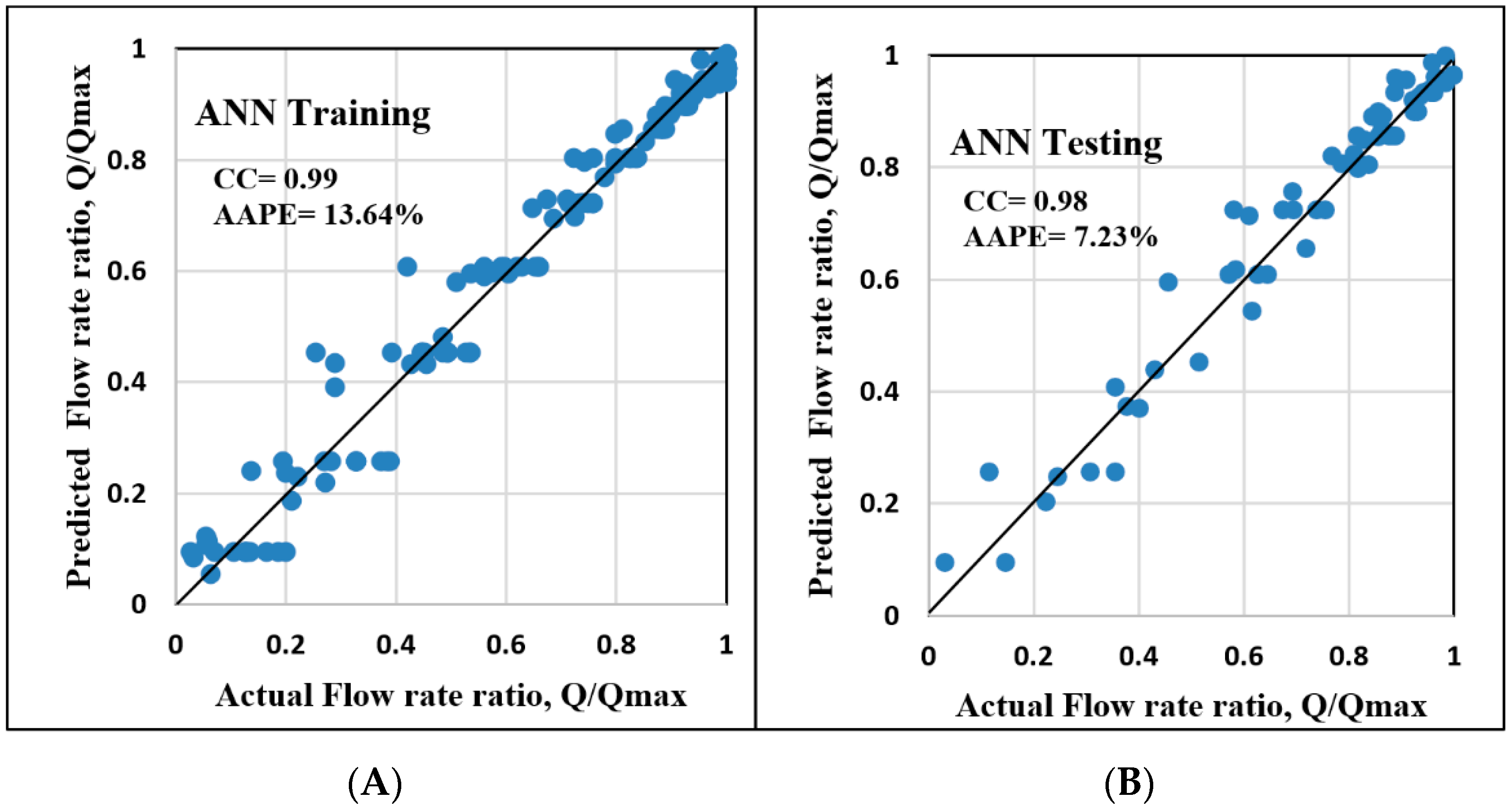
The neural network model was developed to evaluate the fishbone performance by determining the flow rate based on the well bore configurations and reservoir parameters. The model inputs were the permeability ratio, lateral length and flowing bottomhole pressure. The developed ANN model consisted of three layers: input, hidden and output. The optimum number of neurons was found to be 5 (see Figure 4). The ANN model was trained using 70% of the data, after which the model became ready to predict the flow rate for the testing or unseen data. Different cases were investigated in order to optimize the model parameters, the results of which are summarized in

Table 2. Artificial neural network results.

Case No.	No. of Hidden Layers	Number of Neurons in Layer	CorrCoef_Test	AAPE_Test
1	1	10	0.9849	15.7040
2	1	20	0.9796	7.2327
3	2	20	0.9547	14.4647
4	3	20	0.9868	11.6491

. Four cases were investigated, each with a different number of neurons (from 1 to 20 in each layer) or a different number of hidden layers (between 1 and 3). From this, optimum values for the number of neurons and layers were able to be defined. A minimum average absolute error of 7.23% and a relatively high correlation coefficient of 0.979 were obtained using 1 hidden layer with 20 neurons. Figure 5 shows the predicted results against the actual values for the training and testing data.

3.2. Fuzzy Logic System

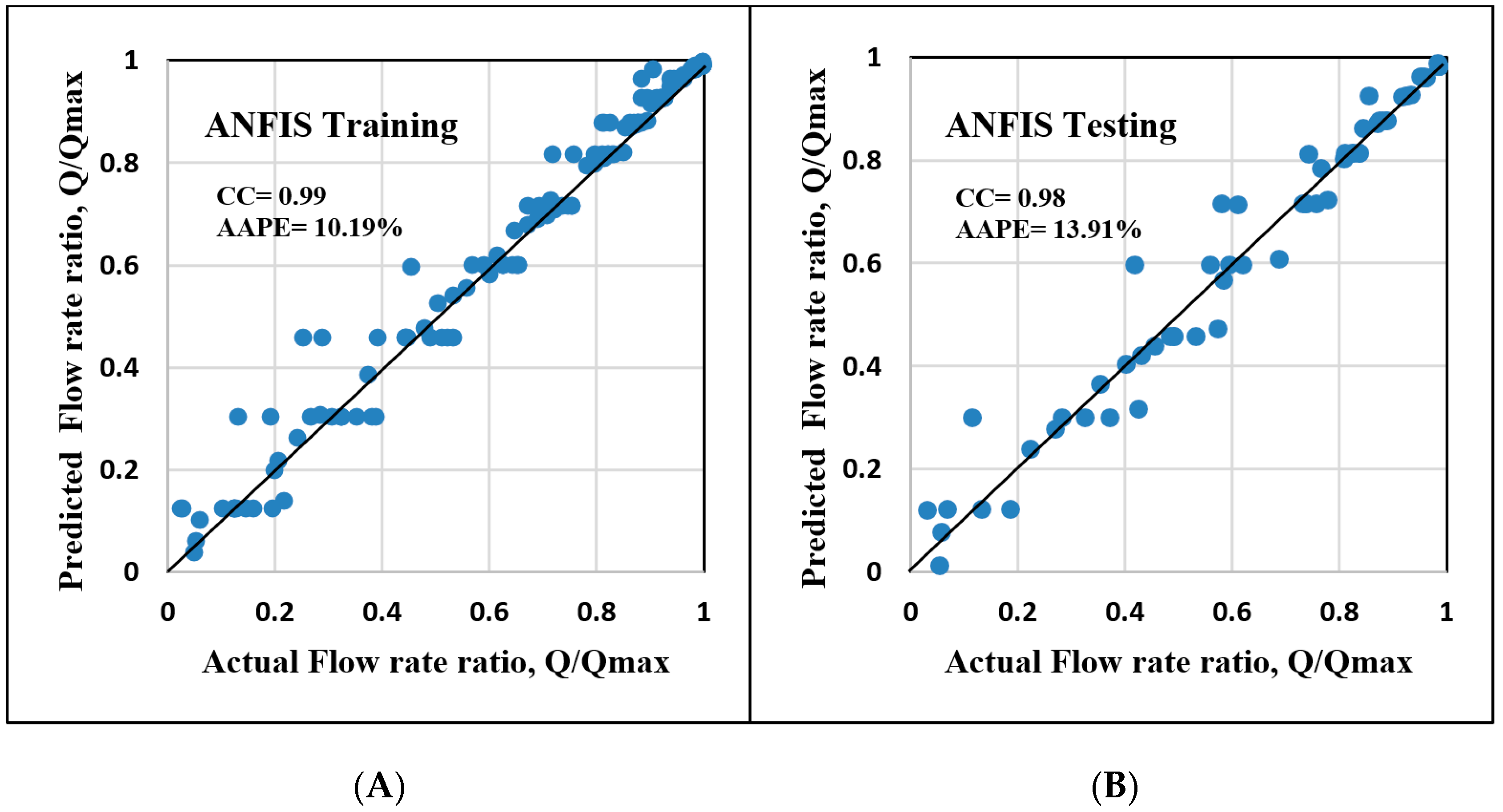
Fishbone productivity was estimated using an adaptive neuro-fuzzy inference system (ANFIS). Several scenarios were studied to fine tune the model parameters in order to minimize the estimation error and maximize the correlation coefficient, and

Table 3. Adaptive neuro-fuzzy inference system (ANFIS) results.

Case No	Cluster Radius	Number of Iterations	CorrCoef_Test	AAPE_Test
1	0.1	200	0.9822	14.4962
2	0.3	200	0.9838	14.1589
3	0.8	200	0.9845	13.9187
4	0.7	200	0.9845	13.9242
5	1	200	0.9845	13.9208
6	0.6	100	0.9848	14.0791

summarizes the ANFIS results. The optimum model was selected based on the absolute error, correlation coefficients and visualization check. Usually, better results can be obtained by increasing the cluster radius; or increasing the number of iterations. In this study, the best scenario was achieved by using five membership functions, a linear output membership function, a cluster radius of 0.8 and an iteration number of 200 (Case 3), for which the AAPE was 13.92% and the correlation coefficient was 0.985. Figure 6 shows the actual values against the predicted flow rates using the fuzzy logic model.

3.3. Radial Basis Function (RBF) Network

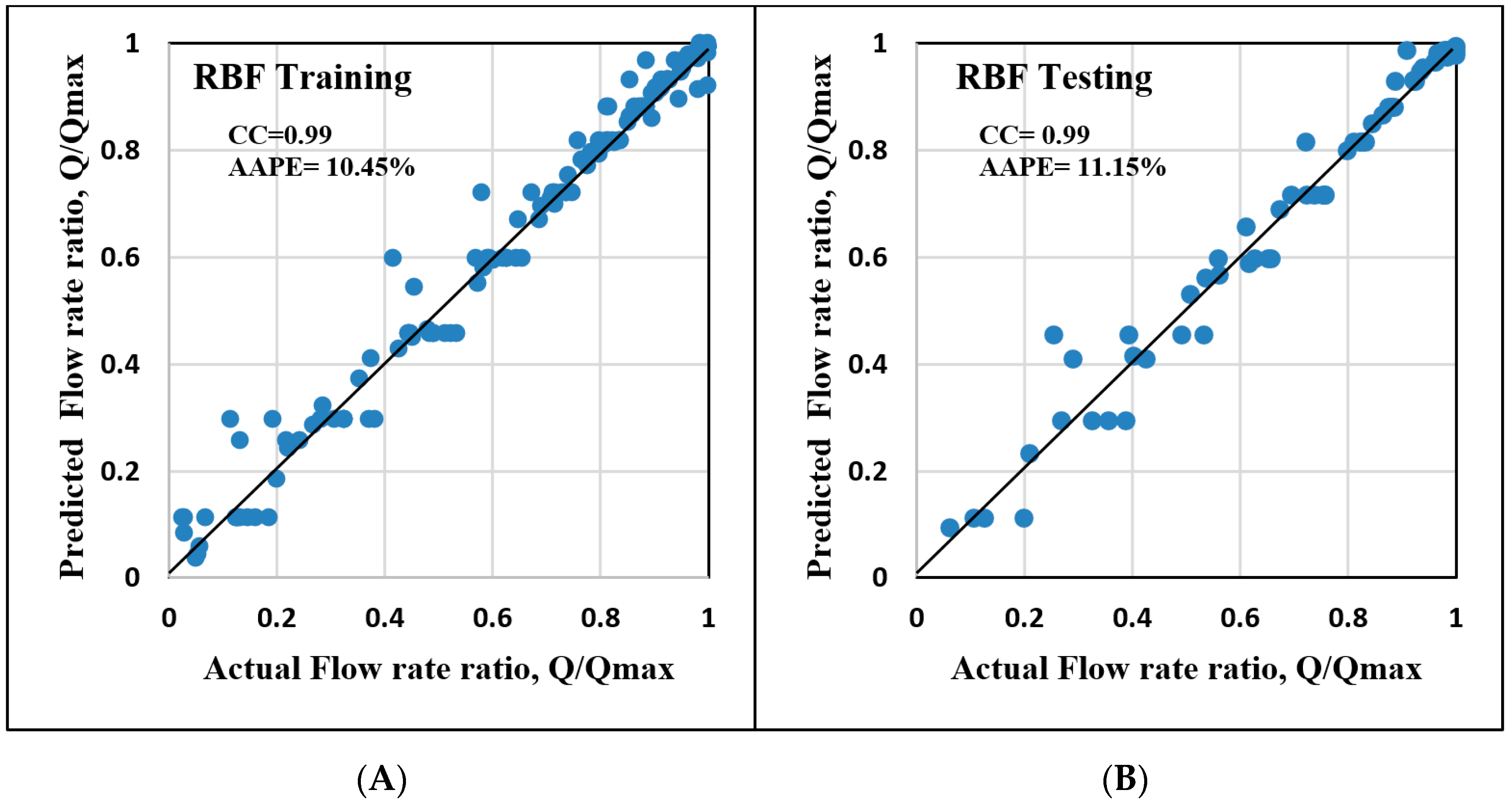
Finally, an RBF network was utilized to predict the fishbone production rate, and the impact of the model parameters on improving the model prediction was investigated. Different values of goal, spread and maximum number of neurons were examined to optimize the model parameters, with the results of this examination summarized in

Table 4. Radial basis function network (RBF) results.

Case No.	GOAL	SPREAD	MN, Maximum Number of Neurons	CorrCoef_Test	AAPE_Test
1	0	100	10	0.8786	19.3701
2	0	100	15	0.9830	11.4670
3	0	100	20	0.9851	11.1697
4	0	50	20	0.9851	11.1464
5	0.5	10	20	0.8614	32.8188

. It may be observed that increasing the goal or spread values led to worse results (higher AAPE and lower CC values), which could be due to increasing the model’s tolerance. In this work, changing the goal value showed insignificant effect in improving the prediction performance, while reducing the model’s spread led to considerable improvements in the prediction performance. Also, no further improvement was observed by increasing the maximum number of neurons (MN) above 20. The optimum case (case 4) was obtained using a goal value of 0.0, a spread value of 50, an MN of 20 and a DF (number of neurons to be added between displays) of 1. For this case, the correlation coefficient was 0.985 and the absolute error was 11.14%. Figure 7 shows the actual flow rate against the predicted flow rate using this optimal RBF model.

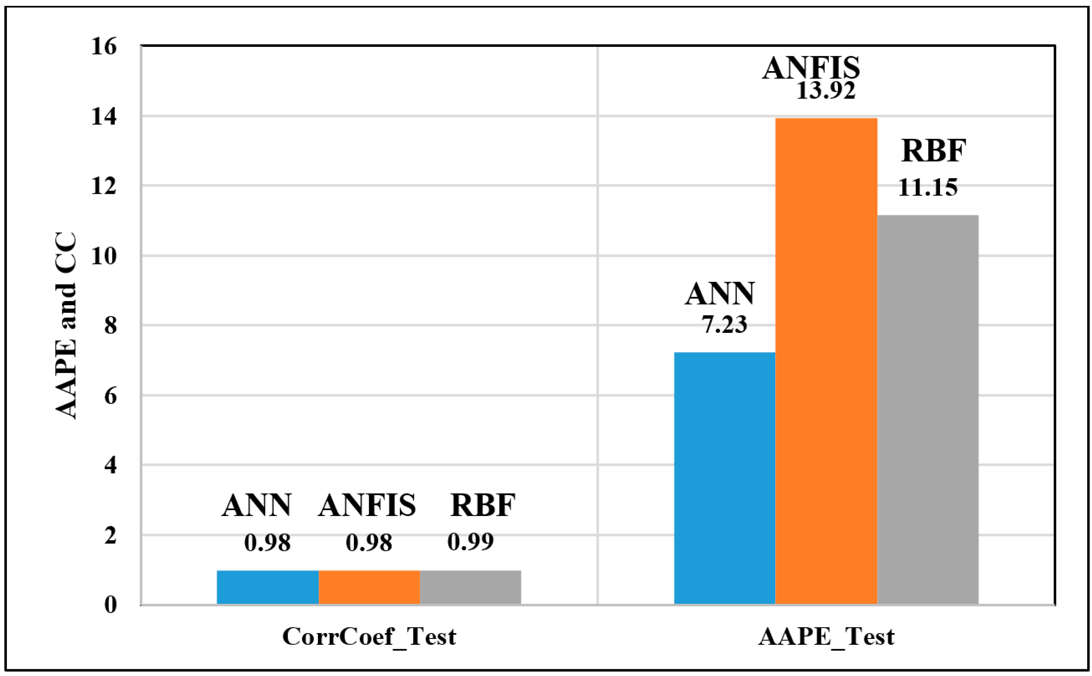
Figure 8 compares the fishbone productivity obtained using the artificial neural network (ANN), fuzzy logic system (ANFIS) and radial basis function (RBF), for which the absolute errors are 7.23%, 13.92% and 11.15%, respectively, and the correction coefficients are between 0.98 and 0.99 for all methods. The model developed using an artificial neural network showed the best prediction performance, with the absolute error of 7.23% indicating that the ANN model may be the preferred model for determining the flow rate of a fishbone well.

3.4. New Empirical Correlation for Fishbone Productivity

An empirical equation was extracted from the optimized neural network model (Equation (2)). This extracted equation can predict the flow rate based the weights and biases of the ANN model.

Table 5. The values of weights and biases extracted from the ANN model.

Neurons (N)	Weights between Input and Hidden Layer (W1)			Weights between Hidden and Output Layer (W2)	Hidden Layer Bias (b1)	Output Layer Bias (b2)
	Kh/Kv	Length	Pwf
1	−3.84692	0.617902	−2.26283	−2.819227146	0.752135	−0.28498
2	3.358502	−2.56259	−1.34471	−2.498195347	0.232057
3	3.162647	−3.3314	1.433747	−0.682675154	0.430348
4	2.595679	−3.26074	−1.83961	0.666775968	−0.9063
5	−2.19077	2.3777	1.716382	−2.423948008	0.130544
6	−1.74031	2.608322	2.778165	−0.581621184	0.281862
7	1.455491	−2.75341	−2.49005	0.699240526	−0.74851
8	−1.01596	1.755128	1.831094	−2.721731367	−0.23775
9	−0.51291	2.085212	1.655426	−2.701708506	−0.15973
10	−0.30873	3.380575	−1.66117	0.602113511	0.173508
11	0.169321	−1.10784	−3.44826	−1.33129177	0.285198
12	−0.35496	−1.95086	−2.1071	2.340221069	−0.05304
13	1.08924	2.348532	1.9611	−2.136881713	0.191233
14	1.407857	0.420195	2.554844	2.696650854	0.15787
15	−1.74964	−1.27965	−0.31507	3.224532039	−0.16893
16	−2.24378	−1.25899	1.524934	−3.236788256	−0.11517
17	−2.61158	−2.64587	−2.30505	1.377837678	−0.07059
18	3.316892	3.350453	0.264872	−1.109735463	−0.12635
19	3.298386	1.357587	−3.4066	−0.837658734	0.641118
20	3.717023	0.598516	−3.12083	1.403728747	0.227681

lists the values of weights and biases used in Equation (2). The proposed model to predict the fishbone productivity is given by the following equations:

$$\frac{\mathrm{q}}{{\mathrm{q}}_{\max }}=\left[{\displaystyle \sum }_{\mathrm{i}=1}^{\mathrm{N}}{\mathrm{w}}_{2\mathrm{i}}\tan \mathrm{sig}\left({\displaystyle \sum }_{\mathrm{j}=1}^{\mathrm{J}}{\mathrm{w}}_{1\mathrm{i},\mathrm{j}}{\mathrm{x}}_{\mathrm{j}}+{\mathrm{b}}_{1\mathrm{i}}\right)\right]+{\mathrm{b}}_2$$

(1)

$$\frac{\mathrm{q}}{{\mathrm{q}}_{\max }}=\left[{\displaystyle \sum }_{\mathrm{i}=1}^{\mathrm{N}}{\mathrm{w}}_{2\mathrm{i}}\left(\frac{2}{1+{\mathrm{e}}^{-2\left({\mathrm{w}}_{1\mathrm{i},1}{\left(\frac{{\mathrm{K}}_{\mathrm{h}}}{{\mathrm{K}}_{\mathrm{v}}}\right)}_{\mathrm{j}}+{\mathrm{w}}_{1\mathrm{i},2}{\mathrm{L}}_{\mathrm{j}}+{\mathrm{w}}_{1\mathrm{i},3}{\left({\mathrm{P}}_{\mathrm{wf}}/{\mathrm{P}}_{\mathrm{avg}}\right)}_{\mathrm{j}}+{\mathrm{b}}_{1\mathrm{i}}\right)}}\right)\right]+{\mathrm{b}}_2$$

(2)

where N is the total number of neurons, w1 is the weights of the hidden layer, w₂ is the weights of the output layer, K_h/K_v is the permeability ratio, L is the lateral length, P_wf is the flowing bottomhole pressure, and P_avg is the average reservoir pressure. Note that the ANN model automatically normalizes the input into a range between −1 and 1.

3.5. Model Verification

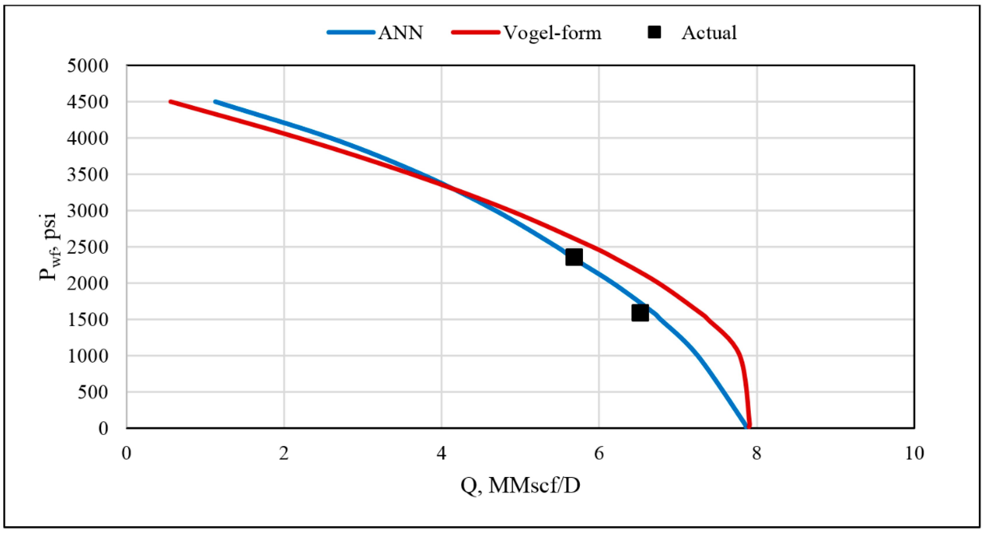
Our developed correlation was used to determine the fishbone productivity for the unseen data. More than 70 data sets with different conditions of reservoir parameters and well bore configurations were used. This correlation achieved an average absolute error of 7.23% and a relatively high correlation coefficient of 0.979. Moreover, the developed correlation was compared with different numerical and analytical models proposed in the literature. Ahmed et al. [6] proposed an empirical IPR correlation based on Vogel’s productivity model. Ahmed’s correlation (Equation (3)) can be used to determine the productivity of a fishbone well drilled into a dry gas reservoir. Based on a literature review, Ahmed’s correlation is considered one of the most accurate models that can be used to estimate the gas flow rate for fishbone wells. Therefore, the reliability of the developed ANN-based correlation was compared with that of Ahmed’s model. Figure 9 shows a comparison between the gas flow rate predicted using Ahmed’s correlation and the ANN-based correlation proposed in this work. It is clear that the flow rates predicted using the developed ANN correlation are a better match with the actual flow rate data than Ahmed’s model. Also, at low pressure, the Vogel-form equation overestimates the production rate, while the developed ANN correlation has excellent predictions. The developed empirical equation based on the optimized ANN model predicted the flow rate with an average absolute error of 6.92%.

$$\frac{q}{q_{max}}=1.00756+1.154379*{\left(\frac{P_{wf}}{P_{wfmax}}\right)}^{1.35}-2.15268*{\left(\frac{P_{wf}}{P_{wfmax}}\right)}^{1.7}$$

(3)

Overall, this work can increase the confidence of decision makers in deciding to drill more fishbone wells, instead of drilling vertical or horizontal wells. The main issue with drilling fishbone wells is that most of the available production models are inaccurate, which leads to significant deviations between the models’ results and the actual production data. As a consequence, most of the petroleum engineering industry prefer to drill vertical or horizontal wells in order to reduce the drilling cost and avoid the risk of fishbone wells, as it is easier to estimate the production rate for a vertical or horizontal well compared to a fishbone well. However, developing accurate models for determining fishbone well productivity can add to the credibility of such complex wells. The AI models presented in this paper can be used to provide an accurate estimation for the hydrocarbon production of multilateral fishbone wells, which will help in designing and optimizing production plans. Ultimately, this work can help in growing the application of complex wells, which can improve the sustainability of hydrocarbon production from underground reservoirs.

4. Conclusions

In this study, the productivity of fishbone wells was determined using three artificial intelligence techniques. The fishbone performance was estimated using a neural network model, fuzzy logic system and radial basis network. The models were developed and validated using more than 250 data sets. The following conclusions can be drawn from this work;

• The developed models showed very acceptable matches between the predicted and actual flow rates for fishbone wells.
• Only three parameters are required as inputs to the models for determining the production rate of fishbone wells: flowing bottomhole pressure, permeability ratio and lateral length.
• The developed models are able to estimate the fishbone productivity without introducing the uncertainty present in numerical models.
• The ANN model outperforms all of the artificial intelligence methods in predicting the fishbone productivity. Absolute errors of 7.23%, 13.92%, and 11.14% were obtained using the neural network, fuzzy logic and radial basis function models, respectively.
• An empirical equation was extracted from the ANN model which can provide a direct and simple determination of fishbone productivity.
• The extracted ANN-based equation can be inserted into commercial production software to provide more accurate predictions for fishbone productivity.
• The proposed models can help production engineers in designing and optimizing their production plans for complex wells.

References

- Bosworth, X.; El-Sayed, H.S.; Ismail, G.; Ohmer, H.; Stracke, M.; West, C.; Retnanto, A. Key Issues in Multilateral Technology. Oilfield Rew. 1998, 10, 14–28. [Google Scholar]
- Guangyu, X.; Guo, F.; Cheng, S.; Sun, Y.; Yu, J.; Wang, G. Fishbone Well Drilling and Completion Technology in Ultra-Thin Reservoir. In Proceedings of the IADC/SPE Asia Pacific Drilling Technology Conference and Exhibition (Paper IADC/SPE 155958), Tianjin, China, 9–11 July 2012. [Google Scholar]
- Filho, J.C.; Yifei, X.; Sepehrnoori, K. Modeling Fishbones Using the Embedded Discrete Fracture Model Formulation: Sensitivity Analysis and History Matching. In Proceedings of the SPE Annual Technical Conference and Exhibition (SPE-175124-MS), Houston, TX, USA, 28–30 September 2015. [Google Scholar]
- Guo, B.; Sun, K.; Ghalambo, A. Well Productivity Hand Book; Gulf Publishing Company: Houston, TX, USA, 2008; pp. 226–230. [Google Scholar]
- Furui, K.; Zhu, D.; Hill, A.D. A Comprehensive Model of Horizontal Well Completion Performance. In Proceedings of the SPE Annual Technical Conference and Exhibition (Paper SPE 84401), Denver, CO, USA, 5–8 October 2003. [Google Scholar]
- Ahmed, M.E.; Alnuaim, S.; Abdulazeem, A. New Algorithm to Quantify Productivity of Fishbone Type Multilateral Gas Well. In Proceedings of the SPE Annual Technical Conference and Exhibition (SPE-181888-MS), Dubai, UAE, 26–28 September 2016. [Google Scholar]
- Borisov, J.P. Oil Production Using Horizontal and Multiple Deviation Wells; Joshi, S.D., Ed.; Strauss, J., Translator; Phillips Petroleum Co.: Bartlesville, OK, USA, 1984. [Google Scholar]
- Economides, M.J.; Hill, A.D.; Economides, C. Petroleum Production Systems; Prentice Hall PTR: Upper Saddle River, NJ, USA, 1994. [Google Scholar]
- Salas, J.R.; Clifford, P.J.; Jenkins, D.P. Multilateral Well Performance. In Proceedings of the Western Regional Meeting (Paper SPE 35711), Anchorage, AK, USA, 22–24 May 1996. [Google Scholar]
- Yildiz, T. Multilateral Horizontal Well Productivity. In Proceedings of the SPE Europec/EAGE Annual Conference (Paper SPE 94223), Madrid, Spain, 13–16 June 2005. [Google Scholar]
- Xiance, Y.; Guo, B.; Ai, C.; Bu, Z. A comparison between multi-fractured horizontal and fishbone wells for development of low-permeability fields. In Proceedings of the Asia Pacific Oil and Gas Conference and Exhibition (Paper SPE 120579), Jakarta, Indonesia, 4–6 August 2009. [Google Scholar]
- Lian, P.; Cheng, L.; Tan, X.; Li, L. A model for coupling reservoir inflow and wellbore flow in fishbone wells. Pet. Sci. J. 2012, 9, 336–342. [Google Scholar] [CrossRef] [Green Version]
- Ding, Z.; Liu, Y.; Gong, Y.; Xu, N. A new technique: Fishbone well injection. Pet. Sci. Technol. 2012, 30, 2488–2493. [Google Scholar] [CrossRef]
- Freyer, R.; Shaoul, J.R. Laterals stimulation method. In Brasil Offshore Conference and Exhibition; SPE-143381-MS; Society of Petroleum Engineers: Macae, Brazil, 2011. [Google Scholar] [CrossRef]
- Abdulazeem, A.; Alnuaim, S. New Method to Estimate IPR for Fishbone Oil Multilateral Wells in Solution Gas Drive Reservoirs. In Proceedings of the SPE Kingdom of Saudi Arabia Annual Technical Symposium and Exhibition (SPE-182757-MS), Dammam, Saudi Arabia, 25–28 April 2016. [Google Scholar]
- Al-Mashhad, A.S.; Al-Arifi, S.A.; Al-Kadem, M.S.; Al-Dabbous, M.S.; Buhulaigah, A. Multilateral Wells Evaluation Utilizing Artificial Intelligence. In Proceedings of the Abu Dhabi International Petroleum Exhibition and Conference (SPE-183508-MS), Abu Dhabi, UAE, 7–10 November 2016. [Google Scholar]
- McCullock, W.S.; Pitts, W. A logical calculus of the ideas immanent in nervous activity. Bull. Math. Biophys. 1943, 5, 115–133. [Google Scholar] [CrossRef]
- Bailey, D.; Thompson, D. How to Develop Neural Network. AI Expert 1990, 5, 38–47. [Google Scholar]
- Rosenblatt, F. The Perceptron, A Perceiving and Recognizing Automaton; Project Para Report No. 85-460-1; Cornell Aeronautical Laboratory (CAL): Buffalo, NY, USA, 1957. [Google Scholar]
- Fausett, L. Fundamentals of Neural Networks, Architectures, Algorithms, and Applications; Prentice-Hall Inc.: Eaglewood Cliffs, NJ, USA, 1994. [Google Scholar]
- Ali, J.K. Neural Networks: A new Tool for the Petroleum Industry. In Proceedings of the European Petroleum Computer Conference, Aberdeen, UK, 15–17 March 1994. [Google Scholar]
- Russell, S.J.; Norvig, P. Artificial Intelligence: A Modern Approach, 3rd ed.; Prentice Hall: Upper Saddle River, NJ, USA, 2009; ISBN 0-13-604259-7. [Google Scholar]
- Sargolzaei, J.; Saghatoleslami, N.; Mosavi, S.M.; Khoshnoodi, M. Comparative Study of Artificial Neural Networks (ANN) and statistical methods for predicting the performance of Ultrafiltration Process in the Milk Industry. Iran. J. Chem. Eng. 2006, 25, 67–76. [Google Scholar]
- Lippmann, R. An introduction to computing with neural nets. IEEE ASSP Mag. 1987, 4, 4–22. [Google Scholar] [CrossRef]
- Jain, A.K.; Mao, J.; Mohiuddin, K.M. Artificial neural networks: A tutor. Computer 1996, 29, 31–44. [Google Scholar] [CrossRef]
- MathWorks, Inc. Neural Network Toolbox 6, User’s Guide. 2008. Available online: http://128.174.199.77/matlab_pdf/nnet.pdf (accessed on 30 June 2019).
- Tahmasebi, P. A hybrid neural networks-fuzzy logic-genetic algorithm for grade estimation. Comput. Geosci. 2012, 42, 18–27. [Google Scholar] [CrossRef] [PubMed] [Green Version]
- Broomhead, D.S.; David, L. Radial basis functions, multi-variable functional interpolation and adaptive networks. 1988. Available online: https://pdfs.semanticscholar.org/b08b/a914037af6d88d16e2657a65cd9dc5cf5da1.pdf (accessed on 30 June 2019).
- AlAjmi, M.D.; Alarifi, S.A.; Mahsoon, A.H. Improving Multiphase Choke Performance Prediction and Well Production Test Validation Using Artificial Intelligence: A New Milestone. In Proceedings of the SPE Digital Energy Conference and Exhibition (SPE-173394-MS), The Woodlands, TX, USA, 3–5 March 2015. [Google Scholar]
- Alarifi, S.A.; AlNuaim, S.; Abdulraheem, A. Productivity Index Prediction for Oil Horizontal Wells Using Different Artificial Intelligence Techniques. In Proceedings of the SPE Middle East Oil & Gas Show and Conference (SPE-172729-MS), Manama, Bahrain, 8–11 March 2015. [Google Scholar]
- Chen, F.; Duan, Y.; Zhang, J.; Wang, K.; Wang, W. Application of neural network and fuzzy mathematic theory in evaluating the adaptability of inflow control device in horizontal well. J. Pet. Sci. Eng. 2015, 134, 131–142. [Google Scholar]
- Elkatatny, S.; Mahmoud, M.; Tariq, Z.; Abdulraheem, A. New insights into the prediction of heterogeneous carbonate reservoir permeability from well logs using artificial intelligence network. Neural Comput. Appl. 2018, 30, 2673–2683. [Google Scholar] [CrossRef]
- Elkatatny, S.; Tariq, Z.; Mahmoud, M. Real time prediction of drilling fluid rheological properties using Artificial Neural Networks visible mathematical model (white box). J. Pet. Sci. Eng. 2016, 146, 1202–1210. [Google Scholar] [CrossRef]
- Van, S.L.; Chon, B.H. Effective Prediction and Management of a CO2 Flooding Process for Enhancing Oil Recovery using Artificial Neural Networks. ASME J. Energy Resour. Technol. 2018, 140, 032906. [Google Scholar] [CrossRef]
- Van, S.L.; Chon, B.H. Evaluating the critical performances of a CO2–Enhanced oil recovery process using artificial neural network models. J. Pet. Sci. Eng. 2017, 157, 207–222. [Google Scholar] [CrossRef]
Figure 1.
Hydrocarbon productivity for vertical, horizontal and fishbone wells.
Figure 2.
Distributions of input and output data, including (A) permeability ratio (Kh/Kv), (B) lateral length (L), (C) flowing bottomhole pressure (Pwf) and (D) flow rate.
Figure 3.
The relative importance of production rate with input parameters used to train the artificial neural network (ANN) model.
Figure 4.
Artificial neural network model architecture with input, hidden, and output layer.
Figure 5.
Comparison between the predicted and the target flow rate ratio (Q/Qmax) using the ANN model for the (A) training and (B) testing data sets.
Figure 6.
Comparison between the predicted and the target flow rate ratio (Q/Qmax) using the ANFIS model for the (A) training and (B) testing data sets.
Figure 7.
Comparison between the predicted and the target flow rate ratio (Q/Qmax) using the RBF model for the (A) training and (B) testing data sets.
Figure 8.
Comparison of different artificial intelligence (AI) techniques.
Figure 9.
Comparison between the gas flow rate predicted by the ANN model and the Vogel-form equation alongside the actual gas rate.