Quantitative Influence of Land-Use Changes and Urban Expansion Intensity on Landscape Pattern in Qingdao, China: Implications for Urban Sustainability

Abstract

The spatial structure and configuration of land-use patches, i.e., landscape patterns could affect the flow of energy and materials in inner-urban ecosystems, and hence the sustainable development of urban areas. Studying landscape pattern changes under the process of urbanization would have implicational significance to urban planning and urban sustainability. In this paper, land-use change and urban expansion intensity (UEI) were treated as the inducement factors for changes in landscape patterns, and stepwise regression and geographically weighted regression (GWR) were adapted to quantify their integrated and distributed magnitude effects on landscape patterns, respectively. The findings suggested that land-uses have different contributions to changes in landscape patterns at different urban development zones (downtown, suburban plain area and mountainous suburban areas). Furthermore, the GWR analysis results indicated that the effect of UEI on landscape patterns has spatial and temporal heterogeneity. From 1987 to 2000, the UEI had great explanatory capacity on changes in landscape patterns and helped the landscape assemble faster in the downtown and adjacent areas. However, with the shifting of the center of urban construction from downtown to the suburbs, the high explanatory ability was oriented towards suburban areas during 2000–2016 and the magnitude of influence spatially changed. Therefore, a compact city and protection policy should be adapted to different regions in the study area to achieve strong urban sustainability.

1. Introduction

The concentrations of population and socioeconomic activities in urban areas have led to fast urban expansion all around the world in recent decades [1,2]. If this aggregation phenomenon continues, land transformed into urban areas will nearly triple by the end of 2030 [3]. Meanwhile, other land-use types such as agricultural and forest land around urban areas will be embezzled during the rapid expansion of cities. These tremendous land-use changes and intensive human activities put forward serious challenges to human and natural environment [4,5], such as the loss of biodiversity [6], an increase of the urban heat island effect [7], continuous environmental degradation [8,9], decreased watershed runoff and increased flood potential in urban areas [10], and enhanced CO2 emissions [11]. Furthermore, changes in the spatial structure and configuration of land-use patches, i.e., landscape patterns, have a direct impact on urban sustainability because they determine energy flow efficiency and air pollution [12,13]. Therefore, the magnitude of influence from variations of land-use on landscape patterns determines their impact on urban sustainability. Thus, the quantitative relationship between land-use and landscape patterns is an important issue to study.

A lot of previous studies have observed land-use change and its impact on landscape patterns in rapidly urbanizing regions [1,12,14,15,16,17,18,19,20,21]. However, most of these studies have only qualitatively analyzed this relationship. For example, the conversion of agricultural land and forest land into built-up land in these areas has led to a prominent, tremendously fragmented landscape, but the magnitude of this influence has not been articulated. At the same time, the few studies using a quantitive analysis of this relationship have done so just from a perspective of their study area [15,16]. However, the effect of land-use changes on landscape patterns has been shown to vary between different urban development zones [1]. Learning the behaviors of land-use changes and the corresponding change in landscape patterns in and around urban core areas will be conductive to urban planning and urban sustainability. In this study, we analyze changes in land-use change and landscape patterns, and we describe quantitative relationships between them at different urban development zones.

Amidst land-use types, changes in built-up land is indicative of urbanization [22,23,24,25,26,27]. Urban expansion intensity, the growth rate of built-up land in an unit time interval, has been used to investigate urbanization’s impact on agricultural landscape patterns [28] and landscape patterns in land utilization [15]. However, these studies were conducted at the block and pixel levels with only several landscape metrics. However, the intensity of urbanization is more related to local government behaviors such as regional urban planning and attracting investment decisions [29]. Thus, spatial relationships between urban expansion and landscape patterns would be better conducted at the administrative division level, a comprehensive study of which could enhance the understanding of the influence of urban expansion on landscape patterns and, ultimately, benefit urban sustainable planning.

It has become easier to characterize a landscape and quantify its structural changes with advanced developments in remote sensing and geographic information science (GIS) techniques. In recent decades, a set of indices has been created to measure landscape patterns from the perspective of area, shape, aggregation and diversity [30,31,32]. In fact, these landscape indices are algorithms for quantifying specific spatial characteristics of patches, classes of patches, or entire landscape mosaics [23]. FRAGSTATS—which integrates most of the landscape indices in categories of patch, class and landscape levels—is widely used to calculate landscape metrics [33].

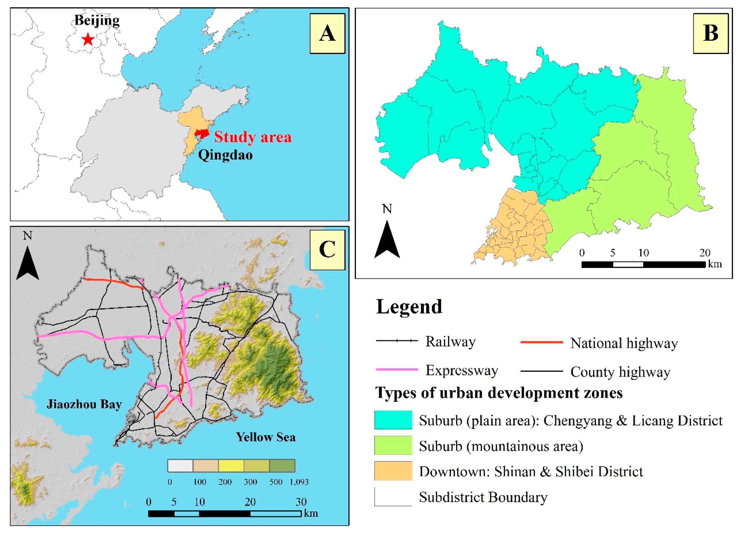
Qingdao, like most of the eastern cities of China, has experienced intensified urbanization during the last few decades [34,35]. This urban land expansion has caused great transformation in land-use and landscape patterns. Agricultural land has been converted to urban land, causing the landscape patterns to become fragmented [36]. As a result, the patch size for the remaining habitat has been reduced, and the edge effects and the isolation of patches through the destruction of connecting corridors have increased [37]. Thus, it is necessary to analyze the effect of land-use changes and urbanization on landscape pattern changes in Qingdao and to apply the results in sustainable urban planning and policymaking.

Consequently, the objectives of this study are listed as follows: (1) Identify the spatial–temporal changes of land-use and landscape patterns in three urban development zones in Qingdao; (2) quantify the effect of land-use changes on landscape pattern changes; (3) evaluate the impact of urban expansion intensity on the spatial changes of landscape patterns. Studies of these questions could provide support for urban planning and urban sustainability.

2. Materials and Methods

2.1. Study Area

Qingdao (35°35′ N–37°09′ N and 119°30′ E–121°00′ E) is in the eastern Shandong Peninsula on the east coast of China, encompassing a total land area of 1174.56 km². Surrounded by the Yellow Sea to the east and south, Qingdao has a typical maritime climate with a mean annual temperature of 12.6 °C with a cold winter (an average temperature in December–February of 0.9 °C) and mild summers (an average temperature in June–August of 23.3 °C). The mean annual precipitation is around 662 mm, and it is mostly distributed in summer (http://www.weather.com.cn/; http://www.data.ac.cn/). A natural inlet of the Yellow Sea named Jiaozhou Bay is located on the southern coast of the Shandong Peninsula. The bay is 32 km long and 27 km wide, and it has witnessed a fast development of urbanization. Qingdao City has 6 districts. We excluded Huangdao, so the other 5 districts of Shinan, Shibei, Licang, Laoshan and Chengyang were selected as the study area (Figure 1). These districts are geographically contiguous and have experienced great landscape changes during the last few decades in the process of urbanization. The terrain in this area is high in the east and low in the west, with elevation between 0 and 1133 m. Like most cities in coastal China, Qingdao has had documented high economic growth rates since 1990. Except for the global financial crisis year (2007–2008), the GDP and GDP per capita of Qingdao grew annually by double digits from 1998 to 2009 [38]. Huge economic growth resulted in great urban expansion and landscape changes in the study area. The study of these changes in response to urban sprawl could provide a clear basis for promoting the coordinated development between economics and the urban ecosystem in Qingdao.

2.2. Mapping and Analysis of Land-Use/Land Cover

Landsat images downloaded from the Geospatial Data Cloud Platform (http://www.gscloud.cn/) were used to produce the land-use/cover map of the study area. Before images were selected, two criteria were considered: (1) the date acquired must have been in the growing season (typically from around March 18 to around November 25) (https://weatherspark.com/y/136066/Average-Weather-in-Qingdao-China-Year-Round) which could be beneficial for dividing bare land and built-up land from other land types; (2) the cloud coverage had to be less than 1%. Finally, three images of Landsat 5 TM (Thematic Mapper, one sensor type) and Landsat 8 OLI (Operational Land Imager, one sensor type) acquired on 7 October 1987, 26 October 2000, and 16 June 2016 were sought out. The classification system was determined as 6 one-class level land-use types—forest land, agricultural land, built-up land, grassland, bare land and waterbody—according to previous studies and the aim of learning the influence of urbanization on agricultural and forest land [1,15,39]. During the process of classification, the images were first radiometrically calibrated and clipped with the vector boundary of the study area in the ENVI 5.3 software (Exelis Visual Information Solutions, Inc., Boulder, CO 80301 USA). Then, the spectral indices of a normalized difference vegetation index (NDVI) and normalized difference built-up index (NDBUI) [40] were calculated and stacked into multispectral bands to improve classification. Next, regions of interest (ROI), evenly distributed in the study area for both types, were delineated through visual interpretation to train and test the subsequent classification, respectively. In total, the training ROIs were 28,082, 56,484 and 45,751 pixels, and the testing ROIs were 9911, 59,464 and 36,410 pixels, respectively, for images of 1987, 2000 and 2016. Finally, the maximum likelihood classification method was used to classify images into the six land-use categories mentioned above. The overall accuracy was 92.76%, 89.66%, and 93.07% for the years of 1987, 2000 and 2016, respectively. Moreover, the Kappa coefficients were 0.90, 0.86 and 0.90, respectively, and indicated that the accuracy of land-use classification maps was high.

The conversion matrix method in ENVI was used to analyze changes in land-use/cover. The conversion matrix could provide the magnitude and intensity of changes between the different land-use types.

2.3. Analysis of Landscape Patterns

Landscape patterns have been often analyzed through landscape metrics [41]. All the metrics, which are classified into the three levels of patch, class, and landscape, quantify such aspects as the fragmentation, heterogeneity, and connectivity of the landscape pattern [21]. However, it is vital to select appropriate metrics when analyzing landscape patterns. Some methods have been used for metric selection by predecessors. For example, in order to remove surplus or redundant metrics, Schindler et al. [42] tested methods including expert knowledge, decision tree analysis, principal component analysis, and principal component regression for metric selection. On the other hand, Su et al. [39] selected metrics for an agriculture landscape pattern analysis based on the three key criteria: (1) Metrics should have some ecological significance in categories of edge/density/area, shape, and contagion; (2) metrics should be comparable with previous studies; and (3) metrics should be of low redundancy.

To comprehensively examine the urban expansion on landscape patterns, 15 frequently used landscape-level metrics [43,44,45,46] were initially selected: total area (TA), patch density (PD), the largest patch index (LPI), total edge (TE), edge density (ED), large shape index (LSI), mean shape index (SHAPE_MN), area-weighted mean shape index (SHAPE_AM), mean fractal dimension index (FRAC_MN), area-weighted fractal dimension index (FRAC_AM), contagion (CONTAG), effective mesh size (MESH), splitting index (SPLIT), Shannon’s diversity index (SHDI), and aggregation index (AI). Based on a two-tailed Pearson’s correlation analysis, 4 metrics with the least correlation between each other were chosen in this study: the LPI, SHAPE-AM, PD and CONTAG. These metrics were categorized into three groups [47]: area and edge metrics (LPI), shape metrics (SHAPE-AM), and aggregation metrics (PD and CONTAG). The area and edge metrics describe the patches’ number, size, and edge, and the shape metrics measure the geometric complexity of the patches. The aggregation metrics calculate landscape texture to describe the tendency of patch types to be spatially aggregated. All the metrics for each sub-district area were computed in FRAGSTATS 4.2 (http://www.umass.edu/landeco/research/fragstats/fragstats.html), and their change ratios were calculated based on the following Formula (1).

$$R_{\Delta t}=\frac{M_{t+\Delta t}-M_t}{M_t}\times 100\%$$

(1)

where $R_{\Delta t}$ is the change ratio of landscape metrics from time $t$ to $t+\Delta t$; $M_t$ and $M_{t+\Delta t}$ represent the value of metrics for the target unit in time $t$ and $t+\Delta t$, respectively; and $\Delta t$ is the time interval for the study period (measured in years).

2.4. Urban Expansion Intensity

In our study, the urban expansion intensity (UEI) was selected to identify urban expansion. UEI indicates the annual spatial changes of urban land area per unit area [24,25] by using Formula (2).

$$UE{I}_{\Delta t}=\frac{U{A}_{t+\Delta t}-U{A}_t}{TA}\times \frac{1}{\Delta t}\times 100\%$$

(2)

where $UE{I}_{\Delta t}$. is the urban expansion intensity during the time $t$ and $t+\Delta t$; $U{A}_t$ and $U{A}_{t+\Delta t}$ indicate the urban area of calculated unit at time $t$ and $t+\Delta t$, respectively; $\Delta t$ is the time interval of the study period (measured in years); and TA is the total land area for the target subdistrict.

2.5. Statistical and Regression Analysis

The two-tailed Pearson’s correlation method was used to analyze correlations between change in land-use and landscape metrics’ change ratio at different urban development zones and the whole study area. In addition, stepwise linear regressions were performed to quantify and compare the effects of land-use change (a unit of km² was designated) on landscape pattern changes. To evaluate the explanatory ability of models, the adjusted R² value was calculated for each model. All analyses were performed using IBM SPSS Statistics version 22 software (SPSS Inc., Chicago, IL, USA).

To assess the spatial influence of urban expansion on landscape pattern changes, geographically weighted regression (GWR) was applied to explore the relationship between urban expansion intensity and landscape metrics. Under the assumption that nearer observations exert more significant influences, GWR can accurately describe a spatial relationship by taking neighbor effects into consideration [48]. It expresses the spatial relationships of a variable by generating a group of local coefficients containing a local R² value, local residuals, local parameter estimates, and t-test values. The formulation of the GWR model can be expressed as Formula (3).

$$y_j={\beta }_0\left(u_j,v_j\right)+{\displaystyle \sum }_i^k{\beta }_i\left(u_j,v_j\right)x_{ij}+{\epsilon }_j$$

(3)

where $u_j$ and $v_j$ indicate the spatial coordinates of location j; ${\beta }_0\left(u_j,v_j\right)$ and ${\beta }_i\left(u_j,v_j\right)$ are the intercept value and the local-specific coefficient of the independent variable $x_{ij}$, respectively; k is the number of independent variable; and ${\epsilon }_j$ represents the error. GWR uses kernel bandwidth to calculate the spatial dependency range, and the weight for all observations are computed by a distance–decay function within the spatial range. This distance decay function is given as Formula (4).

$$w_{ij}=\exp \left(-d_{ij}^2/b^2\right)$$

(4)

where $w_{ij}$ represents the weight of observation i relative to neighborhood observation j; $d_{ij}$ is the Euclidean distance between locations i and j; and b represents the kernel bandwidth. Coarser kernel bandwidth leads to a slowed weight decrease with distance and generates more global relationships [49]. The weight value equals 1 when the observation points i and j are located at the same place; conversely, the weight value decay is close to 0 when the distance between them increases toward the spatial scope of kernel bandwidth.

The spatial regression model was performed with the GWR tool in the ArcGIS 10.3 software (Environmental Systems Research Institute, Redlands, CA, USA). The spatial map for the changes of each of the metrics during a time interval was taken as a dependent variable and the corresponding urban expansion intensity change was entered as an independent factor. There are two types of kernel function in the spatial regression tool: FIXED and ADAPTIVE. This means that the spatial context (the Gaussian kernel) can be a fixed distance or a function of a specified number of neighbors. In this study, the basic unit for the GWR modeling are sub-districts whose boundary and the area were irregular and unequal, i.e., the spatial distribution of observations was not uniform. Therefore, we adapted the ADAPTIVE type of kernel matched up with the lowest Akaike information criteria (AICc) to determine the extent of the kernel.

3. Results

3.1. Changes in Land-Use/Cover

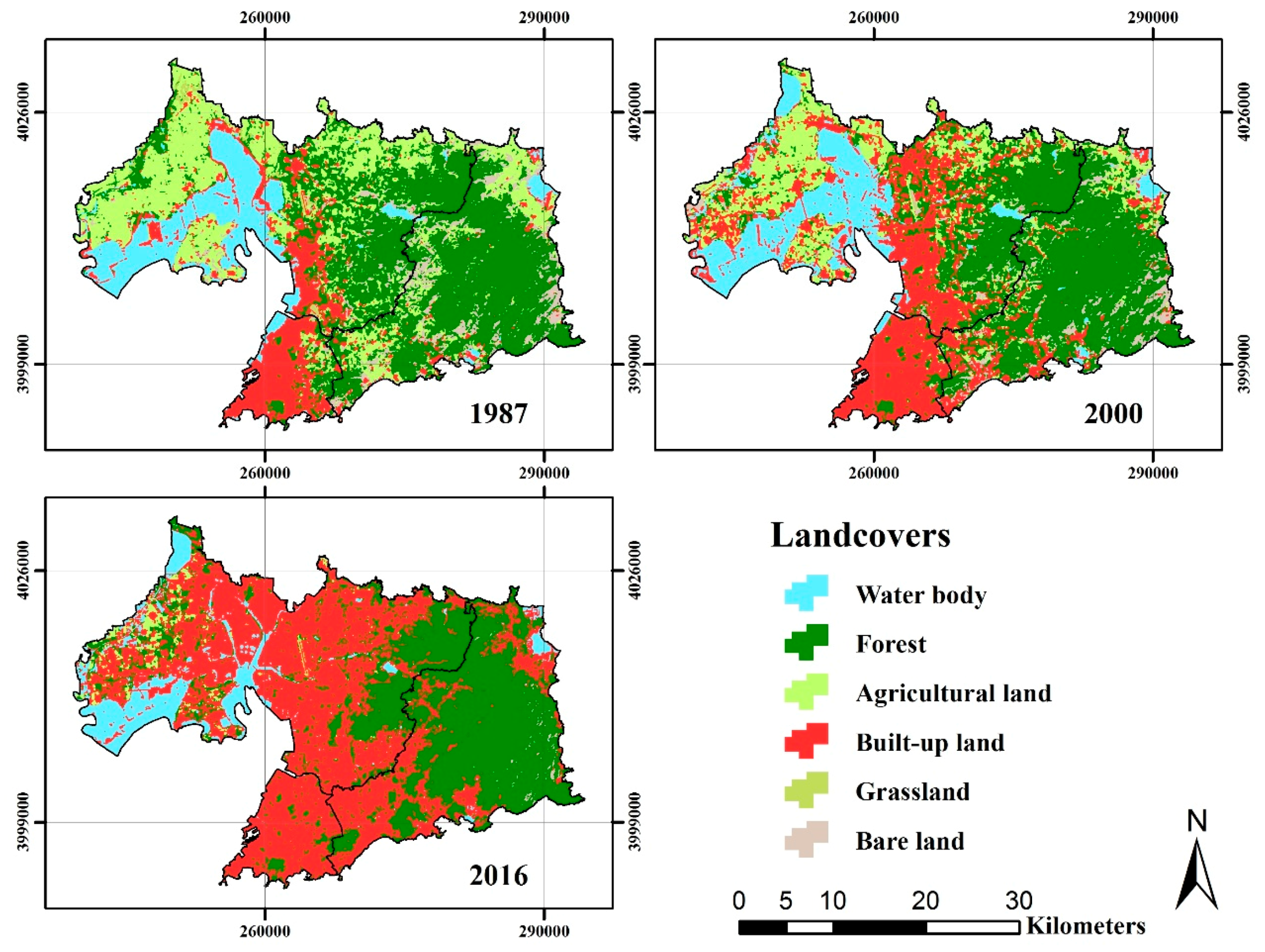
The land-use changes during the years 1987 and 2016 were examined by using spatial maps (Figure 2) and a conversion matrix (Appendix A,

Table A1. Land-use/cover conversion matrix for the whole region during the period 1987–2016 (in ha).

	1987
		Forest	Agricultural	Built-Up	Grassland	Bare Land	Water	Class Total
2000	Forest	36460.8	5893.11	658.71	923.76	1609.38	117.09	45662.85
	Agricultural	1863.63	13950.63	241.65	459.18	980.91	35.1	17531.1
	Built-up	6160.32	6967.98	12318.57	463.95	1464.39	1744.74	29119.95
	Grassland	172.26	64.8	5.49	29.16	135.72	0.09	407.52
	Bare land	1290.6	872.82	148.95	49.05	2486.79	21.42	4869.63
	Water	920.16	656.46	1330.38	322.02	64.71	11990.61	15284.34
	Class Total	46867.77	28405.8	14703.75	2247.12	6741.9	13909.05
	Image Difference	–1204.92	–10874.7	14416.2	–1839.6	–1872.27	1375.29
	Image Difference (%)	–2.57	–38.28	98.04	–81.86	–27.77	9.89
	2000
2016	Forest	33714.99	4623.57	1713.33	216.63	2659.50	509.04	43437.06
	Agricultural	248.58	1783.71	194.85	7.38	132.30	101.25	2468.07
	Built-up	11375.28	10918.53	25729.83	164.79	1762.38	6804.18	56754.99
	Grassland	11.07	50.13	10.62	18.63	9.99	6.30	106.74
	Bare land	25.83	11.97	31.05	0.09	233.19	1.89	304.02
	Water	287.10	143.19	1440.27	0.00	72.27	7861.68	9804.51
	Class Total	45662.85	17531.1	29119.95	407.52	4869.63	15284.34
	Image Difference	–2225.79	–15063.03	27635.04	–300.78	–4565.61	–5479.83
	Image Difference (%)	–4.87	–85.92	94.90	–73.81	–93.76	–35.85

,

Table A2. Land-use/cover conversion matrix for the downtown area during the period 1987–2016 (in ha).

	1987
		Waterbody	Forest	Agricultural	Built-Up	Grassland	Bare Land	Class Total
2000	Waterbody	190.71	4.14	0	1.08	3.06	0	198.99
	Forest	22.32	812.7	56.52	159.75	49.32	11.97	1112.58
	Agricultural	4.68	19.89	29.7	10.98	13.68	4.59	83.52
	Built-up	305.91	954.72	333.9	5997.24	138.06	213.57	7943.4
	Grassland	0	3.33	0.09	0	0	0	3.42
	Bare land	3.6	13.5	6.93	7.92	3.69	16.92	52.56
	Class Total	527.22	1808.28	427.14	6176.97	207.81	247.05
	Image Difference	–328.23	–695.7	–343.62	1766.43	–204.39	–194.49
	Image Difference (%)	–62.26	–38.47	–80.45	28.60	–98.35	–78.72
	2000
2016	Waterbody	3.42	8.91	0.09	9.99	0	0.09	22.50
	Forest	19.80	753.12	7.02	301.41	1.80	11.70	1094.85
	Agricultural	0	0.45	0	1.35	0	0	2.00
	Built-up	175.77	350.10	76.41	7630.65	1.62	40.77	8275.32
	Grassland	0	0	0	0	0	0	0
	Bare land	0	0	0	0	0	0	0
	Class Total	198.99	1112.58	83.52	7943.4	3.42	52.56
	Image Difference	–176.49	–17.73	–81.52	331.92	–3.42	–52.56
	Image Difference (%)	–88.69	–1.59	–97.61	4.18	–100	–100

,

Table A3. Land-use/cover conversion matrix for the suburb (plain area) during the period 1987–2016 (in ha).

	1987
		Waterbody	Forest	Agricultural	Built-Up	Grassland	Bare Land	Class Total
2000	Waterbody	11104.83	855.63	629.37	1257.75	318.33	34.38	14200.29
	Forest	77.94	13770.72	3206.34	276.3	497.61	342.09	18171.00
	Agricultural	22.23	1488.78	11903.85	159.75	406.62	360.36	14341.59
	Built-up	1355.76	4063.86	5361.84	5208.03	289.35	620.46	16899.3
	Grassland	0	56.07	32.04	5.49	29.07	66.78	189.45
	Bare land	8.28	280.71	416.34	80.64	30.87	278.64	1095.48
	Class Total	12569.04	20515.77	21549.78	6987.96	1571.85	1702.71
	Image Difference	1631.25	–2344.77	–7208.19	9911.34	–1382.4	–607.23
	Image Difference (%)	12.98	–11.43	–33.45	141.83	–87.95	–35.66
	2000
2016	Waterbody	7325.91	270.36	140.31	1329.39	0.00	70.83	9136.80
	Forest	467.82	10234.71	3335.22	1041.66	74.70	315.54	15469.65
	Agricultural	101.16	236.16	1776.69	189.18	7.29	103.32	2413.80
	Built-up	6299.10	7418.43	9037.62	14326.83	88.47	595.71	37766.16
	Grassland	6.30	11.07	50.13	10.62	18.99	9.99	107.10
	Bare land	0.00	0.27	1.62	1.62	0.00	0.09	3.60
	Class Total	14200.29	18171.00	14341.59	16899.3	189.45	1095.48
	Image Difference	–5063.49	–2701.35	–11927.79	20866.86	–82.35	–1091.88
	Image Difference (%)	–35.66	–14.87	–83.17	123.48	–43.47	–99.67

and

Table A4. Land-use/cover conversion matrix for the suburb (mountainous area) during the period 1987–2016 (in ha).

	1987
		Waterbody	Forest	Agricultural	Built-Up	Grassland	Bare Land	Class Total
2000	Waterbody	679.23	59.67	27.09	69.93	0.18	30.15	866.25
	Forest	16.74	21812.76	2621.52	221.85	372.69	1252.35	26297.91
	Agricultural	8.19	352.44	1972.44	70.92	37.26	613.71	3054.96
	Built-up	79.38	1138.14	1271.07	1101.60	34.38	630.27	4254.84
	Grassland	0.09	112.86	32.67	0	0.09	67.95	213.66
	Bare land	9.45	992.79	447.93	60.48	14.49	2186.28	3711.42
	Class Total	793.08	24468.66	6372.72	1524.78	459.09	4780.71
	Image Difference	73.17	1829.25	–3317.76	2730.06	–245.43	–1069.29
	Image Difference (%)	9.23	7.48	–52.06	179.05	–53.46	–22.37
	2000
2016	Waterbody	517.68	5.04	2.79	93.42	0	0.90	619.83
	Forest	20.70	22669.65	1273.86	369.81	139.41	2327.94	26801.37
	Agricultural	0.09	11.79	7.56	4.32	0.09	28.98	52.83
	Built-up	325.89	3585.87	1760.40	3757.86	74.07	1118.79	10622.88
	Grassland	0	0	0	0	0	0	0
	Bare land	1.89	25.56	10.35	29.43	0.09	234.81	302.13
	Class Total	866.25	26297.91	3054.96	4254.84	213.66	3711.42
	Image Difference	–246.42	503.46	–3002.13	6368.04	–213.66	–3409.29
	Image Difference (%)	–28.45	1.91	–98.27	149.67	–100	–91.86

). The results showed that urbanization has led to significant land-use changes over the years 1987–2016. Therefore, the most obvious changes occurred in built-up land, with 14,416.2 ha (growth rate of 98.04%) and 27,635.04 ha (growth rate of 94.90%) increases in the periods of 1987–2000 and 2000–2016, respectively. As a result, the proportion of built-up land in the total land has increased from 13.03% to 50.28%. This rapid urbanization process has mainly occurred around the Jiaozhou Bay, which occupies a flat terrain area near the sea. With the dramatic upsurge in built-up land, other land-use types such as forest land, agricultural land and waterbodies have been bulldozed. For example, the forest land, agricultural land and waterbody had 6160.32, 6967.98, and 1744.74 ha converted to built-up land during 1987–2000, which account for 59.19%, 48.20% and 90.95% in the changed area of the three types, respectively. This trend was more pronounced from 2000 to 2016, with the above-mentioned proportion reached 95.21%, 69.33% and 91.67%, respectively. At the same time, the built-up land had transformed into other land-use types such as waterbody and forest land during this period. This could be due to river regulation, reservoir building, and old villages’ reconstruction, all of which would generate urban green space.

Land-use changes exhibited distinct variations among different urban development zones. In the downtown area, the built-up land continuously increased from 6176.97 to 8275.32 ha during the years 1987–2016, which is 88.09% of the total downtown area. Among the augmenter in built-up land, the forest land had the largest contribution, with 49.06% land transformed during the period of 1987–2000 and 54.31% land converted from 2000 to 2016. The sea reclamation in the east of downtown is the most important inducement of the decrease of waterbody, whose area declined 62.26% and 88.69% in the periods of 1987–2000 and 2000–2016, respectively. At the same time, the other three land-use types experienced dramatic decreases because of urbanization progress. The grassland and bare land had disappeared, and the agricultural land almost vanished in 2016. However, there were also 159.75 and 301.41 ha of built-up land transformed into forest land during 1987–2000 and 2000–2016, respectively. This may benefit from the restoration and conservation of several big parks (e.g., Zhongshan Park, Beiling Mountain Forest Park, Jiading Mountain Park, Guanxiang Mountain Park and Shuangshan Park) and the construction of the coastal green belt.

In the suburban plain area, the built-up land area grew 141.83% and 123.48% during the years of 1987–2000 and 2000–2016, respectively, indicating an extreme urban expansion in this region. The increase in built-up land area was stronger across the transportation network around the Jiaozhou Bay. In other land-use types, the agricultural land had the greatest decline, with 7208.19 ha (33.45%) and 11,927.79 ha (83.17%) decreases in the periods of 1987–2000 and 2000–2016, respectively. Among the decrement, 74.39% and 75.77% of agricultural land, respectively, in the periods of 1987–2000 and 2000–2016 were converted to built-up land. Similarly, a large amount of forest land, grassland and bare land were transformed into urban land, resulting in continuous declinations for these types. On the contrary, during the years 1987–2000, the waterbody area increased 1631.25 ha, with the growth rate being 12.98%. This increase was mainly due to the construction of Jihongtan Reservoir in the north of this region. However, this trend turned in the opposite direction, with 35.66% (5063.49 ha) of the waterbody transformed into other land-use types—mainly built-up land.

In the mountainous suburban areas, the increase of built-up land in southwestern and northeastern Laoshan district reached 4254.84 ha (during 1987 and 2000) and 10,622.88 ha (during 2000 and 2016), which is 11.08% and 27.66% of the total area. At the same time, the forest land area increased 2332.71 ha from 1987 to 2016 under the influence of the Grain for Green Project and forest conservation policy in this region. In contrast, the agricultural land and bare land areas significantly declined 99.17% and 93.68%, respectively, in the years of 1987–2016, whereas the grassland completely vanished by the end of 2016. The waterbody area increased 73.17 ha from 1987 to 2016, but a great decrease of 246.42 ha followed because of the encroachment of urban land.

3.2. Spatial and Temporal Change of Landscape Patterns

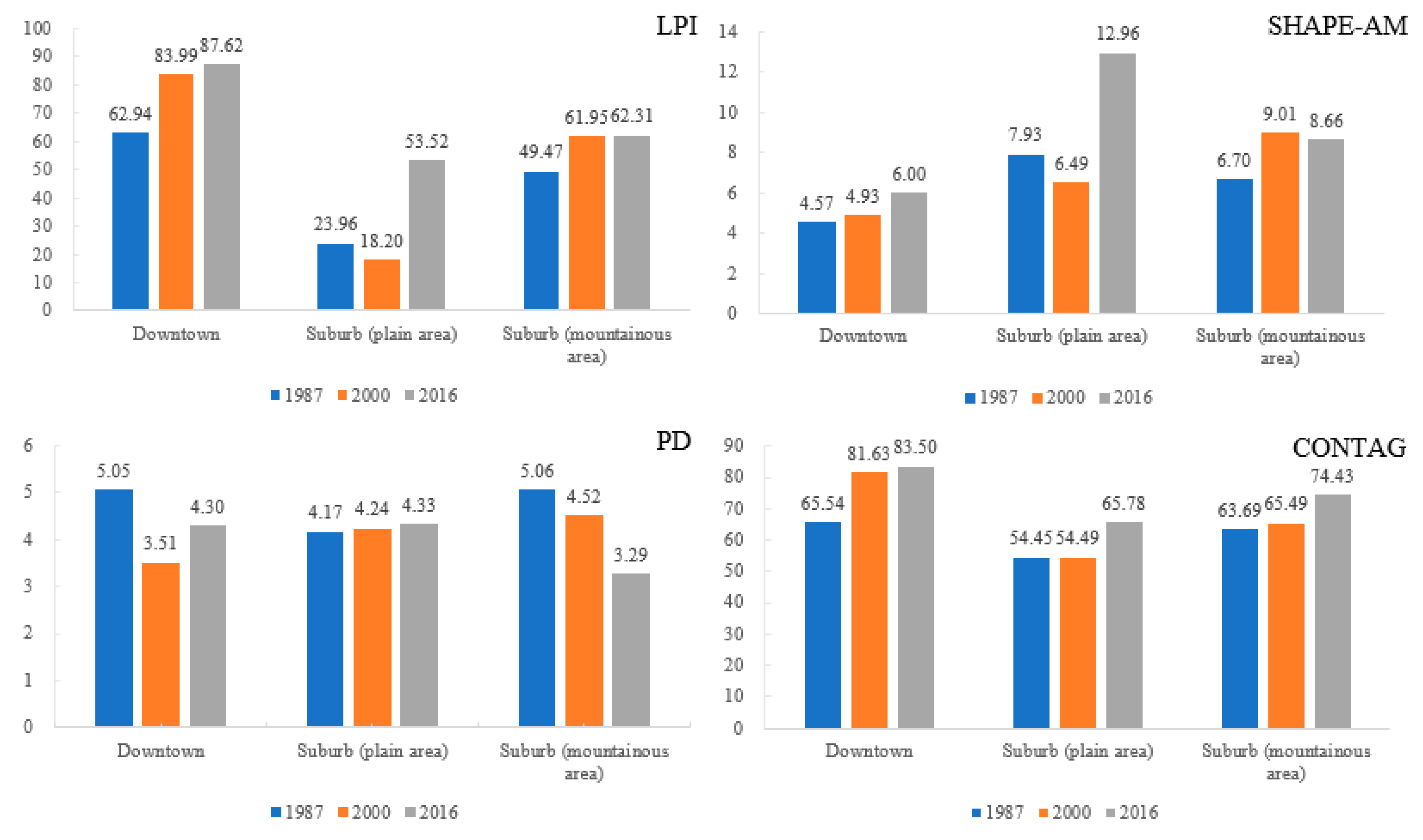
The landscape patterns of different urban development zones in the study area were analyzed through four landscape metrics during the periods of 1987, 2000 and 2016. As shown in Figure 3, the changes were obviously different across different zones for the metrics: (1) The LPI significantly increased in the downtown and mountainous suburban areas, but it decreased in the suburban plain area from 1987 to 2000. However, the LPI had a huge increase in the suburban plain area when it slightly increased in the downtown and mountainous suburban areas. The significant increase of the LPI in the downtown and mountainous suburban areas was due to the expansion and infilling of built-up land and forest land, respectively (Figure 2). As a result, the largest patch of area increased. The changes of the LPI in the suburban plain area was because the largest patch of agricultural land decreased and was finally replaced by a large patch of built-up land. (2) The area-weighted mean shape index (SHAPE-AM) continually increased in the downtown area, whereas it firstly decreased and then enormously increased in the suburban plain area and exhibited a first increasing and then decreasing tendency in the mountainous suburban areas. (3) The urbanization transformed other land-use types into built-up land and promoted the appearance of green space in the downtown area. As a result, PD significantly decreased in the period of 1987–2000 and increased in the period of 2000–2016. However, there had been consistent, slight growth and a sustained, great decrease in the suburban plain and mountainous areas, respectively. The conversion of a large patch of agricultural land and waterbody into dispersed built-up land in the suburban area, and the infilling of forest land by disappeared bare land in the mountainous suburban areas was responsible for these changes. (4) CONTAG significantly increased in downtown and slightly increased in the other two places from 1987 to 2000. However, during 2000–2016, it increased a lot in suburban plain and mountainous areas but had a slight increase in downtown.

3.3. The Influence of Land-Use Change and UEI on Landscape Patterns

A correlation analysis was conducted to identify the relationships between selected landscape metrics and land-use changes and UEI (

Table 1. Pearson’s correlation coefficients between landscape metrics changes and urbanization related to land-use changes and urban expansion intensity in different urban development zones and the whole region from 1987 to 2000.

Urban Development Zones	Landscape Metrics	Waterbody	Forest	Agricultural Land	Built-up Land	Grassland	Bare Land	UEI
Downtown area	LPI	–0.069	–0.673 **	–0.705 **	0.797 **	–0.532 **	–0.776 **
	SHAPE–AM	–0.073	0.039	–0.416 *	0.281	–0.377 *	–0.440 *
	PD	–0.182	0.637 **	0.551 **	–0.602 **	0.567 **	0.566 **
	CONTAG	–0.018	–0.595 **	–0.638 **	0.684 **	–0.563 **	–0.554 **
Suburb (mountainous area)	SHAPE-AM	0.802	–0.750	0.143	0.415	–0.974 *	0.319
The whole region	LPI	–0.124	–0.027	0.206	–0.126	0.071	–0.037	0.696 **
	SHAPE-AM	–0.067	0.067	0.023	0.025	–0.080	–0.147	0.068
	PD	0.057	0.119	–0.240	0.161	–0.079	–0.050	–0.691 **
	CONTAG	–0.081	–0.087	0.220	–0.127	0.045	–0.008	0.756 **

The superscripts ** and * indicate a significantly correlation at the 0.01 level (two-tailed) and the 0.05 level (two-tailed), respectively. LPI: largest patch index; SHAPE-AM: area-weighted mean shape index; PD: patch density; CONTAG: contagion; UEI: urban expansion intensity.

and

Table 2. Pearson’s correlation coefficients between landscape metrics changes and urbanization related to land-use changes and urban expansion intensity in different urban development zones and the whole region from 2000 to 2016.

Urban Development Zones	Landscape Metrics	Waterbody	Forest	Agricultural Land	Built-up Land	Grassland	Bare Land	UEI
Downtown area	LPI	−0.391 *	−0.724 **	–0.706 **	0.853 **	−0.463 **	–0.149
	SHAPE-AM	−0.023	0.695 **	0.304	−0.413 *	0.228	–0.192
	PD	0.103	0.376 *	0.493 **	−0.407 *	0.354 *	0.141
	CONTAG	−0.268	−0.193	−0.255	0.315	−0.098	0.316
Suburb (plain area)	SHAPE-AM	−0.299	0.367	−0.582 **	0.388	0.309	0.013
	PD	−0.308	0.642 **	−0.267	0.063	0.378	0.332
The whole region	LPI	−0.341 *	−0.013	−0.343 **	0.392 **	0.108	−0.123	0.630 **
	SHAPE-AM	−0.291 *	0.429 **	−0.639 **	0.404 **	0.081	−0.240	0.319 *
	PD	−0.061	0.307 *	0.060	−0.214	0.323 *	0.246	−0.489 **
	CONTAG	−0.191	−0.154	−0.246	0.367 **	−0.150	−0.251	0.511 **

The superscripts ** and * indicate a significantly correlation at the 0.01 level (two-tailed) and the 0.05 level (two-tailed), respectively. LPI: largest patch index; SHAPE-AM: area-weighted mean shape index; PD: patch density; CONTAG: contagion; UEI: urban expansion intensity.

). The results indicate that there have been great variations across three urban development zones and the whole study area at different time stages. From the perspective of the whole region, none of four metrics were related with land-use changes during 1987–2000. However, in the last period, the LPI was sensitive to waterbody, agricultural and built-up land; SHAPE-AM was not significantly related to grassland and bare land; PD was well-related with forest land and grassland; and CONTAG was only sensitive to built-up land. In terms of UEI, it was strongly related to all the landscape metrics in the two periods other than SHAPE-AM from 1987 to 2000.

In the downtown area, the area-edge metrics (LPI) and aggregation metrics (PD, CONTAG) were significantly related to all the land-use types except waterbody during the period of 1987–2000, whereas CONTAG was no longer significantly related to any land-use types, and the LPI and CONTAG were not sensitive to bare land during the period of 2000–2016. The shape metric (SHAPE-AM) related well to agricultural, grassland and bare land from 1987 to 2000, and it was correlated well with forest and built-up land in 2000 and 2016, respectively. In the suburban plain area, only the metrics of SHAPE-AM and PD were strongly related to forest and agricultural land during the stage of 2000–2016. In the mountainous suburban areas, only SHAPE-AM had a significant relationship with the land use of grassland from 1987 to 2000.

A stepwise regression model was used to assess which land-use was more important to the change of landscape patterns across different types of urban development zones (

Table 3. Stepwise regression models of land-use changes during 1987–2000 and the related landscape metrics in different urban development zones. The regression equations were selected because the probabilities of their F values were less than 0.05.

Urban Development Zones	Dependent Variables	Final Model	Adjusted R2	p Value
Downtown area	LPI	LPI = 1.925 + 22.801 built-up land + 89.567 grassland – 69.838 bare land	0.718	0.000
	SHAPE-AM	SHAPE-AM = -0.004 – 2.359 bare land + 0.504 forest land	0.285	0.002
	PD	PD = -0.852 + 6.439 forest land	0.387	0.000
	CONTAG	CONTAG = 0.010 + 0.220 built-up land	0.451	0.000
Suburb (mountainous area)	SHAPE-AM	SHAPE-AM = -0.179 – 1.195 grassland	0.922	0.026

LPI: largest patch index; SHAPE-AM: area-weighted mean shape index; PD: patch density; CONTAG: contagion; UEI: urban expansion intensity.

and

Table 4. Stepwise regression models of land-use changes during 2000–2016 and the related landscape metrics in different urban development zones. The regression equations were selected because of the probabilities of their F values were less than 0.05.

	Dependent Variables	Final Model	Adjusted R2	p Value
Downtown area	LPI	LPI = -0.783 + 24.866 built-up land + 13.121 waterbody – 25.781 agricultural	0.871	0.000
	SHAPE-AM	SHAPE-AM = 0.138+ 0.784 forest land	0.466	0.000
	PD	PD = 1.474 + 18.293 agricultural	0.219	0.004
Suburb (plain area)	SHAPE-AM	SHAPE-AM = 0.290 – 0.047 agricultural	0.299	0.009
	PD	PD = 0.156 + 0.214 forest land	0.377	0.003

LPI: largest patch index; SHAPE-AM: area-weighted mean shape index; PD: patch density; UEI: urban expansion intensity.

). During the period of 1987–2000, the changes of built-up land, grassland, waterbody and bare land played a significant role in predicting the LPI and CONTAG, and forest land and bare land were more important in the prediction of SHAPE-AM and PD in the downtown area. However, grass land was the only land-use type that could effectively predict SHAPE-AM in the mountainous suburban areas. Furthermore, in the period of 2000–2016, built-up land, waterbody and agricultural land played an important role in predicting the LPI in downtown, forest and agricultural land were more important to SHAPE-AM and PD in the downtown and suburban plain areas. These results indicated that the influence of land-use changes on landscape patterns was significantly different across three urban development zones.

3.4. Spatial Relationships between Urban Expansion Intensity and Landscape Patterns

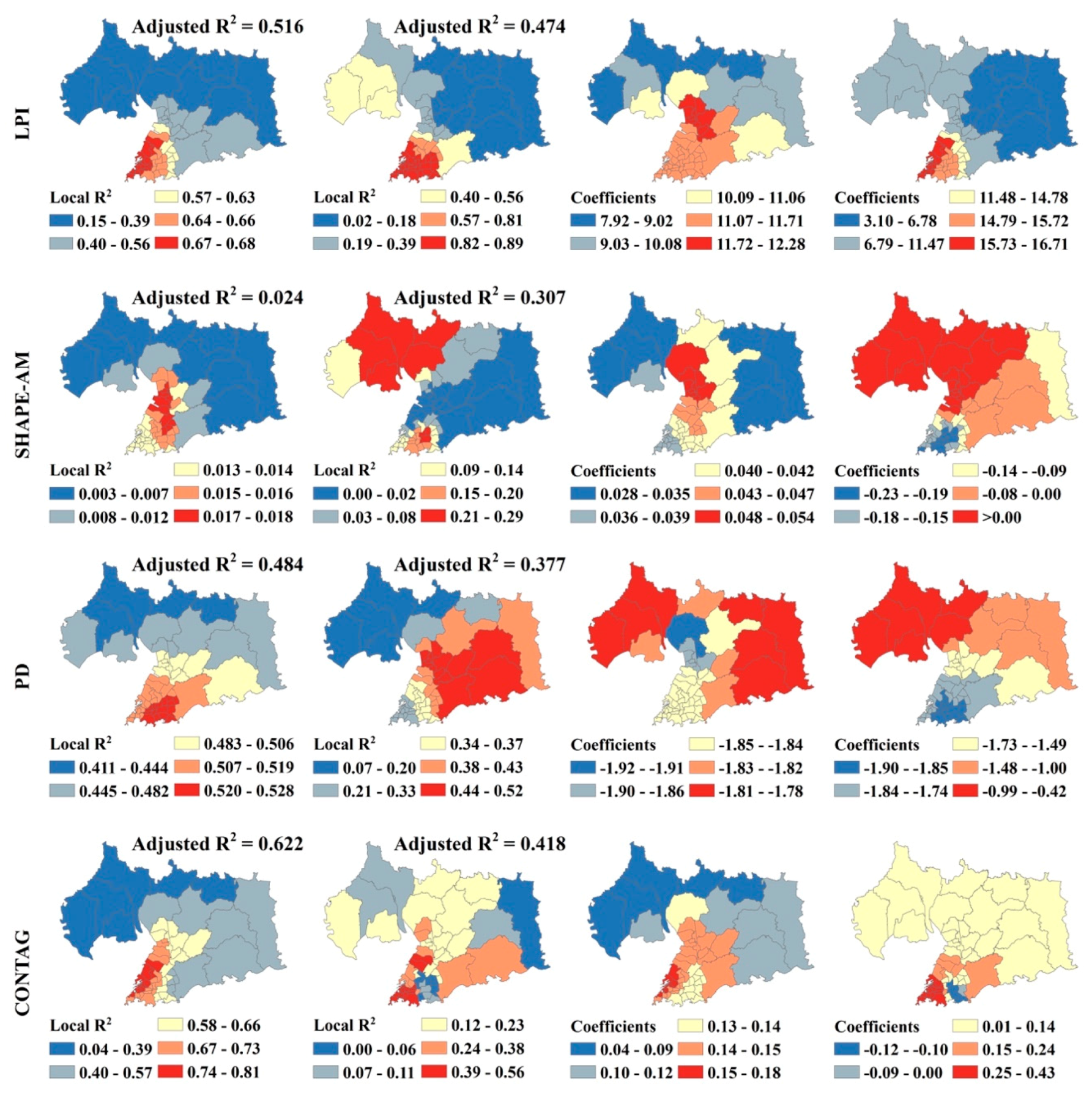
The Pearson’s correlation analysis indicated that the area–edge metrics (LPI) and aggregation metrics (PD and CONTAG) were strongly related to UEI from 1987 to 2016. However, the shape metric (SHAPE-AM) was sensitive to UEI only in the period of 2000–2016.

The spatial relationships between UEI and changes in the landscape metrics at the subdistrict level through GWR are presented in Figure 4. A high explanatory ability of UEI on landscape pattern changes was detected with adjusted R² values ranged from 0.377 to 0.622 for area–edge metrics (LPI) and aggregation metrics (PD and CONTAG). However, this explanatory ability exhibited obvious spatial variations. The highest adjusted R² values shifted from the core urban area in the first stage to the adjacent area where high urbanization was experienced during 2000–2016. It can be concluded that higher urban expansion intensity would explain more landscape pattern changes. The spatial patterns of coefficients revealed that the LPI and CONTAG were positively related, whereas PD was negatively related to UEI in most of the regions from 1987 to 2016.

4. Discussion

4.1. How Much Does Land-Use Change Affect Landscape Patterns?

Changes in land-use could effectively lead to landscape pattern changes [29,50]. The linear regression equations conducted in our study revealed that a strong relationship existed between land-use change and landscape pattern changes (Table 3 and Table 4). This result is similar to the result of Dadashpoor et al. (2019 B) who concluded that landscape pattern changes have a strong relationship with changes in agricultural land, garden land, bare land and built-up land [15]. However, the relationship conducted in our study was varied among different urban development zones and time intervals.

In the downtown area, a 1 km² increase in built-up land caused a 22.801 increase in the LPI and a 0.220 increase in CONTAG from 1987 to 2000, and a 1 km² decrease in forest land was usually accompanied with decreases of 0.504 and 6.439 in SHAPE-AM and PD, respectively (Table 3). In addition, changes in grass land and bare land also contributed to the landscape pattern changes. The reason for this might be that there was no great difference among the changes in these land-use types. However, the dominant influence on landscape patterns was attributed to agricultural land from 2000 to 2016. A 1 km² decrease in agricultural land led to a 25.781 increase in the LPI and caused 18.293 decrease in PD. Meanwhile, the forest land, built-up land and waterbody contributed to the LPI and SHAPE-AM.

In the suburban plain area, the changes in land-use had no significant influence on the four landscape metrics during 1987 and 2000. However, from 2000 to 2016, forest land and agricultural land had a slight influence on landscape pattern change. A 1 km² decrease in forest and agricultural land were usually together with a 0.214 decrease in PD and a 0.047 increase in SHAPE-AM. This may be related to the dispersion of change in forest land. This implied that changes of forest land can fragmentate the landscape [3]. The embezzlement of forest land in the west and the encroachment of built-up land in the center reduced the patch numbers and increased the concentration of patches.

In the mountainous suburban areas, only grassland had a significant effect on changes in SHAPE-AM. A 1 km² decrease in grassland caused a 1.195 increase in SHAPE-AM. This change in the shape properties of the landscape pattern was mainly due to the spatial distribution change in the grassland in this region.

4.2. How Does Urban Expansion Influence Landscape Pattern Changes?

Over the last three decades, the urban expansion in the area has transformed agricultural land, forest land, bare land and so on into built-up land, a transformation which has then led to changes in landscape patterns. The quantitative relationship between them was conducted through the GWR method (Figure 4). Ours findings show that the effect of urban expansion on landscape patterns has spatial and temporal heterogeneity. During the period of 1987–2000, urban expansion was mainly in the form of infilling and edge expansion from the urban core areas. Therefore, UEI has strong explanatory power for landscape patterns among these areas, and the coefficients indicated that the fragmentation level (reflected by PD and the LPI) was significantly, negatively correlated with the intensity of urban expansion. However, in regions far from downtown, the landscape pattern change was relatively less related with urban expansion than the urban core areas. Furthermore, the urban expansion even led to fragmentation in the northwestern area. This agrees with the result of the study of Dadashpoor et al. [15]. They concluded that the growth of built-up lands in a Tabriz metropolitan area has resulted in an increase in aggregation and integration in central and adjacent urban areas, whereas it was opposite in areas far away from built-up lands. Similarly, a few previous studies have also discovered that the expansion of built-up land has reduced the diversity of landscapes and created fragmentation and heterogeneity [1,14,51,52].

From 2000 to 2016, the high explanatory ability has shifted towards suburban areas along with a shift of urban focus, and the correlation coefficients also spatially changed (Figure 4). It can be said that urban expansion has had a significant effect on landscape pattern changes. Chowdhury et al. [4] and Islam [5] also believed that urbanization directly influences the degree of fragmentation in landscapes. Their results also indicated that the built-up landscape has been aggregating in the suburbs where the fragmentation of landscapes was once increased (Table A3 and Figure 4).

Both regression analyses revealed that urbanization has a strong influence on landscape pattern changes, and the effect was different in the three urban development zones. However, the GWR models could give a precise and detailed relationship at each location, which was suitable for questions with spatial heterogeneity [1,53,54].

4.3. Implications

Qingdao has experienced high economic growth since 1990, with an annual growth rate of GDP greater than 6% [38]. This sustained and rapid economic growth has greatly changed the spatial pattern of land-use types in the study area. As a result, a simplified land-use structure has emerged in the downtown area. Meanwhile, the profound influence from urbanization on landscape patterns has been shifting from the city center to the suburbs (Figure 4). According to weak sustainability theory, this region may still be considered sustainable since the total capital of natural and manufactured has increased [7]. However, this sustainability is not sustainable over the long haul. Thus, weak sustainable regions such as well-planned natural areas, agricultural systems and urban centers should be spatially configurated at a large scale in order to reach long-term sustainability, i.e., strong sustainability [6,7,10]. For this purpose, three recommendations are drawn for long-term sustainable development in Qingdao.

Firstly, priority should be given to protect large forest patches and to plant more trees in the downtown. Urban forests play an important role in improving environmental quality and public health in urban areas [55]. Just 20% more trees could double the benefits of urban forests and make cities more environmentally sustainable [50]. In 1987, there are various land-use types in this area, but almost only the forest and construction land have been retained over three decades of urbanization. As a result, the landscape diversity has decreased, and the AI of built-up land has intensified, both of which are not conducive to the sustainable development of urban landscapes. Thus, decision-makers should concentrate on protecting existing forest plots and exploiting new green spaces.

Secondly, the concept of a compact city should be adapted to guide urban planning in the suburban plain area. A compact city is an idea for sustainable urban development to avoid unorderly urban sprawl and achieve harmony between human beings and the natural environment [8,56]. During the process of urban expansion from 1987 to 2016, a large amount of contiguous agricultural land, forest land and water body patches was encroached on by built-up land, leading to a stronger concentration landscape of construction land. Therefore, rational land development strategies, such as establishing limited development zones and retaining large patches of forest and agricultural land with equal distribution, should be made in this region.

Thirdly, anthropogenic disturbances should be continued to be controlled in the suburban mountainous area to protect the forest landscapes and maintain the ecosystem resilience. Due to forest protection policies on Mountain Lao, the forest land area in this region grew from 1987 to 2016 (Table A4). However, it should be noticed that built-up land also had great increases of 179.05% and 149.67% from 1987 to 2000 and from 2000 to 2016, respectively, indicating an increase in anthropic influence. Therefore, decision-makers should focus on setting up prohibited development zones to protect the integrity of the forest ecosystem in this region.

5. Conclusions

This paper aimed to recognize changes in land-use and landscape patterns and to investigate the quantitative influence of land-use change and UEI on landscape patterns in three urban development zones in Qingdao during 1987–2016. For this purpose, firstly, a land-use transform matrix and the landscape metrics of the LPI, SHAPE-AM, PD and CONTAG were used to identify land-use and landscape pattern changes. The results suggested that the growth of the economy in Qingdao has transformed other land-use types such as agricultural and forest land to built-up land in the study area. Therefore, land-use change has caused aggregation and homogeneity in the landscape. Then, a correlation analysis and a stepwise regression were adapted to investigate the quantitative relationship between land-use change and landscape patterns. It has been observed that the influence magnitude of different land-use types on landscape patterns varied for different urban development zones and periods of time. In the downtown area, all the land-use types significantly influenced landscape patterns, and the change in agricultural and forest land had the greatest contribution, especially during the period 2000–2016. However, the agricultural and forest land, respectively, became the dominant factors of landscape pattern changes during 1987–2000 and 2000–2016 in the suburban plain area. The change in grass land had the biggest impact on landscape change in the mountainous suburban areas. Finally, to evaluate urbanization’s impact on landscape pattern changes, GWR regression was used to identify the spatial relationship between UEI and the change in the landscape patterns. The result showed that the effect of UEI on landscape patterns has spatial and temporal heterogeneity. From 1987 to 2000, the UEI strongly explained the change in the landscape patterns and made the landscape assemble faster in the downtown and adjacent areas. However, the a high explanatory ability shifted towards suburban areas during 2000–2016, and the correlation coefficients also spatially changed. The reason for this is the shifting of the focus of urban construction from downtown to the suburbs. Thus, it can be said that UEI has a significant effect on the landscape pattern changes. From this point of view, a compact city and protection policy should be adapted to different regions in the study area to achieve a strong sustainability of urban development.

References

1. Li, H.; Peng, J.; Liu, Y.; Hu, Y. Urbanization impact on landscape patterns in Beijing City, China: A spatial heterogeneity perspective. Ecol. Indic. 2017, 82, 50–60. [Google Scholar] [CrossRef]
2. Zhang, Q.; Su, S. Determinants of urban expansion and their relative importance: A comparative analysis of 30 major metropolitans in China. Habitat Int. 2016, 58, 89–107. [Google Scholar] [CrossRef]
3. Luederitz, C.; Lang, D.J.; von Wehrden, H. A systematic review of guiding principles for sustainable urban neighborhood development. Landsc. Urban Plan. 2013, 118, 40–52. [Google Scholar] [CrossRef]
4. Sahana, M.; Hong, H.; Sajjad, H. Analyzing urban spatial patterns and trend of urban growth using urban sprawl matrix: A study on Kolkata urban agglomeration, India. Sci. Total Environ. 2018, 628–629, 1557–1566. [Google Scholar] [CrossRef] [PubMed]
5. Dadashpoor, H.; Azizi, P.; Moghadasi, M. Analyzing spatial patterns, driving forces and predicting future growth scenarios for supporting sustainable urban growth: Evidence from Tabriz metropolitan area, Iran. Sustain. Cities Soc. 2019, 47, 101502. [Google Scholar] [CrossRef]
6. Bihamta, N.; Soffianian, A.; Fakheran, S.; Gholamalifard, M. Using the SLEUTH Urban Growth Model to Simulate Future Urban Expansion of the Isfahan Metropolitan Area, Iran. J. Indian Soc. Remote Sens. 2014, 43, 407–414. [Google Scholar] [CrossRef]
7. Min, M.; Lin, C.; Duan, X.; Jin, Z.; Zhang, L. Spatial distribution and driving force analysis of urban heat island effect based on raster data: A case study of the Nanjing metropolitan area, China. Sustain. Cities Soc. 2019, 50, 101637. [Google Scholar] [CrossRef]
8. Dadashpoor, H.; Salarian, F. Urban sprawl on natural lands: Analyzing and predicting the trend of land use changes and sprawl in Mazandaran city region, Iran. Environ. Dev. Sustain. 2018. [Google Scholar] [CrossRef]
9. Simwanda, M.; Murayama, Y. Spatiotemporal patterns of urban land use change in the rapidly growing city of Lusaka, Zambia: Implications for sustainable urban development. Sustain. Cities Soc. 2018, 39, 262–274. [Google Scholar] [CrossRef]
10. He, Y.; Song, J.; Hu, Y.; Tu, X.; Zhao, Y. Impacts of different weather conditions and landuse change on runoff variations in the Beiluo River Watershed, China. Sustain. Cities Soc. 2019, 50, 101674. [Google Scholar] [CrossRef]
11. Ali, R.; Bakhsh, K.; Yasin, M.A. Impact of urbanization on CO2 emissions in emerging economy: Evidence from Pakistan. Sustain. Cities Soc. 2019, 48, 101553. [Google Scholar] [CrossRef]
12. Alalouch, C.; Al-Hajri, S.; Naser, A.; Hinai, A. The impact of space syntax spatial attributes on urban land use in Muscat: Implications for urban sustainability. Sustain. Cities Soc. 2019, 46, 101417. [Google Scholar] [CrossRef]
13. Khalil, H.A. Energy Efficiency Strategies in Urban Planning of Cites. In Proceedings of the 7th International Energy Conversion Engineering Conference, Denver, CO, USA, 2–5 August 2009. [Google Scholar]
14. Weng, Y.C. Spatiotemporal changes of landscape pattern in response to urbanization. Landsc. Urban Plan. 2007, 81, 341–353. [Google Scholar] [CrossRef]
15. Dadashpoor, H.; Azizi, P.; Moghadasi, M. Land use change, urbanization, and change in landscape pattern in a metropolitan area. Sci. Total Environ. 2019, 655, 707–719. [Google Scholar] [CrossRef] [PubMed]
16. Shen, S.; Yue, P.; Fan, C. Quantitative assessment of land use dynamic variation using remote sensing data and landscape pattern in the Yangtze River Delta, China. Sustain. Comput. Inform. Syst. 2019, 23, 111–119. [Google Scholar] [CrossRef]
17. Jiao, M.; Hu, M.; Xia, B. Spatiotemporal dynamic simulation of land-use and landscape-pattern in the Pearl River Delta, China. Sustain. Cities Soc. 2019, 49, 101581. [Google Scholar] [CrossRef]
18. Hassan, M.M. Monitoring land use/land cover change, urban growth dynamics and landscape pattern analysis in five fastest urbanized cities in Bangladesh. Remote Sens. Appl. Soc. Environ. 2017, 7, 69–83. [Google Scholar] [CrossRef]
19. Schulp, C.J.E.; Levers, C.; Kuemmerle, T.; Tieskens, K.F.; Verburg, P.H. Mapping and modelling past and future land use change in Europe’s cultural landscapes. Land Use Policy 2019, 80, 332–344. [Google Scholar] [CrossRef]
20. Wan, L.; Zhang, Y.; Zhang, X.; Qi, S.; Na, X. Comparison of land use/land cover change and landscape patterns in Honghe National Nature Reserve and the surrounding Jiansanjiang Region, China. Ecol. Indic. 2015, 51, 205–214. [Google Scholar] [CrossRef]
21. Cabral, A.I.R.; Costa, F.L. Land cover changes and landscape pattern dynamics in Senegal and Guinea Bissau borderland. Appl. Geogr. 2017, 82, 115–128. [Google Scholar] [CrossRef]
22. Qian, J.; Peng, Y.; Luo, C.; Wu, C.; Du, Q. Urban Land Expansion and Sustainable Land Use Policy in Shenzhen: A Case Study of China’s Rapid Urbanization. Sustainability 2016, 8, 16. [Google Scholar] [CrossRef]
23. Liu, X.; Li, X.; Chen, Y.; Tan, Z.; Li, S.; Ai, B. A new landscape index for quantifying urban expansion using multi-temporal remotely sensed data. Landsc. Ecol. 2010, 25, 671–682. [Google Scholar] [CrossRef]
24. Xu, X.; Min, X. Quantifying spatiotemporal patterns of urban expansion in China using remote sensing data. Cities 2013, 35, 104–113. [Google Scholar] [CrossRef]
25. Li, S.; Liu, X.; li, Z.; Wu, Z.; Yan, Z.; Chen, Y.; Gao, F. Spatial and Temporal Dynamics of Urban Expansion along the Guangzhou–Foshan Inter-City Rail Transit Corridor, China. Sustainability 2018, 10, 593. [Google Scholar] [CrossRef]
26. Ren, Z.; He, X.; Zheng, H.; Wei, H. Spatio-Temporal Patterns of Urban Forest Basal Area under China’s Rapid Urban Expansion and Greening: Implications for Urban Green Infrastructure Management. Forests 2018, 9, 272. [Google Scholar] [CrossRef]
27. Sun, X.; Crittenden, J.C.; Li, F.; Lu, Z.; Dou, X. Urban expansion simulation and the spatio-temporal changes of ecosystem services, a case study in Atlanta Metropolitan area, USA. Sci. Total Environ. 2018, 622–623, 974–987. [Google Scholar] [CrossRef]
28. Su, S.; Jiang, Z.; Zhang, Q.; Zhang, Y. Transformation of agricultural landscapes under rapid urbanization: A threat to sustainability in Hang-Jia-Hu region, China. Appl. Geogr. 2011, 31, 439–449. [Google Scholar] [CrossRef]
29. Zhang, W.; Wang, M.Y. Spatial-temporal characteristics and determinants of land urbanization quality in China: Evidence from 285 prefecture-level cities. Sustain. Cities Soc. 2018, 38, 70–79. [Google Scholar] [CrossRef]
30. O’Neill, R.V.; KrummelR, J.R.; Gardner, H.; Sugihara, G.; Jackson, B.; DeAngelis, D.L.; Milne, B.T.; Turner, M.G.; Zygmunt, B.; Christensen, S.W.; et al. Indices of landscape pattern. Landsc. Ecol. 1988, 1, 153–162. [Google Scholar]
31. Matsushita, B.; Xu, M.; Fukushima, T. Characterizing the changes in landscape structure in the Lake Kasumigaura Basin, Japan using a high-quality GIS dataset. Landsc. Urban Plan. 2006, 78, 241–250. [Google Scholar] [CrossRef]
32. Feng, Y.; Liu, Y.; Tong, X. Spatiotemporal variation of landscape patterns and their spatial determinants in Shanghai, China. Ecol. Indic. 2018, 87, 22–32. [Google Scholar] [CrossRef]
33. McGarigal, K.; Cushman, S.; Ene, E. Fragstats V4: Spatial Pattern Analysis Program for Categorical and Continuous Maps. 2012. Available online: http://www.umass.edu/landeco/research/fragstats/fragstats.html (accessed on 2 November 2019).
34. Verburg, P.H.; Veldkamp, A.; Fresco, L.O. Simulation of changes in the spatial pattern of land use in China. Appl. Geogr. 1999, 19, 211–233. [Google Scholar] [CrossRef]
35. Ma, Q.; He, C.; Wu, J.; Liu, Z.; Zhang, Q.; Sun, Z. Quantifying spatiotemporal patterns of urban impervious surfaces in China: An improved assessment using nighttime light data. Landsc. Urban Plan. 2014, 130, 36–49. [Google Scholar] [CrossRef]
36. Tan, M.; Li, X.; Xie, H.; Lu, C. Urban land expansion and arable land loss in China—A case study of Beijing–Tianjin–Hebei region. Land Use Policy 2005, 22, 187–196. [Google Scholar] [CrossRef]
37. Botequilha Leitão, A.; Ahern, J. Applying landscape ecological concepts and metrics in sustainable landscape planning. Landsc. Urban Plan. 2002, 59, 65–93. [Google Scholar] [CrossRef]
38. Zhang, M.; Rasiah, R. Qingdao. Cities 2013, 31, 591–600. [Google Scholar] [CrossRef]
39. Su, S.; Ma, X.; Xiao, R. Agricultural landscape pattern changes in response to urbanization at ecoregional scale. Ecol. Indic. 2014, 40, 10–18. [Google Scholar] [CrossRef]
40. Zha, Y.; Gao, J.; Ni, S. Use of normalized difference built-up index in automatically mapping urban areas from TM imagery. Int. J. Remote Sens. 2003, 24, 583–594. [Google Scholar] [CrossRef]
41. McGarigal, K.; Marks, B.J. FRAGSTATS: Spatial Pattern Analysis Program for Quantifying Landscape Structure; USDA: Washington, DC, USA, 1995.
42. Schindler, S.; Wehrden, H.; Poirazidis, K.; Hochachka, W.M.; Wrbka, T.; Kati, V. Performance of methods to select landscape metrics for modelling species richness. Ecol. Model. 2015, 295, 107–112. [Google Scholar] [CrossRef]
43. Schindler, S.; Poirazidis, K.; Wrbka, T. Towards a core set of landscape metrics for biodiversity assessments: A case study from Dadia National Park, Greece. Ecol. Indic. 2008, 8, 502–514. [Google Scholar] [CrossRef]
44. Plexida, S.G.; Sfougaris, A.I.; Ispikoudis, I.P.; Papanastasis, V.P. Selecting landscape metrics as indicators of spatial heterogeneity—A comparison among Greek landscapes. Int. J. Appl. Earth Obs. Geoinf. 2014, 26, 26–35. [Google Scholar] [CrossRef]
45. Feng, Y.; Liu, Y. Fractal dimension as an indicator for quantifying the effects of changing spatial scales on landscape metrics. Ecol. Indic. 2015, 53, 18–27. [Google Scholar] [CrossRef]
46. Niesterowicz, J.; Stepinski, T.F. On using landscape metrics for landscape similarity search. Ecol. Indic. 2016, 64, 20–30. [Google Scholar] [CrossRef]
47. McGarigal, K. Fragstats v4: Spatial Pattern Analysis Program for Categorical and Continuous Maps-Help Manual. University of Massachusetts, Amherst. 2014. Available online: http://www.umass.edu/landeco/research/fragstats/fragstats.html (accessed on 2 November 2019).
48. Brunsdon, C.; Fotheringham, A.S.; Charlton, M.E. Geographically Weighted Regression: A Method for Exploring Spatial Nonstationarity. Geogr. Anal. 1996, 28, 281–298. [Google Scholar] [CrossRef]
49. Li, S.; Zhao, Z.; Miaomiao, X.; Wang, Y. Investigating spatial non-stationary and scale-dependent relationships between urban surface temperature and environmental factors using geographically weighted regression. Environ. Model. Softw. 2010, 25, 1789–1800. [Google Scholar] [CrossRef]
50. Endreny, T.; Santagata, R.; Perna, A.; de Stefano, C.; Rallo, R.F.; Ulgiati, S. Implementing and managing urban forests: A much needed conservation strategy to increase ecosystem services and urban wellbeing. Ecol. Model. 2017, 360, 328–335. [Google Scholar] [CrossRef]
51. Herold, M.; Goldstein, N.C.; Clarke, K.C. The spatiotemporal form of urban growth: Measurement, analysis and modeling. Remote Sens. Environ. 2003, 86, 286–302. [Google Scholar] [CrossRef]
52. Abdullah, S.A.; Nakagoshi, N. Changes in landscape spatial pattern in the highly developing state of Selangor, peninsular Malaysia. Landsc. Urban Plan. 2006, 77, 263–275. [Google Scholar] [CrossRef]
53. Fotheringham, A.S.; Brunsdon, C.; Charlton, M.E. Geographically Weighted Regression: The Analysis of Spatially Varying Relationships; Wiley: New York, NY, USA, 2002. [Google Scholar]
54. Su, S.; Xiao, R.; Zhang, Y. Multi-scale analysis of spatially varying relationships between agricultural landscape patterns and urbanization using geographically weighted regression. Appl. Geogr. 2012, 32, 360–375. [Google Scholar] [CrossRef]
55. Gerrish, E.; Watkins, S.L. The relationship between urban forests and income: A meta-analysis. Landsc. Urban Plan. 2018, 170, 293–308. [Google Scholar] [CrossRef]
56. Jim, C.Y. Sustainable urban greening strategies for compact cities in developing and developed economies. Urban Ecosyst. 2013, 16, 741–761. [Google Scholar] [CrossRef]
Figure 1. The location (A), three types of urban development zones in 2016 (B), and the terrain as well as main road (C) of the study area.
Sustainability 11 06174 g001
Figure 2. Land-use/cover maps in 1987, 2000, and 2016 in study areas.
Sustainability 11 06174 g002
Figure 3. Changes of four landscape metrics in different urban development zones during 1987–2016. LPI: largest patch index; SHAPE-AM: area-weighted mean shape index; PD: patch density; CONTAG: contagion.
Sustainability 11 06174 g003
Figure 4. Spatial distribution of local R2 value and correlation coefficients between urban expansion intensity and landscape metrics during 1987–2000 (the first and third columns) and 2000–2016 (the second and fourth column) acquired from geographically weighted regression (GWR) models. The Jenks Natural Breaks classification method was used, and 0 was set as the bread value when the value of coefficients crossed it.
Sustainability 11 06174 g004