A Novel Intelligence Approach of a Sequential Minimal Optimization-Based Support Vector Machine for Landslide Susceptibility Mapping

Abstract

The main objective of this study is to propose a novel hybrid model of a sequential minimal optimization and support vector machine (SMOSVM) for accurate landslide susceptibility mapping. For this task, one of the landslide prone areas of Vietnam, the Mu Cang Chai District located in Yen Bai Province was selected. In total, 248 landslide locations and 15 landslide-affecting factors were selected for landslide modeling and analysis. Predictive capability of SMOSVM was evaluated and compared with other landslide models, namely a hybrid model of the cascade generalization optimization-based support vector machine (CGSVM), individual models, such as support vector machines (SVM) and naïve Bayes trees (NBT). For validation, different quantitative criteria such as statistical based methods and area under the receiver operating characteristic curve (AUC) technique were used. Results of the study show that the SMOSVM model (AUC = 0.824) has the highest performance for landslide susceptibility mapping, followed by CGSVM (AUC = 0.815), SVM (AUC = 0.804), and NBT (AUC = 0.800) models, respectively. Thus, the proposed novel SMOSVM model is a promising method for better landslide susceptibility mapping and prediction, which can be applied also in other landslide prone areas.

1. Introduction

Landslide susceptibility mapping is an appropriate tool for management of landslide hazards [1]. Landslide susceptibility of an area is usually assessed based on the analysis of spatial relationship of historical landslide occurrences with the number of affecting factors [2]. Occurrence of landslides depends on the characteristics of the study area such as geology, topography, soil, and other geo-environmental factors. In addition, analysis of the natural mechanism of landslides helps in the assessment and management of landslides [3].

Challenge to modeling landslides is the uncertainty issue including inputs, landslide conditioning factors, and model selection [4]. As there is no standard guideline and framework to select the number of landslide conditioning factors, the users based on the literature and data availability of a given study area select the factors for the modeling process. Although there are some factor selection techniques to determine the best factors in the modeling, another uncertainty is model selection that affects the goodness-of-fit and prediction accuracy of the models [4]. It is apparent that some methods and techniques have been developed; however, all of them are not applicable in all regions. Therefore, each model firstly should be tested and evaluated for specific area and then to be used for modeling process. Basically, the main aim of landslide researchers is to select the best factors and models in order to decreases the uncertainties during modeling process for enhancing the power prediction of the models.

In recent decades, a number of conventional and statistical methods/models are used for the landslide susceptibility mapping such as: (i) conventional models: analytic hierarchy process (AHP) [5,6]; (ii) bivariate models: weights-of-evidence (WOE), information value (IV), fuzzy logic (FL), statistical index (SI), frequency ratio (FR), and certainly factor (CF) [7,8,9,10,11,12,13]. Nowadays, machine learning (ML) models are considered better than conventional and statistical models in landslides studies [14,15]. Some of these models are adaptive neuro-fuzzy inference system (ANFIS), artificial neural network (ANN), support vector machines (SVM), logistic regression (LR) [16,17,18,19,20,21], and decision tree-based algorithms: alternating decision tree (ADT), logistic model tree (LMT) [4,18,22,23,24,25], Bayes-based algorithms: Bayesian logistic regression (BLR), and naïve Bayes (NB) [23,26,27,28]. In general, these ML methods are promising approaches for landslide susceptibility assessment and mapping as they are based on computational algorithms which can mine and analyze the data effectively in solving the complex relationship between landslide incidents and many input landslide affecting factors.

In recent years, instead of single ML models, hybrid models are developed and applied for landslide susceptibility mapping for better accuracy of landslide prediction. These hybrid models include ANFIS coupled with a genetic algorithm (ANFIS-GA) [29,30], ANFIS coupled with differential evolution (ANFIS- DE) [29], ANFIS combined with biogeography-based optimization and BAT algorithms (ANFIS-BBO and ANFIS-BAT) [31], ANFIS combined with an imperialistic competitive algorithm (ANFIS-ICA) and firefly algorithm (ANFIS-FA) [32], naïve Bayes trees (NBT) classifier coupled with random subspace ensemble (RS-NBT) [26], alternative decision trees combined with various ensemble methods [24], and the radial basis function neural network coupled with rotation forest (RBFRF) [33]. Generally, these hybrid ML techniques show promising alternative approaches compared with single ML approaches as their combination or integration usually gives better performance than using each individual machine learning or decision-making model alone. Hybrid models take advantages of individual ML methods; thus, they can learn the data more deeply and discover more accurately the relationship hidden in complex problems such as landslides.

In this study, the main objective is to apply a novel hybrid ML model named sequential minimal optimization-based support vector machines (SMOSVM), which is a combination of sequential minimal optimization (SMO) and SVM for accurate mapping of landslide susceptibility at the Mu Cang Chai District, Yen Bai province, which is one of the high landslide prone areas of Vietnam. Out of these methods, SVM is known as a benchmark single model and as one of the powerful classifiers which is widely used for classification problems in general and in landslide prediction in particular [34,35,36]. However, SVM has a disadvantage that it is not applicable for large and complex datasets as it uses inequality constraints to solve large scale quadratic programming problems arising during learning process which leads to great computational complexity [37]. Therefore, Platt [38] proposed SMO which can be used to overcome the limitations of SVM, and it can decrease the over-fitting and noise problems in training dataset [39]. Therefore, it is considered that hybrid model in combination of SMO with SVM can be faster and more effective in solving the prediction problems. This approach is based on the assumption that the problem of large quadratic programming in SVM could be divided into a series of the smallest possible problems that could be tackled analytically using two Lagrange multipliers per step [38]. Even though this approach is promising, so far its predictive capability has not been verified for landslide susceptibility mapping. Performance of the new hybrid model was validated and compared with single SVM, NBT models and a new hybrid model, namely Cascade Generalization Optimization-based SVM (CGSVM), using statistical based methods and receiver operating characteristic curve technique. Weka 3.9 (www.cs.waikato.ac.nz) and ArcGIS 10.3 software (ESRI, Redlands, CA, USA) were used for data processing and development of landslide susceptibility maps.

2. Data Acquisition

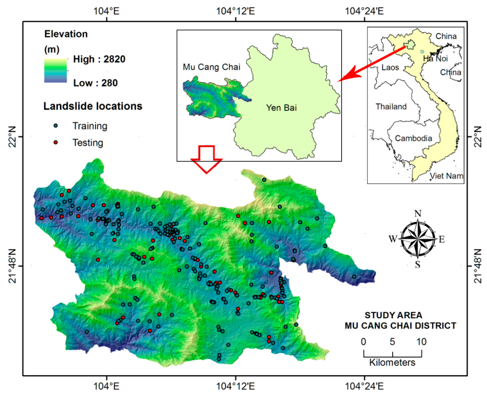
2.1. Description of the Study Area

The Mu Cang Chai District, which is one of the landslide prone area of Vietnam, located in the northwest part of Yen Bai Province was selected as a study area (Figure 1). This district is located between latitudes 21°39′00″ N to 21°50′00″ N and longitudes 103°56′00″ E to 104°23′00″ E, covering an area of approximately 1196 km². The population of the Mu Cang Chai District in 2010 was 50,107 people, with a population density of about 42 people per km². Climate of this area is temperate, tropical monsoon type. Rainfall in the area is relatively high, which varies from 3700 mm to 5490 mm and humidity about 81%. Annual temperature varies from 9.7 °C (December/January) to 28 °C (June/July). Majority of the area is covered by forest (61.76%), followed by barren lands, cultivated lands, residential area, and scrub lands.

Topography of the area is dominated by elongated ridges (hills) and intervening valleys. Elevation ranges from 280 m to 2820 m with mean elevation 1515 m. Mountain slopes are relatively steep, up to 88 degrees. A major part of the area is occupied by extrusive and intrusive magmatic (volcanic) rocks. Metamorphic and sedimentary rocks are also present in this area. Tectonically, the area is still active, as evident by earthquake activities.

2.2. Data Acquisition and Analysis

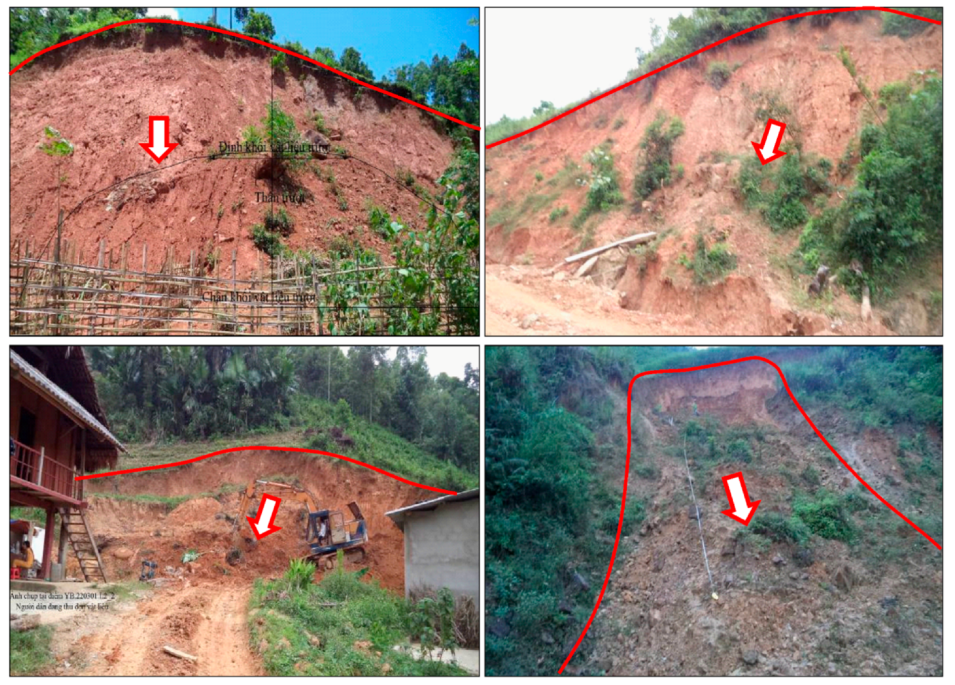
2.2.1. Landslide locations

Landslide locations were recorded from aerial photographs (scale 1:33,000), Google Earth images, and field surveys. Validation of the landslide events was done in the field under the Vietnam Institute of Geosciences and Mineral Resources (VIGMR) national project named “Survey, assessment and zoning of landslide warning in the mountainous region of Vietnam” (Figure 2). In total 248 landslide locations were identified to construct landslide inventory map (Figure 1). The landslide inventory was used to assess the spatial relationship between landslide events and landslide conditioning factors. Five types of landslides observed in this area namely rotational (124 events), mixed (36 events), translational (35 events), toppling (45 events), and debris slides (eight events). Most of landslides in this area are triggered by heavy rains during monsoon.

2.2.2. Landslide Influencing Factors

Landslide affecting factors which depend on the local topography, geology, meteorology, and other geo-environmental factors, such as slope, elevation, aspect, curvature, plan curvature, profile curvature, land use, lithology, distance to faults, distance to roads, distance to rivers, fault density, road density, river density, and rainfall, were selected for landslide susceptibility analysis in this study. For evaluating relationship of these factors with landslide events, Frequency ratio (FR) analysis was performed based on number of landslide pixels per number of pixels of each class of the affecting factor [6].

Aspect is defined as the direction of slopes faces [3] which affects the precipitation and solar radiation [40,41]; thus, it affects landslide occurrences [3]. Thus, an aspect map was prepared from a Digital Elevation Model (DEM) with 20 m spatial resolution which was generated from topographical map at the scale of 1: 500,000 ollected from the VIGMR, and classified into nine classes (Figure 3a). The highest FR values of landslide occurrence were obtained for southwest (FR = 1.2) slopes. Other slopes (west, south, and east slope with FR > 1 were also observed susceptible to landslide occurrences due to combination of other geo-environmental factors (Figure 4).

Curvature of a terrain surface controls flow of the water thus affects landslide incidences [42,43]. Positive values of curvature reflect concave surface, negative values reflect convex surface, and near-zero values indicate flat area [44]. Landslides have more frequency in concave surface than convex surface due to accumulation of water [45]. Curvature map was generated from DEM with three classes: concave (<−0.05), flat (−0.05–0.05), and convex (>0.05) (Figure 3b). Frequency analysis indicates that curvature having an FR value of 1.2 is more prone to landslides (Figure 4).

Fault density which is defined as the ratio of the length of the total faults to a given area, is also considered as one of the affecting factor to landslide occurrences [46]. This map was generated using kernel density function of ArcGIS. A fault density map was classified into five classes using the “Quantile” method [47] (Figure 3c). The FR values suggest that there is a small relationship between landslide occurrences and fault density in the present case (Figure 4).

Distance to faults is an important conditioning factor to landslide occurrences as faults create instability in groundmass causing landslides [41,48,49]. Faults, in the present study, were extracted from the national geological maps (1: 50,000 scale) obtained from the VIGMR. Buffer maps of faults distances were generated in seven classes: 0–100, 100–200, 200–300, 300–400, 400–500, 500–600, 600–700, and >700m (Figure 3d). In the study area, there is no direct relation between FR values with fault distances which suggest that the orientation and nature of faults are not unfavorable to slope stability (Figure 4).

River density which is defined as the ratio of the length of the total river network to a given area, is also considered as an important affecting factor to landslide occurrences [46]. Similar to the distance to rivers, the river density map was generated by kernel density function using GIS software. River density map was classified using the “Quantile” method in five classes: very low, low, moderate, high, very high (Figure 3e) [47]. Moderate (FR = 1.4) and low (FR = 1.2) river density classes have higher FR values and, thus, more prone to landslides (Figure 4).

Distance to rivers is important factor in landslide occurrences due to direct effect of slope erosion and increase in ground mass moisture [50]. Seepage and surface runoff also flows on valley faces from hilltop to riverbed increasing possibility of landslides. The river network, in the present study, was extracted from topographic maps on 1: 50,000 cale and classified into five classes: 0–50, 50–100, 100–150, 150–200, 200–250, and >250 m (Figure 3f). The lowest and the most susceptible classes of distance to rivers in the study area are 50–100 m (FR = 0.69) and 150–200 m (FR = 1.8), respectively (Figure 4).

Road density is defined as the ratio of the length of the total road network to a given area. This factor is also important in landslide occurrences [46]. It was extracted by kernel density function using GIS application. Road density maps were classified using the “Quantile” method [47]: very low, low, moderate, high and very high (Figure 3g). Unlike the relationship between the distance to roads and FR values, in the road density there is a direct trend between the road density and FR values. Higher values of road density indicates higher values of FR and, thus, higher susceptibility to landslide occurrence. Accordingly, high and very high class of road density commonly have the higher values of FR (2.4), thus, these areas are more prone to landslides incidences (Figure 4).

Distance to roads is one of the important affecting factor to landslide occurrences as excavation for roads disturb the slope forming materials [51]. In this study, a total of 861 road sections aggregating 914.987 km were extracted from topographic map at a 1: 50,000 scale. However, only road sections on slope angles higher than 10 degrees were used to prepare distance to roads map in five classes: 0–50, 50–100, 100–150, 150–200, 200–250, and > 250 m (Figure 3h). The FR values and distance to roads conditioning factor are having reverse relationships, the FR values are increasing with the reduction of distance from roads (Figure 4). Higher value of FR (5.7) was obtained for the class of 0–50 m distance to road in the study area.

Slope is one of the most important factors for landslide incidence [41,52,53,54]. However, it should be considered in relation with the slope materials to analyze landslide occurrences as the shear resistance of the slope of unconsolidated materials decreases as slope angles increase [3]. Normally, landslides have high FR in moderate slopes (30–40 degree) [40]. A slope map of the study area was generated from DEM with several classes: 0–10 (FR = 0), 10–20 (FR = 1.7), 20–30 (FR = 1.1), 30–40 (FR = 0.86), 40–50 (FR = 0.62), and >50° (FR = 0.66) (Figure 3i and Figure 4).

Rainfall is one of the triggering factors for landslide occurrences in the northern part of Viet Nam including the study region [55,56]. Rainfall decreases the shear resistance of ground/rock mass due to saturation [41,57]. Rainfall map of the study region was generated using rainfall data of 31 years (1984 to 2014) obtained from Global Weather data for SWAT [41,58] and classified into different classes based on annual average rainfall: 3771–4000, 4000–4250, 4250–4500, 4500–4750, 4750–5000, 5000–5250, and 5250–5491 mm (Figure 3j). Analysis of the FR data indicates that the threshold value of landslide occurrences (FR = 1) is at lower rainfall values (4000–4250 mm), therefore, higher rainfall values are not increasing the landslide events as the slopes already failed at lower values (Figure 4).

Profile curvature presents the rate of slope change over each terrain unit [44]. Profile curvature map was derived from the DEM into different classes (Figure 3k). The FR analysis indicates that the class: [(−52.003)–(−9.183)] is most susceptible to landslide occurrences (Figure 4).

Plan curvature indicates terrain surface bending on slope in perpendicular direction [44] affecting the stability of slopes in hilly areas. Plan curvature map was generated from DEM in different classes (Figure 3l). Plan curvature class: [(−334.189)–(−69.843)] has the highest value of FR, suggesting that this class is more prone to landside occurrences than other classes.

Lithology plays an important role in landslide occurrences as different types of rocks have different geo-mechanical properties affecting the stability of slopes [41,57,59]. Generally, metamorphic and sedimentary rocks have more frequency of landslide occurrences than igneous rocks due to presence unfavorable discontinuities [41]. A lithology map of the study area was generated from the Geological and Mineral Resources Map of the Mu Cang Chai District on 1:50,000 scale. Different lithological groups present in the area include group 1 (igneous magmatic rocks), group 2 (intrusive magmatic rocks), group 3 (sedimentary rocks), group 4 (mafic-ultramafic magma rocks), group 5 (carbonate rocks), and group 6 (quaternary deposits). These groups are based on estimated strength, degree of weathering, and mineral composition [60,61] (Figure 3m). The FR value reveals that group 1 (FR = 1.1) of lithology has the most potential for landslide occurrence in this area (Figure 4).

Land use pattern affects the stability of slopes depending on its use for cultivation, forest, building, vacant, or barren land. Anthropogenic activities also disturb the natural environment of ground slope [40]. Land use map of the study area was generated using air photos on 1:33,000 scale and classified into five classes: barren land, cultivated land, forestland, residential area, and scrubland (Figure 3n). The FR values indicate that residential areas (FR = 4.4) and cultivated lands (FR = 2.4) are most susceptible to landslide occurrences in comparison to other classes (FR < 1).

Elevation affects weathering and shear strength of slope forming material [41]. Rocks occurring at higher elevations are generally less weathered due to geo-environmental factors. Thus, landslides often have less frequency in very high elevation areas. Elevation map was generated from DEM in different classes: 280–700, 700–900, 900–1100, 1100–1300, 1300–1500, 1500–1700, 1700–1900, 1900–2100, 2100–2300, and >2300 m (Figure 3o). The FR values for these classes are 0.84, 2.2, 1.9, 2.3, 0.98, 0.73, 0.38, 0, 0.14, and 0.18, respectively. Frequency analysis indicates that the elevation class of 1100–1300 is the most susceptible for landslide incidence (Figure 4).

2.3. Dataset Generation

Training and testing datasets were generated training and validating models [63]. In the present study, landslide locations were randomly classified into two sets: (1) 70% landslide location for training dataset; and (2) 30% landslide locations for testing dataset using random data classification tool of ArcGIS. The ratio of random classification was decided based on the standard practice mentioned in the literature [63]. Data conversion in 20 × 20 m pixel size was done to maintain the uniformity with other layers. A separate dataset of non-landslide points was also extracted from non-landslide areas for the analysis. More specifically, 174 landslide points and 174 non-landslide points were used to generate training dataset, 74 landslide points and 74 non-landslide points were utilized to generate testing dataset. Finally, landslide-affecting factor maps were used to sample with these landslide and non-landslide points for generating the final datasets for further processing in models.

3. Methods Used

3.1. Support Vector Machines (SVM)

SVM was introduced by Vapnik [64], which is known as one of the best classifiers for solving many real classification problems including landslides [14]. The main principle of SVM is to find the optimal hyper-plane to classify two variables of binary classification problems [63]. This hyper-plane in a three-dimensional space can classify the landslide and non-landslide points. The SVM function fits some hyper-planes and then the best one with the lowest classification error is selected and performed to final classify landslide and non-landslide points. For landslide prediction, suppose (x, y) is a vector of training dataset whereas x = x_i, i = 1, 2, …, m represents landslide influencing factors (m is the number of factors), and y = (1, 0) represents classified variables (landslide and non-landslide). The optimal hyper-plane can be found during training process of the SVM as following expression [64]:

$$f\left(x\right)=sign\left[{\displaystyle \sum _{i=1}^m{\epsilon }_i{y}_{j}k\left(x,x_i\right)+b}\right]$$

(1)

where $b$ is defined as the offset from the origin of the hyper-plane, $k\left(x_i,x_j\right)$ are kernel functions which are defined as infinite dimensional feature spaces [65].

Using above Equation, the hyper plane is generated to divide two labels (landslide, and non-landslide) for classification, and it also causes the quadratic programing problems as following [64]:

$$\begin{array}{l}Maxi\min e:R({\alpha }_i)={\displaystyle \sum _{i=1}^m{\epsilon }_i-\frac{1}{2}}{\displaystyle \sum _{i=1}^m{\displaystyle \sum _{j=1}^m{\epsilon }_i{\epsilon }_j}}{y}_i{y}_{j}k(x_i,x_j)\\ Subjectto:{\displaystyle \sum _{i=1}^m{\epsilon }_i{y}_i}=0vs0\le {\epsilon }_i\le C,i=1,2,\dots ,m\end{array}$$

(2)

where C is the complexity parameter that controls the trade-off between allowance and maximizing margin for misclassification [66]; ${\epsilon }_i$ are positive real constants [67].

3.2. Sequential Minimal Optimization (SMO)

SMO is known as an efficient algorithm for solving the quadratic programming problems arises during training process of SVM. It was applied widely for training SVM especially for complex problems with large and complicated datasets [38]. During the SVM learning process, SMO is applied simultaneously to optimize the quadratic programming problems that has the penalty for misclassification, as shown in Equation (2) [66]. In other words, SMO is an algorithm that optimizes the result of the SVM classification algorithm. It is possible to misclassify some cases of landslides during the training process by the SVM model. To avoid this error during training, SMO, which uses the optimal quadratic programming problems, leads to accurate selection of the best hyper-plane for classifying landslide and non-landslide points. Therefore, SMO decreases the misclassification of SVM and, hence, improves the goodness-of-fit and thus prediction accuracy. It can be carried out in two main steps:

(1)

To identify and solve analytically the two Lagrange multipliers, at first, the constrained maximum value is obtained by the calculation of the constraints on the two Lagrange multipliers, and the constraint $0\le {\beta }_i\le C$ is utilized to restrict two Lagrange multipliers within a diagonal line [68]. Lagrange multipliers are then shifted to the point with the lowest value of the objective function [68].

(2)

To choose suitable Lagrange multipliers using heuristics for optimizing the quadratic programming problems [38], two heuristics are utilized to choose two suitable Lagrange multipliers [38]. One heuristic is employed to train all samples in the first multiplier and identify those that do not satisfy the Karush–Kuhn–Tucker (KKT) conditions [38]. A second heuristic is utilized to maximize approximately the size of the previous step in the second multiplier during the optimization process. Suitable Lagrange multipliers are selected based on selection of the sample having the largest error difference from the previous sample [68].

3.3. Cascade Generalization (CG)

CG, proposed in 2000, has been extensively employed in domains of ensemble learning [69,70,71,72]. Different from conventional stacking algorithm consisting of multiple levels, in the procedure of CG algorithm, the outputs of base level are utilized to generate new features to samples in original data for the purpose of extending input space [73]. Therefore, CG can be considered as a sequential framework, which is used to integrate various classifiers while stacking is parallel. Additionally, CG possesses other merits as well, including that even classifiers on intermediate levels have access to the original attributes, and the computational efficiency is significantly enhanced without internal cross validation [39]. It should be also noted that there exist two cascade generalization schemes, respectively, loose coupling and tight coupling schemes [69].

Suppose that the original training data D can be expressed as the following form:

$$D=\left\{(y_m,X_m),m=1,\cdots ,M\right\}$$

(3)

where y_m is the corresponding class label of the m-th sample. X_m represents the original attribute vector of the m-th sample. M is the total number of samples.

The metadata produced by inputting original training data D into the base level classifiers can be described as below:

$$D_{\mathrm{L}1}=\left\{(X_m,y_m,C_m),m=1,\cdots ,M\right\}$$

(4)

where C_m denotes the vector of predictive classes which are generated by various base level classifiers.

When addressing binary classification problems, Equation (4) can be rewritten as follows if these base level classifiers output conditional probability distributions:

$$D_{\mathrm{L}1}=\left\{(X_m,p_{\mathrm{n}}{c}_{1m},p_{\mathrm{p}}{c}_{1m},\cdots ,p_{\mathrm{n}}{c}_{km},p_{\mathrm{p}}{c}_{km},y_m),m=1,\cdots ,M\right\}$$

(5)

where p_n and p_p mean the probability distributions of negative and positive classes namely. c_km represents the predictive class derived from the k-th base level classifier.

CG can improve performance of the base classifier by decreasing the bias in training dataset [39]. CG belongs to the family of stacking generalization algorithms [74]. The training is done by this technique at two or more levels including: (i) a learning algorithm is used to combine the outputs of the base classifier (SVM). The original training dataset constitutes the level zero data; however, level one is the outputs of the base classifier and (ii) the level one dataset is used to prepare the final classification. Eventually, the final results can be obtained by processing the metadata on multiple learning levels using the aforementioned procedure. In other words, at this stage the results of classification by base classifiers (such as SVM) are combined to obtain the final decision [39].

3.4. Naïve Bayes Trees (NBT)

NBT, belonging to the family of decision tree algorithms, is known as a combination of naïve Bayes theory and decision tress [75]. In terms of the NBT structure, the most significant feature is that naïve Bayes classifier is adopted on each leaf node and decision trees is adopted on each node [76]. For landslide prediction, suppose (x, y) is a vector of training dataset whereas x = xi, i = 1, 2, …, m represents landslide influencing factors (m is the number of factors), and y = (1, 0) represents classified variables (landslide and non-landslide). In this model, firstly, the tree is grown using a decision tree algorithm. A landslide conditioning factor with the highest entropy is selected as the root and then the tree will be divided and nodes appear. When all landslide examples are labeled to their classes the algorithm is stopped and the leaf nodes are created. Consequently, a naïve Bayes algorithm is constructed for each leaf using the data associated with that leaf. Finally, the probability values for each pixel of training and then for all pixels of study area are assigned and computed to prepare landslide susceptibility map. Specifically, the NBT classifier can be implemented using the following formula [77]:

$$t_{\mathrm{NB}}=\underset{z_i}{\arg \max }\mathrm{PP}(t_i){\displaystyle \prod _{i=1}^m\frac{1}{\sqrt{2\pi \epsilon }}}{e}^{\frac{-{(r_i-\sigma )}^2}{2{\epsilon }^2}}$$

(6)

where PP(t_i) refers to the prior probability of the output variables t_i = (1, 0). r_i is the i-th attribute in training dataset. σ and ε correspondingly denote the mean value and standard deviation of r_i.

In the process of establishing decision trees, the gain ratio (GR) values are calculated by Equation (7) in an effort to control tree growth [78]:

$$GR=\frac{Entropy(U)-{\displaystyle \sum _{i=1}^m\frac{\left|U_i\right|}{\left|U\right|}Entropy(U_i)}}{-{\displaystyle \sum _{i=1}^m\frac{\left|U_i\right|}{\left|U\right|}{\log }_2\frac{\left|U_i\right|}{\left|U\right|}}}$$

(7)

where U represents the training dataset in this case.

3.5. Evaluation and Comparison Methods

For validation, two quantitative methods were applied, namely the statistical index (SI)-based method and the receiver operating characteristic (ROC) curve method. These two methods are applied widely to validate the performance of the models [14,43,79]. The SI-based method is the evaluation based on the values of statistical indexes such as sensitivity (SST), specificity (SPF), accuracy (ACC), kappa, and root mean squared error (RMSE). SST shows the degree of success of the model in correctly classifying the number of landslides pixels whereas SPF shows the degree of success of the model in correctly classifying the number of non-landslide pixels [14]. ACC indicates the degree of success of the model in correctly classifying the number of landslides and non-landslide pixels (the general performance of the landslide model). Kappa shows how reliable the model is for landslide prediction. RMSE shows how accurate the model is for landslide classification [80]. Higher the values of SST, SPF, ACC, and kappa show better performance of landslide models. Lower values of RMSE indicate better predictive capability of landslide models [14]. These statistical indices can be calculated using four types of possible consequences, including true positive (TP), true negative (TN), false positive (FP), and false negative (FN) as shown by the following equations [81]:

$$\mathrm{PPV}=\frac{\mathrm{TP}}{\mathrm{FP}+\mathrm{TN}};\mathrm{NPV}=\frac{\mathrm{TN}}{\mathrm{FN}+\mathrm{TN}};\mathrm{SST}=\frac{\mathrm{TP}}{\mathrm{TP}+\mathrm{FN}};\mathrm{SPF}=\frac{\mathrm{TN}}{\mathrm{TN}+\mathrm{FP}};\mathrm{ACC}=\frac{\mathrm{TP}+\mathrm{TN}}{\mathrm{TP}+\mathrm{TN}+\mathrm{FP}+\mathrm{FN}}$$

(8)

$$Kappa=\frac{P_c-P_{\exp }}{1-P_{\exp }}=\frac{(TP+TN)/(TP+TN+FP+FN)}{1-[((TP+TN)(TP+FP))+((FP+TN)(FN+TN))/\sqrt{TP+TN+FP+FN})]}$$

(9)

$$\mathrm{RMSE}=\sqrt{\frac{1}{\mathrm{n}}}{\displaystyle \sum _{\mathrm{i}=1}^{\mathrm{n}}{(\mathrm{X}}_{\mathrm{Pred}.}{-\mathrm{X}}_{\mathrm{act}.}}{)}^2$$

(10)

where $P_{\exp }$ is expected agreements, ${\mathrm{X}}_{\mathrm{Pred}.}$ is the predicted values in the training dataset or the validation dataset; ${\mathrm{X}}_{\mathrm{act}.}$ is the actual values from the landslide susceptibility model and $n$ is the total samples in the training dataset or the validation dataset.

ROC curve is a graphical measure to assess the overall performance of prediction models [82,83]. It is plotted in a two-dimensional space using the SST and 100-SPF on the x-axis and y-axis, respectively [84,85]. To assess the general performance of a given model, the area under the ROC curve (AUC) is used [86]. Mathematically, higher AUC metric indicate better performance of a given model. A model with AUC equals to 0.5 is an inaccurate model (random accuracy model); however, a value of 1 indicates a perfect model [87].

3.6. Linear Support Vector Machine (LSVM) Feature Selection

In spatial prediction modeling, selection of appropriate input factors is one of the most important steps and on the other hand there is no global guideline for the selection of landslide conditioning factors [88]. In the present study, LSVM was applied for the selection of the proper conditioning factors using the following equation [89,90]:

$$g(x)=\mathrm{sgn}(w^{T}m+n)$$

(11)

where $m=(m_1,m_2,m_3,\cdot \cdot \cdot ,m_{12})$ is the input vector containing the factors, $w^T$ is the inverse matrix, and n is the offset from the origin of the hyper-plane [89].

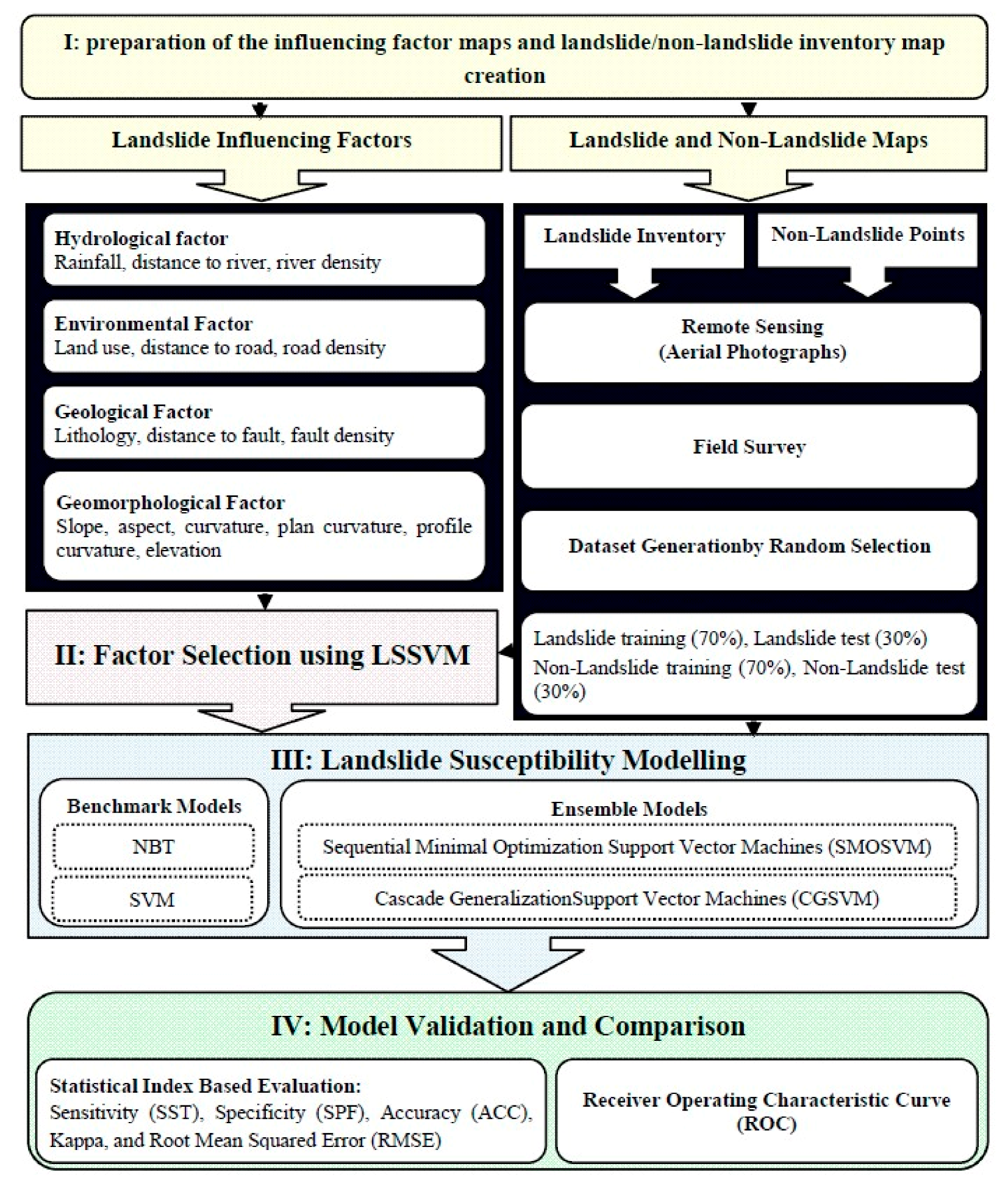
3.7. Methodological Flow Chart and Steps

In the current research two novel classifier ensemble methods, namely SMOSVM and CGSVM models, were applied for the development of landslide susceptibility maps. SMOSVM is a hybrid approach of SMO and SVM models and the CGSVM model is constructed based on CG and SVM. Performance of the SMOSVM and CGSVM models were compared with other single benchmark models (SVM and NBT). The current study was conducted in four main steps: (I) preparation of the influencing factor maps and landslide/non-landslide inventory map, (II) factor selection using LSVM, (III) landslide susceptibility modelling, and (IV) model validation and comparison (Figure 5).

4. Results and Analysis

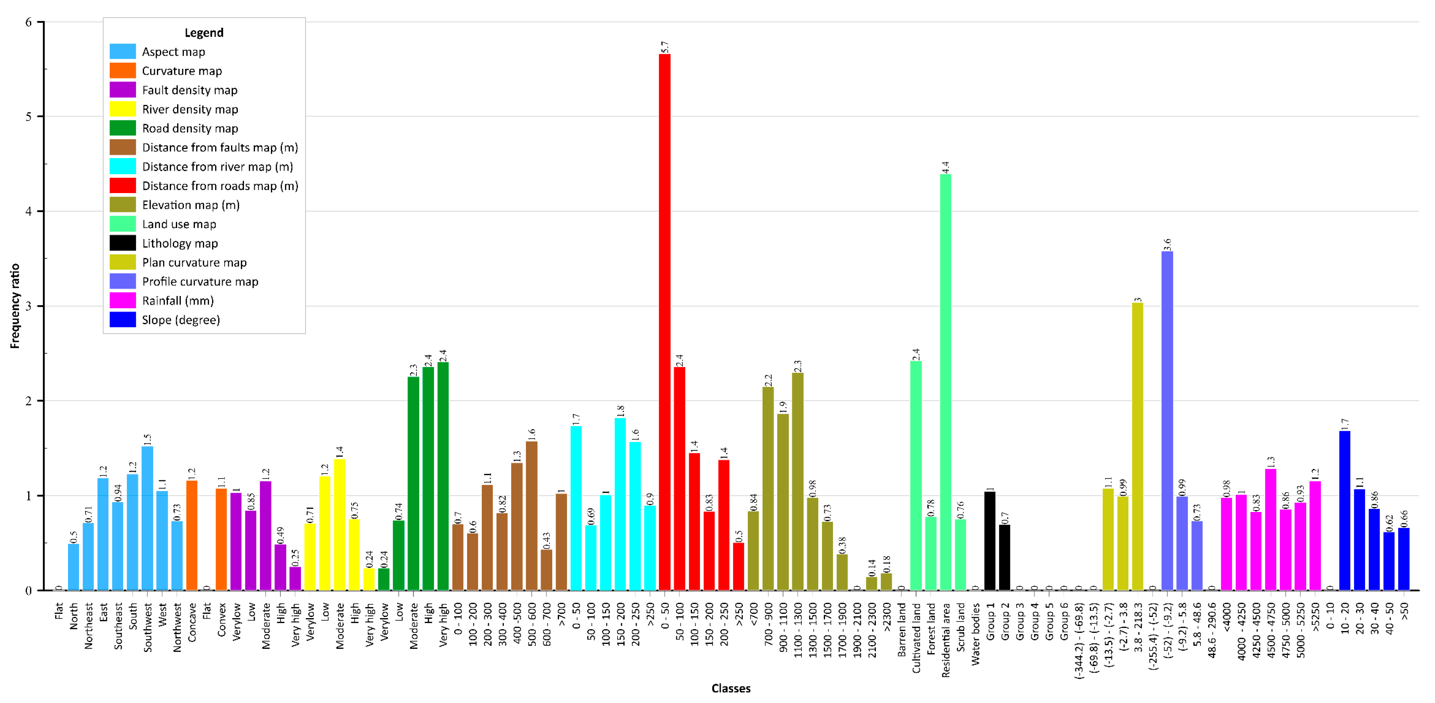
4.1. Important Factors for Landslide Susceptibility Mapping

Table 1. Importance of the conditioning factors using LSVM feature selection method.

No	Factors	Average Merit (AM)	Standard Deviation (SD)
1	Road density	14.7	±0.64
2	Lithology	13.7	±0.458
3	Distance to roads	12.9	±1.64
4	Distance to faults	11.1	±1.375
5	Elevation	10.9	±1.446
6	Plan curvature	9.1	±2.211
7	Fault density	8.3	±2.052
8	Profile curvature	7.7	±2.100
9	Distance to rivers	7.2	±3.450
10	Slope	6.6	±2.010
11	Aspect	5.8	±1.833
12	Curvature	3.4	±1.625
13	Land use	3.2	±1.778
14	Rainfall	3.1	±1.758
15	River density	2.3	±1.418

shows average merit (AM) and standard deviation (SD) metrics of factor selection and also determine the order of significance of each of the conditioning factors using the LSVM technique on landslide susceptibility modeling by the training dataset. AM is a criterion to state the role of each factor on landslide occurrence. A higher value of AM for a given factor shows a greater significant factor for landslide incidence in the modelling process [4,24]. Results indicate that although all factors are important factors in the present study, but a road density with an AM of 14.7 is the most important factor for landslide incidence in this area as the construction of roads creates more instability in the groundmass/rock mass. It is followed by lithology (AM = 13.7), distance to roads (AM = 12.9), distance to faults (AM = 11.1), elevation (AM = 10.9), plan curvature (AM = 9.1), fault density (AM = 8.3), profile curvature (AM = 7.7), distance to river (AM = 7.2), slope (AM = 6.6), aspect (AM = 5.8), curvature (AM = 3.4), land use (AM = 3.2), rainfall (AM = 3.1), and river density (AM = 2.3). However, rainfall has an AM value 3.1, but it is one of the most important triggering factors of landslides. Similarly, erosion and scouring processes are caused by the action of rivers, especially during monsoons. Therefore, all 15 factors, even though they may not have higher AM values, contribute to the occurrence of landslides, and were considered in the present landslide susceptibility modeling.

4.2. Model Construction

Landslide model of SMOSVM was constructed using training dataset generated from the selected factors. Basically, selection of the complexity parameter (C > 0) affects performance of the SMOSVM model [66]. Therefore, the complexity parameter is needed to set up to obtain the highest predictive capability of the SMOSVM model. Krawiec and Bhanu [91] and Kibriya et al. [92] suggested to set the complexity parameter to 10, however, Kurokawa et al. [93] set the complexity parameter equals to 1. In general, no agreement has reached in selection of the certain complexity parameter. In the present study, trial-and-error process [41] was applied to optimize the value of the complexity parameter. The AUC value was utilized to evaluate performance of the SMOSVM model with various values of the complexity parameter. The value of the complexity parameter corresponding to the highest AUC value is selected to build the SMOSVM model. The performance of the SMOSVM model with various values of the complexity parameter is shown in Figure 6. It can be observed that the SMOSVO model has the highest AUC value with the complexity parameter of 7. Therefore, the complexity parameter is set to 7 for training the SMOSVM model in this study. The same value of the complexity parameter was also applied for training individual SVM model and CGSVM. In addition, 10 iterations were used to train the CGSVM.

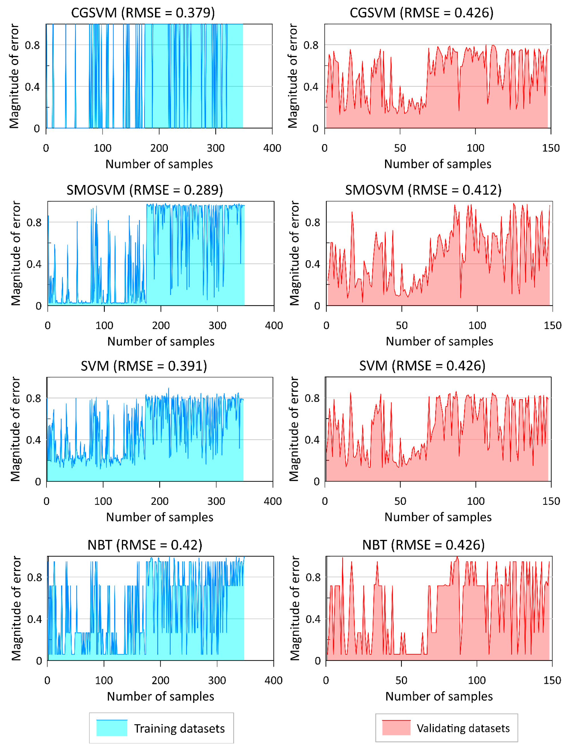
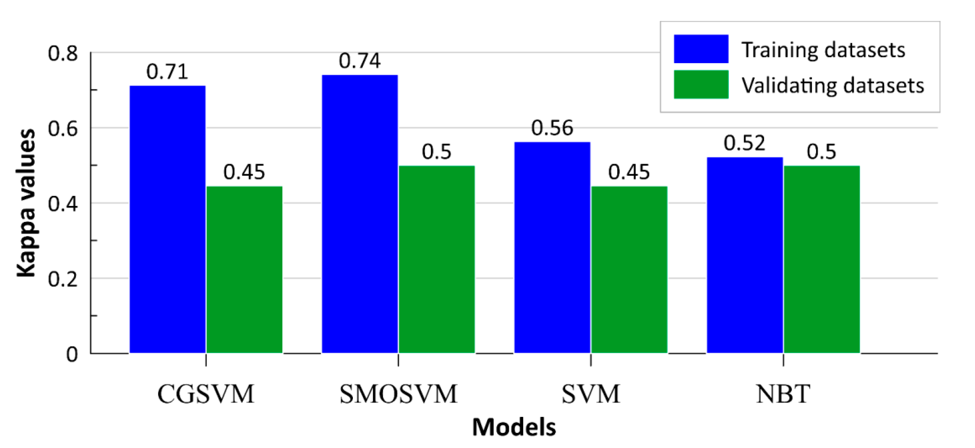
4.3. Model Validation and Comparison

The landslide model of SMOSVM was validated using training (goodness-of-fit) and testing (performance) datasets and different quantitative/statistical metrics. Results of training and testing datasets are shown in Figure 7, Figure 8 and Figure 9. The training results (Figure 7a) indicate that the highest PPV (%) metric was obtained for the CGSVM (88.50%) model, followed by SMOSVM (86.8%), SVM (79.30%), and NBT (77.01%). In terms of NPV (%), SMOSVM has the highest value (87.40%) in comparison to other models including CGSVM (82.80%), SVM (77.00%), and NBT (77.29%). According to SST metric, the result states that SMOSVM (87.30%) is more powerful than CGSVM (83.78%), SVM (77.50%), and NBT (75.71%). However, result indicates that the value of SPF for CGSVM (87.80%) is more than other models, followed by SMOSVM (86.90%), SVM (78.80%), and NBT (76.61%). ACC result illustrates that SMOSVM has the highest value (87.10%) in comparison to other models including CGSVM (85.60%), SVM (78.20%), and NBT (76.15%). Figure 7b shows the results of validation process by testing dataset which is based on PPV values, CGSVM has the highest value of PPV (79.57%), followed by SMOSVM (75.87%), NBT (79.73%), and SVM (74.30%). In terms of NPV, result dedicates that SMOSVM has the highest value (74.30%) in comparison to other models including SVM (70.30%), NBT (70.27%) and CGSVM (64.69%). The result of the SST values for the testing dataset concludes that SMOSVM has the highest value (74.70%), followed by NBT (72.84%), SVM (71.40%), and CGSVM (69.40%). In addition, the results of model validation by SPF depict that NBT has the highest value (77.61%) in comparison to other models including CGSVM (76.20%), SMOSVM (75.30%), and SVM (73.20%). Eventually, results based on ACC and testing detest observe that SMOSVM has the highest value in comparison to other models including SVM, CGSVM, and NBT.

Regarding to RSME values of training (0.289) and validation (0.412) datasets (Figure 8), SMOSVM has the highest goodness-of-fit and performance compared with other landslide models such as CGSVM (RMSE_training = 0.379 and RMSE_validation = 0.426), SVM (RMSE_training = 0.391 and RMSE_validation = 0.426), and NBT (RMSE_training = 0.420 and RMSE_validation = 0.426). In addition to the above-mentioned statistical metrics, the kappa index also was used for model validation and comparison using training and validating detests (Figure 9). Results show that based on the training detest, the kappa value for SMOSVM (0.74) is the highest value. It is followed by CGSVM (0.71), SVM (0.56), and NBT (0.52), respectively. However, using validating dataset results show that SMOSVM (0.5) has the highest value of kappa compared with other models.

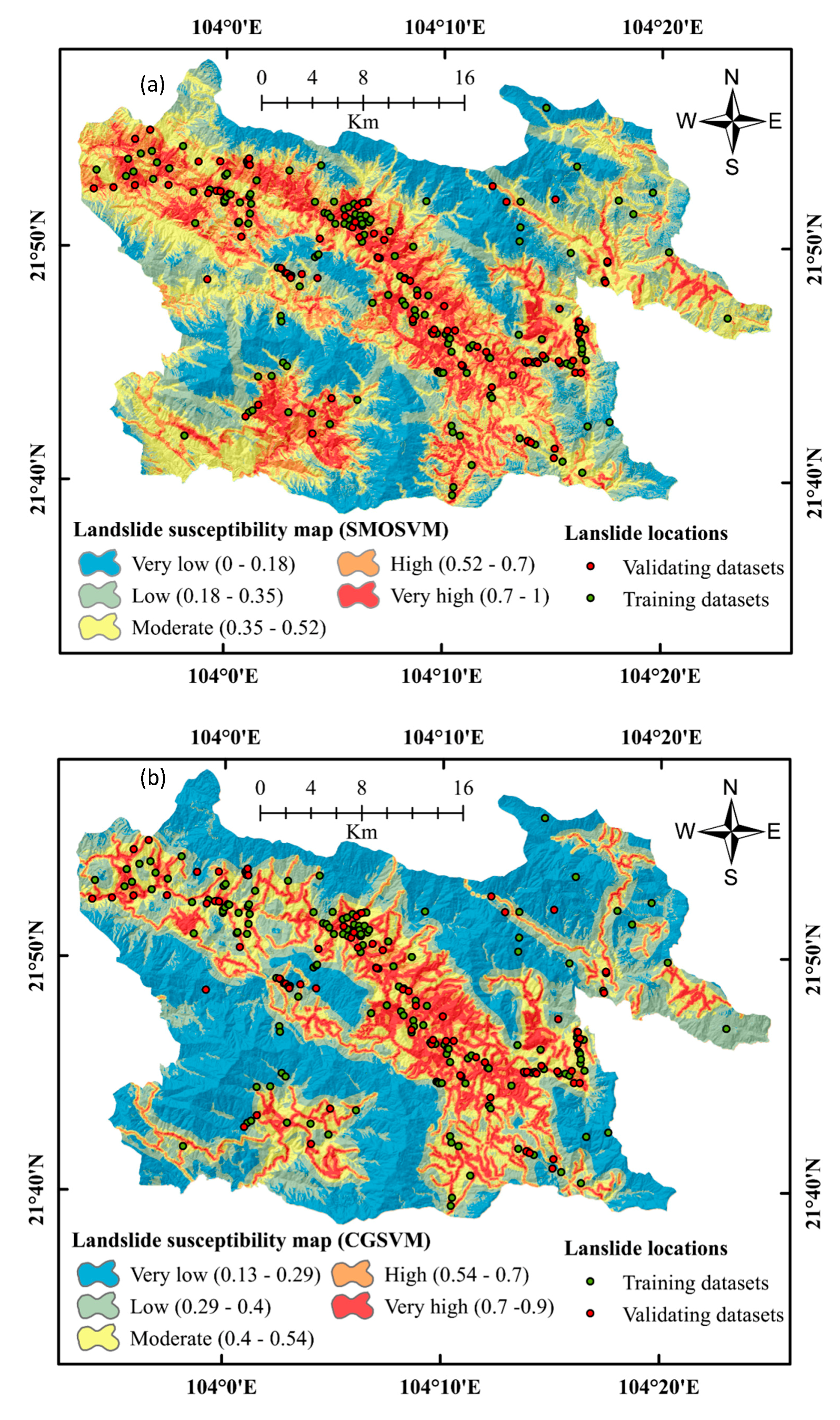
4.4. Development of Landslide Susceptibility Maps

Landslide susceptibility maps of the study area were constructed using analysis of results of the SMOSVM, CGSVM, SVM, and NBT models. Geometrical Intervals (GI) method [94] was used to reclassify landslide susceptibility indexes to make different susceptible classes of all susceptibility maps such as very low, low, high, and very high (Figure 10). For example, in SMOSVM, these classes belonged to (0.004–0.122), (0.122–0.183), (0.183–0.301), (0.301–0.534), and (0.534–0.990), respectively (Figure 10a). Reliability of these maps was evaluated by correlating with the past landslide locations by overlay analysis (Figure 11). It can be pointed out that in SMOSVM moderate class has the highest number of pixels (26.1%), followed by very low and low (22%), high (17.3%), and very high (12.5%), respectively. Moreover, largest numbers of landslide pixels were observed in very high class (86.7%), followed by high and moderate (5.24%), low (2.02%), and very low (0.806%), respectively. In CGSVM, the class of very low susceptibility was assigned most (highest) value of pixels (40.8%) while the lowest one was obtained for the high (10.8%) and very high (11.2%) susceptibility classes. In this model, the highest landslide pixels were obtained for the very high susceptibility class (45.6%), followed by the moderate (16.1%), low (14.9%), high (14.1%), and very low (9.27%) classes. In term of SVM, results conclude that very high class has the highest number of pixels (23.4%), followed by low (21.9%), very low (21.4%), high (17.8%) and moderate (15.4), respectively. However, the largest numbers of landslide pixels were observed in very high class (69.4%), followed by high (13.7%), moderate (8.87%), low (6.85%), and very low (1.21%), respectively. In NBT, value of 36.5% as the highest pixel value was assigned for the moderate class, followed by low (30.8%), high (21.4%), very high (7.2%), and very low (4.19%). Moreover, value of 44% was assigned for very high susceptibility class. It is followed by high (30.2%), moderate (20.2%), low (5.65%), and very low (0%), respectively (Figure 11). Results of analysis show that landslide susceptibility maps produced by these models are reliable as the number of landslide pixels progressively increased from very low susceptibility to very high susceptibility classes. However, the map produced by the proposed SMOSVM model is the most reliable in comparison to other models.

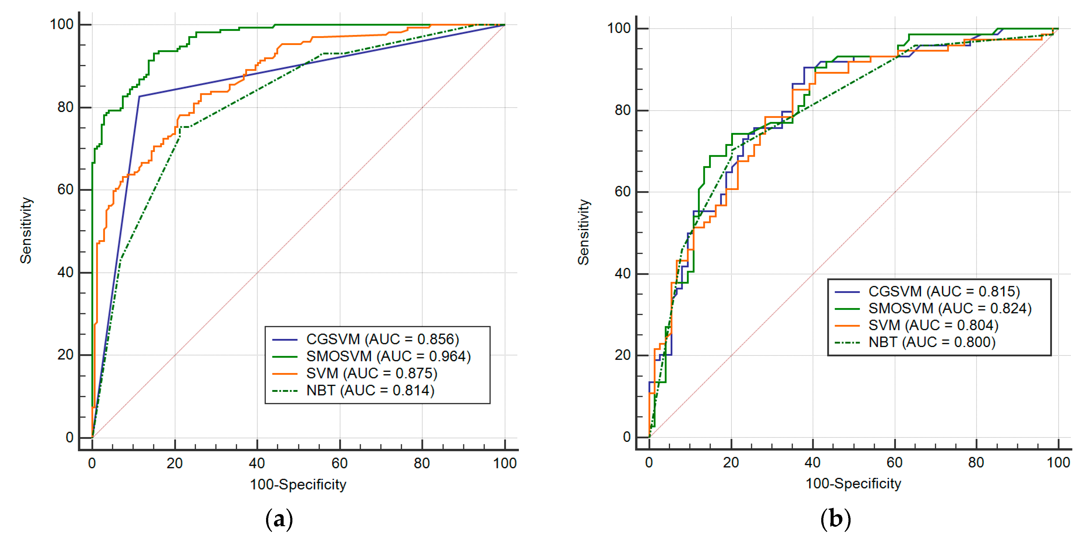
4.5. Evaluation of Landslide Susceptibility Maps

To assess prediction performance of the models and accuracy of produced maps, ROC curve and FR analysis were used. Results of the graphical analysis (Figure 12) illustrate that the SMOSVM model has the highest value of AUC for both training dataset (0.964) and testing dataset (0.824), followed by CGSVM (0.856 and 0.815), SVM (0.875 and 0.804), and NBT (0.814 and 0.800), respectively.

Figure 13 shows FR analysis for the landslide susceptibility maps. The values of FR in the SMOSVM model for very low, low, moderate, high, and very high susceptibility classes are 0.036, 0.091, 0.201, 0.302, and 6.95, respectively. In CGSVM, these values are 0.227, 0.64, 1.17, 1.31, and 4.05, respectively. The most (highest) value of FR was acquired for the very high susceptibility classes (2.96) in SVM, followed by high (0.769), moderate (0.577), low (0.313), and very low (0.056) classes. Finally, the values of FR in NBT for very low, low, moderate, high and very high susceptibility classes are 0, 0.183, 0.553, 1.42, and 6.1, respectively. This study indicates that the FR values from very low to very high susceptibility classes progressively increased; which imply that all landslide models are reliable and have good performance.

5. Discussion

Landslides are one of the most devastating natural hazards in hilly regions all over the world. Progressively, landslide models are being developed using statistical methods and ML techniques to accurately predict landslides for timely taking preventive and protective measures [95]. With this objective, we developed a novel hybrid model SMOSVM to predict accurately landslide occurrences at the Mu Cang Chai District, of Yen Bai Province, Viet Nam. For this, we applied the LSVM technique using a 10-fold cross validation method to select the most important landslide affecting factors. Model studies reveal that although all conditioning factors have positive roles on landslide incidence, road density with the highest average merit (14.7) is more significant for landslide modeling, followed by lithology and distance to roads. In this study, river density was observed the least effective factor. In other areas also factors related to roads are most important in land slide occurrences [14,21,62,95,96]. Main reason is that excavation of roads creates instability of hill slopes by the removal of toe supports and exposes weak geological features/planes on the slope face. This make the road sections vulnerable to slides and sometimes causes landslides at the time of road construction itself.

In the present study, ML and optimization algorithms were used in landslide prediction models as these techniques overcome over-fitting and noise problems. These techniques also have the higher goodness-of-fit and performance in comparison to other conventional models. Moreover, ML ensemble models and optimization algorithms are more powerful and flexible than the individual conventional and machine learning classifiers [33]. Considering the advantage of these models, a novel ensemble intelligence approach, namely SMOSVM, was adopted for landslide susceptibility mapping. For comparison and validation of the proposed model CGSVM, SVM, and NBT algorithms were used. Results indicate that SMOSVM outperforms and outclasses other models, such as CGSVM, SVM, and NBT, using both training (goodness-of-fit) and testing (performance) datasets.

In general, it can be stated that all landslide models perform well in the present study but the SMOSVM model has the highest predictive power for landslide prediction, followed by CGSVM, SVM, and NBT, respectively. It was also observed that performance of the hybrid model SMOSVM model significantly improved in comparison to single by 2% as per analysis of the ROC method. These findings are reasonable as SMOSVM used SMO technique to solve effectively quadratic programming problems. These techniques enhance not only the speed of the SVM model but also the predictive power of the model as it can decrease the over-fitting and noise problems in training dataset [39]. Predictive performance of SMOSVM was evaluated with standard models, such as SVM, which is known as one of the best classifiers for landslide prediction [14]. Another hybrid model, namely NBT, which is a hybrid approach of the naïve Bayes classifier [41] and decision tree classifier [97] is also an efficient method for landslide assessment; however, its performance might be affected by the independent assumption of naïve Bayes classifier [98]. As predictive capability of the SMOSVM model depends on the suitable selection of the complexity parameter (Figure 6) its proper optimization was needed to achieve the best and reliable performance of this model. In the present study, based on the trial-and-error technique [41], the complexity parameter was set to 7 to gain the highest performance of the SMOSVM model.

6. Conclusions

The main objective of the study was to apply a novel hybrid ML model named SMOSVM, which is a combination of SMO and SVM for accurate mapping of landslide susceptibility at the Mu Cang Chai District, Yen Bai Province of Vietnam. SVM is known as a benchmark single model and as one of the powerful classifier, but has a disadvantage in solving large scale quadratic programming, whereas the SMO algorithm overcame the limitations of SVM as SMO has several advantages, such as (i) being a simple and fast training algorithm and being easy to implement; (ii) it can be more successful when the data is large and inputs are spares; and (iii) it can decrease the complexity of difficult problems thus can enhance performance of models.

Preparation of landslide susceptibility maps was carried in this study out using two optimization algorithms namely SMOSVM and CGSVM. Performance of the models was evaluated and validated using area under ROC curve (AUC) and standard statistical measures and results were compared with other benchmark landslide models such as SVM and NBT. Analysis of results indicated that although all landslide models performed well, prediction power of SMOSVM (AUC = 0.824) is the best, followed by CGSVM (AUC = 0.815), SVM (AUC = 0.804), and NBT (AUC = 0.800) models, respectively. Therefore, the SMOSVM model can be considered as a promising method for landslide susceptibility assessment. The present study confirmed that that hybrid model in combination of SMO with SVM is more effective in solving the prediction problems. SMOSVM can be used for the landslide prediction and properly management of landslide-prone areas. More studies are required to select best input parameters including geo-mechanical properties of the rock mass/ground mass in the models for further refining the prediction capabilities of ML methods.

References

1. Van Westen, C.J.; Castellanos, E.; Kuriakose, S.L. Spatial data for landslide susceptibility, hazard, and vulnerability assessment: An overview. Eng. Geol. 2008, 102, 112–131. [Google Scholar] [CrossRef]
2. Guzzetti, F. Landslide Hazard and Risk Assessment. Ph.D. Thesis, University of Bonn, Bonn, Germany, 2006. [Google Scholar]
3. Varnes, D.J. Landslide Hazard. Zonation: A Review of Principles and Practice; UNESCO Press: Paris, France, 1984; p. 63. [Google Scholar]
4. Shirzadi, A.; Solaimani, K.; Roshan, M.H.; Kavian, A.; Chapi, K.; Shahabi, H.; Keesstra, S.; Ahmad, B.B.; Bui, D.T. Uncertainties of prediction accuracy in shallow landslide modeling: Sample size and raster resolution. Catena 2019, 178, 172–188. [Google Scholar] [CrossRef]
5. Yalcin, A. GIS-based landslide susceptibility mapping using analytical hierarchy process and bivariate statistics in Ardesen (Turkey): Comparisons of results and confirmations. Catena 2008, 72, 1–12. [Google Scholar] [CrossRef]
6. Shirzadi, A.; Chapi, K.; Shahabi, H.; Solaimani, K.; Kavian, A.; Ahmad, B.B. Rock fall susceptibility assessment along a mountainous road: An evaluation of bivariate statistic, analytical hierarchy process and frequency ratio. Environ. Earth Sci. 2017, 76, 152. [Google Scholar] [CrossRef]
7. Chen, W.; Chai, H.; Sun, X.; Wang, Q.; Ding, X.; Hong, H. A GIS-based comparative study of frequency ratio, statistical index and weights-of-evidence models in landslide susceptibility mapping. Arab. J. Geosci. 2016, 9, 204. [Google Scholar] [CrossRef]
8. Chen, W.; Li, W.; Hou, E.; Zhao, Z.; Deng, N.; Bai, H.; Wang, D. Landslide susceptibility mapping based on GIS and information value model for the Chencang District of Baoji, China. Arab. J. Geosci. 2014, 7, 4499–4511. [Google Scholar] [CrossRef]
9. Chen, Z.; Liang, S.; Ke, Y.; Yang, Z.; Zhao, H. Landslide susceptibility assessment using evidential belief function, certainty factor and frequency ratio model at Baxie River basin, NW China. Geocarto Int. 2019, 34, 348–367. [Google Scholar] [CrossRef]
10. Hong, H.; Chen, W.; Xu, C.; Youssef, A.M.; Pradhan, B.; Tien Bui, D. Rainfall-induced landslide susceptibility assessment at the Chongren area (China) using frequency ratio, certainty factor, and index of entropy. Geocarto Int. 2017, 32, 139–154. [Google Scholar] [CrossRef]
11. Ding, Q.; Chen, W.; Hong, H. Application of frequency ratio, weights of evidence and evidential belief function models in landslide susceptibility mapping. Geocarto Int. 2017, 32, 619–639. [Google Scholar] [CrossRef]
12. Chen, W.; Shahabi, H.; Shirzadi, A.; Hong, H.; Akgun, A.; Tian, Y.; Liu, J.; Zhu, A.-X.; Li, S. Novel hybrid artificial intelligence approach of bivariate statistical-methods-based kernel logistic regression classifier for landslide susceptibility modeling. Bull. Eng. Geol. Environ. 2019, 78, 4397–4419. [Google Scholar] [CrossRef]
13. Zhu, A.-X.; Wang, R.; Qiao, J.; Qin, C.-Z.; Chen, Y.; Liu, J.; Du, F.; Lin, Y.; Zhu, T. An expert knowledge-based approach to landslide susceptibility mapping using GIS and fuzzy logic. Geomorphology 2014, 214, 128–138. [Google Scholar] [CrossRef]
14. Pham, B.T.; Pradhan, B.; Tien Bui, D.; Prakash, I.; Dholakia, M.B. A comparative study of different machine learning methods for landslide susceptibility assessment: A case study of Uttarakhand area (India). Environ. Model. Softw. 2016, 84, 240–250. [Google Scholar] [CrossRef]
15. Marjanović, M.; Kovačević, M.; Bajat, B.; Voženílek, V. Landslide susceptibility assessment using SVM machine learning algorithm. Eng. Geol. 2011, 123, 225–234. [Google Scholar] [CrossRef]
16. Shirzadi, A.; Shahabi, H.; Chapi, K.; Bui, D.T.; Pham, B.T.; Shahedi, K.; Ahmad, B.B. A comparative study between popular statistical and machine learning methods for simulating volume of landslides. Catena 2017, 157, 213–226. [Google Scholar] [CrossRef]
17. Bui, D.T.; Nhat-Duc, H.; Hieu, N.; Xuan-Linh, T. Spatial prediction of shallow landslide using Bat algorithm optimized machine learning approach: A case study in Lang Son Province, Vietnam. Adv. Eng. Inform. 2019, 42, 100978. [Google Scholar] [CrossRef]
18. Khosravi, K.; Pham, B.T.; Chapi, K.; Shirzadi, A.; Shahabi, H.; Revhaug, I.; Prakash, I.; Bui, D.T. A comparative assessment of decision trees algorithms for flash flood susceptibility modeling at Haraz watershed, northern Iran. Sci. Total Environ. 2018, 627, 744–755. [Google Scholar] [CrossRef] [PubMed]
19. Tien Bui, D.; Shahabi, H.; Shirzadi, A.; Chapi, K.; Alizadeh, M.; Chen, W.; Mohammadi, A.; Ahmad, B.; Panahi, M.; Hong, H. Landslide detection and susceptibility mapping by airsar data using support vector machine and index of entropy models in cameron highlands, malaysia. Remote Sens. 2018, 10, 1527. [Google Scholar] [CrossRef]
20. Shirzadi, A.; Saro, L.; Joo, O.H.; Chapi, K. A GIS-based logistic regression model in rock-fall susceptibility mapping along a mountainous road: Salavat Abad case study, Kurdistan, Iran. Nat. Hazards 2012, 64, 1639–1656. [Google Scholar] [CrossRef]
21. Pham, B.T.; Bui, D.T.; Pourghasemi, H.R.; Indra, P.; Dholakia, M. Landslide susceptibility assesssment in the Uttarakhand area (India) using GIS: A comparison study of prediction capability of naïve bayes, multilayer perceptron neural networks, and functional trees methods. Theor. Appl. Climatol. 2017, 128, 255–273. [Google Scholar] [CrossRef]
22. Chen, W.; Pourghasemi, H.R.; Naghibi, S.A. A comparative study of landslide susceptibility maps produced using support vector machine with different kernel functions and entropy data mining models in China. Bull. Eng. Geol. Environ. 2018, 77, 647–664. [Google Scholar] [CrossRef]
23. Tien Bui, D.; Shahabi, H.; Shirzadi, A.; Chapi, K.; Pradhan, B.; Chen, W.; Khosravi, K.; Panahi, M.; Bin Ahmad, B.; Saro, L. Land subsidence susceptibility mapping in south korea using machine learning algorithms. Sensors 2018, 18, 2464. [Google Scholar] [CrossRef] [PubMed]
24. Shirzadi, A.; Soliamani, K.; Habibnejhad, M.; Kavian, A.; Chapi, K.; Shahabi, H.; Chen, W.; Khosravi, K.; Thai Pham, B.; Pradhan, B. Novel GIS based machine learning algorithms for shallow landslide susceptibility mapping. Sensors 2018, 18, 3777. [Google Scholar] [CrossRef] [PubMed]
25. Chen, W.; Shahabi, H.; Shirzadi, A.; Li, T.; Guo, C.; Hong, H.; Li, W.; Pan, D.; Hui, J.; Ma, M. A novel ensemble approach of bivariate statistical-based logistic model tree classifier for landslide susceptibility assessment. Geocarto Int. 2018, 33, 1398–1420. [Google Scholar] [CrossRef]
26. Shirzadi, A.; Bui, D.T.; Pham, B.T.; Solaimani, K.; Chapi, K.; Kavian, A.; Shahabi, H.; Revhaug, I. Shallow landslide susceptibility assessment using a novel hybrid intelligence approach. Environ. Earth Sci. 2017, 76, 60. [Google Scholar] [CrossRef]
27. Abedini, M.; Ghasemian, B.; Shirzadi, A.; Shahabi, H.; Chapi, K.; Pham, B.T.; Bin Ahmad, B.; Tien Bui, D. A novel hybrid approach of bayesian logistic regression and its ensembles for landslide susceptibility assessment. Geocarto Int. 2018, 1–31. [Google Scholar] [CrossRef]
28. Chapi, K.; Singh, V.P.; Shirzadi, A.; Shahabi, H.; Bui, D.T.; Pham, B.T.; Khosravi, K. A novel hybrid artificial intelligence approach for flood susceptibility assessment. Environ. Model. Softw. 2017, 95, 229–245. [Google Scholar] [CrossRef]
29. Hong, H.; Panahi, M.; Shirzadi, A.; Ma, T.; Liu, J.; Zhu, A.-X.; Chen, W.; Kougias, I.; Kazakis, N. Flood susceptibility assessment in Hengfeng area coupling adaptive neuro-fuzzy inference system with genetic algorithm and differential evolution. Sci. Total Environ. 2018, 621, 1124–1141. [Google Scholar] [CrossRef] [PubMed]
30. Tien Bui, D.; Khosravi, K.; Li, S.; Shahabi, H.; Panahi, M.; Singh, V.; Chapi, K.; Shirzadi, A.; Panahi, S.; Chen, W. New hybrids of anfis with several optimization algorithms for flood susceptibility modeling. Water 2018, 10, 1210. [Google Scholar] [CrossRef]
31. Ahmadlou, M.; Karimi, M.; Alizadeh, S.; Shirzadi, A.; Parvinnejhad, D.; Shahabi, H.; Panahi, M. Flood susceptibility assessment using integration of adaptive network-based fuzzy inference system (ANFIS) and biogeography-based optimization (BBO) BAT algorithms (BA). Geocarto Int. 2019, 34, 1252–1272. [Google Scholar] [CrossRef]
32. Tien Bui, D.; Shahabi, H.; Shirzadi, A.; Chapi, K.; Hoang, N.-D.; Pham, B.; Bui, Q.-T.; Tran, C.-T.; Panahi, M.; Bin Ahamd, B. A novel integrated approach of relevance vector machine optimized by imperialist competitive algorithm for spatial modeling of shallow landslides. Remote Sens. 2018, 10, 1538. [Google Scholar] [CrossRef]
33. Pham, B.T.; Shirzadi, A.; Bui, D.T.; Prakash, I.; Dholakia, M. A hybrid machine learning ensemble approach based on a radial basis function neural network and rotation forest for landslide susceptibility modeling: A case study in the Himalayan area, India. Int. J. Sediment. Res. 2018, 33, 157–170. [Google Scholar] [CrossRef]
34. Kavzoglu, T.; Sahin, E.K.; Colkesen, I. Landslide susceptibility mapping using GIS-based multi-criteria decision analysis, support vector machines, and logistic regression. Landslides 2014, 11, 425–439. [Google Scholar] [CrossRef]
35. Pourghasemi, H.R.; Jirandeh, A.G.; Pradhan, B.; Xu, C.; Gokceoglu, C. Landslide susceptibility mapping using support vector machine and GIS at the Golestan Province, Iran. J. Earth Syst. Sci. 2013, 2, 349–369. [Google Scholar] [CrossRef] [Green Version]
36. Yao, X.; Tham, L.G.; Dai, F.C. Landslide susceptibility mapping based on Support Vector Machine: A case study on natural slopes of Hong Kong, China. Geomorphology 2008, 101, 572–582. [Google Scholar] [CrossRef]
37. Lai, K.K.; Yu, L.; Zhou, L.; Wang, S. Credit Risk Evaluation with Least Square Support Vector Machine. In Proceedings of the International Conference on Rough Sets and Knowledge Technology; Springer: Berlin/Heidelberg, Germany, 2006; pp. 490–495. [Google Scholar]
38. Platt, J. Fast training of support vector machines using sequential minimal optimization. In Advances in Kernel Methods Support Vector Learning; Schölkopf, B., Burges, C.J.C., Smola, A.J., Eds.; MIT Press: Cambridge, MA, USA, 1999. [Google Scholar]
39. Gama, J.; Brazdil, P. Cascade generalization. Mach. Learn. 2000, 41, 315–343. [Google Scholar] [CrossRef]
40. Ercanoglu, M.; Gokceoglu, C. Assessment of landslide susceptibility for a landslide-prone area (north of Yenice, NW Turkey) by fuzzy approach. Environ. Geol. 2002, 41, 720–730. [Google Scholar]
41. Bui, D.T.; Hoang, N.D.; Martínez-Álvarez, F.; Ngo, P.T.T.; Hoa, P.V.; Pham, T.D.; Samui, P.; Costache, R. A novel deep learning neural network approach for predicting flash flood susceptibility: A case study at a high frequency tropical storm area. Sci. Total Environ. 2019. [Google Scholar] [CrossRef]
42. Bui, D.T.; Moayedi, H.; Kalantar, B.; Osouli, A.; Pradhan, B.; Nguyen, H.; Rashid, A.S.A. A Novel Swarm Intelligence—Harris Hawks Optimization for Spatial Assessment of Landslide Susceptibility. Sensors 2019, 19, 3590. [Google Scholar] [CrossRef] [PubMed] [Green Version]
43. Tien Bui, D.; Ho, T.-C.; Pradhan, B.; Pham, B.-T.; Nhu, V.-H.; Revhaug, I. GIS-based modeling of rainfall-induced landslides using data mining-based functional trees classifier with AdaBoost, Bagging, and MultiBoost ensemble frameworks. Environ. Earth Sci. 2016, 75, 1–22. [Google Scholar] [CrossRef]
44. Ayalew, L.; Yamagishi, H.; Ugawa, N. Landslide susceptibility mapping using GIS-based weighted linear combination, the case in Tsugawa area of Agano River, Niigata Prefecture, Japan. Landslides 2004, 1, 73–81. [Google Scholar] [CrossRef]
45. Stocking, M. Relief analysis and soil erosion in Rhodesia using multi-variate techniques. Z. Geomorphol. NF 1972, 16, 432–443. [Google Scholar]
46. Pham, B.T.; Tien Bui, D.; Prakash, I.; Dholakia, M.B. Rotation forest fuzzy rule-based classifier ensemble for spatial prediction of landslides using GIS. Nat. Hazards 2016, 83, 1–31. [Google Scholar] [CrossRef]
47. Brewer, C.A. Basic mapping principles for visualizing cancer data using geographic information systems (GIS). Am. J. Prev. Med. 2006, 30, S25–S36. [Google Scholar] [CrossRef] [PubMed]
48. Pradhan, B. Use of GIS-based fuzzy logic relations and its cross application to produce landslide susceptibility maps in three test areas in Malaysia. Environ. Earth Sci. 2011, 63, 329–349. [Google Scholar] [CrossRef]
49. Pradhan, B.; Abokharima, M.H.; Jebur, M.N.; Tehrany, M.S. Land subsidence susceptibility mapping at Kinta Valley (Malaysia) using the evidential belief function model in GIS. Nat. Hazards 2014, 73, 1019–1042. [Google Scholar] [CrossRef]
50. Komac, M. A landslide susceptibility model using the analytical hierarchy process method and multivariate statistics in perialpine Slovenia. Geomorphology 2006, 74, 17–28. [Google Scholar] [CrossRef]
51. Pradhan, B.; Lee, S. Landslide susceptibility assessment and factor effect analysis: Backpropagation artificial neural networks and their comparison with frequency ratio and bivariate logistic regression modelling. Environ. Model. Softw. 2010, 25, 747–759. [Google Scholar] [CrossRef]
52. Ercanoglu, M.; Gokceoglu, C.; Van Asch, T.W. Landslide susceptibility zoning north of Yenice (NW Turkey) by multivariate statistical techniques. Nat. Hazards 2004, 32, 1–23. [Google Scholar] [CrossRef]
53. Ohlmacher, G.C.; Davis, J.C. Using multiple logistic regression and GIS technology to predict landslide hazard in northeast Kansas, USA. Eng. Geol. 2003, 69, 331–343. [Google Scholar] [CrossRef]
54. Pham, B.T.; Tien Bui, D.; Indra, P.; Dholakia, M.B. Landslide susceptibility assessment at a part of Uttarakhand Himalaya, India using GIS—Based statistical approach of frequency ratio method. Int. J. Eng. Res. Technol. 2015, 4, 338–344. [Google Scholar]
55. Tien Bui, D.; Pradhan, B.; Lofman, O.; Revhaug, I.; Dick, O.B. Landslide susceptibility mapping at Hoa Binh province (Vietnam) using an adaptive neuro-fuzzy inference system and GIS. Comput. Geosci. 2012, 45, 199–211. [Google Scholar] [CrossRef]
56. Tien Bui, D.; Pradhan, B.; Lofman, O.; Revhaug, I.; Dick, O.B. Landslide susceptibility assessment in the Hoa Binh province of Vietnam: A comparison of the Levenberg–Marquardt and Bayesian regularized neural networks. Geomorphology 2012, 171, 12–29. [Google Scholar] [CrossRef]
57. Pham, B.T.; Nguyen, M.D.; Le, A.H. Shear resistance and stability study of embankments using different shear resistance parameters of soft soils from laboratory and field tests: A case study of Hai Phong city, Viet Nam. Int. J. Sci. Res. Dev. 2016, 3, 330–334. [Google Scholar]
58. NCEP. Global Weather Data for SWAT. 2014. Available online: http://globalweather.tamu.edu/home (accessed on 15 March 2017).
59. Ayalew, L.; Yamagishi, H. The application of GIS-based logistic regression for landslide susceptibility mapping in the Kakuda-Yahiko Mountains, Central Japan. Geomorphology 2005, 65, 15–31. [Google Scholar] [CrossRef]
60. Van, T.T.; Anh, D.T.; Hieu, H.H.; Giap, N.X.; Ke, T.D.; Nam, T.D.; Ngoc, D.; Ngoc, D.T.Y.; Thai, T.N.; Thang, D.V.; et al. Investigation and Assessment of the Current Status and Potential of Landslides in Some Sections of the Ho Chi Minh Road, National Road 1A and Proposed Remedial Measures to Prevent Landslides from Threat of Safety of People, Property, and Infrastructure; Vietnam Institute of Geosciences and Mineral Resources: Hanoi, Vietnam, 2006; p. 249. [Google Scholar]
61. Tien Bui, D. Modeling of Rainfall-Induced Landslide Hazard for the Hoa Binh Province of Vietnam. Ph.D. Thesis, Norwegian University of Life Sciences, Aas, Norway, 2012. [Google Scholar]
62. Nguyen, P.T.; Tuyen, T.T.; Shirzadi, A.; Pham, B.T.; Shahabi, H.; Omidvar, E.; Amini, A.; Entezami, H.; Prakash, I.; Phong, T.V. Development of a novel hybrid intelligence approach for landslide spatial prediction. Appl. Sci. 2019, 9, 2824. [Google Scholar] [CrossRef] [Green Version]
63. Arora, M.; Das Gupta†, A.; Gupta, R. An artificial neural network approach for landslide hazard zonation in the Bhagirathi (Ganga) Valley, Himalayas. Int. J. Remote Sens. 2004, 25, 559–572. [Google Scholar] [CrossRef]
64. Vapnik, V. The Nature of Statistical Learning Theory; Springer: Berlin/Heidelberg, Germany, 1995. [Google Scholar]
65. Vapnik, V.N.; Vapnik, V. Statistical Learning Theory; Wiley: New York, NJ, USA, 1998; Volume 1. [Google Scholar]
66. Gulyani, B.B.; Mangai, J.A.; Fathima, A. An Approach for Predicting River Water Quality Using Data Mining Technique. In Advances in Data Mining: Applications and Theoretical Aspects; Springer: Berlin/Heidelberg, Germany, 2015; pp. 233–243. [Google Scholar]
67. Suykens, J.A.; Vandewalle, J. Least squares support vector machine classifiers. Neural Process. Lett. 1999, 9, 293–300. [Google Scholar] [CrossRef]
68. Bonansea, L. 3D Hand gesture recognition using a ZCam and an SVM-SMO classifier. Master’s Thesis, Iowa State University, Ames, IA, USA, 2009. [Google Scholar]
69. Nugroho, K.A.; Setiawan, N.A.; Adji, T.B. Cascade Generalization for Breast Cancer Detection. In Proceedings of the 2013 International Conference on Information Technology and Electrical Engineering (ICITEE), Yogyakarta, Indonesia, 7–8 October 2013; pp. 57–61. [Google Scholar]
70. Kotsiantis, S.; Kanellopoulos, D. Cascade Generalization with Classification and Model Trees. In Proceedings of the 2008 Third International Conference on Convergence and Hybrid Information Technology, Busan, Korea, 11–13 November 2008; pp. 248–253. [Google Scholar]
71. Zhao, H.; Ram, S. Entity matching across heterogeneous data sources: An approach based on constrained cascade generalization. Data Knowl. Eng. 2008, 66, 368–381. [Google Scholar] [CrossRef]
72. Ludwig, O.; Nunes, U.; Ribeiro, B.; Premebida, C. Improving the Generalization Capacity of Cascade Classifiers. IEEE Trans. Cybern. 2013, 43, 2135–2146. [Google Scholar] [CrossRef] [PubMed]
73. Barakat, N. Cascade generalization: Is SVMs’ inductive bias useful? In Proceedings of the 2010 IEEE International Conference on Systems, Man and Cybernetics, Istanbul, Turkey, 10–13 October 2010; pp. 1393–1399. [Google Scholar]
74. Wolpert, D.H. Stacked generalization. Neural Netw. 1992, 5, 241–259. [Google Scholar] [CrossRef]
75. Chen, W.; Xie, X.; Peng, J.; Wang, J.; Duan, Z.; Hong, H. GIS-based landslide susceptibility modelling: A comparative assessment of kernel logistic regression, Naïve-Bayes tree, and alternating decision tree models. Geomat. Nat. Hazards Risk 2017, 8, 950–973. [Google Scholar] [CrossRef] [Green Version]
76. Chen, W.; Zhang, S.; Li, R.; Shahabi, H. Performance evaluation of the GIS-based data mining techniques of best-first decision tree, random forest, and naïve Bayes tree for landslide susceptibility modeling. Sci. Total Environ. 2018, 644, 1006–1018. [Google Scholar] [CrossRef] [PubMed]
77. Pham, B.T.; Prakash, I. A novel hybrid model of Bagging-based Naïve Bayes Trees for landslide susceptibility assessment. Bull. Eng. Geol. Environ. 2017. [Google Scholar] [CrossRef]
78. Quinlan, J.R. Induction of Decision Trees. Mach. Learn. 1986, 1, 81–106. [Google Scholar] [CrossRef] [Green Version]
79. Chen, W.; Hong, H.; Li, S.; Shahabi, H.; Wang, Y.; Wang, X.; Ahmad, B.B. Flood susceptibility modelling using novel hybrid approach of reduced-error pruning trees with bagging and random subspace ensembles. J. Hydrol. 2019, 575, 864–873. [Google Scholar] [CrossRef]
80. Bennett, N.D.; Croke, B.F.; Guariso, G.; Guillaume, J.H.; Hamilton, S.H.; Jakeman, A.J.; Marsili-Libelli, S.; Newham, L.T.; Norton, J.P.; Perrin, C. Characterising performance of environmental models. Environ. Model. Softw. 2013, 40, 1–20. [Google Scholar] [CrossRef]
81. Abedini, M.; Ghasemian, B.; Shirzadi, A.; Bui, D.T. A comparative study of support vector machine and logistic model tree classifiers for shallow landslide susceptibility modeling. Environ. Earth Sci. 2019, 78, 560. [Google Scholar] [CrossRef]
82. Tien Bui, D.; Shirzadi, A.; Shahabi, H.; Geertsema, M.; Omidvar, E.; Clague, J.J.; Thai Pham, B.; Dou, J.; Talebpour Asl, D.; Bin Ahmad, B. New Ensemble Models for Shallow Landslide Susceptibility Modeling in a Semi-Arid Watershed. Forests 2019, 10, 743. [Google Scholar] [CrossRef] [Green Version]
83. Chen, W.; Tsangaratos, P.; Ilia, I.; Duan, Z.; Chen, X. Groundwater spring potential mapping using population-based evolutionary algorithms and data mining methods. Sci. Total Environ. 2019, 684, 31–49. [Google Scholar] [CrossRef] [PubMed]
84. Chen, W.; Hong, H.; Panahi, M.; Shahabi, H.; Wang, Y.; Shirzadi, A.; Pirasteh, S.; Alesheikh, A.A.; Khosravi, K.; Panahi, S. Spatial Prediction of Landslide Susceptibility Using GIS-Based Data Mining Techniques of ANFIS with Whale Optimization Algorithm (WOA) and Grey Wolf Optimizer (GWO). Appl. Sci. 2019, 9, 3755. [Google Scholar] [CrossRef] [Green Version]
85. Chen, W.; Panahi, M.; Khosravi, K.; Pourghasemi, H.R.; Rezaie, F.; Parvinnezhad, D. Spatial prediction of groundwater potentiality using ANFIS ensembled with teaching-learning-based and biogeography-based optimization. J. Hydrol. 2019, 572, 435–448. [Google Scholar] [CrossRef]
86. Pham, B.T.; Prakash, I.; Dou, J.; Singh, S.K.; Trinh, P.T.; Tran, H.T.; Le, T.M.; Van Phong, T.; Khoi, D.K.; Shirzadi, A. A novel hybrid approach of landslide susceptibility modelling using rotation forest ensemble and different base classifiers. Geocarto Int. 2019. [Google Scholar] [CrossRef]
87. Chen, W.; Pradhan, B.; Li, S.; Shahabi, H.; Rizeei, H.M.; Hou, E.; Wang, S. Novel hybrid integration approach of bagging-based fisher’s linear discriminant function for groundwater potential analysis. Nat. Resour. Res. 2019, 28, 1239–1258. [Google Scholar] [CrossRef] [Green Version]
88. Chen, W.; Shahabi, H.; Zhang, S.; Khosravi, K.; Shirzadi, A.; Chapi, K.; Pham, B.T.; Zhang, T.; Zhang, L.; Chai, H.; et al. Landslide Susceptibility Modeling Based on GIS and Novel Bagging-Based Kernel Logistic Regression. Appl. Sci. 2018, 8, 2540. [Google Scholar] [CrossRef] [Green Version]
89. Rahmati, O.; Falah, F.; Dayal, K.; Deo, R.C.; Mohammadi, F.; Biggs, T.; Moghaddam, D.D.; Naghibi, S.A.; Tien Bui, D. Machine learning approaches for spatial modeling of agricultural droughts in south-east region of Queensland Australia. Sci. Total Environ. 2019. [Google Scholar] [CrossRef] [PubMed]
90. Chen, W.; Xie, X.; Wang, J.; Pradhan, B.; Hong, H.; Tien Bui, D.; Duan, Z.; Ma, J. A comparative study of logistic model tree, random forest, and classification and regression tree models for spatial prediction of landslide susceptibility. Catena 2017, 151, 147–160. [Google Scholar] [CrossRef] [Green Version]
91. Krawiec, K.; Bhanu, B. Coevolution and linear genetic programming for visual learning. In Genetic and Evolutionary Computation—GECCO 2003; Springer: Berlin/Heidelberg, Germany, 2003; pp. 332–343. [Google Scholar]
92. Kibriya, A.M.; Frank, E.; Pfahringer, B.; Holmes, G. Multinomial naive bayes for text categorization revisited. In AI 2004: Advances in Artificial Intelligence; Springer: Berlin/Heidelberg, Germany, 2005; pp. 488–499. [Google Scholar]
93. Kurokawa, M.; Yokoyama, H.; Sakurai, A. Averaged Naive Bayes Trees: A New Extension of AODE. In Advances in Machine Learning; Springer: Berlin/Heidelberg, Germany, 2009; pp. 191–205. [Google Scholar]
94. Frye, C. About the Geometrical Interval Classification Method. 2007. Available online: http://blogs.esri.com/esri/arcgis (accessed on 15 April 2018).
95. Tien Bui, D.; Shahabi, H.; Omidvar, E.; Shirzadi, A.; Geertsema, M.; Clague, J.J.; Khosravi, K.; Pradhan, B.; Pham, B.T.; Chapi, K. Shallow landslide prediction using a novel hybrid functional machine learning algorithm. Remote Sens. 2019, 11, 931. [Google Scholar] [CrossRef] [Green Version]
96. Pham, B.T.; Bui, D.T.; Prakash, I.; Dholakia, M. Hybrid integration of Multilayer Perceptron Neural Networks and machine learning ensembles for landslide susceptibility assessment at Himalayan area (India) using GIS. Catena 2017, 149, 52–63. [Google Scholar] [CrossRef]
97. Zhao, Y.; Zhang, Y. Comparison of decision tree methods for finding active objects. Adv. Space Res. 2008, 41, 1955–1959. [Google Scholar] [CrossRef] [Green Version]
98. Pham, B.T.; Bui, D.T.; Prakash, I.; Dholakia, M. Evaluation of predictive ability of support vector machines and naive Bayes trees methods for spatial prediction of landslides in Uttarakhand state (India) using GIS. J. Geomat. 2016, 10, 71–79. [Google Scholar]
Figure 1. Landslide training and testing locations of the study area.
Sustainability 11 06323 g001
Figure 2. Landslide photos from Yen Bai Province (source: VIGMR).
Sustainability 11 06323 g002
Figure 3. Landslide affective factors: (a) aspect, (b) curvature, (c) fault density, (d) distance to faults, (e) river density, (f) distance to rivers, (g) road density, (h) distance to roads, (i) slope, (j) rainfall, (k) profile curvature, (l) plan curvature, (m) lithology, (n) land use, and (o) elevation [62].
Sustainability 11 06323 g003aSustainability 11 06323 g003b
Figure 4. Analysis of frequency ratio of factor maps [62].
Sustainability 11 06323 g004
Figure 5. Methodological flowchart of the study.
Sustainability 11 06323 g005
Figure 6. Performance of the SMOSVM model with various values of the complexity parameter.
Sustainability 11 06323 g006
Figure 7. Values of PPV, NPV, SST, SPF, and ACC of the models: (a) training dataset and (b) testing dataset.
Sustainability 11 06323 g007
Figure 8. Error analysis of the models using training and testing datasets.
Sustainability 11 06323 g008
Figure 9. Value of kappa of the models using training dataset and testing datasets.
Sustainability 11 06323 g009
Figure 10. Landslide susceptibility maps of the study area using various models: (a) SMOSVM, (b) CGSVM, (c) SVM, and (d) NBT.
Sustainability 11 06323 g010aSustainability 11 06323 g010b
Figure 11. Histogram of class and landslide pixels on landslide susceptibility maps.
Sustainability 11 06323 g011
Figure 12. Analysis of the ROC curve of the SMOSVM landslide model: (a) using the training dataset, (b) using the testing dataset.
Sustainability 11 06323 g012
Figure 13. Analysis of FR of the susceptibility maps of the models.
Sustainability 11 06323 g013