Air Pollutant Emissions from Vehicles and Their Abatement Scenarios: A Case Study of Chengdu-Chongqing Urban Agglomeration, China

Abstract

Vehicular emissions have become one of the important sources of air pollution, and their effective control is essential to protect the environment. The Chengdu-Chongqing Urban Agglomeration (CCUA), a less developed area located in the southwest of China with higher vehicle population and special topographic features, was selected as the research area. The aims of this study were to establish multi-year vehicular emission inventories for ten important air pollutants in this area and to analyze emission control policy scenarios based on the inventories. The results showed that the ten vehicular pollutant emissions had differences during the past decade, and CO₂ and NH₃ increased markedly between 1999 and 2015. Chengdu and Chongqing were the dominant contributors of vehicular emissions in the CCUA. Eight scenarios based on these inventories were designed and the alternative energy replacement scenario was studied from the life-cycle perspective. Compared with the business as usual scenario, elimination of substandard vehicles scenario is the most effective policy to control NO_x, PM_2.5, PM₁₀, and CH₄ emissions; the radical alternative energy replacement scenario could decrease the vehicular NMVOC, CO₂, N₂O, and NH₃ emissions; the elimination of motorcycles scenario could decrease the vehicular CO emissions; and the raising fuel standards scenario could reduce vehicular SO₂ emissions significantly (by 94.81%). The radical integrated scenario (combining all of the reduction control measures mentioned above) would achieve the maximum emission reduction of vehicular pollutants CO, NMVOC, NO_x, PM_2.5, PM₁₀, CO₂, N₂O, and NH₃ compared with any scenario alone.

1. Introduction

As the hazy weather increases, many parts of China (such as the Beijing-Tianjin-Hebei Region, Yangtze River Delta, Pearl River Delta, and Chengdu-Chongqing Urban Agglomeration (CCUA)) are suffering from serious air pollution [1,2]. Previous research showed that carbon dioxide emissions and other air pollutants are positively related to the economic development of countries [3], meaning that the rapid economic development will bring more pollutants if not controlled in the future. With the rapid development of economics in China, the vehicle population is undergoing a sharp growth. The vehicle population in China increased from 14.53 million in 1999 to 162.84 million in 2015 which increased more than 11 times in seventeen years [4] (Figure 1). Subsequently, the rapid increase in vehicle population has brought a large number of pollutants emissions. In China, the vehicles emitted 45.32 million of tons of pollutants in 2015, including 5.8 million of tons of nitrogen oxides (NO_x), 560,000 tons of particulate matters (PM), 4.3 million tons of hydrocarbons (HC), and 34.6 million of tons of carbon monoxide (CO) [5]. Vehicular emissions have become the predominant source of air pollution in China [6] and can have direct or indirect adverse effects on human health [7]. Such as, particulate matter (PM) emitted by vehicles could directly increase atmospheric particulate matter with a diameter less than 2.5 µm (PM_2.5) [7], which can harm human health and reduce the life quality of residents. There is, thus, an urgent need to study regional vehicular emissions and emission reduction strategies in China.

Many studies research on the vehicular emissions estimation and control strategies using different methods for some areas [8,9,10]. In China, Che (2010) studied the vehicular pollutant reduction control strategy and evaluated the emission reduction effects of five control measures, including “eliminating the yellow label vehicle (eliminating gasoline vehicles where emission level is lower than the State I emission standard, and diesel vehicles where emission level is lower than the State III emission standard in China)” and “implementing new emission standards” in the Pearl River Delta region. Tian (2013) [11] used the COPERT model to establish vehicular emission inventory for Nanjing in 2011, then proposed four emission reduction scenarios (including single and double number limits and wrong time peaks), and analyzed the emission reductions of the scenarios. Li (2015) [12] estimated vehicular emission inventory (CO, NO_x, HC, and PM) for the Beijing-Tianjin-Hebei region between 2007 and 2011 based on COPERT model and analyzed its emission characteristics, then set up five reduction scenarios and assessed their emission reductions effects. Guo et al. (2016) [13] used the scenario analysis method to estimate vehicular emissions of CO, NO_x, hydrocarbons, and PM₁₀ in Beijing for 2011–2020 for three pollutant control measures. However, as researchers have paid more attention to vehicular emissions on the developed regions and cities of China, few studies have focused on the vehicular emissions and emission reduction strategies of the Chinese central and western regions, such as the CCUA. In addition, the evaluation on emission reduction effects of the existing studies was not comprehensive enough as they lacked the life-cycle analysis of the new energy vehicles under various emission reduction measures.

In recent years, the vehicle population in the CCUA has increased continuously along with the rapid development of the economy of this area under the strong support of national policies. As the two largest cities in the CCUA, the vehicle population of Chongqing and Chengdu were next only to Beijing and ranked second and third in China in recent years. The disharmonious status that vehicle population has grown much faster than the local economy has appeared in these cities. The potential environmental threat will be greater. In addition, when confronted with adverse climate and geography conditions, the emission mitigation in this region will be harder to achieve and the environmental governance will be more difficult than in other regions. In addition, the special basin terrain in this area also increases the pollutant emission and is not conducive to the diffusion of pollutants. The CCUA is also the important platform of Chinese western development, the strategic support for the Yangtze River economic belt, and an important demonstration area for promoting new urbanization (Figure 2). Thus, there is a need to study the characteristics of vehicular pollutant emission and emission reduction strategies in this area for its particularity.

The purposes of this study are to investigate a multi-pollutant vehicular emissions inventory including both conventional pollutants and greenhouse gases between 1999 and 2015 and analyze its trends and characteristics, and to assess the emission reduction effect of different control measures in the CCUA. Vehicular emission trends were analyzed to ensure the integrity of the regional pollutant emission inventory. The vehicular emission results were used to define eight pollutant emission reduction scenarios (including business as usual (BAU), high standard replacement (HSR), raising fuel standards (RFS), elimination of substandard vehicles (ESV), public transport priority (PTP), alternative energy replacement (AER), elimination of motorcycles (EMC), and integrated scenario (IS)), and the effects of implementing these scenarios were estimated. A radical alternative energy replacement (RAER) scenario was evaluated using life-cycle evaluation.

2. Methodology

The methodology section includes two parts. In Section 2.1, we introduce the vehicular emissions estimates including data sources and prediction methods of vehicle population, vehicle kilometers travelled (VKT), and emission factors. In Section 2.2, we design the reduction scenarios based on the emission inventory. Figure 3 shows the method system construction.

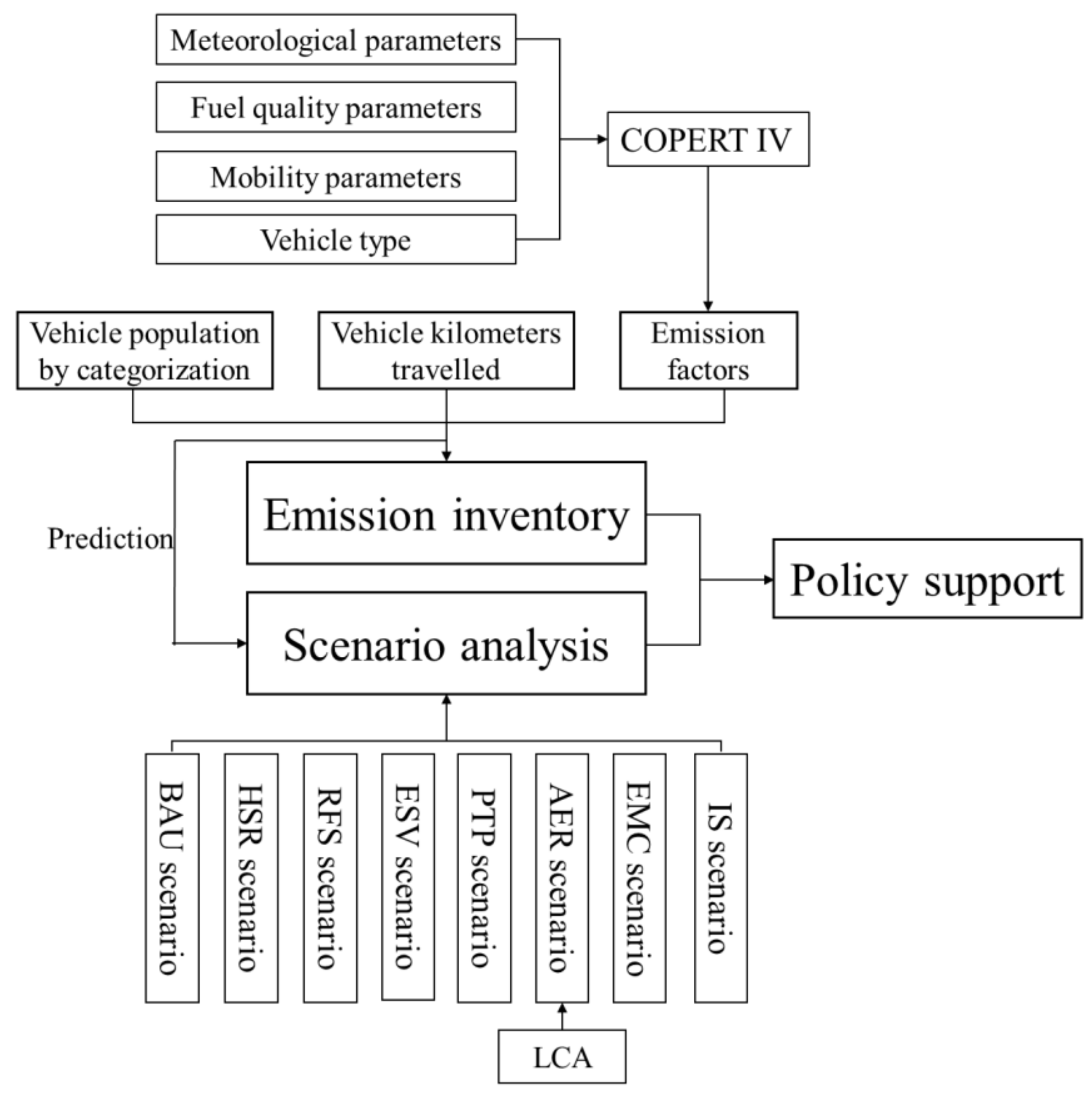
2.1. Emission Estimates

Vehicular emissions were calculated from the vehicle populations, annual mean vehicle kilometers travelled (VKT) and emission factors using Equation (1),

$${\mathrm{Q}}_{\mathrm{m},\mathrm{n}}={\displaystyle \sum }_{\mathrm{i}}{\displaystyle \sum }_{\mathrm{j}}\left({\mathrm{P}}_{\mathrm{m},\mathrm{i},\mathrm{j}}\times {\mathrm{VKT}}_{\mathrm{m},\mathrm{i}}\times {\mathrm{EF}}_{\mathrm{i},\mathrm{j},\mathrm{n}}\right)$$

(1)

where Q_m,n is the amount of pollutant n emitted in area m each year, P_m,i,j is the number of vehicles in category i with emission standard j in area m, VKT_m,i is the mean annual VKT (km) for vehicles in category i in area m, and EF_i,j,_n is the emission factor (g/km) for pollutant n emitted by vehicles in category i with emission standard j. In this study, m represents 16 cities in the CCUA. The vehicle categories in this work include passenger car (PC), bus (BUS), light-duty vehicle (LDV), heavy-duty truck (HDT), and motorcycle (MC).

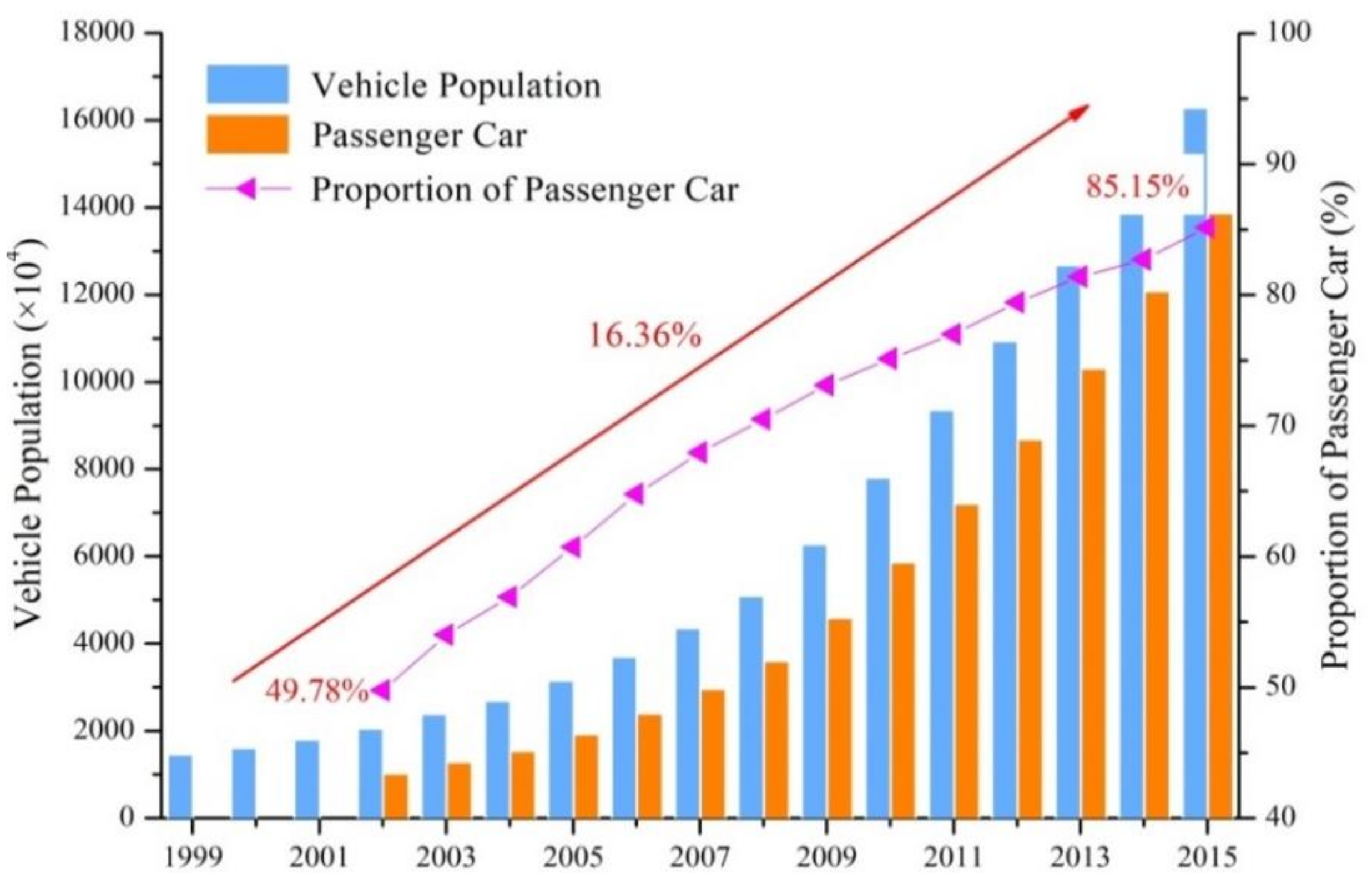
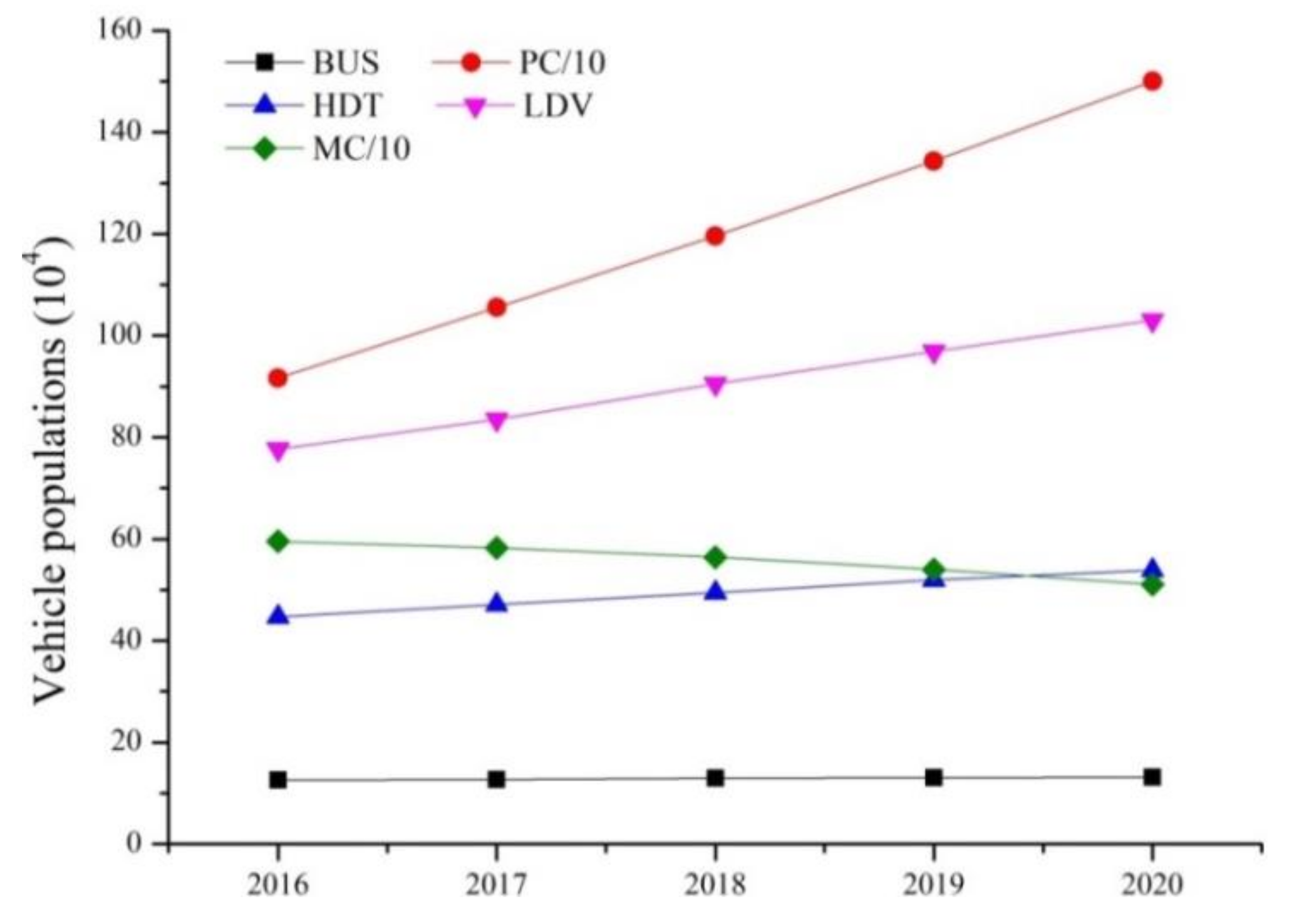
2.1.1. Vehicle Population

The vehicle populations of each vehicle category in each city in the CCUA between 1999 and 2015 were obtained from the official statistical yearbooks [4,14,15,16] and statistical bulletins for national economic and social development of each city. New vehicles must follow any new standard once it has been implemented [17,18]. The dates of introduction of new vehicular emission standards in the CCUA are summarized in Table S1. The vehicle populations which the emission standards for the different vehicle types were implemented were calculated using the annual numbers of new vehicle registrations, vehicle survival rates, and the dates of implementation of the vehicular emission standards in the different cities using the method of our previous study [19].

The categorical prediction method was used to predict the vehicle population of each city in the CCUA between 2016 and 2020. The PC population was affected by many factors, particularly per capita income. Numerous studies [20,21] have demonstrated that the PC population conforms to the Gompertz model curve, i.e., the vehicle retention rate increases with per capita income and follows an S-shaped curve. The vehicle retention rate increases to a maximum and then decreases until it reaches a plateau. The PC population was predicted using the Gompertz function,

$$\mathrm{V}\left(\mathrm{x}\right)=\mathsf{\gamma }{e}^{{\alpha }^{e^{\left(\beta x\right)}}}$$

(2)

where V(x) represents the PC population (units/thousand people), x is the per capita disposable income (yuan/person), γ is the PC retention rate plateau (values obtained from publications by Ji et al. (2013) [22] and Guo et al. (2016) [13], and a value of 0.4 was selected), and α and β are parameters indicating the model trend, obtained by fitting a line to a plot of the PC retention rate data (the PC population divided by the demographic data) for 1999–2015 against per capita disposable income. The per capita disposable incomes for 16 cities (for 2016–2020) were projected from equivalent incomes from 1999–2015. The PC population retention rates for each city for 2016–2020 were predicted using Equation (2). The populations of the cities in 2016–2020 were predicted using the GM (1, 1) grey model. The PC populations of the cities in 2016–2020 were calculated from these data. The HDT, LDV, BUS, and MC populations were predicted using the regression curve method. The CCUA vehicle populations in 2016–2020 (shown in Figure 4) were then calculated. The same method was used to predict the population of newly registered vehicles in each city for 2016–2020. The future age distributions for each vehicle type were calculated according to the vehicle survival rates [19], assuming that each vehicle met the relevant emission standard in the registration year. Therefore, the vehicle populations implementing different emission standards in each city from 2016 to 2020 were determined.

2.1.2. Vehicle Kilometers Travelled (VKT)

The mean annual VKT, a major vehicle activity level indicator, can influence vehicular emissions. VKT data for different vehicle types were not available because VKT data are not included in official statistical records. VKT data for the CCUA were obtained from previous studies [23,24,25,26,27,28,29,30], and referred to the research on the annual VKT data of cities with a similar level of economic development and vehicle population, given that both the VKT values and vehicle population are strongly related to economic activity [28,31,32]. The missing data were obtained from linear interpolations [1].

The average annual VKT values for different vehicle types in cities in the CCUA between 2016 and 2020 were predicted. It was previously found that the average annual VKT for PC correlates with its retention rate [32], i.e., the annual VKT decreases as the retention rate increases each year. The PC retention rate in a city is expected to continue to grow. An index correlation between the annual PC VKT and retention rate for each city was therefore established using the annual VKT of PC for each city in the CCUA from 1999 to 2015. The annual VKT of PC from 2016 to 2020 was determined from the PC retention rates for 2016–2020, as predicted using the Gompertz curve. The annual VKT values of HDT, BUS, and LDV are related to commercial activities and increase with economic growth. Therefore, annual VKT values of HDT, LDV, and BUS for 2016–2020 were predicted using the elasticity coefficient method. The elastic coefficients for the annual average growth rate of VKT of HDT, LDV, and BUS, and annual GDP growth rates for 1999–2015 were calculated. The annual average growth rate of GDP for each city for 2016–2020 was predicted from relevant predictions of potential GDP growth rates made by the Chinese Academy of Social Sciences. The annual VKT values of HDT, LDV, and BUS for 2016–2020 were then calculated. The annual VKT of MC will decrease in the next few years because motorcycle use limits are being applied in each city. The predicted annual VKT values of different vehicle types are summarized in Table S2.

2.1.3. Emission Factors

The Computer Programme to calculate Emissions from Road Transport (COPERT) Ⅳ (v11.2) model was used to estimate vehicular emission factors. The main parameters used in the COPERT Ⅳ model include vehicle population, mean driving speed, fuel quality, and meteorological data. The vehicle types used in the model are different from the Chinese vehicle types. The method used to convert between the two types is shown in Table S3. The mean driving speeds for the different vehicle types were obtained from existing researches [1,23,24,29,33,34]. Fuel quality parameters were obtained from Chinese national and local fuel standards. The gasoline and diesel sulfur contents are summarized in Table S4. Meteorological data referred to the Chinese Meteorological Yearbook [35].

Emission factor for the different vehicle types in different cities were predicted using the COPERT IV model using predicted values for the parameters as required by the model. The predicted parameters included fuel consumption, temperature, and humidity, etc. Gasoline and diesel consumption were predicted using the linear regression method. There is no ideal method for predicting temperature and humidity for short periods on a monthly basis. The predicted maximum temperature, minimum temperature, and mean humidity each month between 2016 and 2020, were defined as the mean maximum temperature, minimum temperature, and mean humidity, respectively, in the same months between 1999 and 2015. These predictions and the results of previous studies [36,37,38,39] allowed vehicle pollutant emission factors for 2016–2020 to be estimated.

2.2. Design of Reduction Scenarios

2.2.1. BAU Scenario

The BAU scenario involved the use of existing vehicular emissions control measures, the natural elimination of vehicles, and not implementing any additional emission reduction measures.

2.2.2. HSR Scenario

The HSR scenario is defined in terms of the application of higher emission standards to new vehicles to meet vehicular pollutant emission standards set by the Chinese Ministry of Environmental Production and the CCUA in future (

Table 1. Vehicular emission standards implementation timetable.

Vehicle Type	State V	State VI
PC, LDV	20170101	/
	20180101
BUS, HDT	20170101	/
	20170701

). Other control measures were the same as in the BAU scenario.

2.2.3. RFS Scenario

Implementing new oil quality standards could cause an immediate decrease in vehicular emissions. Decreasing the sulfur content of vehicle fuel is essential to decrease vehicular emission sulfur. The sulfur contents of oil products were predicted from the plans made by each city to implement vehicle oil standards. The RFS scenario was set according to the fuel quality that the CCUA may implement in the future (

Table 2. Vehicular fuel standards implementation timetable.

Fuel Type	State V	State VI
Gasoline	2017	2019
Diesel	2017	2019

). The vehicle population and annual VKT were the same as for the BAU scenario. Emission factors were determined using the RFS parameters in the COPERT IV model.

2.2.4. ESV Scenario

Elimination of yellow-label vehicles and heavily-polluting vehicles will effectively decrease vehicular pollutant emissions. The ESV scenario is shown in

Table 3. Timetable of elimination of substandard vehicles.

2015	2017	2018	2020
/	Yellow-label vehicles Pre-State-I MC	/	Gasoline State-I and State-II vehicles Diesel State-III vehicles State-I and State-II MC

. The emission factors and annual VKT values were the same as for the BAU scenario. The total number of vehicles was maintained by assuming all the eliminated vehicles were replaced with vehicles meeting up-to-date emission standards in the year the vehicles were replaced.

2.2.5. PTP Scenario

The development of public transport is an effective means of increasing the proportion of residents using public transport and decreasing the number of PC and MC used, thus decreasing the mean PC and MC VKT. It was previously found that the annual PC VKT decreases by 1% per year as the proportion of public transportation used increased [40]. We assumed that limiting MC use would decrease the mean MC VKT by 2% per year. The PTP scenario implies that PC and MC VKT in 2020 will be 5% and 15% lower than the baseline for the CCUA, respectively.

2.2.6. AER Scenario

The promotion of vehicles using new energy sources is an effective means to decrease energy consumption and pollutant emissions. However, a large proportion of the electricity in China is produced by coal-powered plants. Decreases in pollutant emissions achieved through the promotion of electric vehicles are substantially reduced if the upstream pollutant emissions are considered. Life-cycle assessment methods must be used to assess electric vehicles. We therefore used a conservative alternative energy replacement (CAER) scenario and a radical alternative energy replacement (RAER) scenario to assess emission reductions achieved using electric and hybrid vehicles, and vehicles powered by natural gas (

Table 4. The description of alternative energy replacement scenario.

Scenarios	Scenario Setting
CAER	90% of BUS using alternative fuels and advanced vehicle power technologies by 2020, among which, electric, hybrids, and natural-gas powered BUS would account for 10%, 10%, and 80%, respectively;PC powered by natural gas, hybrid, and electric would account for 20%, 5%, and 5% by 2020
RAER	The electricity provided to the vehicles would be produced using “clean” energy. The other RAER parameters were the same as for the CAER scenario.

).

Emission factors for hybrid and natural-gas vehicles were referred from the existing research [36,37,38,39,41,42,43] (Table S5). The annual hybrid and natural-gas vehicles VKT values were the same as for the BAU scenario. These data allowed the estimation of emissions from hybrid and natural-gas vehicles in the CCUA.

The life-cycle of an electric vehicle was analyzed using the Greenhouse Gases, Regulated Emissions, and Energy Use in Transportation (GREET) model developed by the National Argonne Laboratory and used in previous existing studies [44,45,46]. The electric vehicle life-cycle includes the fuel and material life-cycles. The fuel life-cycle has two phases, the well-to-tank phase and the tank-to-wheels phase, which covers raw material production, fuel supply, and driving. Energy consumption, greenhouse gas emissions, and pollutant emissions during the fuel life-cycle account for 70–90% of the total life-cycle. The material life-cycle accounts for a relatively small proportion of the total life-cycle. It was difficult to obtain energy consumption and pollutant emission data for the material life-cycle because numerous materials are processed and used when manufacturing vehicles. Therefore, the study was focused on the electric vehicle fuel life-cycle.

(1)

Calculating energy consumption

Coal-fired power plants are the most important sources of electricity in China. The fuel life- cycle analysis was therefore focused on pollutants emitted by coal-fired power plants. The Chinese power industry has developed rapidly in recent years, and the total power generated has increased each year. Total power generated by the Chinese power industry in 2020 is predicted to be 7.4 trillion kWh [46]. The proportions of power produced by different methods were determined from the national average power composition data. Coal-fired power plants are predicted to contribute 78% of the electricity produced in China in 2020 [47,48], assuming this for the CCUA. Energy consumption and pollutant emissions from power plants are closely related to the power generation efficiency. The International Energy Agency predicted that Chinese coal-fired power plants will have a generation efficiency of 38% in 2020. Assuming this to be the same for the CCUA, as for China as a whole, the power generation efficiency was calculated using the Equation (3):

$$\alpha =\frac{\beta \times \mu }{\gamma \times \pi }$$

(3)

where α is the coal-fired power generation efficiency (%), γ is the amount of standard coal used in coal-fired power plants (kg), π is the low calorific value of standard coal (J/kg), β is the amount of electricity produced by coal-fired power plant (kWh), and µ is the electro-thermal conversion coefficient (J/kWh).

(2)

Calculating pollutant emissions

CO₂ emissions were estimated using the carbon balance method. CO₂ emissions were determined by adding direct CO₂ emissions and indirect CO₂ emissions together. The carbon in direct CO₂ emissions was defined as the amount of carbon in the combustion products (VOC, CO and CH₄) subtracted from the amount of carbon in the raw fuel. Indirect CO₂ emissions were calculated from the VOC and CO emissions [46].

Non-combustion emissions and dust pollution were not taken into account because the study was focused on combustion emissions of CO, NMVOC, NO_x, PM_2.5, PM₁₀, CH₄, N₂O, and SO₂. NH₃ emissions in the upstream stage of the vehicles were excluded because it was very difficult to estimate an NH₃ emission factor. SO₂ emissions were estimated using the sulfur balance method [44]. Emissions of the other pollutants were calculated using Equation (4):

$$N_{WT{T}_I}={\displaystyle \sum }_J{\displaystyle \sum }_{K}E{F}_{i,\mathrm{j},\mathrm{k}}\times M_{j,\mathrm{k}}\times 100$$

(4)

where $N_{WT{T}_I}$ denotes pollutant i emissions during combustion (g/km), $E{F}_{i,j,k}$ is the pollutant i emission factor (kg/kJ), and $M_{j,\mathrm{k}}$ is fuel consumption (kJ/km). $M_{j,\mathrm{k}}$ was calculated using Equation (5):

$$M_{j,k}=M\times P_j\times T_j$$

(5)

where M is fuel consumption (kJ/km), P is the proportion of fuel used, T is the proportion of control technology, i is the pollutant species, j is the fuel type, and k is the type of control technology.

Power plant, boiler combustion emissions, and emissions during transportation are main sources of pollutant emissions in the well-to-tank phase for electric vehicles. The remainder of this section is focused on emissions caused by combustion in power plants and boilers.

Emission factor for power plants was calculated using Equation (6):

$$E{F}_I=E{F}_{I,\mathrm{NC}}\times {\displaystyle \sum }_j\left[W_{i,j}\times \left(1-{\sigma }_{i,j}\right)\right]$$

(6)

where EF_I is the emission factor (g/kWh), EF_I,NC is the emission factor in an uncontrolled state (g/kWh), W_i,j is the control technology application ratio (%), σ_i,j is the pollutant removal efficiency (%), i is the pollutant species, and j is the control technology category.

Relatively small amounts of CO, VOC, CH₄ and N₂O are emitted by thermal power plants in China, therefore measures for controlling these pollutants were not considered. The emission factors used were the default values from the GREET model. Large amounts of SO₂, NO_x, PM_2.5, and PM₁₀ are emitted by thermal power plants in China, and the parameters required for calculating actual emission factors for these pollutants were taken from previous publications [17,48,49,50,51,52].

Emission factors for coal-fired industrial boilers were calculated using the method described above. Relatively small amounts of CO, VOC, CH₄, and N₂O are emitted by coal-fired industrial boilers; thus, measures to control these pollutants were not considered. The VOC, CH₄, and N₂O emission factors were taken from previous publications [44,53]. The default CO emission factor in the GREET model was used. The SO₂, NO_x, PM_2.5, and PM₁₀ emission factors for boilers under uncontrolled state, with efficient removal, and with control technology used were taken from previous publications [54,55,56].

Upstream emissions for individual PC and BUS in the CCUA were estimated using the method described above, as shown in Table S6.

2.2.7. EMC Scenario

In the CCUA, MCs are major contributors of vehicular emissions. The number of MCs eliminated was determined from the urban and suburban population proportions for each city [37]. In the EMC scenario, MCs are assumed to be completely banned in all urban centers in the CCUA by 2020. The other vehicle populations, emission factors, and vehicular emission standard implementation times were the same as for the BAU scenario.

2.2.8. Integrated Scenario

The integrated scenario was divided into a conservative integrated scenario (CIS) and a radical integrated scenario (RIS). The CIS combined all the control measures, and the effects of the emission reduction measures were calculated from the effects of each individual control measures. In the RIS, power for electric vehicles was assumed to be supplied by “clean” energy sources. The other parameters were the same as for the CIS.

3. Results and Discussion

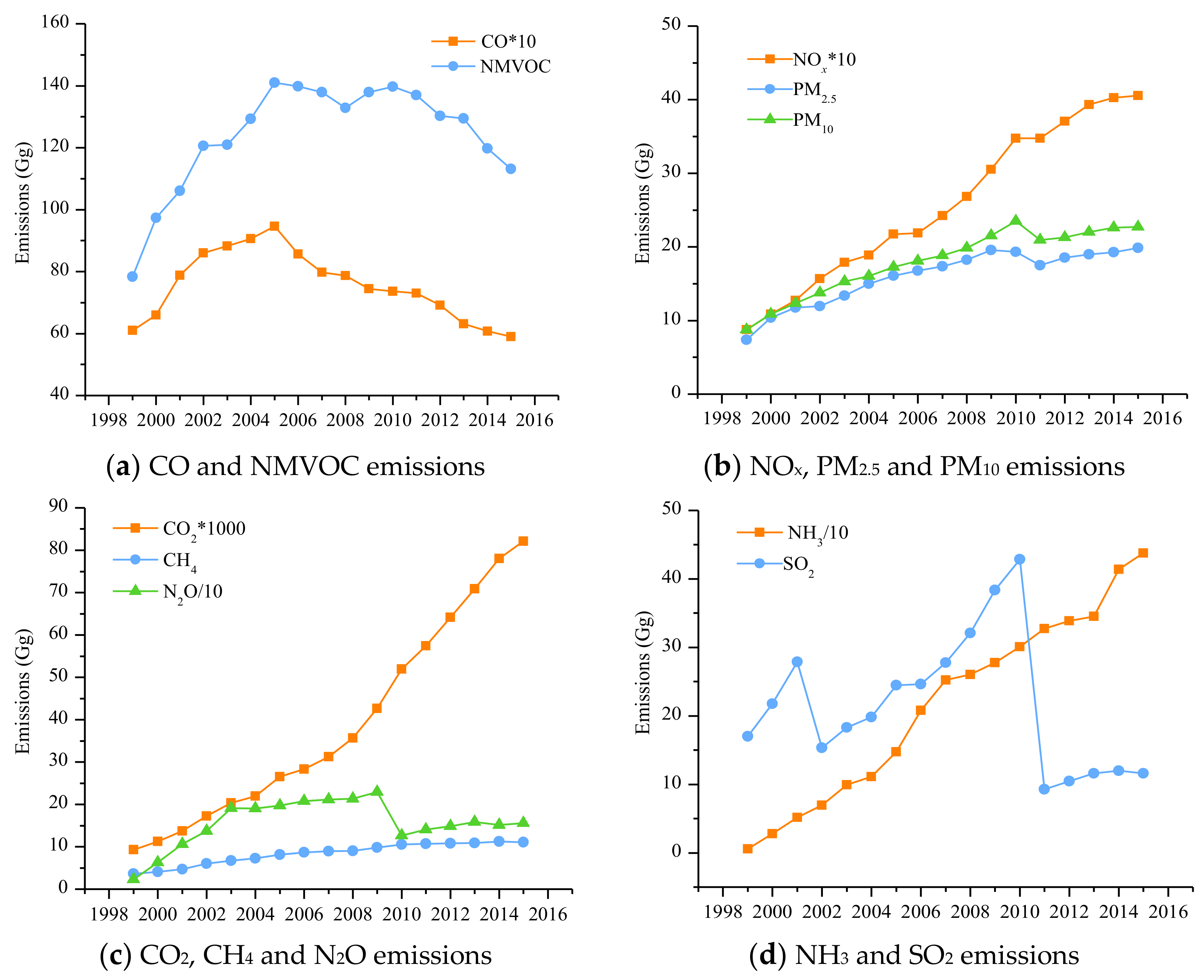
3.1. Vehicular Emission Inter-Annual Trends for Different Pollutants

Vehicular emissions of CO, NMVOC, NO_x, PM_2.5, PM₁₀, CO₂, CH₄, N₂O, NH₃, and SO₂ in the CCUA were calculated based on the methods described in Section 2, and the vehicular emission inter-annual trend for different pollutants are shown in Figure 5.

Vehicular emissions of CO and NMVOC increased each year by (on average) 7.74% and 10.52%, respectively, between 1999 and 2005 in the CCUA. With the stricter emission standards (from State II to State IV, see Table S1) implemented in recent years, vehicular CO and NMVOC emissions decreased from 945.87 Gg and 141.04 Gg, respectively, in 2005, to 589.98 Gg and 113.17 Gg, respectively, in 2015. NO_x, PM_2.5, and PM₁₀ emissions increased between 1999 and 2015. NO_x, PM_2.5, and PM₁₀ emissions in 2015 were 405.78 Gg, 19.87 Gg, and 22.7 Gg, respectively, and these were 362.79%, 169.56%, and 158.98% higher, respectively, than those in 1999.

Vehicular CO₂ emissions changed from 9287.72 Gg in 1999 to 82090.23 Gg in 2015 and increased by 783.86%. This increase indicates that fuel standards implemented in China were not effective in decreasing vehicular CO₂ emissions. Furthermore, the number of PCs increased markedly in China as industrialization and urbanization progressed and living standards improved. PCs were the main contributors to vehicular CO₂ emissions, and the large increases in the numbers of PCs offset decreases in CO₂ emissions by individual PCs caused by the implementation of fuel standards. Vehicular CH₄ emissions increased and then decreased. Total vehicular CH₄ emissions increased from 3.62 Gg in 1999 to 11.27 Gg in 2014, representing an annual increase of 8.08%. This was related to the larger number of natural gas vehicles in the CCUA, which were rich in natural gas resources. CH₄ emissions then decreased to 11.05 Gg in 2015. Vehicular N₂O emissions increased from 0.227 Gg in 1999 to 1.555 Gg in 2015, with an increase of 582.32%. However, N₂O emissions decreased from 2.295 Gg in 2009 to 1.269 Gg in 2010. This was due to new fuel standards, which caused fuel quality to improve (the sulfur content of fuel strongly affects vehicular N₂O emissions). Decreasing the sulfur content of fuel is an important way of decreasing vehicular N₂O emissions [18]. The sulfur content of gasoline decreased from 500 mg/L in 2009 to 150 mg/L in 2010 in the CCUA (Table S4). Vehicular N₂O emissions decreased in some years but mainly followed an upward trend because increases in PC numbers offset decreases in emissions per PC caused by the implementation of fuel standards. There is a clear need to restrict the numbers of PCs to decrease pollutant emissions.

Vehicular NH₃ emissions were found to have increased by more than emissions of the other pollutants. NH₃ emissions increased from 0.056 Gg in 1999 to 4.37 Gg in 2015, with an increase of 7637.72%. Hazy weather in China is mainly caused by PM_2.5 [57]. NH₃ emitted by vehicles is essential to the formation and growth of PM_2.5. NH₃ is an alkaline gas that can react with water and acidic substances (e.g., SO₂ and NO_x) to form major contributors to fine particles (e.g., ammonium sulfate and ammonium nitrate) [58]. Vehicle populations and traffic flows are much higher in city centers than in surrounding areas, and NH₃ promotes hazy weather; therefore, haze is a more serious problem in city centers than in suburbs. The Chinese government, and indeed society in general, has focused very little on attention to NH₃ pollution, and vehicular NH₃ emissions must be decreased. Vehicular SO₂ emissions are mainly controlled by sulfur content in fuels and vehicle population [59]. SO₂ emissions in the CCUA changed in ways different from other pollutants between 1999 and 2015 (Figure 5). This was mainly caused by the specification of different sulfur contents in fuel standards implemented between 1999 and 2015 (Table S4). Vehicular SO₂ emissions increased between 1999 and 2015 except for between 2001 and 2002, and between 2010 and 2011 when SO₂ emissions markedly decreased (from 27.87 Gg in 2001 to 15.34Gg in 2002, and from 42.86 Gg in 2010 to 9.28 Gg in 2011, decreases of 81.67% and 361.99%, respectively).

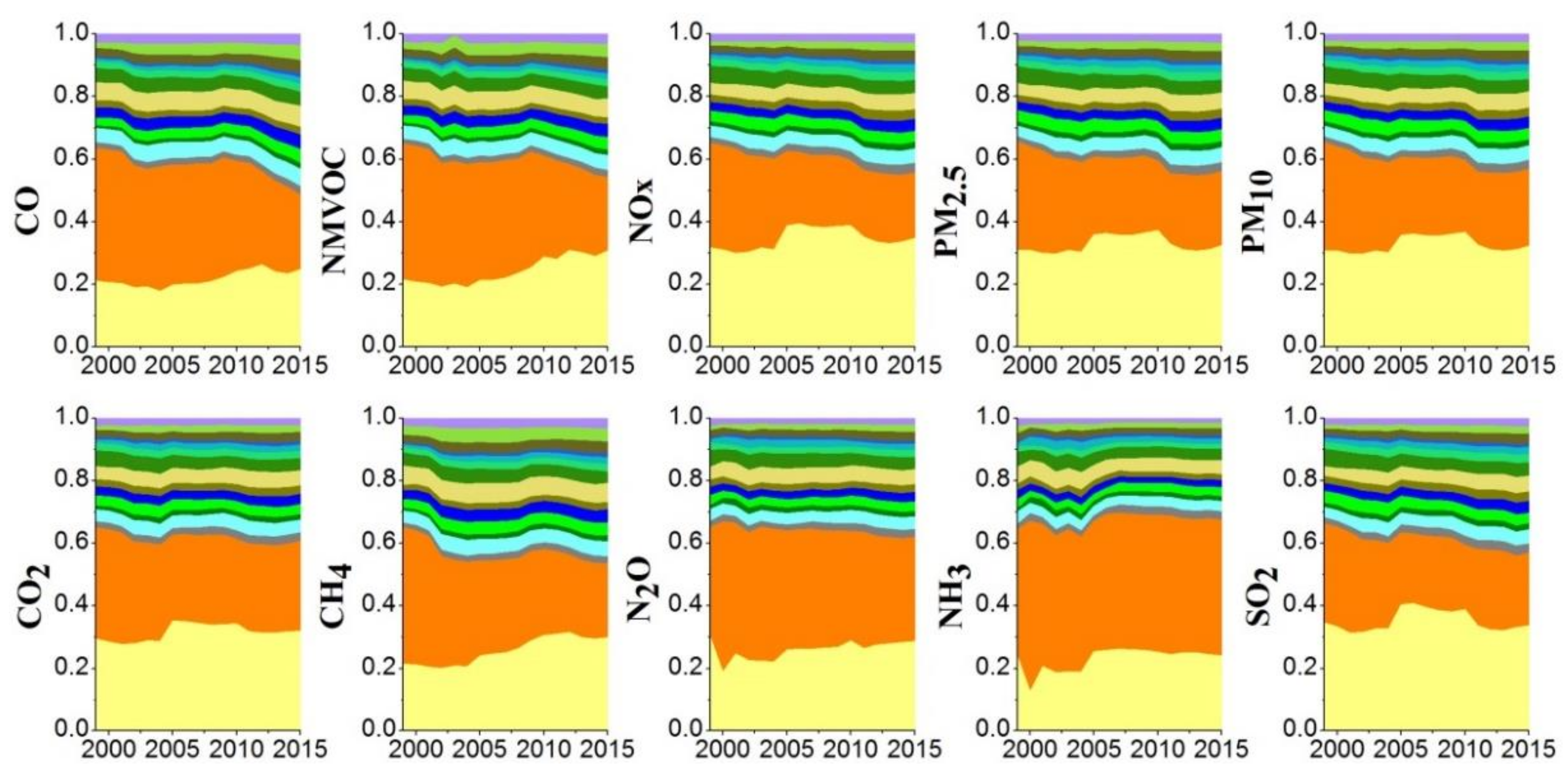
3.2. Vehicular Emissions at the City Level

The cities that made the strongest contribution rates to total vehicular pollutant emissions in the CCUA between 1999 and 2015 were Chongqing and Chengdu due to their higher economic development level and more vehicle population. The contribution rates of these two cities of vehicular CO, NMVOC, NO_x, PM_2.5, PM₁₀, CO₂, CH₄, N₂O, NH₃, and SO₂ emissions to the total region remained above 48.68%, 54.19%, 55%, 54.82%, 55.42%, 59.3%, 53.4%, 61.53%, 62.06%, and 56.06%, respectively, during the research years (Figure 6). The contribution rates of vehicular CO, NMVOC, and CH₄ emissions in Chongqing increased from 1999 to 2015 due to the increase in the population of PCs and MCs. In addition, with the rapid increase in the number of HDTs (increased from 68,025 in 2004 to 96,200 in 2005) in Chongqing, the contribution rates of vehicular NO_x, PM_2.5, PM₁₀, CO₂, and SO₂ emissions increased from 2004 to 2005. The contribution rates of vehicular CO, NMVOC, NO_X, PM_2.5, PM₁₀, CO₂, CH₄, and SO₂ emissions in Chengdu decreased from 1999 to 2015. The contribution rates of vehicular N₂O and NH₃ emissions in Chongqing and Chengdu were stable, and remained above 18.9% and 33.1%, 12.80% and 40.72%, respectively during the study period. The contributions of vehicular emissions in other cities were relatively small, but the reduction of vehicular pollutants in these cities could not relax.

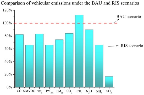
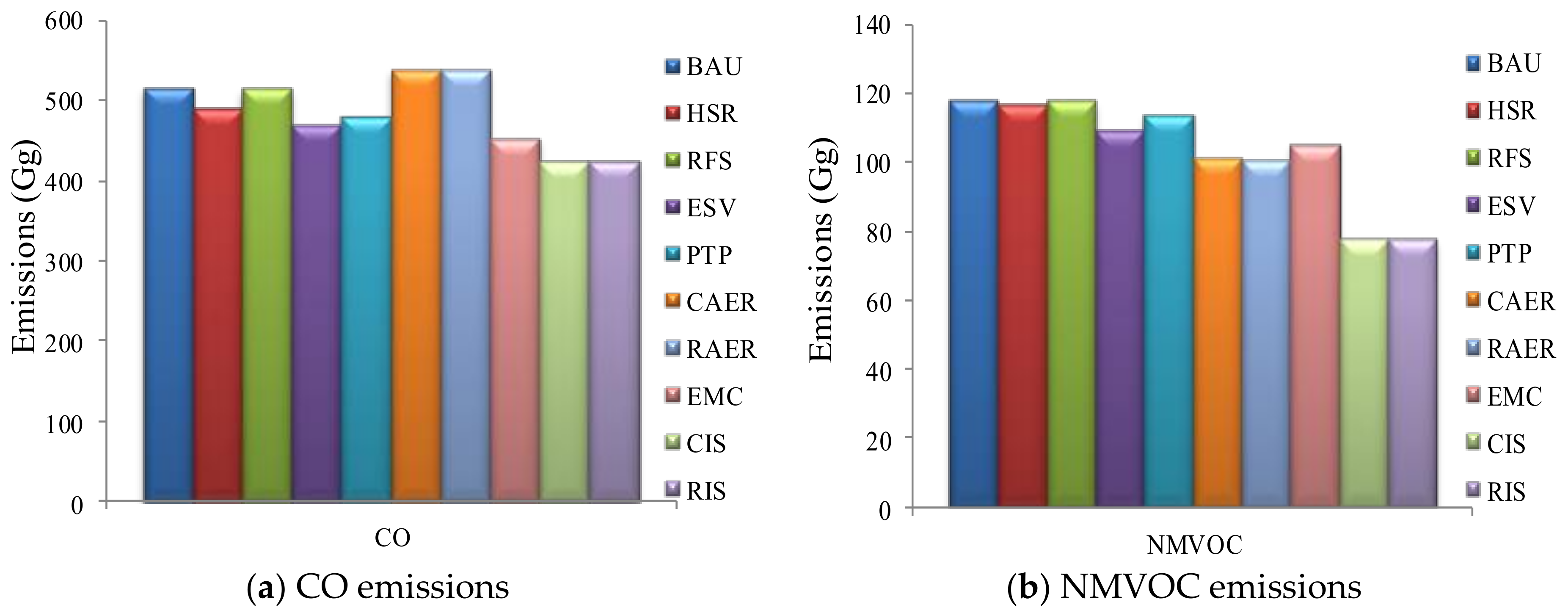
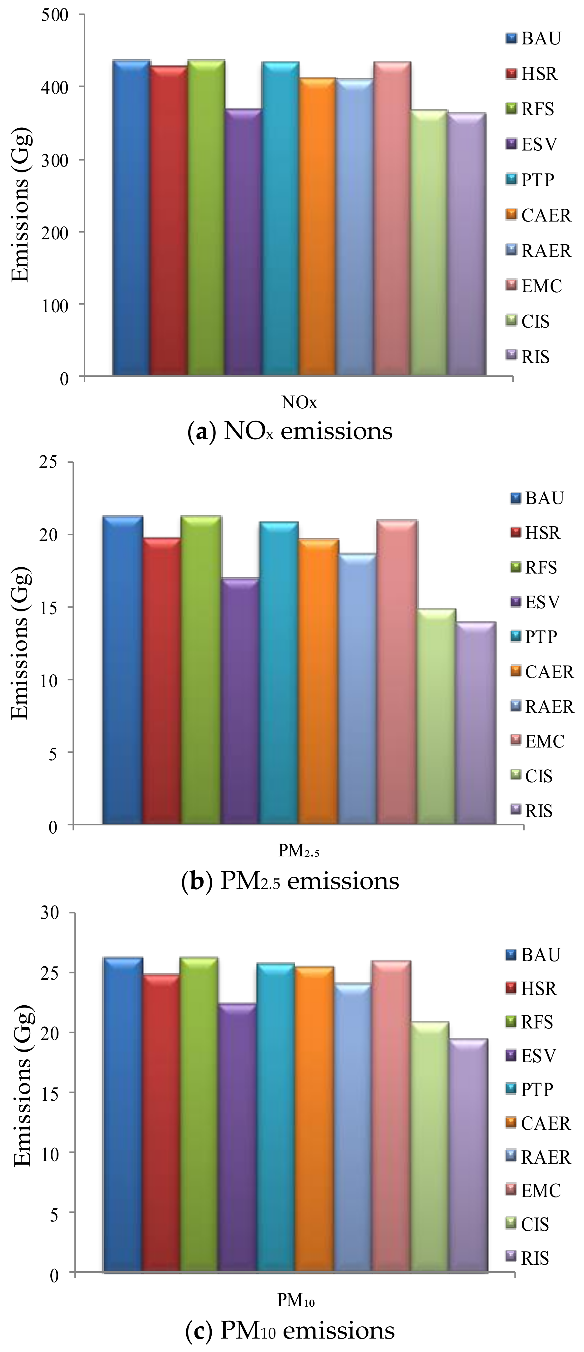
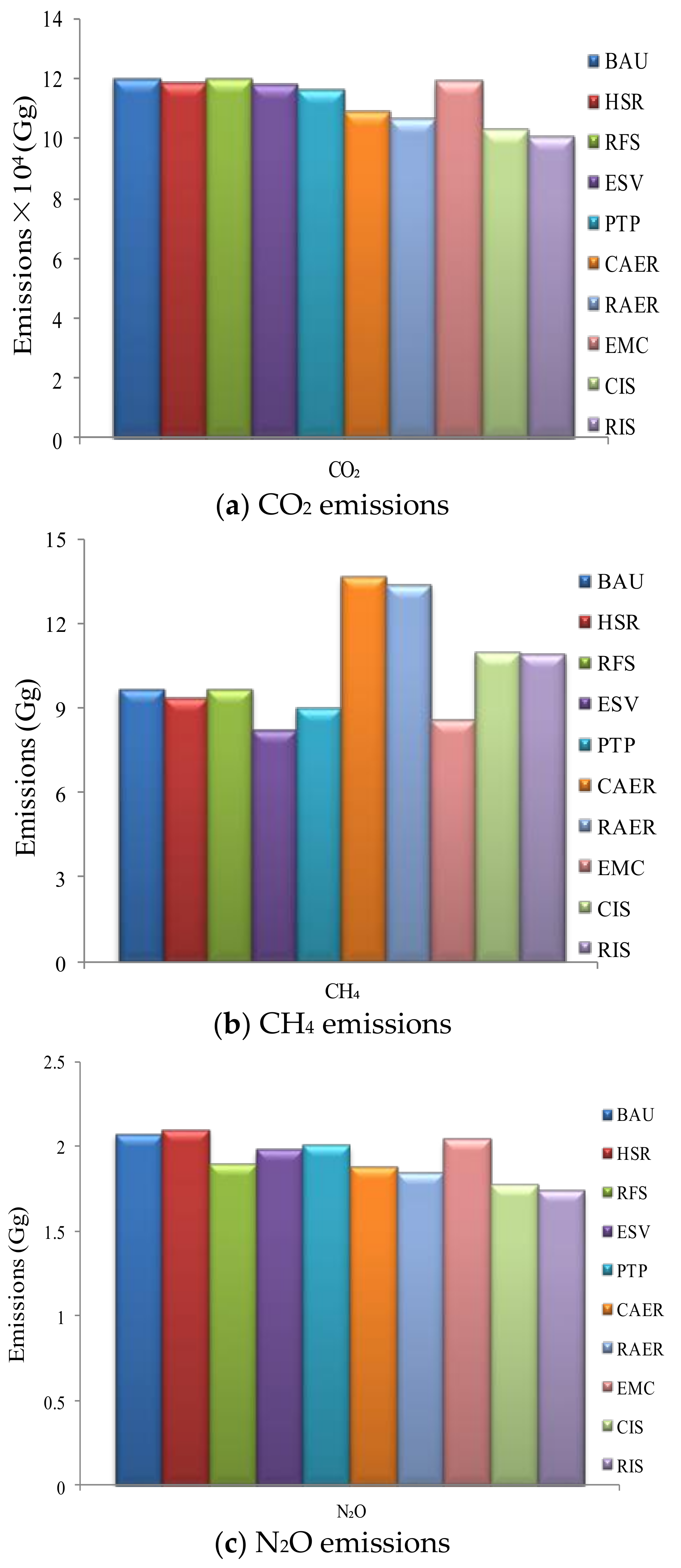
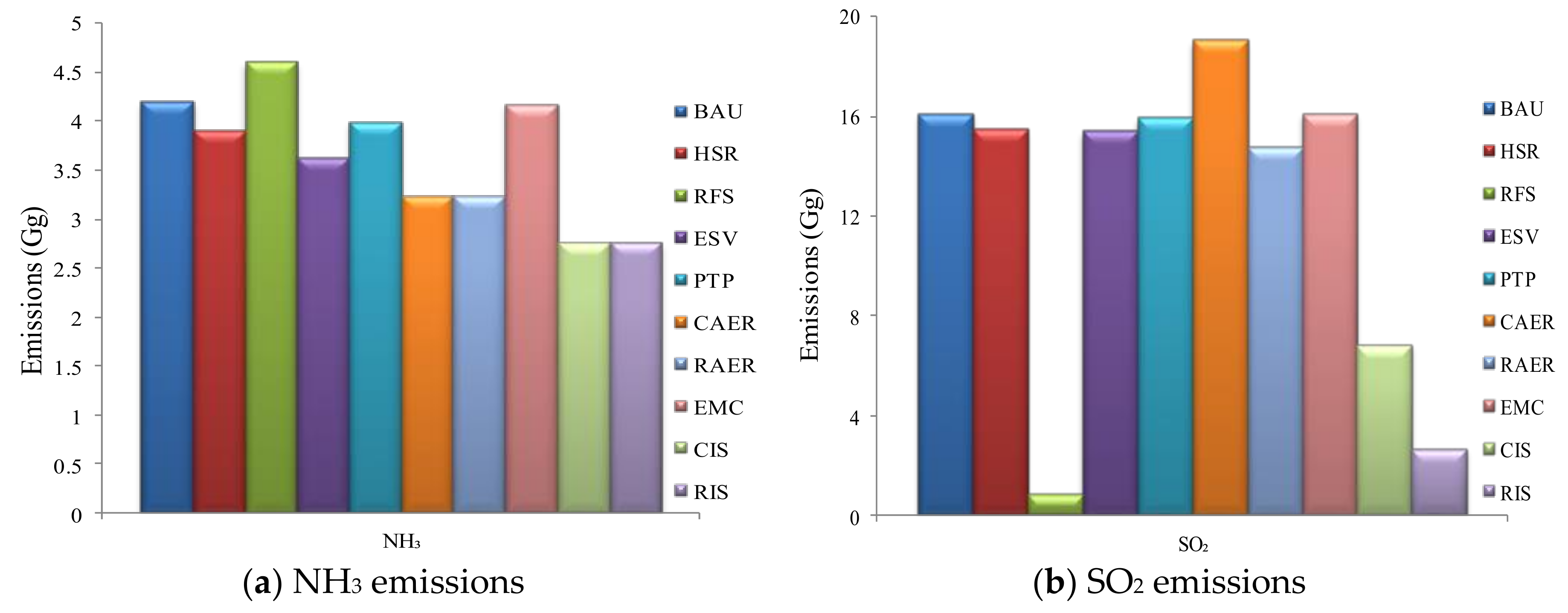
3.3. Reduction Effects of Different Control Scenarios

Inventories for vehicular CO, NMVOC, NO_x, PM_2.5, PM₁₀, CO₂, CH₄, N₂O, NH₃, and SO₂ emissions in the CCUA in 2020, under the different emission reduction scenarios described above, were calculated and compared with the vehicular emissions under the BAU scenario. The predicted vehicle population data, emission factors, and annual VKT for the different vehicle types will produce CO, NMVOC, NO_x, PM_2.5, PM₁₀, CO₂, CH₄, N₂O, NH₃, and SO₂ emissions of 515.5, 118.1, 438.3, 21.3, 26.3, 120359.3, 9.7, 2.07, 4.2, and 16.14 Gg, respectively, in the CCUA under the BAU scenario in 2020.

Emissions of CO will be lower in 2020 under each of the different scenarios than under the BAU scenario except for the CAER and RAER scenarios (Figure 7). The CAER and RAER scenarios will increase CO emissions by 4.39% and 4.29%, relative to the BAU scenario. The emission reduction effect of electric vehicles on vehicular pollutant CO will be offset by the development of natural gas vehicles when electric vehicles and natural gas vehicles are promoted at the same time, so the CO emission reduction effect will not be obvious. Emissions of NMVOC will be lower in 2020 under each of the nine test scenarios than under the BAU scenario (Figure 7). The CAER and RAER scenarios result in more of a decrease in NMVOC emissions reduction effect than the other single scenarios, and decrease by 14.21% and 14.43%, respectively, relative to the BAU scenario. The CAER scenario and RAER scenario differed little in terms of decreasing emissions, indicating that NMVOC are predominantly emitted when vehicles are driven, meaning emissions are barely affected by an upstream in changes to power sources. The CIS scenario and RIS scenario yielded notable decreases in emissions. The CIS scenario decreased CO and NMVOC emissions by 17.76% and 34.02%, respectively, and the RIS scenario decreased CO and NMVOC emissions by 17.86% and 34.24%, respectively.

All nine scenarios will decrease NO_x, PM_2.5, and PM₁₀ emissions in the CCUA in 2020, relative to the BAU scenario (Figure 8). The ESV scenario will decrease NO_x, PM_2.5, and PM₁₀ emissions by 15.53%, 20.33%, and 15.03%, respectively, relative to the BAU scenario, and the other single scenarios decreased NO_x, PM_2.5, and PM₁₀ emissions to lesser degrees. Vehicles using new energy sources (electric, hybrid, and natural gas-powered vehicles) emit less NO_x than traditional vehicles, and the CAER scenario and RAER scenario will decrease NO_x emissions by 5.65% and 6.33%, respectively, relative to the BAU scenario. Guo et al. (2016) [13] researched the reduction potential of vehicular emissions in Beijing and concluded that ESV scenario could reduce the emissions of the NO_x and PM₁₀ significantly, and the effect of the AER scenario seemed slight. In addition, the CIS scenario will decrease NO_x, PM_2.5, and PM₁₀ emissions by 16.16%, 30.01%, and 20.62%, respectively, and the RIS scenario will decrease NO_x, PM_2.5, and PM₁₀ emissions by 16.82%, 34.14%, and 25.86%, respectively.

The nine emission reduction scenarios will decrease CO₂ emissions, relative to the BAU scenario (Figure 9). The CAER scenario and RAER scenario will decrease CO₂ emissions by 9.12% and 11.12%, respectively, relative to the BAU scenario. In addition, the CIS scenario and RIS scenario will decrease CO₂ emissions of 14.15% and 16.08%, respectively, relative to the BAU scenario. The ESV scenario will decrease CH₄ emissions by 15.07%, relative to the BAU scenario, and the other scenarios will decrease CH₄ emissions to lesser degrees. The CAER scenario and RAER scenario will increase CH₄ emissions by 41.23% and 38.29%, respectively, and this is because the CCUA has a large proportion of natural gas vehicles. The CIS scenario and RIS scenario will give increases in emissions of 13.59% and 12.62%, respectively. The RFS scenario will decrease N₂O emissions by 8.65%, relative to the BAU scenario. The RAER scenario will give a decrease in N₂O emissions of 10.85%, relative to the BAU scenario. However, the N₂O emission factors for HDT and BUS increased between the State I and State V regulations [36], resulting in the HSR scenario increasing N₂O emissions by 1.19%, relative to the BAU scenario.

The different scenarios will give different decrease trends in NH₃ emissions relative to the BAU scenario (Figure 10). However, the RFS scenario will increase NH₃ emissions by 9.76% relative to the BAU scenario. This is because vehicles usually use three-way catalytic converters to reduce NO_x to nitrogen to decrease NO_x emissions. Three-way catalytic converters do not produce large amounts of NH₃ when the oil quality is relatively poor, but NH₃ emissions increase as the oil quality improves [56]. The main component of fog and haze in China is PM_2.5 [57], and NH₃ emitted by vehicles is essential to the formation and growth of PM_2.5. There is a clear need to decrease NH₃ emissions. The RFS scenario will decrease SO₂ emissions by 94.81%, relative to the BAU scenario. This is a larger decrease than for the other scenarios because vehicular SO₂ emissions were mainly controlled by vehicle population and the sulfur content in fuel [59]. The CAER scenario will increase SO₂ emissions by 18.19%, relative to the BAU scenario because the upstream power for electric vehicles is mainly produced by coal-fired power plants. Promoting natural gas-powered vehicles could decrease SO₂ emissions, but this would be offset by upstream SO₂ emissions to produce power for electric vehicles. Therefore, the RAER scenario (using “clean” energy to power electric vehicles) is much better than the CAER scenario.

In summary, IS scenario could reduce vehicular emissions in the short term, except for CH₄, although the population of vehicles would increase in the next five years. This is consistent with the conclusion of scenario analysis to vehicular emission reduction in Beijing-Tianjin-Hebei region [13]. So, emissions will be decreased only to a relatively limited extent by a single pollution control policy, but implementation of all policies together will decrease emissions more effectively. Therefore, the control of vehicular pollution in the CCUA will require comprehensive policy formulation. Promotion of natural gas vehicles has an advantage of reducing energy consumption and vehicular NO_x, PM_2.5, and PM₁₀ emissions, but has a disadvantage of reducing CO and greenhouse gases emissions. Therefore, the promotion of natural gas vehicles in the future will need to comprehensively consider the advantages and disadvantages of pollutant emissions.

4. Conclusions

In this work, the vehicular emission inventories of ten pollutants (including CO, NMVOC, NO_x, PM_2.5, PM₁₀, CO₂, CH₄, N₂O, NH₃, and SO₂) in the CCUA from 1999 to 2015 were estimated. Vehicular emissions of CO, NMVOC, CH₄, and SO₂ showed a downtrend, and NO_x, PM_2.5, PM₁₀, and N₂O showed an uptrend in recent years. Vehicular emissions of CO₂ and NH₃ increased markedly between 1999 and 2015. Chengdu and Chongqing were the dominant contributors of vehicular emissions in the CCUA.

Vehicular NMVOC, NO_x, and CO₂ emissions were lower for each emission reduction scenario than for BAU scenario. CO and CH₄ emissions were higher under the CAER and RAER scenarios as they have a large proportion of natural gas vehicles. Emissions of PM_2.5, PM₁₀, and SO₂ were obviously lower under the RAER scenario than the CAER scenario as coal-fired power plants are the main sources of electricity in China. The RIS scenario could achieve the maximum emission reduction of vehicular pollutants CO, NMVOC, NO_x, PM_2.5, PM₁₀, CO₂, N₂O, and NH₃ and reduction rates were 17.86%, 34.24%, 16.82%, 34.14%, 25.86%, 16.08%, 16.08%, and 34.24%, respectively. Whereas, the ESV scenario and RFS scenario could reduce the vehicular CH₄ and SO₂ emissions more effectively as reduction rates were 15.07% and 94.81%, respectively.

Although these static emissions inventories cannot completely identify the actual vehicular emissions in this area due to the complexity of the vehicle activities, the emission reduction characteristics of pollutants under each reduction scenario can still provide references for policy-making. In addition, a scientifically and rational air pollution control strategy would minimize emissions and take into account the effect evaluation and cost-effectiveness of the control strategy. It will be necessary to assess the cost-effectiveness of the control scenarios. The optimal control strategy should be selected from the cost-effectiveness ratios for the control scenarios obtained by estimating the costs and health benefits of improving air quality. This would be a scientific decision-making basis for regional vehicle pollution controls and would assist decision-makers in selecting the optimal control strategy.

References

1. Lang, J.; Cheng, S.; Wei, W.; Zhou, Y.; Wei, X.; Chen, D. A study on the trends of vehicular emissions in the Beijing—Tianjin—Hebei (BTH) region, China. Atmos. Environ. 2012, 62, 605–614. [Google Scholar] [CrossRef]
2. Fu, X.; Wang, S.; Zhao, B.; Xing, J.; Cheng, Z.; Liu, H.; Hao, J. Emission inventory of primary pollutants and chemical speciation in 2010 for the Yangtze River Delta region, China. Atmos. Environ. 2013, 70, 39–50. [Google Scholar] [CrossRef]
3. Caraiani, C.; Lungu, C.I.; Dascalu, C. Energy consumption and GDP causality: A three-step analysis for emerging European countries. Renew. Sustain. Energy Rev. 2015, 44, 198–210. [Google Scholar] [CrossRef]
4. National Bureau of Statistics of China (NBSC). Chinese Statistical Yearbook; China Statistics Press: Beijing, China, 2000–2016. Available online: http://www.stats.gov.cn/tjsj/ndsj/ (accessed on 15 November 2019).
5. Ministry of Ecology and Environment of the People’s Republic of China (MEEPRC). China Vehicle Environmental Management Annual Report; Ministry of Ecology and Environment of the People’s Republic of China (MEEPRC): Beijing, China, 2016. [Google Scholar]
6. Wang, H.; Chen, C.; Huang, C.; Fu, L. On-road vehicle emission inventory and its uncertainty analysis for Shanghai, China. Sci. Total Environ. 2008, 398, 60–67. [Google Scholar] [CrossRef]
7. Lang, J.; Tian, J.; Zhou, Y.; Li, K.; Chen, D.; Huang, Q.; Xing, X.; Zhang, Y.; Cheng, S. A high temporal-spatial resolution air pollutant emission inventory for agricultural machinery in China. J. Clean. Prod. 2018, 183, 1110–1121. [Google Scholar] [CrossRef]
8. Ghose, M.K.; Paul, R.; Banerjee, S.K. Assessment of the impact of vehicle emissions on urban air quality and its management in Indian context: The case of Kolkata (Calcutta). Environ. Sci. Policy 2004, 7, 345–351. [Google Scholar] [CrossRef]
9. Kota, S.H.; Zhang, H.; Chen, G.; Schade, G.W.; Ying, Q. Evaluation of on-road vehicle CO and NOx National Emission Inventories using an urban-scale source-oriented air quality model. Atmos. Environ. 2014, 85, 99–108. [Google Scholar] [CrossRef]
10. Fameli, K.; Assimakopoulos, V. Development of a road transport emission inventory for Greece and the Greater Athens Area: Effects of important parameters. Sci. Total Environ. 2015, 505, 770–786. [Google Scholar] [CrossRef]
11. Tian, J. Atmospheric Environment Impact Assessment of Mobile Source and Vehicle Control Strategies in Nanjing. Master’s Thesis, Nanjing University, Jiangsu, China, 2013. (In Chinese). [Google Scholar]
12. Li, Y.Y. Research on Total Amount of Vehicular Emissions in Beijing-Tianjin-Hebei (BTH) Region and its Abatement Control Strategy. Master’s Thesis, Tianjin University of Technology, Tianjin, China, 2015. (In Chinese). [Google Scholar]
13. Guo, X.; Fu, L.; Ji, M.; Lang, J.; Chen, D.; Cheng, S. Scenario analysis to vehicular emission reduction in Beijing-Tianjin-Hebei (BTH) region. Chin. Environ. Pollut. 2016, 216, 470–479. [Google Scholar] [CrossRef]
14. National Bureau of Statistics of Sichuan (NBSS). Sichuan Statistical Yearbook; China Statistics Press: Beijing, China, 2000–2016. Available online: http://tjj.sc.gov.cn/tjcbw/tjnj/ (accessed on 15 November 2019).
15. National Bureau of Statistics of Chongqing (NBSCQ). Chongqing Statistical Yearbook; China Statistics Press: Beijing, China, 2000–2016. Available online: http://tjj.cq.gov.cn/tjsj/shuju/tjnj/ (accessed on 15 November 2019).
16. China Automotive Technology & Research Center (CATRC). China Automotive Industry Yearbook; China Automotive Industry Yearbook Press: Tianjin, China, 2000–2016. [Google Scholar]
17. Wang, H.; Fu, L.; Zhou, Y.; Du, X.; Ge, W. Trends in vehicular emissions in China’s mega cities from 1995 to 2005. Environ. Pollut. 2010, 158, 394–400. [Google Scholar] [CrossRef]
18. Sun, S.; Jiang, W.; Gao, W. Vehicle emission trends and spatial distribution in Shandong province, China, from 2000 to 2014. Atmos. Environ. 2016, 147, 190–199. [Google Scholar] [CrossRef]
19. Hao, Y.P.; Song, X.W. Research on trends and spatial distribution of vehicular emissions and its control measure assessment in the Yangtze River Delta, China, for 1999-2015. Environ. Sci. Pollut. Res. 2018, 25, 36503–36517. [Google Scholar] [CrossRef] [PubMed]
20. Dargay, J.; Gately, D. Vehicle ownership to 2015: Implications for energy use and emissions. Energy Policy 1997, 25, 1121–1127. [Google Scholar] [CrossRef]
21. Dargay, J.; Gately, Y.D. Income’s effect on car and vehicle ownership, worldwide: 1960–2015. Transp. Res. Part A Policy Pract. 1999, 33, 101–138. [Google Scholar] [CrossRef]
22. Ji, M.; Guo, X.; Lang, J. Scenario prediction of motor vehicle emission and control in megacities. Res. Environ. Sci. 2013, 26, 919–928. (In Chinese) [Google Scholar]
23. Ma, N. The Study of Pollution State of Vehicle and Partake Rate of Chongqing. Master’s Thesis, Chongqing University, Chongqing, China, 2008. (In Chinese). [Google Scholar]
24. Guo, P.; Ma, N.; Chen, G.; Qiao, Q.; Qin, Y.; Wei, X. A study on the vehicle emission factors in Chongqing. J. Southwest Univ. Nat. Sci. 2009, 31, 108–113. (In Chinese) [Google Scholar]
25. Lin, X.; Tang, D.; Ding, Y.; Yin, H.; Ji, Z. Study on the distribution of vehicle mileage traveled in China. Res. Environ. Sci. 2009, 22, 377–380. (In Chinese) [Google Scholar]
26. Huo, H.; Zhang, Q.; He, K.; Yao, Z.; Wang, X.; Zheng, B.; Streets, D.G.; Wang, Q.; Ding, Y. Modeling vehicle emissions in different types of Chinese cities: Importance of vehicle fleet and local features. Environ. Pollut. 2011, 159, 2954–2960. [Google Scholar] [CrossRef]
27. Yao, Z.; Wang, Q.; Wang, X.; Zhang, Y.; Shen, X.; Yin, H.; He, K. Emission inventory of unconventional pollutants from vehicles in typical cities. Environ. Pollut. Control 2011, 33, 96–101. (In Chinese) [Google Scholar]
28. Yao, Z.L.; Zhang, M.H.; Wang, X.T.; Zhang, Y.Z.; Huo, H.; He, K.B. Trends in vehicular emissions in typical cities in China. China Environ. Sci. 2012, 32, 1565–1573. (In Chinese) [Google Scholar]
29. Wang, T.L. The Research of the Vehicular Emission Inventory in the Urban of Chongqing Based on IVE model. Master’s Thesis, Chongqing Jiaotong University, Chongqing, China. (In Chinese).
30. Zhang, L.; Chen, J.H.; Qian, J.; Ye, H. Establishment of emission inventory and spatial distribution research of NOx from motor vehicles on Chengdu city. Sichuan Environ. 2016, 35, 95–98. (In Chinese) [Google Scholar]
31. Wang, Q.D.; He, K.B.; Yao, Z.L.; Huo, H. Research in motor vehicle driving cycle of Chinese cities. Environ. Pollut. Control 2007, 29, 745–748. (In Chinese) [Google Scholar]
32. Huo, H.; Zhang, Q.; He, K.; Yao, Z.; Wang, M. Vehicle-use intensity in China: Current status and future trend. Energy Policy 2012, 43, 6–16. [Google Scholar] [CrossRef]
33. Cai, H.; Xie, S. Estimation of vehicular emission inventories in China from 1980 to 2005. Atmos. Environ. 2007, 41, 8963–8979. [Google Scholar] [CrossRef]
34. Wang, H.; Fu, L.; Lin, X.; Zhou, Y.; Chen, J. A bottom-up methodology to estimate vehicle emissions for the Beijing urban area. Sci. Total. Environ. 2009, 407, 1947–1953. [Google Scholar] [CrossRef] [PubMed]
35. China Meterological Administration (CMA). China Meteorological Yearbook; China Meteorological Press: Beijing, China, 2000–2016. [Google Scholar]
36. Cai, H.; Xie, S.D. Determination of emission factors from motor vehicles under different emission standards in China. Acta Sci. Nat. Univ. Peking 2010, 46, 319–326. (In Chinese) [Google Scholar]
37. Che, W.W. A Highly Resolved Mobile Source Emission Inventory in the Pearl River Delta and Assessment of Motor Vehicle Pollution Control Strategies. Master’s Thesis, South China University of Technology, Guangdong, China, 2010. (In Chinese). [Google Scholar]
38. Zhang, S.J. Characteristics and Control Strategies of Vehicle Emissions in Typical Cities of China. Ph.D. Thesis, Tsinghua University, Beijing, China, 2014. (In Chinese). [Google Scholar]
39. Tao, S.C. Emission Inventory and Control Strategies of Road Mobile Sources in Guanzhong Metropolitan Area. Master’s Thesis, Chang’an University, Xi’an, China, 2016. (In Chinese). [Google Scholar]
40. Lumbreras, J.; Valdés, M.; Borge, R.; Rodríguez, M. Assessment of vehicle emissions projections in Madrid (Spain) from 2004 to 2012 considering several control strategies. Transp. Res. Part A Policy Pract. 2008, 42, 646–658. [Google Scholar] [CrossRef]
41. Liu, H.; Wang, H.W.; Luo, Q.; Wang, Y.; Ouyang, M. Energy, environmental and economic assessment of life cycle for electric vehicle. Technol. Econ. Areas Commun. 2007, 9, 45–48. (In Chinese) [Google Scholar]
42. Song, G.H.; Yu, L.; Mo, F.; Zhang, X. A comparative experimental study on the emissions of HEV and conventional gasoline vehicle. Automot. Eng. 2007, 29, 865–869. (In Chinese) [Google Scholar]
43. Zhou, Y.; Wu, Y.; Lin, B.H.; Wang, R.J.; Fu, L.X.; Hao, J.M. Assessment of the environmental effects if the compressed natural gas bus fleet in Beijing. Acta Sci. Circumstantiae 2010, 30, 1921–1925. (In Chinese) [Google Scholar]
44. Li, S.H. Life Cycle Assessment and Environmental Benefits Analysis of Electric Vehicles. Ph.D. Thesis, Jilin University, Changchun, China, 2014. (In Chinese). [Google Scholar]
45. Yu, M.X. The Emission Ceiling Control of NOx for Light-Duty Vehicles in Three Developed Regions of China. Master’s Thesis, Tsinghua University, Beijing, China, 2014. (In Chinese). [Google Scholar]
46. Wang, R.J. Fuel-Cycle Assessment of Energy and Environmental Impacts from Electric Vehicles and Natural Gas Vehicles. Ph.D. Thesis, Tsinghua University, Beijing, China, 2015. (In Chinese). [Google Scholar]
47. International Energy Agency (IEA). World Energy Outlook 2013; International Energy Agency: Paris, France, 2013. [Google Scholar]
48. Jiang, K.J.; Hu, X.L.; Zhuang, X.; Liu, Q. China’s low-carbon scenarios and roadmap for 2050. Sino Glob. Energy 2009, 14, 1–7. (In Chinese) [Google Scholar]
49. Ma, M. Development of DeNOx technology in coal-fired power plants. Electr. Power Constr. 2004, 25, 52–55. (In Chinese) [Google Scholar]
50. Feng, D.X. Application of denitrification technologies on coal burning boiler in a coal-fired power plant. Electr. Power Environ. Prot. 2015, 21, 23–26. (In Chinese) [Google Scholar]
51. Zhao, Y.; Wang, S.; Duan, L.; Lei, Y.; Cao, P.; Hao, J. Primary air pollutant emissions of coal-fired power plants in China: Current status and future prediction. Atmos. Environ. 2008, 42, 8442–8452. [Google Scholar] [CrossRef]
52. Chen, W.Y.; Xu, R.N. Clean coal technology development in China. Energy Policy 2010, 38, 2123–2130. [Google Scholar] [CrossRef]
53. Wei, W.; Wang, S.; Chatani, S.; Klimont, Z.; Cofala, J.; Hao, J. Emission and speciation of non-methane volatile organic compounds from anthropogenic sources in China. Atmos. Environ. 2008, 42, 4976–4988. [Google Scholar] [CrossRef]
54. Zhao, B.; Wang, S.; Dong, X.; Wang, J.; Duan, L.; Fu, X.; Hao, J.; Fu, J. Environmental effects of the recent emission changes in China: Implications for particulate matter pollution and soil acidification. Environ. Res. Lett. 2013, 8, 024031. [Google Scholar] [CrossRef]
55. Zhao, B.; Wang, S.X.; Liu, H.; Xu, J.Y.; Fu, K.; Klimont, Z.; Hao, J.M.; He, K.B.; Cofala, J.; Amann, M. NOx emissions in China: Historical trends and future perspectives. Atmos. Chem. Phys. Discuss. 2013, 13, 9869–9897. [Google Scholar] [CrossRef]
56. Wang, S.X.; Zhao, B.; Cai, S.Y.; Klimont, Z.; Nielsen, C.P.; Morikawa, T.; Woo, J.H.; Kim, Y.; Fu, X.; Xu, J.Y.; et al. Emission trends and mitigation options for air pollutants in East Asia. Atmos. Chem. Phys. Discuss. 2014, 14, 6571–6603. [Google Scholar] [CrossRef]
57. Chan, C.K.; Yao, X.H. Air pollution in mega cities in China. Atmos. Environ. 2008, 42, 1–42. [Google Scholar] [CrossRef]
58. Behera, S.N.; Sharma, M. Investigating the potential role of ammonia in ion chemistry of fine particulate matter formation for an urban environment. Sci. Total. Environ. 2010, 408, 3569–3575. [Google Scholar] [CrossRef] [PubMed]
59. Lang, J.; Zhou, Y.; Cheng, S.; Zhang, Y.; Dong, M.; Li, S.; Wang, G.; Zhang, Y. Unregulated pollutant emissions from on-road vehicles in China, 1999–2014. Sci. Total Environ. 2016, 573, 974–984. [Google Scholar] [CrossRef] [PubMed]
Figure 1. The vehicular population from 1999 to 2015 in China. This graph was prepared based on the data in the statistical yearbooks (NBSC, 2000–2016).
Sustainability 11 06503 g001
Figure 2. Location of the Chengdu-Chongqing Urban Agglomeration (CCUA) with the administrative divisions shown.
Sustainability 11 06503 g002
Figure 3. Method system construction of this study.
Sustainability 11 06503 g003
Figure 4. Predicted values of the vehicle populations in the CCUA from 2016 to 2020.
Sustainability 11 06503 g004
Figure 5. Vehicular emission trends in the CCUA between 1999 and 2015.
Sustainability 11 06503 g005
Figure 6. Contributions of different cities to total vehicular emissions in the CCUA. From top to bottom: Chongqing, Chengdu, Dazhou, Deyang, Guangan, Leshan, Luzhou, Meishan, Mianyang, Nanchong, Neijiang, Suining, Yaan, Yibin, Ziyang, Zigong.
Sustainability 11 06503 g006
Figure 7. CO and NMVOC emissions in 2020 under different emission reduction scenarios.
Sustainability 11 06503 g007
Figure 8. NOx, PM2.5, and PM10 emissions under different emission reduction scenarios.
Sustainability 11 06503 g008
Figure 9. CO2, CH4, and N2O emissions under different emission reduction scenarios.
Sustainability 11 06503 g009
Figure 10. NH3 and SO2 emissions under different emission reduction scenarios.
Sustainability 11 06503 g010