New Artificial Neural Networks Model for Predicting Rate of Penetration in Deep Shale Formation

Abstract

Rate of penetration (ROP) means how fast the drilling bit is drilling through the formations. It is known that in the petroleum industry, most of the well cost is taken by the drilling operations. Therefore, it is very crucial to drill carefully and improve drilling processes. Nevertheless, it is challenging to predict the influence of every single parameter because most of the drilling parameters depend on each other and altering an individual parameter will have an impact on the rest. Due to the complexity of the drilling operations, up to the present time, there is no reliable model that can adequately estimate the ROP. Artificial intelligence (AI) might be capable of building a predictive model from a number of input parameters that correlate to the output parameter. A real field dataset, of shale formation, that contains records of both drilling parameters such as, rotation per minute (RPM), weight on bit (WOB), drilling torque (τ), standpipe pressure (SPP) and flow pump (Q) and mud properties such as, mud weight (MW), funnel and plastic viscosities (FV) (PV), solid (%) and yield point (YP) were used to predict ROP using artificial neural network (ANN). A comparison between the developed ANN-ROP model and the number of selected published ROP models were performed. A novel empirical equation of ROP using the above-mentioned parameters was derived based on ANN technique which is able to estimate ROP with excellent precision (correlation coefficient (R) of 0.996 and average absolute percentage error (AAPE) of 5.776%). The novel ANN-based correlation outperformed three published empirical models and it can be used to predict the ROP without the need for artificial intelligence software.

1. Introduction

Drilling operations are the backbone of the oil and gas industry. They can be very expensive and therefore, they require several economical and safety concerns. Improving oilfield operations requires active monitoring drilling performance to insure minimize drilling costs. Much effort has been excelled to avoid drilling difficulties and enhance the drilling process. Typically, drilling cost is directly related to drilling speed. Therefore, achieving an adequate rate of penetration (ROP) ensures optimal drilling process and accordingly a reduced drilling cost. Thus, various parameters that affect ROP should be optimally controlled.

Rate of penetration (ROP) means how fast the drilling bit is drilling through the formations. It captures the speed or the movement of the drilling bit when it breaks the rocks, and it is identified in field units as ft/h [1]. Notoriously, in the oil and gas industry, most of the well cost is taken by the drilling operations. Therefore, it is very crucial to drill carefully and improve drilling processes. Nevertheless, it is challenging to predict the influence of every single parameter because most of the drilling parameters depend on each other and altering an individual parameter will have an impact on the rest. Moreover, ROP assists the drilling engineer to define the best drilling parameters to accomplish the lowest cost per foot [2]. Whereas, many challenges can occur during drilling operations under high ROP such as stuck pipe and poor hole cleaning. Therefore, it is important to select the optimal drilling parameters for ROP that cause no drilling problems [3].

Many parameters affect ROP such as formation properties, drilling fluid properties, hydraulic and mechanical parameters, and rig efficiency [4]. Hossain and Al-Majed [5] categorized these parameters into two groups: environmental and controllable parameters. Environmental factors are those, which are created by nature or drilling conditions that are difficult to change, for example, mud properties are usually difficult to change because of some drilling objectives, which attained only by requiring a specific volume of the mud such as overbalance drilling to prevent the flow of formation fluid. On the contrast, controllable factors are those, which can be altered such as rotary speed, weight on bit and hydraulic parameters.

Many methods propose relationships between different parameters and ROP. Maurer [6] proposed a theoretical model for roller cone bits based on rotary speed, weight on bit, rock strength, and bit size. He developed his equation based on observation such as the volume of cuttings that created as shown in Equation (1).

$$\mathrm{ROP}=\mathrm{k}\frac{{\mathrm{N} \mathrm{W}}^2}{{\mathrm{d}}_{\mathrm{b}}{}^2{ \mathrm{S}}^2}$$

(1)

where k is drillability constant, N is rotary speed (RPM), W is weight on bit (Klb_f), d_b is the diameter of the bit (in), and S is rock compressive strength (kPa)

Bingham [7] modified the Maurer model into a simple equation that also neglects the drilling depth as shown in Equation (2). He introduced weight exponent ($a5$) based on laboratory experiments.

$$\mathrm{ROP}=\mathrm{K}{\left(\frac{\mathrm{W}}{{\mathrm{d}}_{\mathrm{b}}}\right)}^{a_5}\mathrm{N}$$

(2)

Bourgoyne and Young’s [8] introduced one of the most significant models of predicted ROP using multiple regression analysis of drilling parameters using Equation (3).

$$\begin{array}{c}\mathrm{ROP}={\mathrm{f}}_1\times {\mathrm{f}}_2\times {\mathrm{f}}_3\times {\mathrm{f}}_4\times {\mathrm{f}}_5\times {\mathrm{f}}_6\times {\mathrm{f}}_7\times {\mathrm{f}}_8\\ \begin{array}{cc}{\mathrm{f}}_1={\mathrm{e}}^{{\mathrm{a}}_1}& {\mathrm{f}}_2={\mathrm{e}}^{{\mathrm{a}}_2 \left(10000-\mathrm{TVD}\right)}\\ {\mathrm{f}}_3={\mathrm{e}}^{{\mathrm{a}}_3{ \mathrm{TVD}}^{0.69}\left({\mathrm{EMW}}_{\mathrm{pore}}-67.41\right)}& {\mathrm{f}}_4={\mathrm{e}}^{{\mathrm{a}}_4 \mathrm{TVD}\left({\mathrm{EMW}}_{\mathrm{pore}}-\mathrm{ECD}\right)}\\ {\mathrm{f}}_5={\left(\frac{\left(\frac{\mathrm{w}}{{\mathrm{d}}_{\mathrm{b}}}\right) -{\left(\frac{\mathrm{w}}{{\mathrm{d}}_{\mathrm{b}}}\right)}_{\mathrm{t}}}{4-{\left(\frac{\mathrm{w}}{{\mathrm{d}}_{\mathrm{b}}}\right)}_{\mathrm{t}}}\right)}^{{\mathrm{a}}_5}& {\mathrm{f}}_6={\left(\frac{\mathrm{N}}{60}\right)}^{{\mathrm{a}}_6}\\ {\mathrm{f}}_7={\mathrm{e}}^{{\mathrm{a}}_7 \mathrm{h}}& {\mathrm{f}}_8={\left(\frac{{\mathrm{F}}_{\mathrm{j}}}{1000}\right)}^{{\mathrm{a}}_8}\end{array}\end{array}$$

(3)

where TVD is the true vertical depth (ft), EMW_pore is pore equivalent mud weight (pcf), ECD is the equivalent circulation density (pcf, bound per cubic feet), F_j is impact factor (lb), N is rotation per minute (RPM), W is the bit weight (K_lbf), d_b is the diameter of the bit (in), ${\mathrm{f}}_1$ is the formation strength effects, ${\mathrm{f}}_2$ and ${\mathrm{f}}_3$ are the compaction effects, ${\mathrm{f}}_4$ is the overbalance effects, ${\mathrm{f}}_5$ and ${\mathrm{f}}_6$ are the rotary speed and bit weight effects, ${\mathrm{f}}_7$ is the tooth wear effects, and ${\mathrm{f}}_8$ is the bit hydraulic effects. The constants ${\mathrm{a}}_1$to ${\mathrm{a}}_8$ be found for each formation based on local legacy drilling data.

Warren [9] proposed a special cleaning ROP model for bit in the soft formation where the removal of cutting has no obstruction on ROP. The model is based on the relationship between rock and bit on one hand and the effects of bit wear, chips hold down, cutting removal and cutting generation on the other. Warren’s model calculates ROP using Equation (4).

$$\mathrm{ROP}={\left(\frac{{\mathrm{a} \mathrm{S}}^2{\mathrm{d}}_{\mathrm{b}}^3}{{\mathrm{N}}^{\mathrm{b}}{ \mathrm{W}}^2}+\frac{\mathrm{c}}{{\mathrm{N} \mathrm{d}}_{\mathrm{b}}}\right)}^{-1}$$

(4)

where a, b and c are constants of the bit.

Hareland [10] modified Warren model by adding a dimensional analysis containing drilling fluid properties and modified impact force and bit wear as shown in Equation (5).

$$\mathrm{ROP}=\left[1-\frac{{\mathrm{W}}_{\mathrm{c}}{{\displaystyle \sum }}_{\mathrm{i}=1}^{\mathrm{n}}{\mathrm{W}}_{\mathrm{i}}{ \mathrm{N}}_{\mathrm{i}}{ \mathrm{A}}_{\mathrm{abr},\mathrm{i}}{ \mathrm{S}}_{\mathrm{i}}}{8}\right]{\left[{\mathrm{f}}_{\mathrm{c}}\left({\mathrm{P}}_{\mathrm{e}}\right)\left(\frac{{\mathrm{a} \mathrm{S}}^2{\mathrm{d}}_{\mathrm{b}}^3}{{\mathrm{N}}^{\mathrm{b}}{ \mathrm{W}}^2}+\frac{\mathrm{c}}{{\mathrm{N} \mathrm{d}}_{\mathrm{b}}}\right)+\frac{{\mathrm{d}\mathsf{\mu }\mathsf{\gamma }\mathrm{d}}_{\mathrm{b}}}{{\mathrm{F}}_{\mathrm{jm}}}\right]}^{-1}$$

(5)

where W_c is wear coefficient, A_abr is relative abrasiveness, ${\mathrm{f}}_{\mathrm{c}}\left({\mathrm{P}}_{\mathrm{e}}\right)$ chip hold down function (lb_f), $\mathsf{\mu }$ is mud viscosity (cP), $\mathsf{\gamma }$ is fluid specific gravity, F_jm is modified impact force (lb_f), and a, b, c, d are constants.

The aim of this study is to introduce a reliable artificial neural network (ANN) predictive model for ROP using drilling data and drilling-mud properties. The outcome attained from the ANN was compared with ROP models to illustrate the model accuracy based on the highest R and the minimum average absolute percentage error (AAPE).

1.1. Artificial Intelligence (AI)

AI is made to allow computers to accomplish tasks that were difficult to be achieved, such as visual perception, decision-making, speech recognition, language translation, and image processing. The purpose of artificial intelligence is to develop a model or algorithm which needs machines to achieve tasks that obviously require knowledge, understanding, and experience when performed by humans.

1.2. Artificial Neural Networks (ANN)

Normally, ANN contains an input layer, number of hidden layers (middle layers), and an output layer. The input layer receives information, hidden layers develop a relationship between the parameters, and then the output layer forms the results [11]. Optimization is required to select the appropriate numbers of layers and neurons because choosing many neurons results in over-fitting and choosing a few neurons results in under-fitting [12]. Increasing the model size by increasing the numbers of hidden layers and neurons results in increasing the computational time and leads to memorization, which is decreasing the error during model training whereas the error remains high during testing the unseen data [13]. Too much training also causes overfitting. To reduce the overfitting issues, it is suggested to perform the criteria of early stopping while some of the data is devoted to validation reasons.

Modeling the network commences with the training process starting by feeding the data into the input layer, then to the hidden layer and finally the output layer where the actual data is compared with the predicted data [14]. The difference between the estimated and actual data is feedback to the model to modify the weights and biases. This procedure is called the epoch. In this method, all the training dataset is trained continuously until the average error decreases to certain known limit [15]. Figure 1 presents the ANN architecture used in this study. Model development will be discussed in the following sections.

1.3. Application of AI in ROP Prediction

Many mathematical models have been introduced to predict the rate of penetration from different parameters. Nevertheless, no single relationship satisfactory predicts ROP. Mostly because of the complex effect of the parameters describing the ROP and additionally due to incomplete understanding of the relationships between the ROP and some of these parameters. Therefore, many researchers tried to use AI to attain a reliable ROP predictive model.

Bilgesu [16] used the ANN tool to model ROP and the bit wear for various types of formation and operating parameters. He used 500 dataset records of nine input parameters including RPM, WOB, torque, Q, rotating time, tooth wear, bearing wear, formation abrasiveness and formation drillability. He trained his model using 90% of the data and the remaining 10% for testing. He achieved a correlation coefficient (R) that ranged from (0.902) to (0.982).

Moran [17] used ANN to study legacy-drilling data and improved the prediction of ROP. He used six input parameters including RPM, WOB, MW, rock strength, abrasion and type of the rock. He achieved a coefficient of determination of R² = 0.8 between ANN-predicted ROP and legacy-data ROP.

Jahanbakhshi [18] used ANN to predict ROP based on offset well data. He used large number of input parameters, 21, which include rotary speed, weight on bit, pump pressure, equivalent circulating density, mud type, yield point, plastic viscosity, mud pH, solid percent, 10 minute gel strength, 10 s gel strength, bit wear, bit type, bit hydraulic power, density of rock, porosity, permeability, formation drillability, differential pressure, hole depth and hole size. He arranged 70% of the data for model training, 15% for model validation and 15% for model testing. He achieved a correlation coefficient of R² = 0.916 and mean square error of MSE = 0.015 for the testing data.

Arabjamaloei [19] used ANN to build a predictive model for ROP. He used 330 data records of ten input parameters including rotary speed, weight on bit, flow rate, mud density, viscosity, depth, bit size, bit hours, bit efficiency and annulus pressure. He achieved a coefficient of determination of R² = 0.9402 in model training and R² = 0.7401 in model testing.

Bataee [20] also used ANN to predict ROP and improve drilling parameters. He used a larger dataset, 1810 data records, of five input parameters including RPM, WOB, MW, depth, and bit diameter. He organized data as 60% for model training, 20% for model validation and 20% for model testing.

Amar [21] used ANN independently to predict ROP and he compared his models with traditional regression. He used seven input parameters including rotary speed, weight on bit, equivalent circulation density, tooth wear, depth, pore gradient and Reynolds number. He achieved an absolute percent relative error (APRE) of 9.6% for ANN.

Xian [22] compared the results of predicting ROP using ANN and extreme learning machine (ELM). He used a huge dataset of 5000 data records comprising eleven input parameters including rotary speed, weight on bit, pump pressure, mud density, mud viscosity, formation abrasiveness, formation drillability, unconfined compressive strength, bit wear, bit type, and bit size. He arranged 75% of the dataset for model training and 25% for model testing. His ANN model achieved a coefficient of determination of R² = 0.91 in model training and R² = 0.90 in model testing and a root mean square error of RMSE 1.51 and 3.56 in model training and testing respectively. By using ELM, he achieved a coefficient of determination of $\left({\mathrm{R}}^2=0.93\right)$ for training and $({\mathrm{R}}^2=0.92)$for testing and a root mean square error of ($\mathrm{RMSE}=0.95$) for training and ($\mathrm{RMSE}=3.11$) for testing.

Jiang [23] employed ANN, based on ant colony optimization (ACO), to optimize ROP. He used five input parameters including RPM, WOB, Q, depth, and gamma-ray. He achieved an accuracy of ($\mathrm{R}=0.999$).

Manshad [24] developed a multi-layer ANN to predict ROP. He used a genetic algorithm to optimize the input parameter. He used a dataset of 332 records with ten parameters including rotary speed, weight on bit, flow rate, plastic viscosity, flow area, pump pressure, depth, bit size, drilling interval, and unconfined compressive strength. He trained his mode using 70% of the data and the remaining 30% was divided into 15% validation and 15% testing. His model achieved a correlation coefficient of ($\mathrm{R}=0.957$) for training and ($\mathrm{R}=0.962$) for testing.

Elkatatny [4] developed an ANN model to estimate the ROP using a number of mud properties and the mechanical drilling surface parameters. He used a dataset of 3333 records of seven parameters including RPM, WOB, Q, SPP, torque, drilling fluid density and plastic viscosity. He trained his model using 70% of the data and the remaining 30% for testing. His model achieved an accuracy of ($\mathrm{R}=0.997$) for training and ($\mathrm{R}=0.993$) for testing and AAPE = 3.98 for training and AAPE = 5.6 for testing.

Ahmed [25] used three techniques of AI to predict ROP using the parameters of hydro-mechanical specific energy. The AI methods are support vector regression (SVR), extreme learning machine (ELM) and artificial neural network (ANN). A dataset of 8869 points from two wells was used in the prediction. The input parameters were depth, flow rate, weight on bit, rotation per minute, torque, standpipe pressure, mud weight, and bit size. The data was divided into 70% training, 15% validation and 15% testing. In well A, they got an RMSE of 14.4 for training and 23.4 for testing using SVR, 27.3 for training and 27.6 for testing using ANN and 23.2 for training and 27.1 for testing using ELM. The correlation coefficients in well A were 0.94 for training and 0.81 for testing using SVR, 0.74 for training and 0.72 for testing using ANN and 0.82 for training and 0.71 for testing using ELM. The results in well B were closed to that in well A.

Bodaghi [26] applied ANN and support vector regression (SVR) with different algorithms to estimate ROP. 193 datasets were collected from 13 wells including pump rate, tooth wear, mud weight (MW), weight on bit (WOB), pump pressure, well deviation, mud viscosity, lithology, bit size, rotary speed, bit tooth wear, and interval drilled. The data was divided into testing (154 points) and testing (39 points). They achieved high accuracy in terms of correlation coefficient (R) and absolute average relative error (AARE). ANN has average R of 0.95 and AARE of 0.22. SVR with the best algorithm (cuckoo search algorithm (CS)) gave a results of R = 0.96 and AARE = 0.078.

Most of the previous used AI techniques did not select the most important parameters that affect the rate of penetration. Some of them used unrelated parameters that do not have any relation to the ROP. Moreover, most of them did not compare their results with famous ROP models and all of them is a black box that does not provide the model equation to predict the ROP. Also, all of them did not predict the ROP in shale formation.

The main objective of this paper is to develop a new ROP model using the ANN technique based on the drilling parameters and the mud properties for shale formation. In addition, a new empirical equation for ROP based on the optimized ANN model will be developed and compared with the published ROP models.

2. Methodology

2.1. Data Description

The ANN model was trained and tested on a data set of one well from an onshore oilfield. The data set has 347 data points of the deep shale formation. Records contain mechanical drilling surface parameters: weight on bit (WOB), weight on hook (WHO), standpipe pressure (SPP), string rotary speed (RPM), flow pump (FLW pumps), torque (τ), and penetration rate (ROP).

Other parameters include a temperature in (TMP_IN), Temperature out (TMP_OUT), density of mud in (MW_IN), density of mud out (MW_OUT), conductivity log data in (CON_IN), and conductivity log data out (CON_OUT). The dataset also contains records of fluid parameters including mud properties: funnel viscosity (FV), plastic viscosity (PV), yield point (YP), initial gel strength, 10-min gel strength, pH, fluid loss and solids (%).

To validate the developed ANN model, the new data set (200 data points) from the upper shale layer was used. The new data sets represented almost 1000 ft of the upper shale layer which has a close range for the drilling parameters and the fluid properties with the training data set.

Weight on bit is the applied load on the bit. When WOB increases, ROP should also increase. Rotary speed (RPM) is the drill pipe rotation speed rotation per minute, which is required to rotate the bit. When RPM increases, ROP should also increase. Torque is generated when the load is applied, and the drill pipe is rotated. When torque increases, ROP increases. The flow pump is the flow rate required to circulate the drilling mud inside the wellbore. Standpipe pressure is the pressure resulted from pumping the drilling fluid from the surface and back to the surface through the drill string and the annulus. Mud density is the specific gravity of the mud. Funnel viscosity is the measurement based on the number of seconds that it takes for 1 L of fluid to flow through a Marsh funnel. Plastic viscosity is a measurement of shear stress that indicates the flow resistance of certain types of fluids. The yield point is s the resistance to the initial flow of a fluid or stress required to start fluid moving. Gel strength is the ability of a fluid to suspend solids. Fluid loss is the rate of loss of mud to the formations when it was circulated through the wellbore. all of the mud properties have a strong relationship with the ROP.

2.2. Statistical Analyses

The influence of the mechanical drilling surface parameters and other parameters on ROP was studied by performing the basic statistical analysis, including the correlation coefficient, on the entire variables as shown in

Table 1. Summary of statistics.

Parameters (Units)			Minimum	Maximum	Mean	Range	Standard Deviation	Correlation Coefficient
Drilling	WOB	(klbs)	1	36	17.4	35	5.92	−0.742
	SPP	(psi)	2055	3511	3171.5	1456	187.90	−0.557
	RPM	(rpm)	47	115	64.4	68	11.58	0.137
	FLW pumps	(gpm)	180	503	416.8	323	56.16	0.039
	TORQUE	(klb*f)	0.31	12.75	7.9	12.44	1.84	0.734
Fluid	MW	(PCF)	90.58	113.69	99.3	23.11	5.92	0.416
	FV	(sec)	40	63	54.4	23	5.72	0.596
	PV	(cp)	16	45	32.2	29	6.76	0.465
	YP	(lb/100 ft2)	21	43	31.9	22	5.57	0.224
	Solid	(%)	15.8	29.4	22.3	13.6	3.56	0.513
ROP		(ft/h)	2.62	8.07	4.3	5.45	1.23	1

Abbreviations are defined in Section 2.1.

. High uncertainty is common in real field data, in particular data of drilling parameters. Outliers are a major source of errors in prediction models. The data was filtered from outliers. The data ranges presented in Table 1 are within the acceptable known ranges for the studied parameters.

2.3. Model Development and Selection of Input Parameters

Several ANN model runs were executed to study the impact of the parameters on the ROP. In every trial, the influence of a solitary parameter on the ROP estimation was detected while the alternate parameters were kept consistent. In

Table 2. Results of selected trials performed to study the germane input parameters.

Trials Number	Input Parameters	R Training	AAPE Training	R Testing	AAPE Testing
32	WOB, SPP, RPM, FLW pumps, TORQUE, MWIN, FV, PV, YP	0.971	18.560	0.893	21.421
33	WOB, SPP, RPM, FLW pumps, TORQUE, MWIN, FV, PV, YP, Solids	0.970	16.913	0.902	24.558
36	WOB, SPP, RPM, FLW pumps, TORQUE, MWIN	0.961	17.312	0.916	19.320
38	WOB, SPP, RPM, FLW pumps, TORQUE	0.949	16.039	0.921	20.859
34	WHO, WOB, SPP, RPM, FLW pumps, TORQUE, MWIN, FV	0.939	23.083	0.737	29.208
35	WHO, WOB, SPP, RPM, FLW pumps, TORQUE, MWIN	0.931	23.895	0.713	30.408
37	WHO, WOB, SPP, RPM, FLW pumps, TORQUE	0.929	22.507	0.503	35.609

, five of these runs are presented as an example. The results of the trials and the low correlation coefficient between ROP and several parameters (including weight on hook (WHO), Temperature out (TMP_OUT), density of mud in (MW_OUT), conductivity in (CON_IN), and conductivity out (CON_OUT)) suggested that these parameters have less effect on the ROP and therefore should be excluded from the input parameter list. The correlation coefficient and the average absolute percentage error were used to assess the accuracy of each ANN run. Appendix A describes these parameters.

Different trials have been done to choose the preferable data distribution for the training and testing data subsets. A distribution of 70% for training and 30% for testing showed the best results based on the maximum R and minimum AAPE in the preliminary analysis, as shown in

Table 3. Results of various data distribution for training and testing data subsets.

Trial Number	Training	Testing	R Training	AAPE Training	R Testing	AAPE Testing
1	70	30	0.847	36.091	0.789	44.822
2	75	25	0.848	38.354	0.774	44.642
3	80	20	0.893	38.143	0.719	50.783
4	85	15	0.891	36.595	0.737	44.775
5	65	35	0.869	39.341	0.727	50.043
6	60	40	0.815	37.905	0.711	48.501
7	50	50	0.847	36.782	0.691	51.077
8	45	55	0.751	39.752	0.750	44.796
9	40	60	0.713	45.712	0.735	47.944
10	35	65	0.844	37.955	0.610	63.493
11	30	70	0.803	38.633	0.633	48.412
12	25	75	0.776	37.336	0.692	47.536
13	20	80	0.734	43.758	0.668	53.889
14	15	85	0.648	46.871	0.667	51.047
15	10	90	0.603	51.629	0.625	53.737

. Ten input parameters were selected to train the model: five of these are drilling parameters including weight on bit (WOB), standpipe pressure (SPP), rotation per minute (RPM), flow pump (gpm), torque, and five are mud properties including mud weight (MW), funnel and plastic viscosities (FV) (PV), solid (%) and yield point (YP).

Several artificial neural network (ANN) trials were executed to achieve the optimal selection of the layers, a number of neurons and training, transfer and network functions. A two-layer ANN model was studied for various number of neurons (1 to 20).

Table 4. Results of two layers trials at a different number of neurons.

Number of Neurons in Layer 1	Number of Neurons in Layer 2	R Training	AAPE Training	R Testing	AAPE Testing
1	1	0.535	26.232	0.495	28.033
1	5	0.906	24.081	0.928	28.559
1	10	0.871	23.597	0.939	24.634
1	15	0.680	27.942	0.604	33.039
1	20	0.914	22.514	0.939	27.507
5	1	0.792	23.107	0.893	23.64
5	5	0.743	22.09	0.734	26.422
5	10	0.941	16.46	0.958	18.611
5	15	0.948	14.74	0.968	17.365
5	20	0.909	18.103	0.928	20.007
10	1	0.809	20.997	0.849	23.776
10	5	0.421	37.915	0.364	40.948
10	10	0.925	16.22	0.972	17.873
10	15	0.657	21.433	0.605	22.297
10	20	0.946	14.102	0.916	16.732
15	1	0.959	14.401	0.966	17.654
15	5	0.945	16.917	0.951	19.229
15	10	0.920	18.262	0.954	20.537
15	15	0.961	13.555	0.920	20.26
15	20	0.926	15.651	0.930	21.109
20	1	0.770	25.666	0.832	26.927
20	5	0.940	13.559	0.861	19.081
20	10	0.930	14.928	0.929	18.848
20	15	0.957	13.228	0.965	17.139
20	20	0.942	9.961	0.888	17.829

summarizes the result for the various combination of neurons. The results do not strongly recommend a two-layer model design especially in the presence of enough number of input parameters. Thus, the one-layer model was selected. Different training functions were examined for various number of neurons to study their impacts on ROP.

Table 5. Results of various training functions.

Training Function	Number of Neurons	R Training	AAPE Training	R Testing	AAPE Testing
trainlm	18	0.967	12.692	0.935	17.765
	12	0.947	11.867	0.951	16.696
trainbr	16	0.970	9.086	0.931	17.027
	18	0.982	8.003	0.966	16.516
	14	0.985	9.577	0.962	15.770
trainbfg	15	0.938	17.263	0.912	21.972
	19	0.946	15.719	0.954	19.448
traincgb	20	0.924	19.502	0.949	21.521
traincgf	19	0.906	20.254	0.942	22.578
traincgp	11	0.845	21.034	0.920	23.896
traingd	5	−0.119	139.423	−0.034	139.979
traingda	2	0.762	30.021	0.864	31.677
traingdm	5	−0.119	139.423	−0.034	139.979
traingdx	3	0.781	24.870	0.871	26.949
trainoss	11	0.839	21.395	0.909	24.245
trainrp	13	0.909	22.447	0.929	25.069
trainscg	11	0.851	21.098	0.924	23.908
trainb	6	0.433	67.047	0.423	71.628
trainr	3	0.868	24.885	0.940	26.493
trains	18	0.863	22.755	0.923	24.392

presents the results of the best neuron number for each training function. Based on the maximum R and the lowest AAPE, trainbr function with 18 neurons was selected.

The same approach was repeated in selecting the transfer function and again based on the maximum R and the lowest AAPE, radbas function was selected as shown in

Table 6. Results of various transfer functions.

Transfer Function	Number of Neurons	R Training	AAPE Training	R Testing	AAPE Testing
tansig	18	0.982	8.003	0.966	16.516
hardlims	18	0.748	25.239	0.746	26.455
poslin	16	0.955	14.426	0.926	19.057
purelin	12	0.752	29.068	0.725	33.561
hardlim	18	0.748	25.184	0.747	26.686
logsig	18	0.974	8.561	0.957	15.671
radbas	18	0.983	7.671	0.942	16.420
satlins	18	0.933	21.605	0.905	25.572
compet	11	0.793	26.253	0.795	28.047
netinv	13	0.945	16.288	0.529	28.509
satlin	11	0.947	15.553	0.915	20.334
softmax	20	0.945	9.850	0.943	15.562
tribas	20	0.949	15.310	0.918	21.042

.

Finally, 13 network functions were studied to select the best predicting function based on the highest correlation coefficient and the lowest prediction error for both training and testing data subset. Based on the results presented in

Table 7. Results of various network functions.

Network Function	Number of Neurons	R Training	AAPE Training	R Testing	AAPE Testing
fitnet	18	0.983	7.671	0.942	16.420
newcf	18	0.975	9.259	0.947	16.539
newdtdnn	10	0.968	11.367	0.942	16.615
newelm	10	0.983	10.529	0.958	15.667
newff	18	0.983	7.671	0.942	16.420
newfftd	13	0.981	10.772	0.941	16.670
newfit	18	0.983	7.671	0.942	16.420
newlind	14	−0.309	86.657	−0.242	85.896
newlrn	10	0.983	10.529	0.958	15.667
newnarx	7	0.971	12.179	0.911	15.589
newnarxsp	10	0.956	12.361	0.940	16.952
newpr	18	0.987	8.441	0.962	14.369
sp2narx	18	0.928	20.552	0.893	25.010

newpr function was selected. Thus, the ANN model designed as follows: training function (trainbr), the transfer function (radbas), neural network (newpr) and a single hidden layer of (18) neurons.

3. Results and Discussion

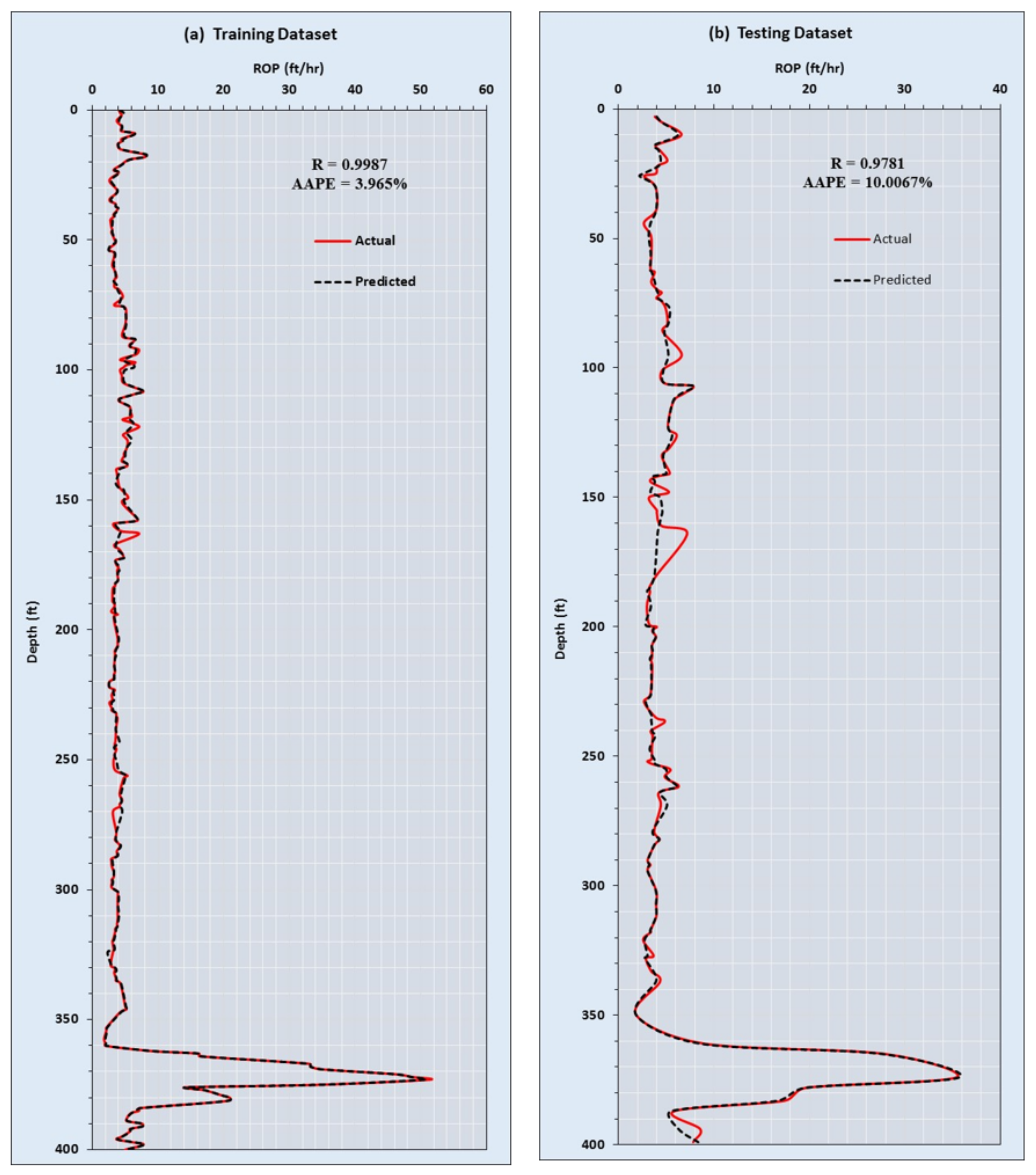
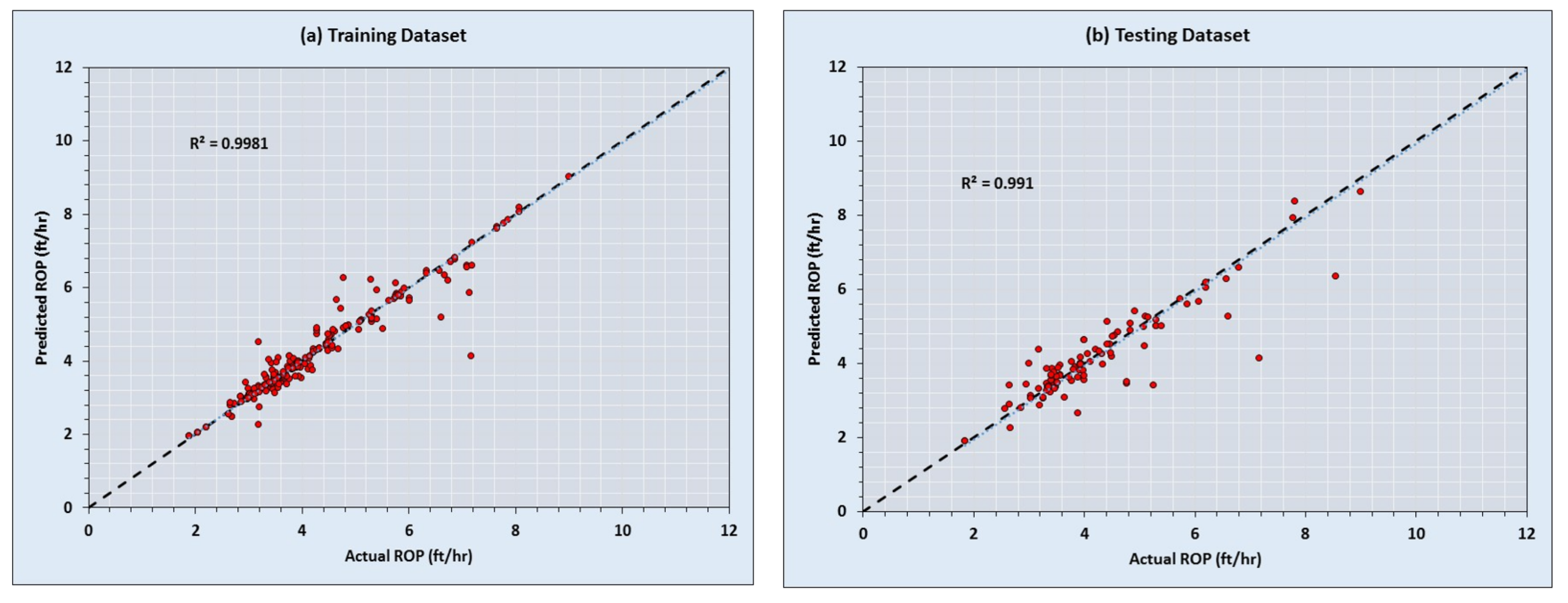
When 70% of the data were used for training, if the actual values of rate of penetration are compared with the predicted ones, ANN was found to estimate ROP with R = 0.999 and AAPE = 3.965% as shown in Figure 2a. Comparing the predicted ROP values and the actual values, the training results have a coefficient of determination (R²) of 0.998 as shown in Figure 3a.

Likewise, 30% of the data were used for model testing. The artificial neural network (ANN) was able to estimate ROP with R = 0.978 and AAPE = 10.0% as shown in Figure 2b. The predicted values compared to the actual values with the coefficient of determination (R²) of 0.991 as shown in Figure 3b.

3.1. New Model Equation

A novel correlation was derived from the ANN model using the biases and weights of neurons-connections among input, hidden and output layers. The new ROP correlation is shown in the following Equation (6):

$$RO{P}_n=\left[{\displaystyle \sum }_{i=1}^N{w}_{2i} \left(e^{-{\left(w_1{}_{i,1}WOB+w_1{}_{i,2}SPP+w_1{}_{i,3}RPM+ w_1{}_{i,4}Q+ w_1{}_{i,6}\tau +w_1{}_{i,5}{\rho }_m+w_1{}_{i,7}{V}_F+ w_1{}_{i,8} V_p+ w_1{}_{i,9}{Y}_p+w_1{}_{i,10}\delta +b_1{}_i\right)}^2 }\right)\right]+b_2$$

(6)

where ROP is the rate of penetration (ft/hr), N is the neuron number, ${\mathrm{w}}_2{}_{\mathrm{i}}$ is the weight connected the hidden with the output layers, ${\mathrm{w}}_1{}_{\mathrm{i}}$ is the weight connected the input with the hidden layers. WOB is weight on bit (klb), SPP is the stand pipe pressure (psi), RPM is rotation per minute (rpm), Q is flow pump rate (gpm), τ is drilling torque (klb_f), ρ_m is mud density (PCF), V_F is funnel viscosity (cP), V_p is plastic viscosity (cp), Y_p is yield point $\left(\frac{\mathrm{lb}}{100{ \mathrm{ft}}^2}\right)$, $\mathsf{\delta }$ is solid (%), b₁ is the bias in the hidden layer and b₂ is the bias in the output layer. The biases and weights of the ANN ROP model are presented in

Table 8. The Biases and Weights of the developed ANN equation for ROP prediction.

N	W1										b1	W2	b2
1	1.963	1.606	0.190	−1.086	2.265	3.591	−1.537	0.494	0.264	−0.299	−0.482	−1.100	−0.2771
2	−0.997	−0.781	−2.622	−1.960	0.964	0.548	−0.474	−0.296	−1.392	−0.186	0.957	1.749
3	0.994	−0.057	1.931	0.675	−1.108	−0.520	−0.425	−0.245	0.539	0.914	0.002	1.895
4	−1.278	2.401	−1.756	−0.509	−0.226	0.276	−1.926	−0.037	0.154	−0.168	0.790	−2.568
5	−1.545	−0.316	−0.229	−2.798	−3.364	1.088	0.628	0.000	−0.542	0.583	0.678	−2.333
6	−1.813	1.722	−1.778	−1.265	−1.439	−0.861	−2.019	0.116	−0.151	1.510	1.209	3.110
7	−0.899	0.836	1.285	1.015	−0.009	−0.113	0.688	−0.603	0.243	−0.478	0.360	−2.347
8	1.231	−0.300	−1.112	−1.771	1.712	1.830	−0.277	−0.472	−0.288	−0.443	1.017	1.764
9	−0.883	−1.554	−1.020	−0.291	0.136	0.408	−0.273	2.636	1.084	0.735	2.982	−1.703
10	−0.440	−0.520	0.345	−0.523	−0.666	1.764	0.087	−0.682	−0.039	−0.271	0.236	2.643
11	1.916	−0.489	0.131	1.672	2.251	0.007	−2.295	0.788	1.580	1.177	−0.409	2.909
12	0.405	−0.339	0.238	−0.170	2.668	−0.237	−0.189	−0.332	0.420	−1.401	−0.155	−2.644
13	−1.404	1.063	−1.608	−1.175	0.097	2.101	−0.301	0.713	1.206	−0.586	0.757	−1.425
14	1.093	−0.610	−0.699	0.060	0.012	1.992	0.111	0.506	0.270	0.197	0.270	−1.801
15	−0.629	1.044	−0.409	0.686	−0.261	1.162	−1.618	−0.467	0.288	0.863	0.084	3.079
16	1.295	0.345	1.300	−0.765	−3.459	−0.373	1.710	−0.686	0.628	1.878	0.192	−2.233
17	1.196	0.416	−0.915	−0.547	1.567	2.744	−0.239	−1.310	−0.384	−0.105	−0.014	1.712
18	−1.234	0.349	−0.535	0.697	−0.005	0.669	1.657	−0.441	−0.125	−1.670	0.197	−3.105

N = Hidden Layer Neurons. W1 = Weight between Inputs and Hidden Layer. b1 = Hidden Layer Biases. W2 = Weight between Output and Hidden Layer. b2 = Output Layer Biases.

.

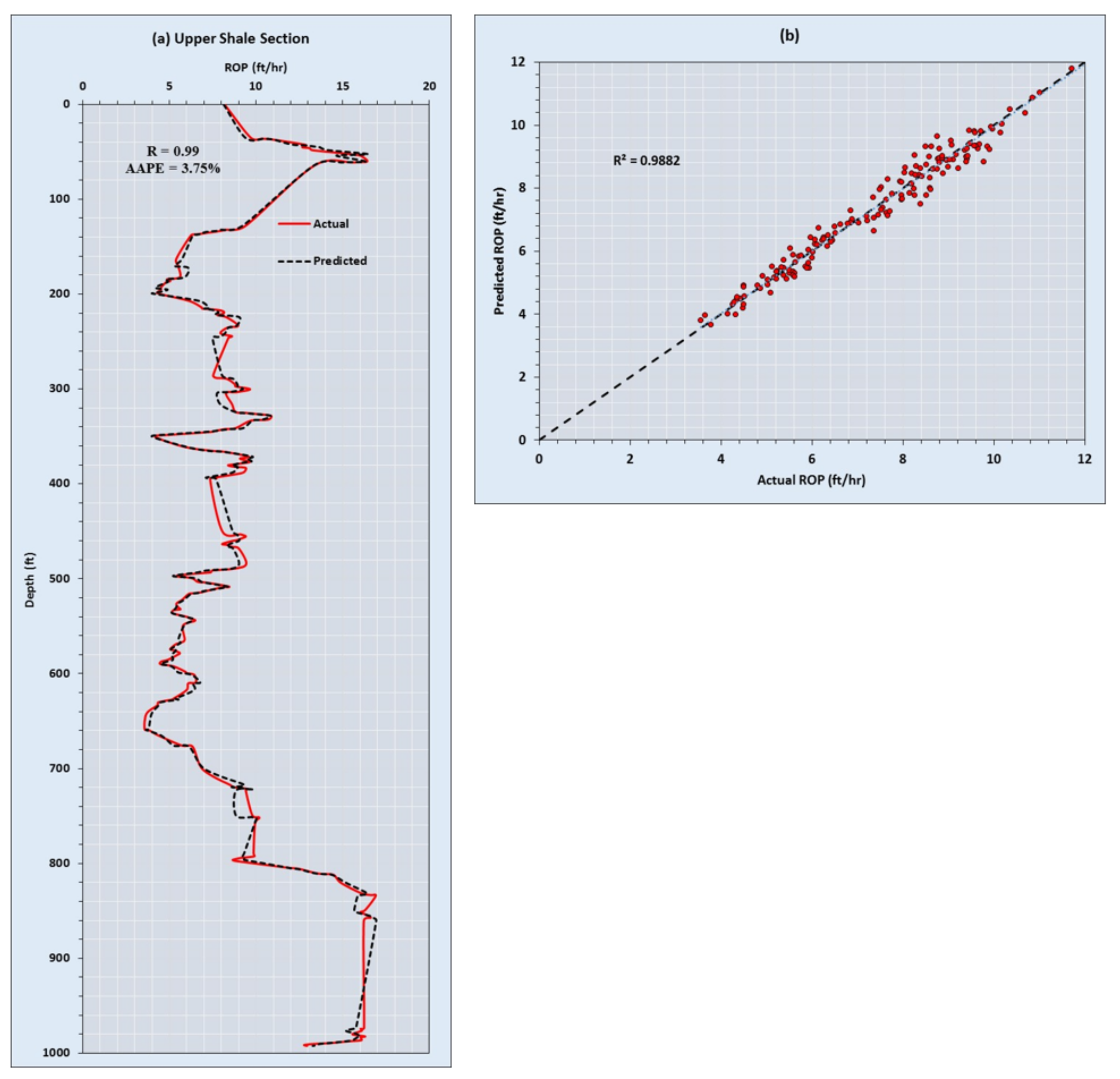
A new data set (200 data points) was collected from an upper shale section (1000 ft) in the same well which was never used while building and testing the ANN model. ROP ranged from 3.5 to 16.9 ft/h and the other input parameters were in the same range as the training data for the ROP model.

It is clear from Figure 4a that the developed correlation for ROP prediction, Equation (6) was able to predict the ROP with a high accuracy where the average absolute error was 3.57% and the correlation coefficient was 99%. Figure 4b shows that the coefficient of determination was 0.988 for the new set of data using the developed ROP empirical correlation.

3.2. Comparison with Empirical Models

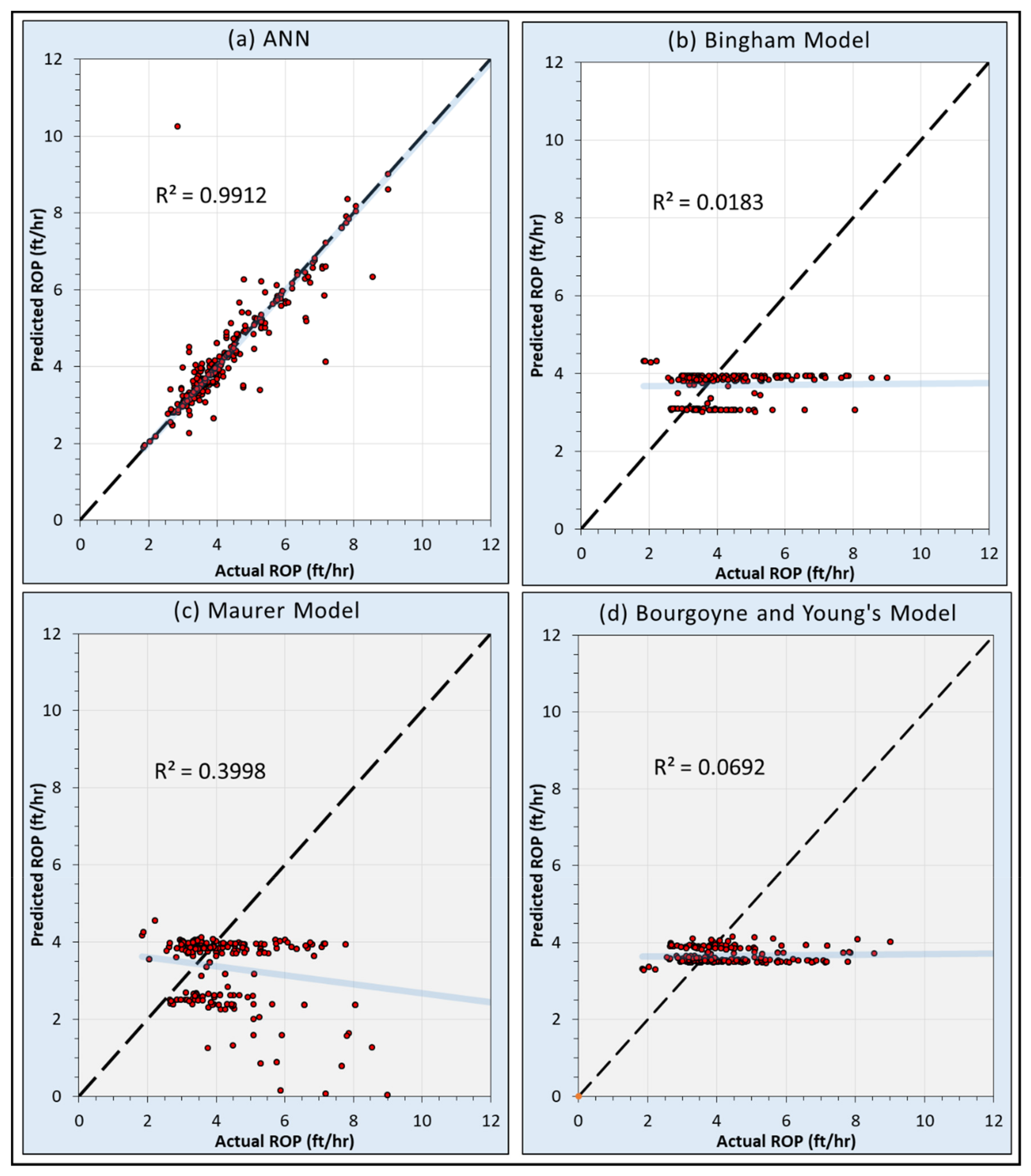
For further verification of the new model equation, we compared it with three empirical ROP models such as Maurer, Bingham and Bourgoyne & Young’s. By applying ANN on the whole dataset, (R = 0.996), (APPE = 5.776%) and (R² = 0.991) were achieved as shown in Figure 5a and Figure 6a.

Bingham model is an empirical model with two constants, drillability (k) and bit weight (a₅). Therefore, we performed a regression analysis to compute k and a₅. Based on the regression analysis of the study dataset k was 0.0437 and (a₅) was 0.0001. Using the Bingham model to predict ROP resulted in a low R of (0.137) and a high AAPE of 25.56% between the predicted and the actual ROP values as shown in Figure 5b. Likewise, the coefficient of determination (R²) was very low (0.0183) as shown in Figure 6b.

Similarly, we performed a regression analysis to calculate the constant (k) for the Maurer model (k = 4,695,629.65). Maurer model predicted ROP with relatively low R (0.631) and high AAPE (23.14%) as shown in Figure 5c. The coefficient of determination (R²) between predicted and actual ROP values was 0.3998 as shown in Figure 6c.

The multi-regression analysis was performed to calculate all (a) constants for Bourgoyne and Young’s empirical model. The (a) constants were found to be as follow:

$$a_1=1.488, a_2=0.4\times {10}^{-6}, a_3=-0.3\times {10}^{-6}, a_4=0.2\times {10}^{-7},$$

$$a_5= -4.6\times {10}^{-2}, a_6= -3.2\times {10}^{-1},a_7= 3.937, a_8=0.448$$

Bourgoyne & Young’s model was used to estimate ROP with a low R of 0.263 and a high AAPE of 23.66% as shown in Figure 5d. The model values of rate of penetration and the actual value have a coefficient of determination (R²) equal to 0.0692 as shown in Figure 6d.

Results of comparing the new model equation and the three empirical published models are summarized in

Table 9. Comparison between the new ANN Model and the published Models.

Method	R	AAPE	R2
New ANN-Based Equation	0.996	5.776	0.9912
Bingham Model	0.137	25.564	0.0183
Maurer Model	0.631	32.139	0.3998
Bourgoyne and Young’s Model	0.263	23.663	0.0692

. The statistics show that the new ANN-based model equation outperformed the above previous empirical equations as indicated by the high correlation coefficient, low AAPE, and high R² compared to those of the published model.

4. Conclusions

Rate of penetration was predicted by the artificial neural network (ANN) using real filed data set in the deep shale formation. The following points can be concluded from the obtained results:

➢

Real drilling surface parameters and drilling fluid properties are very significant and should be considered in the estimation of penetration rate for shale formation.

➢

ANN penetration rate model was based on five real drilling surface parameters (WOB, RPM, ROP, T, and Q) and five drilling fluid properties (MW, PV, FV, YP, and Solid %).

➢

ANN-ROP model is able to estimate the rate of penetration with a high accuracy (R = 0.996, AAPE = 5.77% and R² = 0.99).

➢

ROP penetration rate model outperformed the common penetration rate models by its simple prediction of ROP. It is able to estimate the ROP in a short time with high accuracy compared to Bingham, Maurer and Bourgoyne & Young’s model models which require a lot of calculations and produced lower accuracy.

The applicability of the proposed ANN model depends on the range of the data. For any data, that has the same range of the input data in Table 1 or close to this range, can be implemented in the developed model to predict the ROP with reasonable accuracy. Formation properties are also major parameters that need to be considered to predict the ROP. However, the effects of formation properties were included indirectly by incorporating the ROP with the other real drilling surface parameters such as torque.

References

- Bourgoyne, A.T.; Millheim, K.K.; Chenevert, M.E.; Young, F.S. Applied Drilling Engineering; Richardson, T.X., Ed.; Society of Petroleum Engineers: Houston, TX, USA, 1986; Volume 1. [Google Scholar]
- Bahari, A.; Baradaran Seyed, A. Trust-Region Approach to Find Constants of Bourgoyne and Young Penetration Rate Model in Khangiran Iranian Gas Field. In Proceedings of the SPE-107520-MS Was Presented at Latin American & Caribbean Petroleum Engineering Conference, Buenos Aires, Argentina, 15–18 April 2007. [Google Scholar] [CrossRef]
- Akgun, F. How to Estimate the Maximum Achievable Drilling Rate without Jeopardizing Safety. In Proceedings of the SPE-78567-MS Was Presented at Abu Dhabi International Petroleum Exhibition and Conference, Abu Dhabi, UAE, 13–16 October 2002. [Google Scholar] [CrossRef]
- Elkatatny, S.M.; Tariq, Z.; Mahmoud, M.A.; Al-AbdulJabbar, A. Optimization of Rate of Penetration using Artificial Intelligent Techniques. In Proceedings of the ARMA-2017-0429 Was Presented at 51st U.S. Rock Mechanics/Geomechanics Symposium, San Francisco, CA, USA, 25–28 June 2017. [Google Scholar]
- Hossain, M.E.; Al-Majed, A.A. Fundamentals of Sustainable Drilling Engineering; Scrivener Publishing LLC: Beverly, MA, USA, 2015. [Google Scholar]
- Maurer, W. The Perfect—Cleaning Theory of Rotary Drilling. J. Pet. Technol. 1962, 14, 1270–1274. [Google Scholar] [CrossRef]
- Bingham, M.G. A New Approach to Interpreting—Rock Drillability; Petroleum Pub. Co.: Tulsa, OK, USA, 1965. [Google Scholar]
- Bourgoyne, A.T.; Young, F.S. Multiple Regression Approach to Optimal Drilling and Abnormal Pressure Detection. J. SPE 1974, 14, 371–384. [Google Scholar] [CrossRef]
- Warren, T.M. Penetration-Rate Performance of Roller–Cone Bits. SPE Drill. Eng. 1987, 2, 9–18. [Google Scholar] [CrossRef]
- Hareland, G.; Hoberock, L.L. Use of Drilling Parameters to Predict In-Situ Stress Bounds. In Proceedings of the SPE-25727-MS Was Presented at the SPE/IADC Drilling Conference, Amsterdam, The Netherlands, 22–25 February 1993. [Google Scholar] [CrossRef]
- Zare, J.; Shadizadeh, S.R. Managed Pressure Drilling to Increase Rate of Penetration and Reduce Formation Damage. Pet. Sci. Technol. 2014, 32, 1833–1842. [Google Scholar] [CrossRef]
- Van Der Aalst, W.M.P.; Rubin, V.; Verbeek, H.M.W.; Dongen, B.F.V.; Kindler, E.; Günther, C.W. Process mining: a two-step approach to balance between underfitting and overfitting. Softw. Syst. Model. 2008, 9, 87–111. [Google Scholar] [CrossRef]
- Ahmed, A.; Elkatatny, S.; Ali, A.; Mahmoud, M.; Abdulraheem, A. New Model for Pore Pressure Prediction While Drilling Using Artificial Neural Networks. Arabian J. Sci. Eng. 2018, 44, 6079–6088. [Google Scholar] [CrossRef]
- Haykin, S.; Hakin, S. The Neural Networks a Comprehensive Foundation; Macmillan College Publishing Company: Stuttgart, Germany, 1998. [Google Scholar]
- Khalil-Hani, M.; Liew, S.S.; Bakhteri, R. An Optimized Second Order Stochastic Learning Algorithm for Neural Network Training. Neural Inf. Proc. Lect. Notes Comput. Sci. 2015, 38–45. [Google Scholar] [CrossRef]
- Bilgesu, H.I.; Tetrick, L.T.; Altmis, U.; Mohaghegh, S.; Ameri, S. A New Approach for the Prediction of Rate of Penetration (ROP) Values. In Proceedings of the SPE-39231-MS Was Presented at SPE Eastern Regional Meeting, Lexington, KY, USA, 22–24 October 1997. [Google Scholar] [CrossRef]
- Moran, D.P.; Ibrahim, H.F.; Purwanto, A.; Osmond, J. Sophisticated ROP Prediction Technology Based on Neural Network Delivers Accurate Results Sophisticated ROP. In Proceedings of the SPE-132010-MS Was Presented at IADC/SPE Asia Pacific Drilling Technology Conference and Exhibition, Ho Chi Minh City, Vietnam, 1–3 November 2010. [Google Scholar] [CrossRef]
- Jahanbakhshi, R.; Keshavarzi, R.; Jafarnezhad, A. Real-time Prediction of Rate of Penetration during Drilling Operation in Oil and Gas Wells. In Proceedings of the ARMA-2012-244 Was Presented at 46th U.S. Rock Mechanics Geomechanics Symposium, Chicago, IL, USA, 24–27 June 2012. [Google Scholar]
- Arabjamaloei, R.; Shadizadeh, S. Modeling and Optimizing Rate of Penetration Using Intelligent Systems in an Iranian Southern Oil Field (Ahwaz Oil Field). Pet. Sci. Technol. 2011, 29, 1637–1648. [Google Scholar] [CrossRef]
- Bataee, M.; Mohseni, S. Application of Artificial Intelligent Systems in ROP Optimization: a Case Study. In Proceedings of the SPE-140029-MS Was Presented at SPE Middle East Unconventional Gas Conference and Exhibition, Muscat, Oman, 31 January–2 February 2011. [Google Scholar] [CrossRef]
- Khoukhi, A.; Ibrahim, A. Rate of Penetration Prediction and Optimization using Advances in Artificial Neural Networks, a Comparative Study. In Proceedings of the 4th International Joint Conference on Computational Intelligence, Barcelona, Spain, 5–7 October 2012. [Google Scholar] [CrossRef]
- Shi, X.; Liu, G.; Gong, X.; Zhang, J.; Wang, J.; Zhang, H. An Efficient Approach for Real-Time Prediction of Rate of Penetration in Offshore Drilling. Math. Prob. Eng. 2016, 2016, 1–13. [Google Scholar] [CrossRef]
- Jiang, W.; Samuel, R. Optimization of Rate of Penetration in a Convoluted Drilling Framework using Ant Colony Optimization. In Proceedings of the SPE-178847-MS Was Presented at IADC/SPE Drilling Conference and Exhibition, Fort Worth, TX, USA, 1–3 March 2016. [Google Scholar] [CrossRef]
- Manshad, A.; Rostami, H.; Toreifi, H.; Mohammadi, A. Optimization of Drilling Penetration Rate in Oil Fields Using Artificial Intelligence Technique. In Heavy Oil: Characteristics, Production and Emerging Technologies; Nova Science Publishers: Hauppauge, NY, USA, 2017; pp. 255–269. [Google Scholar]
- Ahmed, O.; Adeniran, A.; Samsuri, A. Rate of Penetration Prediction Utilizing Hydromechanical Specific Energy. In Drilling; BoD—Books on Demand: Berlin, Germany, 2018. [Google Scholar] [CrossRef]
- Bodaghi, A.; Ansari, H.R.; Gholami, M. Optimized support vector regression for drilling rate of penetration estimation. Open Geosci. 2015, 7. [Google Scholar] [CrossRef] [Green Version]
Figure 1.
Architecture of the backpropagation using an artificial neural network (ANN) model.
Figure 2.
Statistics of training (a) and testing (b) ANN model results, depth refers to the top and the bottom of the deep shale formation. Note: The data range of testing data subset is within the range of the training data subset.
Figure 3.
Scatter diagram comparing the predicted rate of penetration (ROP) values and actual values for training (a) and testing (b) datasets.
Figure 4.
New data set from the upper shale section for model validation.
Figure 5.
The new ANN model in comparison with three published empirical models. (a). New ANN-Based Equation, (b). Bingham Model, (c). Maurer Model, and (d). Bourgoyne and Young’s Model.
Figure 6.
Scatter diagram comparing predicted ROP values and actual values for the new ANN model and the three published empirical models.