Combined Experimental and Field Data Sources in a Prediction Model for Corrosion Rate under Insulation


1
School of Engineering, Faculty Science and Technology, Quest International University Perak, Ipoh 30250, Perak, Malaysia
2
Mechanical Engineering Department, Universiti Teknologi PETRONAS, Sri Iskandar 31750, Perak, Malaysia
3
Electrical and Electronics Engineering Department, Universiti Teknologi PETRONAS, Sri Iskandar 31750, Perak, Malaysia
*
Author to whom correspondence should be addressed.
Sustainability 2019, 11(23), 6853; https://0-doi-org.brum.beds.ac.uk/10.3390/su11236853
Submission received: 8 September 2019
/
Revised: 26 October 2019
/
Accepted: 9 November 2019
/
Published: 2 December 2019
(This article belongs to the Section Sustainable Engineering and Science)
Abstract
:Corrosion under insulation (CUI) is one of the increasing industrial problems, especially in chemical plants that have been running for an extended time. Prediction modeling, which is one of the solutions for this issue, has attracted increasing attention and has been considered for several industrial applications. The main objective of this work was to investigate the effect of combined data input in prediction modeling, which could be applied to improve the existing CUI rate prediction model. Experimental data and field historical data were gathered and simulated using an artificial neural network separately. To analyze the effect of data sources on the final corrosion rate under the insulation prediction model, both sources of data from experiment and field data were then combined and simulated again using an artificial neural network. Results exhibited the advantages of combined input data type from the experiment and field in the final prediction model. The model developed clearly shows the occurrence of corrosion by phases, which are uniform corrosion at the early phases and pitting corrosion at the later phases. The prediction model will enable better mitigation actions in preventing loss of containment due to CUI, which in turn will improve overall sustainability of the plant.
1. Introduction
Corrosion under insulation (CUI) refers to external corrosion on the surface of piping and/or vessels fabricated from low alloys, carbon manganese steel, or austenitic stainless steel that happens beneath insulation due to the penetration of water. CUI is typically localized corrosion but is difficult to identify because it is hidden under insulation material until it becomes a serious problem, which especially occurs in chemical plants that have been running for an extended time [1].
The CUI problem in industries increases with years. As had been reported by Exxon Mobile Chemical and National Association of Corrosion Engineers (NACE), the utmost incidence of leakages in the refining and chemical industries is due to corrosion under insulation (CUI) and out of 30 facilities, 17 state CUI as the focal challenge in their industries [2]. CUI also has a high implication to financial cost. The United States Congress reported that direct loss and maintenance costs due to corrosion are approaching $276 billion per year, where practically 40% to 60% of maintenance costs are allocated for CUI piping detection and rectification of CUI occurrence [3,4]. This value would be twice if indirect costs were considered. Likewise, the NACE Corrosion Costs Study stated that corrosion costs in the United States are approaching $1 trillion annually and are estimated to exceed this amount in a couple of years [5]. In addition to important CUI detection methods for prevention and inspections, it is also very important to have a high-accuracy CUI prediction model as a guideline to schedule effective maintenance planning to avoid higher costs due to CUI.
Over the past few years, prediction modeling has attracted increasing attention and has been considered for applications in several industries, including for cases such as corrosion in piping [6,7,8]. The current standards for CUI prediction, such as in API 581, are developed based on experimental and/or numerical works, which are sometimes generalized and contain flaws [9]. At present, numerous prediction models for CUI have been developed using historical field data as data input on each local industry or country [10]. Although this type of data input is well established for enabling the development of different places of corrosion under the insulation model to be used as a local maintenance guide, the data input effects on the available model have not been extensively studied. Some research has been reported without the changing behavior of the corrosion phase, as the historical field data was only collected after decades of operation [11,12]. This issue affects the practicality and the quality of the prediction model developed.
Therefore, a substantial study on the type of data input required for developing a prediction model is essential to understand the relative importance of combined data input in the CUI prediction model. In this work, the single data input, from historical field data and experimental data explicitly, and combined data input of both field and experimental data are tested to investigate the effect of type of data input on the CUI prediction model.
2. Materials and Methods
2.1. Historical Field Data Input
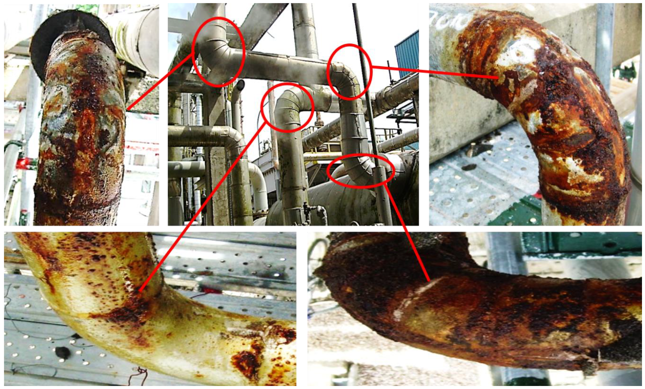
The historical field data was initially collected from three gas processing plants (GPP) with a total of 11,000 m of pipe length on the east coast of the Malaysia Peninsular (5°50′30” N, 104°07′3, 7′30” E) near the South China Sea which experiences equatorial climate. Both visual inspection data and wall thickness data types were involved in the historical field data collection after the removal of insulation on the piping surface. In visual inspection data, CUI data were treated as binary data. When CUI was found, data was denoted as 1, and 0 when CUI was not found. An example of visual inspection data collected from the field where CUI was heavily detected is shown in Figure 1.
For wall thickness data, the detailed value for nominal thickness, Nt in millimeters, and actual thickness (average wall thickness), At in millimeters, and year in service denotes by Yrservice were recorded to calculate the field CUI rate, CRf in mm/year as given in Equation (1).
Other than that, the field data were configured and classified for each parameter which involves the six groups of operating temperature (less than −12 °C, −12 °C to 16 °C, 17 °C to 48 °C, 49 °C to 93 °C, 94 °C to 121 °C, and above than 121 °C) as prescribed in API 581 practices, age of the pipe (15 to 20 years of pipe age), type of insulation (cellular glass, calcium silicate, perlite and rockwool), design of pipe (with elbow or no elbow in pipe design), pipe material (carbon steel or stainless steel), and small (less than 2 inches pipe diameter) or big bore pipe (more than 2 inches pipe diameter).
For field data analysis and simulation, the CUI data recorded were then compared with the plant design and operating data to ensure the CUI collected data were satisfactory for further analysis. Data were tabulated and analyzed using pivot table functions in Microsoft Excel.
As the input data from the field were still limited in generating an effective final CUI prediction model, results obtained were simulated through the prediction profiler simulator function in Statistical Discovery JMP 10.0 2012 SAS Integration 9.1.3 Server software package. The steps are simplified as:
- (1)
- Determination of artificial neural network (ANN) parameters: Available parameters were operating temperature (°C), insulation type, pipe design, piping thickness (mm), type of pipe material, type of environment (weather condition either rainy or sunny), elapsed time (years), and CUI rate (mm/year) data. This surface profiler is suitable when the data contain more than one continuous factor. In this study, the operating temperature and corrosion rate were set as a continuous factor.
- (2)
- Definition of ANN architecture: The basic structure of the ANN was identified and determined. The layer of hidden nodes, the input parameter, and the output parameter were clearly prescribed. For this study, one hidden layer was used, and a hyperbolic tangent function (TanH) with a sigmoid type was used as an activation function for the ANN test.
- (3)
- Data normalization, filtration, and initialization: Field data collected from the actual plant in Kerteh, Malaysia, were simulated. Before that, the incomplete, missing information from the database or outlier values were removed to ensure only significant data were included. Usually, the field data are collected without the thickness measurement. Thus, data were simulated to generate sufficient data to continue with normalization and filtration. During this process, the range of CUI rate data was set from 0 to 1 mm/year based on ABB EUT.249A references as a common CUI rate occurrence [13].
- (4)
- ANN training and surface profiling: For training purposes, 70% of normalized data was used, while 15% for validation set and other 15% were for testing the basic model being developed. The surface profiling platform was used to plot points on the surface model after the ANN training completed. The points were selected based on the parameter and profiled the loss as a function of the parameters. The CUI rates were determined and tabulated in Excel sheets or in graphs.
2.2. Experimental Work Data Input
There were two phases during the experimental work. The initial phase embraced the preparation, setup, testing, and calibration of the entire probe for the CUI experiment based on the Official Guide for Laboratory Experiment of Corrosion under Insulation (ASTM G198-07) specification, while the second phase was the modified experiment which is suited to the main parameters from the historical field data analysis [14]. Three main items, the insulation, rings specimen, and the solution reservoir, were properly prepared.
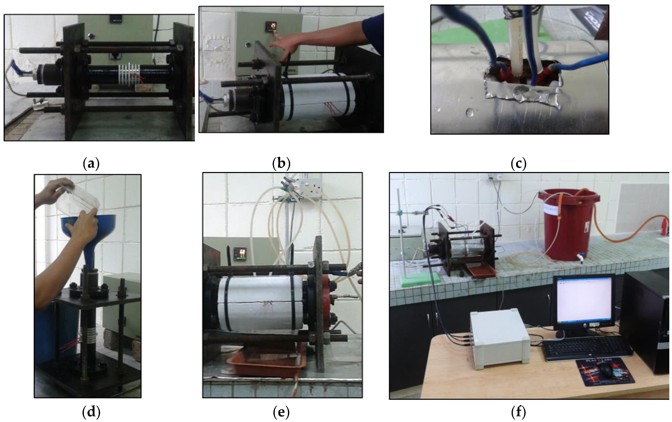
The Perlite insulation in the initial phase was prepared according to ASTM G189-07, while in the modified phase, calcium silicate insulation (2.5-inch outside diameter and 1.6-inch thickness) was placed around the testing section to provide the annular space to retain the test environment, as shown in Figure 2a.
For the rings specimen, a piping material of carbon steel grade A106B, density 7.86 g/cm³ with a 2-inch diameter, 0.2-inch thickness, and specimen area of 9.58 cm³ was used for both phases. Each ring specimen was surface finished, ground to 600 grit, soaked into a chemical cleaning solution which contained 1000 mL hydrochloric acid (HCl sp. Gr. 1.19), 20 g antimony trioxide (Sb2O3) and 50 g stannous chloride (SnCl2), and placed in an ultrasonic cleaning machine, S30H Elmasonic. The cleaning process was set to 3 min per specimen and dried using a dryer to ensure no pits or particles occurred on the rings’ surfaces and weighted as initial mass to the nearest 0.1 mg according to the ASTM Practice G1-03. The ring specimens acted as test electrodes in two separated electrochemical cells, by a dam (bigger Teflon ring of 3.0 inch outside diameter) as presented in Figure 2b,c. The Teflon spacers were machined from the same spacer material, polytetrafluoroethylene (PTFE) resins. During the experiment, the carbon steel rings separated by Teflon spacers were held by blind flange pipe sections on both ends, as in Figure 2d.
The solution reservoir is the solution that represents an atmospheric condensate with impurities of acids and chlorides found in industries. The solution made contained 100 ppm NaCl dissolved in reagent water and 1 M of sulfuric acid, H2SO4, with pH 6. The flow of this solution was controlled by a micro-metering pump with a maximum capacity of 30 mL/min and a maximum stroke frequency of 300 strokes per minute. The pumping flow rate was tested and stabilized until the dropped solution was 5 mL/min with 14 strokes per minute. For one accelerated CUI experiment (accelerating the corrosion process), the wet and dry condition was controlled with a duration of 20 h wet and 4 h dry for each cycle minimum for 72 h continuously. The benefit of the accelerated CUI experiment, especially to study the performance of the CUI rate regarding the time elapsed, can be found in [15].
In the completed CUI cell run, both electrochemical cells comprised three (3) rings specimens. The center ring was used as the working electrode (WE), while the other two rings were used as the reference electrode (RE) and auxiliary electrode (AE) connected to a potentiostat, as in Figure 3a,c. The ring specimens acted as test electrodes in two separate electrochemical cells and were monitored by a Gill AC-1493 Sequencer software package specifically for the linear polarization resistance (LPR) function. The LPR function was used because it responded fast and could detect the changes in the corrosion rate during the experiment in minutes.
As the CUI cell experiment should simulate the real field condition, the internal piping condition was filled with the synthetic oil, immersion heater, and temperature controller, as in Figure 3c,d. After the CUI cell and insulation was completed, as presented in Figure 3b, the cyclic temperature was set at 65 °C during wet conditions and 121 °C during dry conditions and the solution representing the environment condition which was dropped from the solution tank through a valve and solution inlet, continued to drain at the bottom as in Figure 3e,f. After the CUI test was finished within the specified exposure time, the insulation was dismantled, and the ring specimens were cleaned and weighed carefully after exposure, using the standard specifications mentioned in ASTM G1-03, previously.
Three (3) replicates were used for each test and recorded. For each experimental replicate, six (6) samples were produced, and the average values of mass loss were calculated. For the experimental CUI rate in millimeters per year, the CRexp of each sample was calculated using the relationship in Equation (2).
where K is constant (8.76 × 104 mm/yr). This K value in millimeters per year was selected beyond the several other unit choices to express corrosion rates, as mentioned in ASTM G1-90, to ensure the standardization of the results from the experiment can be directly compared with the results from the field which were gathered in millimeters per year. M is a mass loss in grams, A is an exposed area in centimeters squared, T is a time of exposure in hours, and density, D, in centimeters cubed. Similarly to the field, as the input data from the experiment were still limited in generating an effective final prediction model, results obtained were also simulated through the prediction profiler simulator function in the Statistical Discovery JMP 10.0.0 2012 SAS Integration 9.1.3 Server software package. The same steps can be referred to in Section 2.1.
2.3. CUI Rate Prediction Modeling
In developing the final CUI rate prediction model, only the most influential input factors from the field and experiment were included because the process and predictive ability of the artificial neural network (ANN) greatly depends on the best input set. In fact, if the model includes irrelevant variables, the model will be difficult to train, and a less accurate model will be produced. Before this CUI model development, the most influential factors for both field and experimental data were determined [16,17]. Thus, in the final CUI rate model, the data input consisted of the most influential input parameter, which was the operating temperature (℃), with an addition of the age of pipe to ease of time-based measurement. The output was the CUI rate in millimeters per year.
The final CUI rate prediction was modeled by three (3) neural network layers’ structure consisting of two (2) input nodes in the first layer, eight (8) hidden nodes in the second layer, and in the third layer, one (1) output node. The two (2) input units involved elapsed time (years) and operating temperature (℃), while the output was the CUI rate (mm/year). The input was then weighted and associated with the connection to the neuron in the hidden layer; then, the activation function was balanced to yield the output. The activation function at each node spread the value of the weighted input to the weighted output and produced non-linear values with a sigmoidal function with backpropagation [18,19]. This expression is shown as in Equation (3).
The output node, Zk is the output value of current layer k-th neuron, €j is the threshold or bias from the current layer k-th neuron, while wjk is the joiner weight between the maiden layer and forward layer neuron. yj is the input layer value based on the j-th neuron, whereas the effect of €k is an adjustment to the sigmoid function shape. In this study, a sigmoidal function of a hyperbolic tangent (TanH) function as in Equation (4) was adopted to ensure the value of the CUI rate was in a specified range during prediction [19,20].
In this equation, y is a linear combination of the Y parameters. Only positive values of this hyperbolic tangent function were gathered as the CUI rate. There are a total of 9344 data input, 4424 from field data, and 4918 were from experimental data. The finalized model featuring the age of pipe with its CUI rate was visualized in a graph, and the fitting line was calculated. In determining the best model for data fitness, a range of neurons in the hidden layers of the ANN was tested. Neurons with the highest R2 value were selected for model development as it indicates the best fit.
Although neural networks are very flexible with high capability and applied in various fields, they may overfit data. It can fit the data model very well but poorly perform the forecast observations. This phenomenon can be defined by observing the sum of squared error (SSE) and the R2 values. If the R2 shows a high value with high SSE, this means the model might be overfitted. A decent model should have a high R2 value with low SSE. Thus, to avoid the overfitting problem, the bias value was applied to the model variables and used an independent data set to evaluate the predictive power of the model.
Further, during the model development process using the prediction profiler simulator function in the Statistical Discovery JMP 10.0 2012 SAS Integration 9.1.3 Server software package, the original data were separated into parts. A part of a dataset was specified to estimate model parameters, while the other part for checking the predictive capability of the model. The neural network was divided into three sets, which were training data, validation data, and testing data. Training data was used for estimations of model parameters. Validation data for finding the optimal value of the weight and calculates or validates the predictive capability of the model while testing data for independent calculation of the model’s predictive capability.
The expected outcome of the statistical analysis done for the CUI rate model was a trend line with a function of elapsed years in relation to the CUI Rate. The configured trend line, smooth fitting, or quadratic line was fitted. Thus, the more accurate line consisting of a corrosion degradation process was produced by the kernel smoothing line method.
In the kernel smoothing method, each data point in the region was weighted according to its distance from the closest point, k. The points close to k were assigned large weights and points far from k, small weights. Another line trend, such as quadratic or linear function, was fitted into the plotted input variable to the output variable by formerly assigned weightage using weighted least squares. This computation of k was made for every single value. This locally weighted expression delivers an estimation of f(k) for the regression surface at any value k in the specified value of input parameter range, R. To bring out the locally weighted regression, a distance function R was created in the space of the input parameter. As an example, let one input parameter be the Euclidean distance. Then, each input variable was divided by its standard deviation if there were multiple inputs, and then the Euclidean distance was used, and the scale adjusted. Other than that, this method required a weight function and a measurement of region size. However, it is not the intention to formulate these functions. Detail formation of this weight function and determination of region size had been explained in detail by Liu [21] and Cleveland [22].
3. Results
3.1. Historical Field Result
There was a total of 1708 inspections spots in the piping susceptible to CUI. Out of 11,000 m of pipe length being reinsulated, 191 m of pipe length had been cut and replaced with new pipes due to the potential higher risk of CUI. This figure reflects 1.74% of the total pipe length. More than 90% of CUI pipes involved carbon steel pipe, while the highest CUI rate involved calcium silicate insulation. Sixty-six percent of cases involved small bore pipe while the remaining 34% involved big bore pipe. Smaller bore size piping commonly had a higher probability of failing as the pipes have a thinner wall compared to bigger bore.
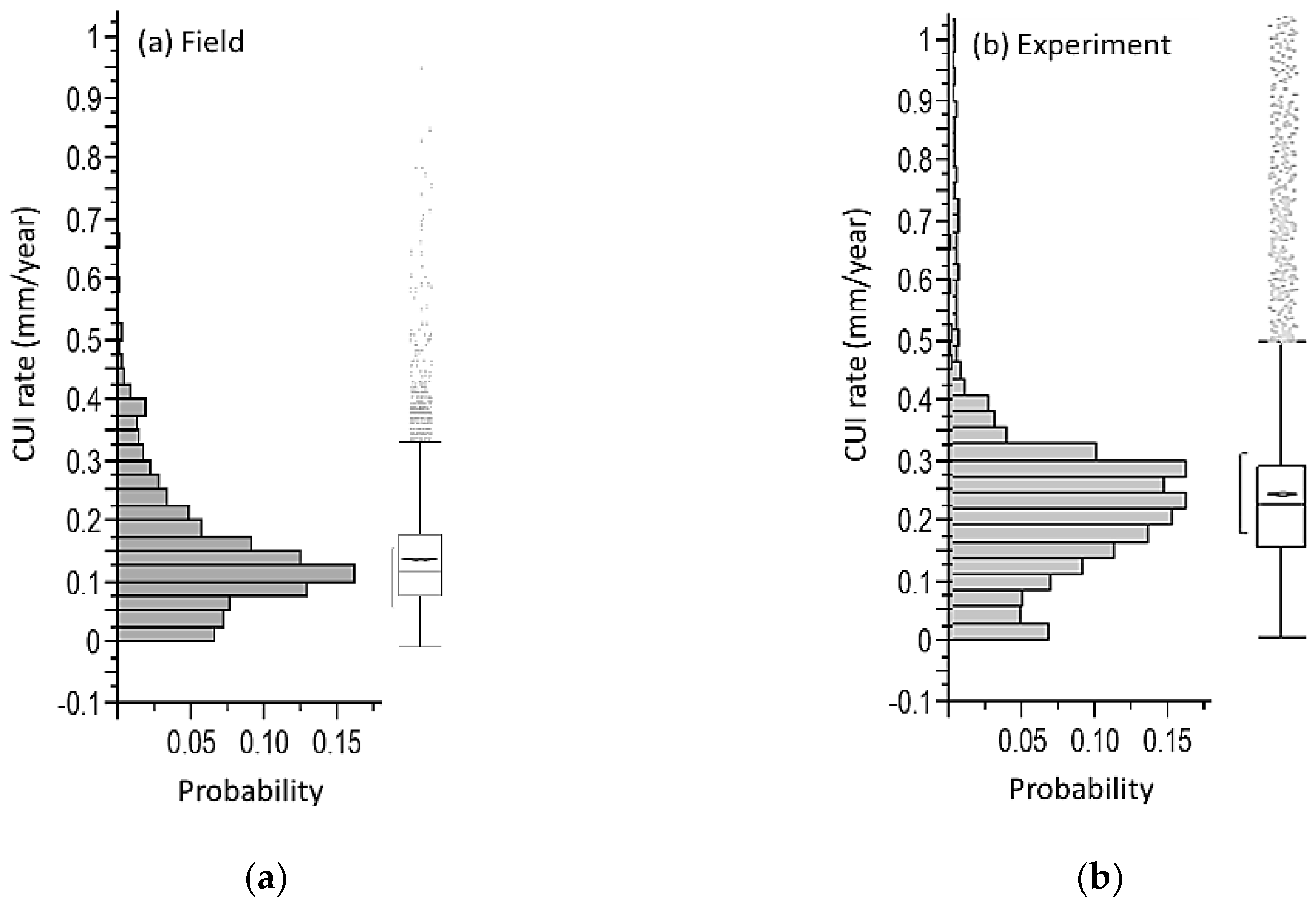
For field data, a total number of 4400 simulated data using statistical analysis software (SAS) for the field with a resulted mean of 0.148 mm/year for the CUI rate, as shown in Figure 4a. The highest CUI rate obtained was 0.957 mm/year, with the median value of 0.124 mm/year, while the lowest value was 0.000 mm/year. Above that, the upper quartile showed a value of 0.187 mm/year, while the lower quartile was 0.083 mm/year. The probability limit values of 95% were 0.151 mm/year for upper and 0.145 mm/year for the lower mean. The low standard deviation of 0.107 and 0.002 mean standard error showed that these empirical field results were dependable for the CUI prediction model development.
The distributional characteristics and the level of the CUI rate in the box plot in Figure 4a show a comparatively short box, which means that the overall CUI rate for the simulated field data has a high level of agreement with each other. These results were also in agreement with the findings in the statistical analysis of the pressure vessel and piping failures by You and Fu [23] and research by Khan et al. [24]. Thus, these CUI impactful parameters from the field were conserved during the experimental work design.
3.2. Experimental Work Result
The results obtained from the experiment were artificially simulated to generate more data using a neural network surface profiler. The distribution of the simulated CUI rate obtained with the probability of occurrence is shown in Figure 4b. The distribution of the CUI rate shows a taller size box plot and whisker, including the outliers, which means the CUI rate held quite different ranges of CUI rate from 0 to 1 mm.
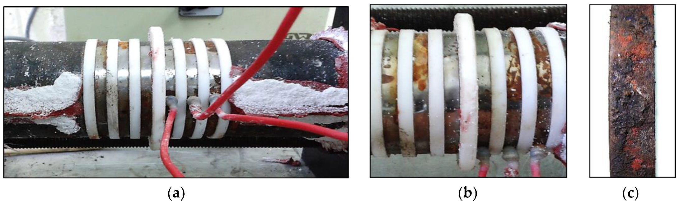
For the quantiles, the maximum rate was 1.169 mm/year, the median value was 0.204 mm/year, while the minimum value was 0.001 mm/year. Other than that, the upper quartile showed a value of 0.263 mm/year, while the lower quartile was 0.137 mm/year. A total number of 4918 simulated data with a mean of 0.222 mm/year for the CUI rate were gained. The CUI rate values of 0.226 mm/year and 0.219 mm/year for lower and upper mean, respectively, show the obtained heuristic results are reliant. The low standard deviation of 0.156 and 0.002 mean standard error shows that the simulated experimental results are reliable for the CUI model development. A glance at some experimental specimen conditions after the insulation was removed is shown in Figure 5a–c.
3.3. CUI Rate Prediction Model
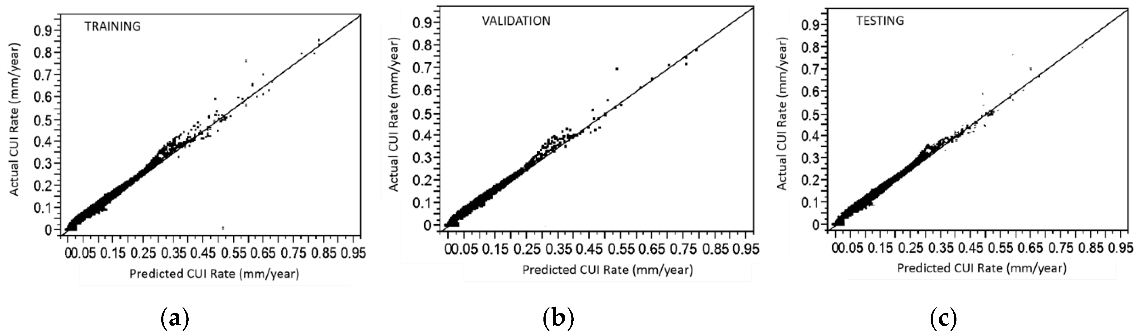
Overall, the R2 value is relatively high, in the range of 0.84 to 0.99, as tabulated in Table 1. The RMSE value is less than 1%, and this indicates that the absolute deviation is acceptable. Based on this, the ideal number of neurons for the hidden layer is 8 nodes with an R2 value of 0.99 and RMSE of 0.009 for training. As for validation and testing, the 8 nodes also gave the best R2 value of 0.90 and 0.91, with the lowest RMSE of 0.010 and 0.009, respectively. This points out that the final CUI rate prediction model developed is reliable.
Other than that, the actual versus predicted graphs for training, validation, and testing for combined data input were produced, as in Figure 6. All graphs show the actual and predicted output fit linearly along the line. This is an indication that the final CUI prediction model developed is consistent.
4. Discussion
4.1. Comparison of Single Type Data and Combined Data in the CUI Rate Model
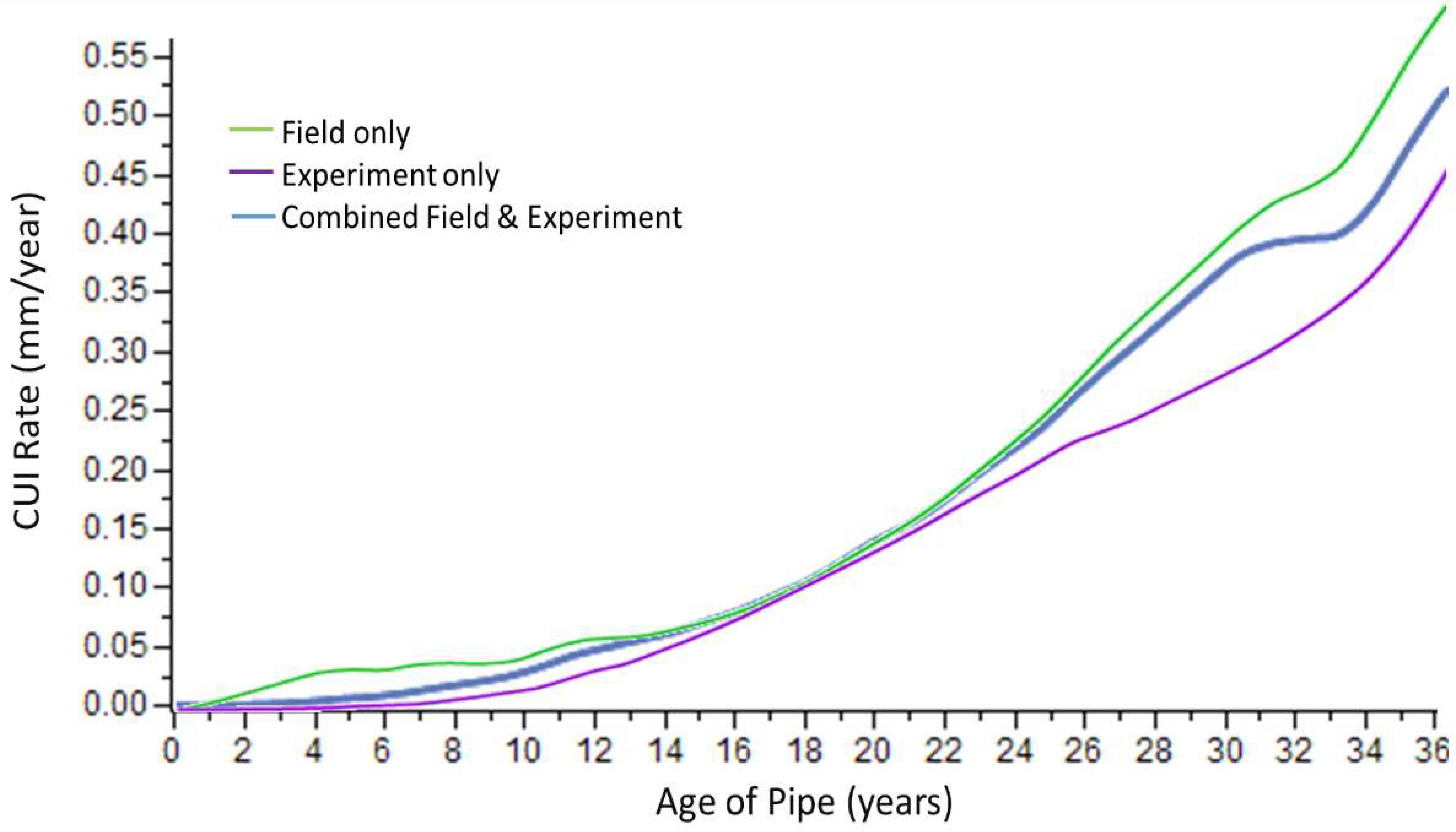
In determining the best model for data fitness, the comparison of single data type and combined data type was done. For single data type, the individual experimental and field result was modeled as output separately. Then, the combined data from experimental and field were model and compared, as in Figure 7.
Based on the comparison model in Figure 7, the experimental results demonstrate much lower corrosion rate values by time, especially after 20 years of time elapsed, which is shown in the yield curve. This prediction might fall into the unhealthy prediction rate for CUI and be dangerous if real piping operation follows this model. Thus, it can be emphasized that the short-term experimental test alone is not reliable for the development of the overall prediction model even though the range of neurons is enough for longer-term prediction as the model predicts lower corrosion loss than actual. However, the importance of this experimental work results is on the initiation part of the corrosion rate model. It shows a more accurate initiation of CUI rate development. Thus, this complements the model made by the field data alone. The model cannot be used to predict the initiation of CUI as opposed to the experimental work. This phenomenon can be understood clearly in Figure 7.
The line model produced by the field data gave high corrosion loss values in the initial phase, although, in actual performance, CUI will not give this corrosion loss as its protective coating and insulation systems are supposedly still active. For this reason, the experimental data were used to complement the model. Despite the roles individually played by the actual field data and experimental data, both are very important. Thus, by integrating and combining both sources of data, the CUI prediction model can be the distinguishing factor in industries since most existing CUI models are dependent on either field or lab work separately. The comparison of the model developed based on single type data, either field or lab, and integration of multi-type data sources was clear.
The smooth line fitting by the combined data sources in blue line, as shown in Figure 7, has a similar trend when associated with the model compiled by Bhandari [10], and then followed the pitting corrosion model trend developed by Melcher for pitting corrosion except for the length of the years elapsed [25]. Even though Fontana [26] did not specify which type of corrosion will occur based on the timeframe, these main types of corrosion due to CUI are still tallied as recorded. For instance, the CUI prediction model consists of the specific elapsed time indicating the association for different phases; this might be considered as an improvement to the existing CUI models available worldwide, which do not embrace the deviations in corrosion mechanism with time. Thus, it can be demonstrated that the corrosion under insulation in oil and gas piping occurs as uniform corrosion in the early phase and at the end, might fail due to the pitting corrosion.
4.2. CUI Rate Model with Corrosion Phases
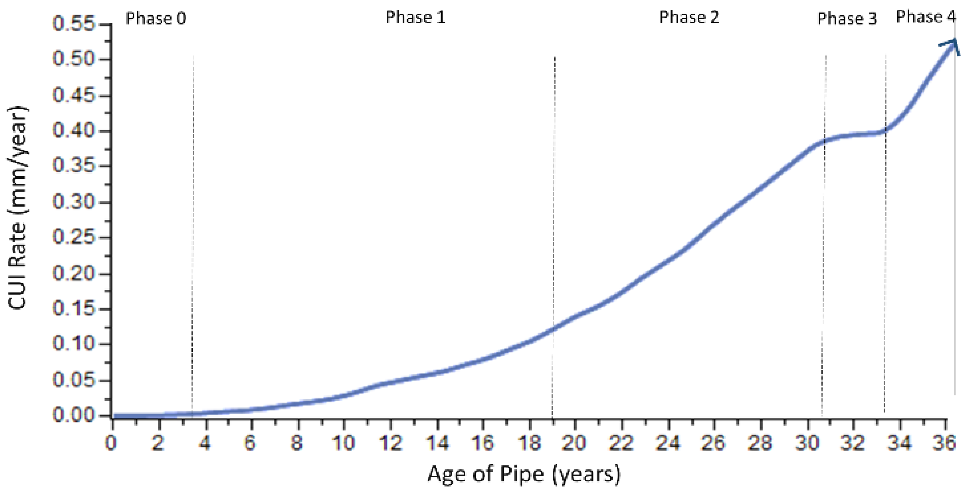
For further analysis, the combined input data for the CUI rate model was divided into several corrosion phases, as shown in Figure 8. Specifically, phase 0 shows a nearly straight line and is linear with a near-zero value. In this phase, the coating and insulation system was in a steady-state and act as a protection system successfully. However, at about 3 years of time elapsed, the protection system might have some trauma, such as the initial degradation of coating materials, slight damage to the insulation, or any other possibility that happens during operation or maintenance. This means that, as time elapsed, local substance reaction can occur unimpeded by the external transmission.
Then, in phase 1 and phase 2, the model can be described in approximation, as an exponential linear relationship between the formation of corrosion and time. If the corrosion has been initiated earlier at the end of phase 0, both of these phases were controlled by the concentration of oxygen in the electrolyte substance. The corrosion rate was administrated by the rate of oxygen content in the chemical reaction, together with the corrosion product layer to the external surface.
However, the linear function in phase 2 will have a higher slope compared to phase 1, as the rate of oxygen diffusion to the corroding surface was increased by time. After the corrosion yields took place on the external surface of the piping material (at the end of phase 2), oxygen flux will decay. During this period, the transition from phase 2 to phase 3, the function will be non-linear.
During phase 3, the CUI rate is governed by the metabolic rate of a corrosion agent in the electrolyte. In general, the presence of other chemical substances in the electrolyte, which interact with the metal surface and corrosion, will promote an equilibrium steady-state for the corrosion rate. Thus, during phase 3, the CUI rate was linear as time elapsed.
At the end of equilibrium steady-state in phase 3, the long term CUI rate data for phase 4 returned exponentially upward as in phase 1 and 2, but with a much greater slope. During this time, it is very dangerous to leave the pipe in service as the CUI rate might suddenly increase higher than expected. Thus, it is suggested that when piping enters phase 4, inspection is compulsory and proper maintenance, either repair or change is required.
In summary, for this CUI rate model, phase 0 and phase 1 have a longer formation time of up to 3 years and 19 years, respectively. The formation of corrosion takes a longer time to initiate due to the initial protection by the coating and insulation system as the nature of CUI itself. Once this initial effect wears off, the effect of coating and insulation system as per the trend in phases 2 to 4 are likely to follow the pitting corrosion model, as discussed by Valor [27].
5. Conclusions
Corrosion under insulation (CUI) is a vital issue for piping in industries, such as petrochemical and chemical plants, due propensity for impact on the environment should a catastrophic event occur due to CUI. To prevent such incidents due to CUI and mitigate potential surprises, this work focuses on the effect of the input data type to the CUI rate prediction model. Based on the investigation, this study concludes:
The CUI rate prediction model was successfully developed by the simulation and application of an artificial neural network. The combined input from field and experiment with one hidden layer consisting of nine nodes by sigmoidal hyperbolic tangent function and validation of the backpropagation method resulted in the fitness of objective function with a high R2 of 0.99 and RMSE of 0.009. The simulation is recommended for limited data input for forecasting and modeling. As ANN is a good predictor of corrosion modeling, it is recommended for other types of corrosion to improve prediction.
For the effect of input data type on the CUI rate prediction model, the combination of field and experimental results suggested optimum advantages as the phases of corrosion can be detected. By the corrosion phases adopted, it was found that CUI commonly occurs as general corrosion in the early stages and trending as pitting corrosion afterward. This CUI rate model can be used as a general guideline for insulation pipe in equatorial climate zone locations as the zones have similar environments to the Malaysia Peninsular in this case study. Otherwise, for other climate zones, the same procedures can be duplicated to produce the CUI rate prediction model. It is hoped that this combined data type CUI rate prediction model will be beneficial in plant management and can act as an aid guideline for inspection planning purposes, which can help in prioritizing maintenance schedules in risk-based inspection (RBI).
Author Contributions
Conceptualization, methodology, software, validation, formal analysis, investigation, data curation, formal analysis, writing—original draft preparation, visualization, N.R.A.B.; conceptualization, methodology, software, resources, data curation, supervision, funding acquisition, M.M.; validation, writing—review and editing, N.S.R.
Funding
This research was funded by the Ministry of Higher Education of Malaysia, KPT(B) 880601055022, and the Yayasan Universiti Teknologi Petronas, Malaysia, grant number 0153AA-A80.
Acknowledgments
Yayasan Dana Kebajikan Muslim Malaysia is gratefully acknowledged in consideration of the funding for the technical support.
Conflicts of Interest
The authors declare no conflict of interest. The funders had no role in the design of the study; in the collection, analyses, or interpretation of data; in the writing of the manuscript, or in the decision to publish the results.
References
- American Petroleum Institute Recommended Practice. API 581 Risk-Based Inspection, 2nd ed.; American Petroleum Institute: Washington, DC, USA, 2008. [Google Scholar]
- Datta, V.; Adlem, S.; Giardina, M.; de Varennes, N.; Gray, L.G.; Lachat, D.; Johnson, B. When Undercover Agents Can’t Stand the Heat: Coating in Action. J. Prot. Coat. Linings 2012, 29, 24–43. [Google Scholar]
- Marsh, J.; Ounnas, S.; Kenny, J.P.; Richardson, M. Corrosion management for aging pipelines-Experience from the forties field. In Proceedings of the Society of Petroleum Engineers International Oilfield Corrosion Conference, Aberdeen, UK, 28–29 May 2008; pp. 1–10. [Google Scholar]
- Fitzgerald, B.J.; Winnik, S. A Strategy for Preventing Corrosion Under Insulation on Pipeline in the Petrochemical Industry. J. Prot. Coat. Linings 2005, 22, 52–57. [Google Scholar]
- Kimberly, M.; Deepa, G. Corrosion under Insulation (CUI): A Nanotechnology Solution Explanation. In Proceedings of the IEEE Geoscience and Remote Sensing Symposium (IGARSS), Quebec, Mexico, 13–18 July 2014; pp. 1–5. [Google Scholar]
- Tsai, Y.H.; Wang, J.; Chien, W.T.; Wei, C.Y.; Wang, X.; Hsieh, S.H. A BIM-based approach for predicting corrosion under insulation. J. Autom. Constr. 2019, 107, 102923. [Google Scholar] [CrossRef]
- Rachman, A.; Ratnayake, R.M.C. Machine learning approach for risk-based inspection screening assessment. J. Reliab. Eng. Syst. Saf. 2019, 185, 518–532. [Google Scholar] [CrossRef]
- Mohsin, K.M.; Mokhtar, A.A.; Tse, P.W. A fuzzy logic method: Predicting corrosion under insulation of piping systems with modelling of CUI 3D surfaces. Int. J. Press. Vessel. Pip. 2019, 175, 103929. [Google Scholar] [CrossRef]
- Helle, H.P.E. Five fatal flaws in API RP 581. In Proceedings of the 14th Middle East Corrosion Conference and Exhibition, Manama, Bahrain, 12–15 February 2012; p. 12. [Google Scholar]
- Bhandari, J.; Khan, F.; Abbassi, R.; Garaniya, V.; Ojeda, R. Modeling of pitting corrosion in marine and offshore steel structures—A technical review. J. Loss Prev. Process Ind. 2015, 37, 39–62. [Google Scholar] [CrossRef]
- Burhani, N.R.A.; Muhammad, M.; Ismail, M.C. Available Prediction Methods for Corrosion under Insulation (CUI): A Review. MATEC Web Conf. 2014, 13, 5005. [Google Scholar] [CrossRef]
- Javaherdashti, R. Corrosion under Insulation (CUI): A review of essential knowledge and practice. J. Mater. Sci. Surf. Eng. 2014, 1, 36–43. [Google Scholar]
- ABB. Guide for: Detection and Management of Corrosion under Insulation under Pressure Equipment; EUT.249A; ABB: Zürich, Switzerland, 2004. [Google Scholar]
- ASTM. Standard Guide for Laboratory Simulation of Corrosion under Insulation; G189-07; ASTM: West Conshohocken, PA, USA, 2008; pp. 1–11. [Google Scholar]
- Caines, S.; Khan, F.; Shirokoff, J.; Qiu, W. Experimental design to study corrosion under insulation in harsh marine environments. J. Loss Prev. Process Ind. 2015, 33, 39–51. [Google Scholar] [CrossRef]
- Burhani, N.R.A.; Muhammad, M.; Ismail, M.C.; Mahed, M.A. An Experimental Analysis using Taguchi Method in Resolving the Significant Factors subject to Corrosion under Insulation. ARPN J. Eng. Appl. Sci. 2016, 11, 11966–11970. [Google Scholar]
- Burhani, N.R.A.; Muhammad, M.; Mokhtar, A.A.; Ismail, M.C. Application of Logistic Regression in Resolving Influential Risk Factors Subject to Corrosion Under Insulation. In Proceedings of the 2016 International Conference on Industrial Engineering and Operations Management, Kuala Lumpur, Malaysia, 8–10 March 2016; pp. 1–6. [Google Scholar]
- Tuffery, S. Data Mining and Statistics for Decision-Making; Wiley: Hoboken, NJ, USA, 2011; ISBN 978-0-470-97916-7. [Google Scholar]
- Demuth, H.B.; Beale, M.H.; Jess, O.D.; Hagan, M.T. Neural Network Design; PWS Publishing Co.: Boston, MA, USA, 1997. [Google Scholar]
- Vogels, T.P.; Rajan, K.; Abbott, L.F. Neural network dynamics. Annu. Rev. Neurosci. 2005, 28, 357–376. [Google Scholar] [CrossRef] [PubMed]
- Liu, S.T. Springer Handbook of Engineering Statistics. Springer-Verlag: London, UK, 2007; Volume 49, p. 1120. ISBN 1-185233-806-0. [Google Scholar]
- Cleveland, W.S. Robust Locally Weighted Regression and Smoothing Scatterplots. J. Am. Stat. Assoc. 1979, 74, 829–836. [Google Scholar] [CrossRef]
- You, J.S.; Wu, W.F. Probabilistic failure analysis of nuclear piping with empirical study of Taiwan’s BWR plants. Int. J. Press. Vessel Pip. 2002, 79, 483–492. [Google Scholar] [CrossRef]
- Khan, M.M.; Mokhtar, A.A.; Hussin, H. A fuzzy-based model to determine CUI corrosion rate for carbon steel piping systems. ARPN J. Eng. Appl. Sci. 2016, 11, 13325–13330. [Google Scholar]
- Melchers, R.E. Development of new applied models for steel corrosion in marine applications including shipping. Ships Offshore Struct. 2008, 3, 135–144. [Google Scholar] [CrossRef]
- Fontana, M. Corrosion Engineering, 3rd ed.; McGraw-Hill: New York, NY, USA, 1987. [Google Scholar]
- Valor, A.; Caleyo, F.; Alfonso, L.; Rivas, D.; Hallen, J.M. Stochastic modeling of pitting corrosion: A new model for initiation and growth of multiple corrosion pits. Corros. Sci. 2007, 49, 559–579. [Google Scholar] [CrossRef]
Figure 1.
Corroded pipes found after the removal of insulation at some of the field inspection locations.
Figure 1.
Corroded pipes found after the removal of insulation at some of the field inspection locations.

Figure 2.
The initial phase of the experiment (a) Preparation of insulation material; (b) The corrosion under insulation (CUI) cell mock piping with blind flanges; (c) The ring specimens after surface finishing; (d) Preparation of the carbon steel ring specimens and a Teflon spacer.
Figure 2.
The initial phase of the experiment (a) Preparation of insulation material; (b) The corrosion under insulation (CUI) cell mock piping with blind flanges; (c) The ring specimens after surface finishing; (d) Preparation of the carbon steel ring specimens and a Teflon spacer.

Figure 3.
The CUI experiment in action (a) The CUI cell completed and ready to insulated; (b) Insulated CUI cell with a calibrated temperature controller; (c) The CUI cell inflow for wiring and inlet chemical. Viewed from above after insulation and cladding applied; (d) The CUI cell with the synthetic oil poured inside; (e) The insulated CUI cell with the attached chemical solution dropping system; (f) The completed CUI cell attached to the potentiostat and computerized software.

Figure 4.
Distributions of simulated CUI rate (mm/year) from (a) field data, (b) experimental data.

Figure 5.
CUI rings specimens (a) condition after test completed and insulation dismantled, (b) a close up of the rings after the CUI test was completed, (c) close up of the ring surface with corrosion.
Figure 5.
CUI rings specimens (a) condition after test completed and insulation dismantled, (b) a close up of the rings after the CUI test was completed, (c) close up of the ring surface with corrosion.

Figure 6.
Actual vs. predicted corrosion rate in millimeters per year for a neural network. (a) Training, (b) Validation, and (c) Testing.
Figure 6.
Actual vs. predicted corrosion rate in millimeters per year for a neural network. (a) Training, (b) Validation, and (c) Testing.

Figure 7.
Comparison of CUI rate model developed based on single type input (Field only and Experiment only) with combined data input (Combined Field and Experiment).
Figure 7.
Comparison of CUI rate model developed based on single type input (Field only and Experiment only) with combined data input (Combined Field and Experiment).

Figure 8.
Relationship of the CUI rate and elapsed time in corrosion phases based on combined data input from field and experiment.
Figure 8.
Relationship of the CUI rate and elapsed time in corrosion phases based on combined data input from field and experiment.


Table 1.
Comparison of neuron number in the hidden layer.
| Nodes | Training | Validation | Testing | |||
|---|---|---|---|---|---|---|
| R2 | RMSE | R2 | RMSE | R2 | RMSE | |
| 1 | 0.84 | 0.024 | 0.87 | 0.024 | 0.85 | 0.024 |
| 2 | 0.85 | 0.018 | 0.89 | 0.018 | 0.86 | 0.018 |
| 3 | 0.85 | 0.016 | 0.88 | 0.016 | 0.87 | 0.016 |
| 4 | 0.86 | 0.015 | 0.89 | 0.015 | 0.87 | 0.015 |
| 5 | 0.87 | 0.014 | 0.88 | 0.015 | 0.88 | 0.013 |
| 6 | 0.88 | 0.012 | 0.89 | 0.014 | 0.87 | 0.014 |
| 7 | 0.87 | 0.011 | 0.88 | 0.012 | 0.89 | 0.009 |
| 8 | 0.99 | 0.009 | 0.90 | 0.010 | 0.91 | 0.009 |
| 9 | 0.88 | 0.009 | 0.87 | 0.010 | 0.89 | 0.010 |
| 10 | 0.89 | 0.008 | 0.87 | 0.011 | 0.86 | 0.011 |
© 2019 by the authors. Licensee MDPI, Basel, Switzerland. This article is an open access article distributed under the terms and conditions of the Creative Commons Attribution (CC BY) license (http://creativecommons.org/licenses/by/4.0/).
Share and Cite
MDPI and ACS Style
Burhani, N.R.A.; Muhammad, M.; Rosli, N.S. Combined Experimental and Field Data Sources in a Prediction Model for Corrosion Rate under Insulation. Sustainability 2019, 11, 6853. https://0-doi-org.brum.beds.ac.uk/10.3390/su11236853
AMA Style
Burhani NRA, Muhammad M, Rosli NS. Combined Experimental and Field Data Sources in a Prediction Model for Corrosion Rate under Insulation. Sustainability. 2019; 11(23):6853. https://0-doi-org.brum.beds.ac.uk/10.3390/su11236853
Chicago/Turabian StyleBurhani, Nurul Rawaida Ain, Masdi Muhammad, and Nurfatihah Syalwiah Rosli. 2019. "Combined Experimental and Field Data Sources in a Prediction Model for Corrosion Rate under Insulation" Sustainability 11, no. 23: 6853. https://0-doi-org.brum.beds.ac.uk/10.3390/su11236853
Note that from the first issue of 2016, this journal uses article numbers instead of page numbers. See further details here.